Institute of Astronomy and Astrophysics, Academia Sinica, 11F of ASMAB, No.1, Section 4, Roosevelt Road, Taipei 10617, Taiwan;
Physik-Department, Technische Universität München, James-Franck-Straße 1, 85748 Garching, Germany
22email: suyu@mpa-garching.mpg.de 33institutetext: Tzu-Ching Chang 44institutetext: Jet Propulsion Laboratory, 4800 Oak Grove Dr, MS 169-237, Pasadena, CA 91109, USA;
Institute of Astronomy and Astrophysics, Academia Sinica, 11F of ASMAB, No.1, Section 4, Roosevelt Road, Taipei 10617, Taiwan;
44email: tzu-ching.chang@jpl.nasa.gov 55institutetext: Frédéric Courbin 66institutetext: Institute of Physics, Laboratoire d’Astrophysique, Ecole Polytechnique Fédérale de Lausanne (EPFL), Observatoire de Sauverny, CH-1290 Versoix, Switzerland
66email: frederic.courbin@epfl.ch 77institutetext: Teppei Okumura 88institutetext: Institute of Astronomy and Astrophysics, Academia Sinica, 11F of ASMAB, No.1, Section 4, Roosevelt Road, Taipei 10617, Taiwan;
Kavli Institute for the Physics and Mathematics of the Universe (WPI), UTIAS, The University of Tokyo, Kashiwa, Chiba 277-8583, Japan
88email: tokumura@asiaa.sinica.edu.tw
Cosmological distance indicators
We review three distance measurement techniques beyond the local universe: (1) gravitational lens time delays, (2) baryon acoustic oscillation (BAO), and (3) HI intensity mapping. We describe the principles and theory behind each method, the ingredients needed for measuring such distances, the current observational results, and future prospects. Time-delays from strongly lensed quasars currently provide constraints on with uncertainty, and with within reach from ongoing surveys and efforts. Recent exciting discoveries of strongly lensed supernovae hold great promise for time-delay cosmography. BAO features have been detected in redshift surveys up to with galaxies and with Ly- forest, providing precise distance measurements and with uncertainty in flat CDM. Future BAO surveys will probe the distance scale with percent-level precision. HI intensity mapping has great potential to map BAO distances at and beyond with precisions of a few percent. The next years ahead will be exciting as various cosmological probes reach uncertainty in determining , to assess the current tension in measurements that could indicate new physics.
1 Gravitational Lens Time Delays
1.1 Principles of gravitational lens time delays
Strong gravitational lensing occurs when a foreground mass distribution is located along the line of sight to a background source such that multiple images of the background source appear around the foreground lens. In cases where the background source intensity varies, such as an active galactic nucleus (AGN) or a supernova (SN), the variability pattern manifests in each of the multiple images and is delayed in time due to the different light paths of the different images. The time delay of image , relative to the case of no lensing, is
| (1) |
up to an additive constant111The Fermat potential, being a potential, is defined only up to an additive constant that has no physical consequence. Furthermore, a “mass-sheet transformation” (explained later in Section 1.3) can also add a term that is independent of to the Fermat potential., where is the position of the lensed image , is the position of the source, is the so-called “time-delay distance”, is the speed of light, and is the “Fermat potential” related to the lens mass distribution. The time-delay distance for a lens at redshift and a source at redshift is
| (2) |
where is the angular diameter distance to the lens, is the angular diameter distance to the source, and is the angular diameter distance between the lens and the source. In the CDM cosmology with density parameters for matter, for spatial curvature, and for dark energy described by the cosmological constant , the angular diameter distance between two redshifts and is
| (3) |
where
| (4) |
and
| (5) |
is the spatial curvature, and is the Hubble constant.
By monitoring the variability of the multiple images, we can measure the time delay between the two images and :
| (6) |
The Fermat potential can be determined by modeling the lens mass distribution using observations of the lens system such as the observed lensed image positions, shapes and fluxes. Therefore, with measured and determined, we can use equation (6) to infer the value of , which is inversely proportional to () through equations (2) and (3). Being a combination of three angular diameter distances, is mainly sensitive to the Hubble constant and weakly depends on other cosmological parameters (e.g., Refsdal, 1964; Schneider et al, 2006; Suyu et al, 2010).
One can further measure from a lens system by measuring the velocity dispersion of the foreground lens, , and combining it with the time delays (Paraficz and Hjorth, 2009; Jee et al, 2015). The measurement of provides additional constraints on cosmological models (Jee et al, 2016).
In order to measure and from a time-delay lens system for cosmography, we need the following
-
1.
spectroscopic redshifts of the lens and source
-
2.
time delays between the multiple images
-
3.
lens mass model to determine the Fermat potential
-
4.
lens velocity dispersion, which is not only required for inference, but also provides additional constraints in breaking lens mass model degeneracies
-
5.
lens environment studies to break lens model degeneracies, such as the mass-sheet degeneracy
In the next sections, we describe the history behind this approach, and detail the advances in recent years in acquiring these ingredients before presenting the latest cosmographic inferences from this approach.
1.2 A brief history
In his original paper Refsdal (1964) proposed to use gravitationally lensed supernovae to measure the time delays: the light curves associated to each lensed image of a supernova are expected to be seen shifted in time by a value that depends on the potential well of the lensing object and on cosmology. However, due to the shallow limiting magnitude of the telescopes available at the time and due to their restricted field of view, discovering faint and distant supernovae right behind a galaxy or a galaxy cluster was completely out of reach. But Refsdal’s idea came right when quasars were discovered (Schmidt, 1963; Hazard et al, 1963). These bright, distant and photometrically variable point sources were coming timely, offering a new opportunity to implement the time-delay method: light curves of lensed quasars are constantly displaying new features that can be used to measure the delay.
With the increasing discovery rate of quasars, the first cases of multiply imaged ones also started to grow. The first lensed quasar, Q 0951+567, was found by Walsh et al (1979), displaying two lensed images. This was followed by the quadruple PG 1115+080 (Young et al, 1981), and a few years later by the discovery of the “Einstein Cross” (Huchra et al, 1985) and of the “cloverleaf” (Magain et al, 1988). The first time-delay measurement became available only in the late 80s with the optical monitoring of Q 0951+567 by Vanderriest et al (1989) and the radio monitoring of the same object by Lehar et al (1992). Unfortunately, given the two data sets and methods of analysis to measure the delay, the radio and optical values of the time delay remained in disagreement until new optical data came (e.g. Kundić et al, 1997; Oscoz et al, 1997), allowing to confirm and improve the optical delay of Vanderriest et al (1989). Further improvement was possible with the “round-the-clock” monitoring of Colley et al (2003), leading to a time-delay determination to a fraction of a day.
Because of the time and effort it took to solve the “Q0957 controversy”, astrophysicists quickly limited their interest in the time-delay method as a cosmological probe. But at least two sets of impressive monitoring data revived the field. The first one is the optical monitoring of the quadruple quasar PG 1115+080 by Schechter et al (1997), providing time delays to 14% and the second is the radio monitoring, with the VLA, of the quadruple radio source B1608+656 (Fassnacht et al, 1999), reaching similar accuracy. As the uncertainty on the time delay propagates linearly in the error budget on this is still not sufficient for precision cosmology to a few percents.
In a large part thanks to the results obtained for PG 1115+080 and B1608+656 several monitoring campaigns were put in place by independent teams in the late 90s and early 2000. Because lensed quasars were more often discovered in the optical and because their variability is faster at these wavelengths due to the smaller source size than in the radio, these new monitoring campaigns took place in the optical. The teams involved used 1m class telescopes to measure delays to typical accuracies of 10% or slightly better, i.e. a 30% improvement over previous measurements but still too large for cosmological purposes.
Some of the most impressive results were obtained in the years 2000 with the 2.6m Nordic Optical Telescope (NOT) for FBQ 0951+2635 (Jakobsson et al, 2005), SBS 1520+530 (Burud et al, 2002b), RX J0911+0551 (Hjorth et al, 2002), B1600+434 (Burud et al, 2000), at ESO with the 1.54m Danish telescope for HE 21492745 (Burud et al, 2002a) and at Wise observatory with the 1m telescope for HE 11041805 (Ofek and Maoz, 2003). With these new observations and studies it was shown that “mass production” of time delays was possible and not restricted to a few lenses for which the observational situation was particularly favorable. However, the temporal sampling adopted for the observations and the limited signal-to-noise per observing epoch was still limiting the accuracy on the time-delay measurement to 10% in most cases hence limiting measurements with indivisual lenses to this precision.
Fifty years after Refsdal (1964)’s foresight on lensed SN, the first strongly lensed SN was discovered by Kelly et al (2015) serendipitously in the galaxy cluster MACS J1149.5+2223 with Hubble Space Telescope (HST) imaging. This core-collapse SN was named “SN Refsdal”, and showed 4 multiple images at detection. The predictions (Treu et al, 2016; Grillo et al, 2016; Kawamata et al, 2016; Jauzac et al, 2016) and subsequent detection (Kelly et al, 2016a) of the re-occurrence of the next (time-delayed) image of SN Refsdal provided a true blind test of our understanding of lensing theory and mass modeling. It is reassuring that some teams predicted accurately the re-occurrence (Grillo et al, 2016; Kawamata et al, 2016), and the modeling software Glee222Glee (Gravitational Lens Efficient Explorer) is a gravitational lens modeling software developed by A. Halkola and S. H. Suyu (Suyu and Halkola, 2010; Suyu et al, 2012) used by Grillo et al (2016) was also the software employed for cosmography with lensed quasars (e.g., Suyu et al, 2013, 2014; Wong et al, 2017).
In the fall of 2016, the first spatially-resolved multiply-imaged Type Ia SN, iPTF16geu, was discovered by Goobar (2017) in the intermediate Palomar Transient Factory survey. More et al (2017) independently modeled a single-epoch HST image of the system, finding short model-predicted time delays (1 day) between the multiple images. Furthermore, More et al (2017) found anomalous flux ratios of the SN compared to the smooth model prediction, indicating possible microlensing effects, although Yahalomi et al (2017) showed that microlensing is unlikely to be the sole cause of the anomalous flux ratios.
Both SN Refsdal and iPTF16geu have been monitored for time-delay measurements (Rodney et al, 2016; Goobar, 2017), opening a new window to study cosmology with strongly-lensed SN. Recently Grillo et al (2018) estimated the time delay of the image SX of SN Refsdal based on the detection presented in Kelly et al (2016b) (image SX has the longest delay compared to other images of SN Refsdal, so image SX will ultimately provide the most precise time-delay measurement for cosmography from this system), and modeled the mass distribution of the galaxy cluster MACS J1149.5+2223 to infer . This feasibility study shows that can be measured with statistical uncertainty, despite the complexity in modeling the cluster lens mass distribution. The full analysis including various systematic uncertainties is forthcoming, after the time delays are measured from the monitoring data. As lensed SNe are only being discovered/observed recently and their utility as a time-delay cosmological probe is just starting, we focus in the rest of the review on the more common lensed quasars as time-delay lenses, but there is a wealth of information to gather with lensed supernovae, both on a cosmological and stellar physics point of view.
1.3 Recent advances
A 10% error bar on the time delay translates to a similar error on . Improving this further and obtaining measurements competitive with other techniques, i.e. of 3-4% currently and 1-2% in the near future, requires several ingredients. Time-delay measurements of individual lenses must reach 5% at most and many more systems must be measured. With such precision on individual time delays, and under the assumption that all sources of systematic errors are controlled or negligible, measuring to 2% is possible with only a handful of lenses and a 1% measurement is not out of reach with of the order of 50 lenses! However, the lens model for the main lensing galaxy must be well constrained and their systematics evaluated and/or mitigated. Third, the contribution of all objects on the line of sight to the overall potential well must be accounted for. Excellent progress has been made on all three fronts in the recent years and there is still room for further (realistic) improvement.
Time delays
Measuring time delays is hard, but feasible provided telescope time can be guaranteed over long periods of time with stable instrumentation. The main limiting factors are astrophysical, observational or instrumental.
Astrophysical factors include the characteristics of the intrinsic variability of the source quasar and extrinsic variability of its lensed images due to microlensing by stars in the main lensing galaxy. If the source quasar is highly variable intrinsically, both in amplitude and temporal frequency, the time delay is easier to measure. If microlensing variations are strong and/or comparable in frequency to the intrinsic variations then the time-delay value can be degenerate with the properties of the microlensing variations. In some extreme cases microlensing dominates the observed photometric variations to the point the time delay is hardly measurable (e.g. Morgan et al, 2012) even though microlensing itself can be used to infer details properties of the lensed source on micro-arcsec scales, i.e. out of reach of any current and future instrumentation.
The observations needed to measure time delays must be adapted to the intrinsic and extrinsic variations of the selected quasars and of course to the expected time delay for each target. Not surprisingly the shorter the time delay, the finer the temporal sampling is needed. The position of the target on the sky also influences the results: equatorial targets will hardly be visible more than 6 months in a row, but can be followed both from the North and the South, while circumpolar targets can be seen up to 8-9 consecutive months, hence allowing to measure longer time delays and minimizing the effect of the non-visibility gaps between observing seasons.
Finally, instrumental factors strongly impact the results. A key factor with current monitoring campaigns is the availability of telescopes on good sites and with stable instrumentation, i.e. if possible at all with no camera or filter change and with regular temporal sampling. Long gaps in light curves seriously affect the time-delay values in the sense that they make it more difficult to disentangle the microlensing variations from the quasar intrinsic variations. And since angular separation between the lensed images are small, fairly good seeing is required, typically below 1.2 arcsec even though techniques like image deconvolution (e.g. Magain et al, 1998; Cantale et al, 2016) and used, e.g. by the COSMOGRAIL collaboration (see below) help dealing with data sets spanning a broad range of seeing values.
Once long and well-sampled photometric light curves are available, the time delay must be measured. At first glance, this step may be seen as an easy one. However, one has to deal with irregular temporal sampling, gaps in the light curves, variable signal-to-noise and seeing, atmospheric effects (night-to-night calibration) and with microlensing. A number of numerical methods have been devised over the years to carry out the measurement, with different levels of accuracy and precision. They split in different broad categories. Some attempt to cross-correlate the light curves without trying to model/subtract the microlensing variations. Others involve an analytical representation of the intrinsic quasar variations and of the microlensing or involve e.g. Gaussian processes to mimic the microlensing erratic variations. Recent work in this area has been developed in Tewes et al (2013a); Hojjati et al (2013); Hojjati and Linder (2014); Rathna Kumar et al (2015).
These methods (and others, so far unpublished) were tested in an objective way using simulated light curves proposed to the community in the context of the “Time Delay Challenge” (TDC; Dobler et al, 2015). In the TDC, thousands of light curves of different lengths, sampling rate, signal-to-noise, and visibility gaps are proposed to the participants. Once all participants have submitted their time-delay evaluations to the challenge organizers, the time-delay values are revealed and the results are compared objectively using a metrics common to all participating methods. This metrics was known before the start of the challenge. The results of this TDC are summarized in Liao et al (2015) as well as in individual papers (e.g. Bonvin et al, 2016). A general conclusion of the TDC was that with current lens monitoring data, curve-shifting technique so far in use are sufficient to extract precise and accurate time delays, given the temporal sampling and signal-to-noise of the data.
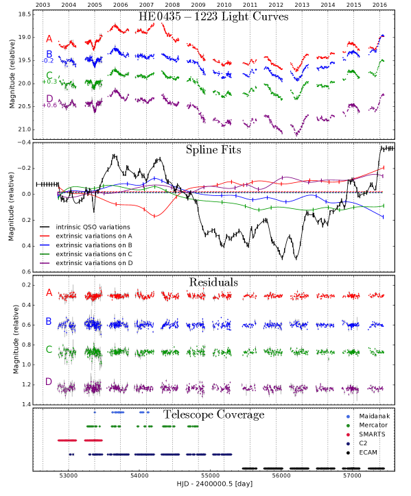
Following the encouraging results obtained at NOT, ESO and Wise, long-term monitoring campaigns were organized to measure time delays in a systematic way. Two main teams invested effort in this research: the OSU group lead by C.S. Kochanek (OSU, USA) and the COSMOGRAIL (COSmological MOnitoring of GRAvItational Lenses) program led by F. Courbin and G. Meylan at EPFL, Switzerland (e.g. Courbin et al, 2005; Eigenbrod et al, 2005). Both monitoring programs involve 1-m class telescopes with a temporal sampling of 2 to 3 observing epochs per week and a signal-to-noise of typically 100 per quasar image and per epoch. Both projects started in 2004 and are so far the main (but not only) source of time-delay measurements. Early results from the OSU program were obtained in 2006 for HE 04351223 (Kochanek et al, 2006) while COSMOGRAIL delivered its first results starting in 2007 for SDSS J1650+4251 (Vuissoz et al, 2007), WFI J20334723 (Vuissoz et al, 2008) and HE 04351223 (Courbin et al, 2011a). More recent time-delay measurements from COSMOGRAIL were obtained for RX J11311231 (Tewes et al, 2013b), HE 04351223 (Bonvin et al, 2017) as well as SDSS J1206+4332 and HS 2209+1914 (Eulaers et al, 2013) and SDSS J1001+5027 (Rathna Kumar et al, 2013). An example of COSMOGRAIL light curve is given in Fig. 1. These data are analysed jointly with the H0LiCOW program (see Section 1.4).
Other recent studies for specific objects include Giannini et al (2017) for WFI 20334723 and HE 00471756, and Shalyapin and Goicoechea (2017) reporting a delay for SDSS J1515+1511. Hainline et al (2013) measure a tentative time delay for SBS 0909+532, although the curves suffer from strong microlensing. Finally, two (long) time delays have been estimated for two quasars lensed by a galaxy group/cluster: SDSS J1029+2623 (Fohlmeister et al, 2013) and SDSSJ1004+4112 (Fohlmeister et al, 2008). These may not be ideal for cosmological applications though, as a complex lens model for a cluster is harder to constrain than models at galaxy-scale, unless the cluster has additional constraints coming from multiple background sources at different redshifts being strongly lensed.
With the observing cadence of 1 point every 3-4 nights and an SNR of 100 per epoch, the current data can catch quasar variations of the order of 0.1 mag in amplitude, arising on time-scales of months. These time scales are unfortunately of the same order of magnitude as the microlensing variations (see 2nd panel of Fig. 1) making it hard to disentangle between intrinsic and extrinsic variations. For this reason, lensed quasars must be monitored for extended periods of time, typically a decade, to infer any reliable time-delay measurement.
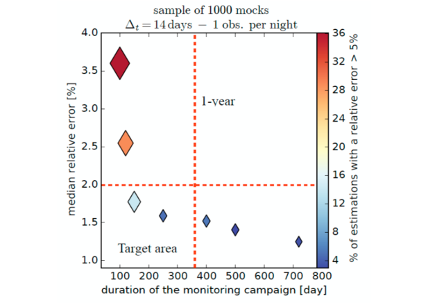
Going beyond current monitoring campaigns like COSMOGRAIL and others is possible, but measuring massively time delays for dozens of lensed quasars requires a new observing strategy to minimize the effect of microlensing and to measure time delays in individual objects in less than 10 years! One solution is to observe at high cadence (1 day-1) and high SNR, of the order of 1000. In this way, very small quasar variations can be caught, on time scales much shorter than microlensing hence allowing the separation of the two signals in frequency. We show with 1000 mock light curves that mimic those of HE 04251223 (Fig. 1) that time delays can be measured precisely in only 1 observing season. In doing the simulation, we include realistic microlensing and fast quasar variations with a few mmag amplitude. We then run PyCS, the COSMOGRAIL curve-shifting algorithm (Tewes et al, 2013a; Bonvin et al, 2016), to recover the fiducial time delay of 14 days. Fig. 2 summarizes our results and provides the length of the monitoring campaign needed to reach a desired relative precision on the time delay, assuming daily observations and an SNR of 1000 per epoch. It appears that a typical 2% precision is achievable in 1 observing season with a 10% failure rate. Doing two seasons allows one to reach the percent precision and a failure rate below 3%. At the time this paper is being written, an intensive lens monitoring program has been started at the 2.2m MPI telescope at La Silla Observatory, with the above characteristics. Three targets have been observed for 1 semester and time delays have been measured to a few percents for all three! The first of these is presented in Courbin et al (2017) and features a 1.8% measurement of one of the delays in the newly discovered quadruple lens DES J04085354 (Lin et al, 2017; Agnello et al, 2017).
Finally, we note that although quasars have been used so far to implement the time delay method, the original idea of Refsdal was to use lensed supernovae. The first systems have finally be found, as mentioned in Section 1.2: SN Refsdal (e.g. Kelly et al, 2015, 2016a; Rodney et al, 2016) and iPTF16geu (e.g. Goobar, 2017; More et al, 2017). With the advent of large imaging surveys such as the Zwicky Transient Facility and the Large Synoptic Survey Telescope, prospects to find lensed supernovae are excellent (e.g. Goldstein and Nugent, 2017). As supernovae have known light curves, one can measure the time delay by fitting a template to the observed light curves in the lensed images, hence giving much more constraining power than quasars whose photometric variations are close to a random walk. In addition, if the lensed supernova is a Type Ia, then two cosmological probes are available in the same object, hence provide a fantastic cross-check of otherwise completely different methods: standard candles and a geometrical method, provided microlensing effects could be corrected (Dobler and Keeton, 2006; Yahalomi et al, 2017; Goldstein et al, 2018).
For all the above reasons, we believe that the future of time-delay cosmography resides in lensed supernovae and in high-cadence monitoring of lensed quasars. However, Tie and Kochanek (2018) recently pointed out that microlensing by stars in the lensing galaxy can introduce a bias in the time-delay measurements. This is due to a combination of differential magnification of different parts of the source and the source geometry itself. The net result is that cosmological time delays can be affected both in a statistical and a systematic way by microlensing. The effect is absolute, with biases on time delays of the order of a day for lensed quasars and tenths of a day for lensed supernovae. Mitigation strategies have been successfully devised (Chen et al, 2018) for lensed quasars and the effect seems less pronounced in lensed supernovae than in lensed quasars (Goldstein et al, 2018; Foxley-Marrable et al, 2018; Bonvin et al, 2018), but clearly this new effect must be accounted for in any future work in the field.
Lens mass modeling
To convert the time delays into a measurement of the time-delay distance via equation (1), one needs to determine the Fermat potential , which depends both on the mass distribution of the main strong-lens galaxy and the mass distribution of other galaxies along the line of sight.
The mass distribution of the main strong-lens galaxy can be modeled using either simply parametrized profiles (e.g., Kormann et al, 1994; Barkana, 1998; Golse and Kneib, 2002) or grid-based approaches (e.g., Williams and Saha, 2000; Blandford et al, 2001; Suyu et al, 2009; Vegetti and Koopmans, 2009). The total mass distribution of galaxies appear to be well described by profiles close to isothermal (e.g., Koopmans et al, 2006; Barnabè et al, 2011; Cappellari et al, 2015), even though neither the baryons nor the dark matter distribution follow isothermal profiles. Even in the complex case of the gravitational lens B1608+656 with two interacting lens galaxies, simply parametrized profiles provide a remarkably good description of the galaxies when compared to the pixelated lens potential reconstruction (Suyu et al, 2009). Therefore, most of the current mass modeling for time-delay cosmography use simply parametrized profiles, either for the total mass distribution (e.g., Koopmans et al, 2003; Fadely et al, 2010; Suyu et al, 2010, 2013; Birrer et al, 2015b) or for separate components of baryons and dark matter (e.g., Courbin et al, 2011b; Schneider and Sluse, 2013; Suyu et al, 2014; Wong et al, 2017).
The source (quasar) properties need to be modeled simultaneously with the lens mass distribution to predict the observables. In particular, source position and intensity are needed to predict the positions, fluxes and time delays of the lensed quasar images, whereas the source surface brightness distribution (of the quasar host galaxy) is needed to predict the lensed arcs. These observables (image positions, fluxes and delays of the multiple quasar images, and lensed arcs) are then used to constrain the parameters of the lens mass model and the source. Several softwares are available publicly for modeling lens systems, including Gravlens (Keeton, 2001), lenstool (Jullo et al, 2007), glafic (Oguri, 2010) and Lensview (Wayth and Webster, 2006).
Observed quasar image positions, fluxes and delays provide around a dozen of constraints for quads (four-image systems) and even fewer constraints for doubles (two-image systems). Thus lens mass models using only these quasar observables are often not precisely constrained. In particular, the radial profile slope of the lens galaxy is strongly degenerate with (e.g., Wucknitz, 2002; Suyu, 2012). The time delays depend primarily on the average surface mass density between the multiple images, and thus provide information on the radial profile slope (Kochanek, 2002). Nevertheless, even with multiple time delays from quad systems, it is difficult to infer the slope precisely to better than precision333 in terms of impact on . While mass distribution of massive early-type galaxies, which are the majority of lens galaxies, are close to being isothermal, there is an intrinsic scatter in the slope of about (Koopmans et al, 2006; Barnabè et al, 2011). For precise and accurate measurement of a lens system, it is important to measure directly, at the few percent level, the radial profile slope of the lens galaxy near the lensed images of the quasars. This requires more observations of the lens system, beyond just the multiple point images of lensed quasars.
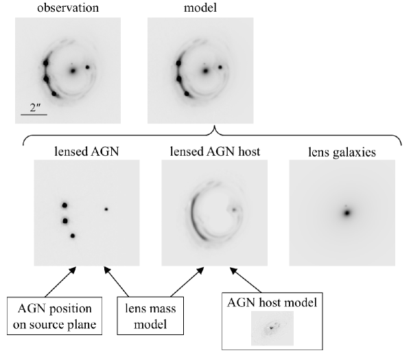
Over the past decade, multiple methods have been developed to make use of the lensed arcs (lensed host galaxies of the quasars) to constrain the lens mass distribution. The source intensity distribution can be described by simply parametrized profiles, such as Gaussians or Sersic (e.g., Brewer and Lewis, 2008; Oguri, 2010; Marshall et al, 2007; Oldham et al, 2017), or on a grid of pixels, either regular (e.g., Wallington et al, 1996; Warren and Dye, 2003; Koopmans, 2005; Suyu et al, 2006) or adaptive (e.g., Dye and Warren, 2005; Vegetti and Koopmans, 2009; Tagore and Keeton, 2014; Nightingale and Dye, 2015), or based on basis functions (e.g., Birrer et al, 2015a, Joseph et al. in prep.). These lensed arcs, when imaged with HST or ground-based telescopes assisted with adaptive optics, contain thousands of intensity pixels and thus allow the measurement of the radial profile slope of the lens galaxies with a precision of a few percent (e.g., Dye and Warren, 2005; Suyu, 2012; Chen et al, 2016), that are required for cosmography. In Fig. 3, we show an example of the mass modeling using the full surface brightness distributions of quasar host galaxy.
Once a model of the surface mass density is obtained, lens theory states that the following family of models fits equally well to the observed lensing data:
| (7) |
where is a constant. This transformation is analogous to adding a constant mass sheet in convergence, and rescaling the mass distribution of the strong lens (to keep the same mass within the Einstein radius); it is therefore called the “mass-sheet degeneracy” (Falco et al, 1985; Schneider and Sluse, 2013, 2014; Schneider, 2014). Such a transformation corresponds to a rescaling of the background source coordinate by a factor , leaving the observed image morphology and brightness invariant. Furthermore, the Fermat potential transforms as
| (8) |
Therefore, for given observed time delays , equations (6) and (8) imply that the time-delay distance would be scaled by . The mass-sheet degeneracy has thus a direct impact on cosmography in measuring .
While so far is simply a constant in this mathematical transformation (equation 7), we can identify it with the physical external convergence, , due to mass structures along the sight line to the lens system. By gathering additional data sets beyond that of the strong lens system, we can infer and thus measure . Two practical ways to break the mass-sheet degeneracy are (1) studies of the lens environment, to estimate based on the density of galaxies in the strong-lens line of sight in comparison to random lines of sight (e.g., Momcheva et al, 2006; Fassnacht et al, 2006; Hilbert et al, 2007; Suyu et al, 2010; Greene et al, 2013; Collett et al, 2013; Rusu et al, 2017; Sluse et al, 2017; McCully et al, 2017), and (2) stellar kinematics of the strong lens galaxy, which provides an independent mass measurement within the effective radius to complement the lensing mass enclosed within the Einstein radius (e.g., Grogin and Narayan, 1996; Koopmans and Treu, 2002; Barnabè et al, 2009; Suyu et al, 2014). The time-delay distance can then be inferred via
| (9) |
where is the modeled time-delay distance without accounting for the presence of . In practice, both lens environment characterisations and stellar kinematics are employed to infer for cosmography (e.g., Suyu et al, 2010, 2013; Birrer et al, 2015b; Wong et al, 2017). The stellar kinematic data further help constrain the strong-lens mass profile (e.g., Suyu et al, 2014).
Lens systems that have massive galaxies close in projection (within ) to the strong lens, but at a different redshift from the strong lens, will need to be accounted for explicitly in the strong lens model. In such cases, multi-lens plane modeling is needed (e.g., Blandford and Narayan, 1986; Schneider et al, 1992; Gavazzi et al, 2008; Wong et al, 2017, Suyu et al., in preparation), but equation (1) for single-lens plane is then not directly valid. In particular, there is not a single time-delay distance, but rather there are multiple combination of distances between the multiple planes. Nonetheless, for some cases, one could obtain an effective time-delay distance as if it were a single-lens plane system (see, e.g., Wong et al, 2017, for details).
As noted in Section 1.1, with stellar kinematic and time-delay data, we can infer the angular diameter distance to the lens, , in addition to (Paraficz and Hjorth, 2009; Jee et al, 2015; Birrer et al, 2015b; Shajib et al, 2017). Measurement of is often more sensitive to the dark energy parameters (for typical lens redshifts , see e.g., Fig. 2 of Jee et al, 2016), and can also be used as an inverse distance ladder to infer (Jee et al., submitted). Currently, the precision in is limited by the uncertainty in the single-aperture averaged velocity dispersion measurement and the unknown anisotropy of stellar orbits (Jee et al, 2015). Nonetheless, we anticipate that spatially resolved kinematic data will help to constrain more precisely .
We have focussed here on the advances in getting and from individual lenses with exquisite follow-up data to control the systematic uncertainties. Alternatively, one could analyse a sample of lenses and constrain a global parameter that is common to all the lenses (e.g., Saha et al, 2006; Oguri, 2007; Sereno and Paraficz, 2014), assuming that the systematic effects for the lenses average out. For small samples, this assumption might not be valid. Nonetheless, in the future where thousands of lensed quasars are expected (Oguri and Marshall, 2010) but most of which will not have exquisite follow-up observations, this large sample of lenses could provide information on the population of lens galaxies as a whole for cosmography (P. J. Marshall & A. Sonnenfeld, priv. comm.). We therefore advocate getting exquisite follow-up observations of a sample of lenses to reach an measurement with 1% uncertainty (Jee et al, 2016; Shajib et al, 2017), with the other lenses providing information on the profiles of galaxies to use in the mass modeling.
1.4 Distance measurements and cosmological inference
There are so far only a few lensed quasars for which all required data exist to do time-delay cosmography, i.e., with time-delay measurements to a few percent, deep HST images showing the lensed image of the host galaxy, deep spectra of the lens to measure the velocity dispersion, and multiband data to map the line of sight contribution to the lensing potential.
Some of the best time-delay measurements available to date include the radio time delay for B1608+656 (Fassnacht et al, 1999, 2002) and the two optical measurements of COSMOGRAIL for RX J11311231 (Tewes et al, 2013b), and HE 04351223 (Bonvin et al, 2017). These 3 quadruply imaged quasars, for which all the ancillary imaging and spectroscopic data are also available, gave birth to the H0LiCOW program (Suyu et al, 2017), which capitalizes on more than a decade of COSMOGRAIL monitoring as its name reflects: H0 Lenses in COMOGRAIL’s Wellspring. With the precise time-delay measurements of COSMOGRAIL, H0LiCOW addresses what has been so far limiting the effectiveness of strong lensing in delivering reliable measurements: the different systematics at work at each step leading to a value for the Hubble constant.
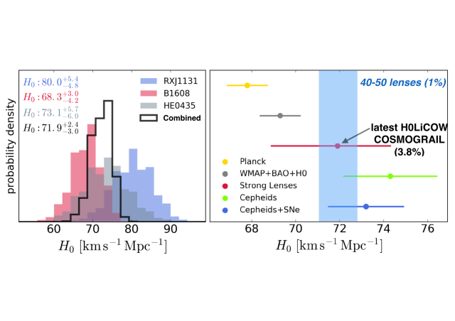
The most recent work by H0LiCOW is summarized in the left panel of Fig. 4 (Bonvin et al, 2017), based on state-of-the-art lens mass modeling and characterisations of mass structures along the line of sight (Sluse et al, 2017; Rusu et al, 2017; Wong et al, 2017; Tihhonova et al, 2017). In the right panel of Fig. 4, we compare the value of from H0LiCOW with other fully independent cosmological probes such as Type Ia supernovae, Cepheids, and CMB(+BAO) for a CDM cosmology. With the current error bars claimed by each probe there exist a tension between local measurements of (e.g., Freedman et al, 2012; Efstathiou, 2014; Riess et al, 2018) and the value by the Planck team. When completed, H0LiCOW will feature 5 lenses, with an accuracy on of the order of 3% (Suyu et al, 2017), but reaching close to 1% precision is possible. This will be enabled by working on several fronts simultaneously, by finding more lenses, measuring up to 50 new time delays, and refining the lens modeling tools to mitigate degeneracies between model parameters. Chapter 8 on “Towards a self-consistent astronomical distance scale” provides more details about the (expected) future of quasar time delay cosmography.
2 Baryon Acoustic Oscillations
2.1 BAO as a standard ruler
The universe has been expanding, and thus the universe in the earlier stage was much smaller, denser and hotter than today. In such an early universe, electrons interacted with photons via Compton scattering and with protons via Coulomb scattering. Thus, the three components acted as a mixed fluid (Peebles and Yu, 1970). They were in the equilibrium state due to the gravity of protons and pressure of photons, and oscillated as sound modes. These oscillations are called baryon acoustic oscillations (BAO) (see Bassett and Hlozek (2010) and Weinberg et al (2013) for a comprehensive review). It moved with the speed of sound , where the ratio of photon density () to baryon density () is defined as .
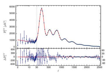
At recombination (), photons decouple from the baryons and start to free stream. We observe the photons as a map of cosmic microwave background (CMB). The left panel of Fig. 5 shows the angular power spectrum of the latest data of the CMB anisotropy probe, Planck satellite (Planck Collaboration et al, 2016a). One can see a clear oscillation feature in the power spectrum, which is characterized by the sound horizon scale at recombination, expressed as (Hu and Sugiyama, 1996; Eisenstein and Hu, 1998)
| (10) |
where is the redshift at recombination. is the Hubble parameter,
| (11) |
where (previously introduced in Section 1.1), and are the matter, radiation and dark energy density parameters, respectively, and is the equation-of-state parameter of dark energy and the simplest candidate for dark energy, the cosmological constant , gives . With standard cosmological models, Mpc. From the Planck observation, it is constrained to Mpc.
2.2 Probing BAO in galaxy distribution
After the recombination, motion of the baryons becomes non-relativistic. The perturbation of baryons then starts to grow at their locations and interact with the perturbation of dark matter. Thus the baryon acoustic feature should be imprinted onto the late-time large-scale structure of the Universe. Theoretically it is predicted to produce the overdensity at the sound horizon scale, Mpc. It is, however, observationally not easy because the observation of BAO signal requires the number of tracers of matter overdensity field to be large enough at the scale to overcome the cosmic variance.
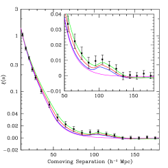
In 2005, detection of the BAO was reported almost simultaneously by two independent groups using the Sloan Digital Sky Survey (SDSS) (Eisenstein et al, 2005) and the 2dF Galaxy Redshift Survey (2dFGRS) (Cole et al, 2005). The right panel of Fig. 5 shows the two-point correlation function obtained from the SDSS galaxy sample by Eisenstein et al (2005). The 2-point correlation function is defined as an excess of the probability that one can find pairs of galaxies at a given scale from the case of a random distribution. Thus the scales where and correspond to the statistically overdense and underdense regions respectively. The bump seen around ( Mpc) is the feature of BAO, and the scale of the bump corresponds to the sound horizon scale at recombination. The inset of the right panel of Fig. 5 zooms into the feature. Unlike observations of the CMB, galaxy redshift surveys are the observation of 3 dimensional space. The peak scale of BAO should be isotropic because the scale corresponds to the sound horizon at recombination. On the other hand, the BAO scale along the line of sight depends on while the BAO scale perpendicular to the line of sight depends on the comoving angular diameter distance , where is expressed in flat universe as equation (3) with , or,
| (12) |
Thus, the scale of BAO probed by a galaxy correlation function has a cosmology dependence of
| (13) |
The BAO scale probed by the CMB anisotropy at high redshift and the galaxy distribution at low redshift should be the same. Moreover, the power spectrum with the acoustic features has been precisely determined for the CMB and interpreted using linear cosmological perturbation theory (see the left panel of Fig. 5). Thus the detection of BAO in the galaxy distribution enables us to constrain , and hence the geometric quantities such as , , and in equation (11) (Eisenstein et al, 2005).
2.3 Anisotropy of BAO and Alcock-Paczynski
The method presented above does not use all of the information encoded in BAO. To maximally extract the cosmological information, we need to measure the correlation function as functions of separations of galaxy pairs perpendicular () and parallel () to the line of sight, , where . In this way, in principle we can constrain and using the transverse and radial BAO measurements, respectively. Given the cosmological dependence of angular and radial distances (equations 11 and 12), the shape of the BAO peak is distorted if the wrong cosmology is assumed. This effect was first pointed out by Alcock and Paczynski (1979, AP).
In fact, the AP test using the anisotropy of BAO has additional advantages. Since the BAO scale should correspond to the sound horizon at recombination, it should be a constant. Thus, we can determine the geometric quantities by requiring that the radial BAO scale equals to the angular BAO scale. We no longer need to know the exact value of nor need to rely on the CMB experiment (see e.g., Seo and Eisenstein, 2003; Matsubara, 2004). This is particularly important in the context of measuring given the tension in between the local measurements and the inference by the Planck team in flat CDM (see Section 1.4).
In galaxy surveys, the distance to each galaxy is measured through redshift, thus it gives the sum of the true distance and the contribution from the peculiar motion of the galaxies and it produces an anisotropy in galaxy distribution along the line of sight, which are called redshift-space distortions (RSD). Since the velocity field of a galaxy is caused by gravity, the anisotropy contains additional cosmological information. This effect is called the Kaiser effect, named after Kaiser (1987) who proposed RSD as a cosmological probe in the linear perturbation theory limit. Since the velocity field is related to the density field through the continuity equation, the anisotropy constrains the quantity , defined as the logarithmic derivative of the density perturbation, . See Okumura et al (2016) for the constraint on from RSD as a function of including the high- measurement.
By simultaneously measuring the BAO and RSD and combining them with the CMB anisotropy power spectrum, we can obtain a further constraint on additional geometric quantities, such as the time evolution of , the neutrino mass , etc. The cosmological results, presented below, correspond to this case.
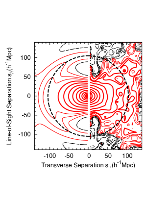
The correlation function in 2D space including the BAO scales has been measured by Okumura et al (2008) for the first time using the same galaxy sample as Eisenstein et al (2005). The right-hand side of the left panel in Fig. 6 shows the measured correlation function, while the left-hand side shows the best fitting model based on linear perturbation theory (Matsubara, 2004). The circle shown at the scale again corresponds to the sound horizon at recombination. The distorted, anisotropic contours shown at the smaller scales are the RSD effect caused by the velocity field.
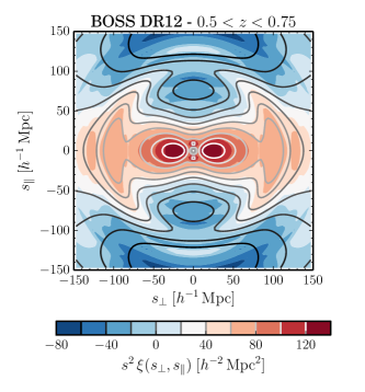
The right panel of Fig. 6 is the latest measurement of the correlation function using the SDSS-III Baryon Oscillation Spectroscopic Survey (BOSS) DR12 sample (Alam et al, 2016). The anisotropic feature of BAO is more clearly detected due to the improvement of the data, both in the number of galaxies and the survey volume: the data of the DR12 sample used in Alam et al (2016) comprised 1.2 million galaxies over the volume of , whose numbers are respectively 25 times and 9 times larger than those of the DR3 sample used in Okumura et al (2008).
2.4 Constraints on BAO distance scales and
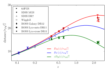
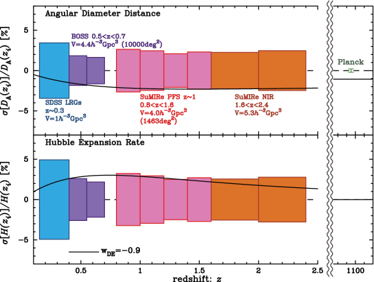
The left panel of Fig. 7 shows the summary of the three distance measures obtained by BAO in various galaxy surveys (Aubourg et al, 2015). The -axis is the ratio of each distance and , divided by . The blue points are the measurement of from the angularly-averaged BAO, while the red and green points are respectively the measurements of and obtained from the anisotropy of BAO, where is the radial distance defined as . The three lines with the same color as the points are the corresponding predictions of the CDM model obtained by Planck (Planck Collaboration et al, 2016a). Nice agreement between BAO measurements from galaxy surveys and Planck cosmology can be seen. However, the agreement with the WMAP cosmology is equivalently good in terms of distance measures (Anderson et al, 2014).
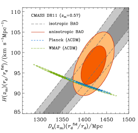
The right panel of Fig. 7 focuses on currently the largest survey, the BOSS survey at (Anderson et al, 2014). Here the joint constraints on and are shown. The gray contours are obtained from the 1D BAO analysis (see section 2.2). Because the 1D BAO constrains , there is a perfect degeneracy between and . On the other hand, the solid orange contours are from the 2D BAO analysis where the degeneracy is broken to some extent (Section 2.3). The obtained constraints on the distance scales are as tight as the flat CDM constraints from the CMB experiments, Planck (dashed blue) and WMAP (dot-dashed green). Future galaxy surveys will enable us to measure BAO more accurately and determine the cosmic distance scales with higher precision (see Section 2.5).
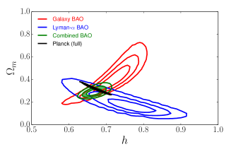
Let us move onto the constraints on cosmological models using BAO observations. The left panel of Fig. 8 shows the joint constraints on the matter density parameter and the Hubble constant obtained from the measurements of BAO anisotropy (Aubourg et al, 2015). The red and blue contours are the constraints from the BAO measured from the various galaxy samples at and from the Ly forest at , respectively, as shown in the left panel of Fig. 7. Since these constraints are not very tight, the constrained from either galaxy BAO or Ly BAO is consistent with other probes including the local measurements. The combination of these two BAO probes largely tightens the constraint on and causes a slight, tension as we will see below. With being marginalized over, the Hubble constant is constrained to ( C. L.) (Aubourg et al, 2015).
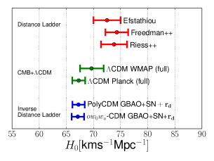
The right panel of Fig. 8 summarizes the comparison of constraints from the BAO measurement and other probes. Augmenting Fig. 4, the top three points are obtained from the distance ladder analysis, showing constraints from the local universe from three independent teams (Riess et al, 2016a; Freedman et al, 2012; Efstathiou, 2014). The green, two middle points are the constraints from the two CMB satellite probes, WMAP and Planck. The bottom two points are from the inverse distance ladder analysis, namely the combination of BAO and SN distance measures. As seen from the figure, those from the Planck and the inverse ladder measurements have a mild but non-negligible tension with the distance-ladder measurements, about . The discrepancy could be due to just systematics, or a hint of new physics. We will need further observational constraints to resolve these discrepancies.
2.5 Future BAO Surveys
BAO are considered as a probe least affected by systematic biases to measure distance scales, even beyond the local universe (), and thus are a promising tool to reveal the expansion history of the universe and constrain the cosmological model. To improve the precision of the distance measurement, a dominant source of error on BAO observations is the cosmic variance. There are larger, ongoing and planned galaxy redshift surveys, such as extended BOSS (eBOSS) (Dawson et al, 2016), Subaru Prime Focus Spectrograph (PFS) (Takada et al, 2014), and Dark Energy Spectroscopic Instrument (DESI) (DESI Collaboration et al, 2016). With the larger survey volumes, these surveys will measure distance scales using BAO with percent-level precisions. These surveys are also deep and can reveal fainter sources, and hence enable us to extend the distance scales to more distant parts of the universe.
As an example, Fig. 9 presents the accuracies of constraining the angular diameter distance and Hubble expansion rate expected from the analysis of anisotropic BAO (see Section 2.3) of the PFS survey at the Subaru Telescope. The PFS will observe the universe at by using [OII] emitters as a tracer of the large-scale structure. The survey volume of each redshift slice is on the order of and the number density is larger than , which are comparable to the existing SDSS and BOSS surveys at . Hence, one will be able to achieve a few percent constraints on and at high redshifts, almost the same as those obtained from the low- surveys. Deep galaxy surveys such as the PFS allow for constraining not only the expansion history of the universe but also dark energy (see the solid line of Fig. 9).
3 Intensity Mapping
3.1 21cm Intensity Mapping BAO
As we described in Section 2, current BAO measurements are enabled by large galaxy spectroscopic surveys, and the resulting constraining power on cosmological parameters generally scales as the effective survey comoving volume. Specifically, the precision of cosmological parameter constraints scales as , where is the number of modes, or in the case of 3D map where is the comoving volume and the maximum useful comoving wavenumber. This scale is often given by the non-linearity scale, , where the complexity of baryonic astrophysics on galaxy and galaxy-cluster scales limits our ability to extract cosmological parameters. Improving parametric precision will therefore require larger volumes, which requires mapping higher redshift volumes that have the added benefit of increasing . The emerging technique of 21 cm Intensity Mapping appears to be a very promising way to reach this goal.
Galaxy redshifts can be measured at radio wavelengths using the 21 cm hyperfine emission of atomic neutral hydrogen (HI). The 21 cm line is unique in cosmology because for cm it is the dominant astronomical line emission, i.e., for all positive redshifts and all cosmological emission. So to a good approximation the wavelength of a spectral feature can be converted to a Doppler redshift without the uncertainty and ambiguity of having to first identify the atomic transition. The direct determination of redshifts using 21 cm data can be compared to the corresponding optical technique, which requires identifying a suitable subset of target galaxies (photometry), then obtaining an optical spectrum, and finally finding some unique combination of emission and absorption lines that allow an unambiguous determination of the redshift for that galaxy (spectroscopy).
The 21 cm signal has been used to conduct galaxy redshift surveys in the local Universe around (Martin et al, 2010; Zwaan et al, 2001) and out to (Fernández et al, 2016). Beyond this redshift, current radio telescopes do not have sufficient collecting area or sensitivity to make 21 cm surveys using individual galaxies.
A radically different technique, HI intensity mapping (HIM), has been proposed (Chang et al, 2008; Wyithe et al, 2008). It uses maps of 21 cm emission where individual galaxies are not resolved. Instead, it detects the combined emission from the many galaxies that occupy large () voxels. The technique allows 100 m class telescopes such as the Green Bank Telescope (GBT), which only have angular resolution of several arc-minutes, to rapidly survey enormous comoving volumes at (Abdalla and Rawlings, 2005; Peterson et al, 2006; Wyithe et al, 2007; Chang et al, 2008; Wyithe et al, 2008; Tegmark and Zaldarriaga, 2009, 2010; Seo et al, 2010). A number of authors (Seo et al, 2010; Xu et al, 2015; Bull et al, 2015) have studied the overall promise of the intensity mapping technique. Chang et al (2010); Masui et al (2013) and Switzer et al (2013) have reported the first detections in cross-correlations and upper limits to the 21cm auto-power spectrum using the Green Bank Telescope (GBT).
Challenges
One of the major challenges for 21 cm intensity mapping is the mitigation of radio foregrounds, which are predominantly Galatic and extragalactic synchrotron emissions, and are at least times brighter in intensity than the 21 cm emission. The two can be distinguished because the former have smooth spectra and the latter trace the underlying large-scale structure and have spectral structures. The brightness temperature of the synchrotron foreground typically has a spectral dependence of , or , and is thus more severe at higher redshifts. Note it has not yet been demonstrated whether the synchrotron radiation is indeed spectrally smooth down to one part of or higher and therefore can in principle be suppressed by this factor to reveal the 21cm fluctuation signals. However, since the BAO wiggles have very specific structures, we can potentially select Fourier modes that are observationally accessible in scale and redshifts (Chang et al, 2008; Seo et al, 2010).
The 21 cm features we are most interested in are the relatively non-smooth BAO ‘wiggles’. Unfortunately radio telescopes are diffraction-limited and the beam patterns depend on frequency, which mixes angular and frequency dependence. Since the foregrounds are not smooth in position across the sky it is a nontrivial task to identify and subtract the smooth frequency foregrounds with sufficient accuracy so as to reveal the 21 cm emission. It is easier if we go to very small radial scales, but to get the most cosmological information out of the data we would need to remove the foregrounds over the largest range of scales possible. Shaw et al (2013, 2015) have demonstrated that this is achievable in principle.
To achieve the foreground subtraction goal and to make accurate 3D maps we need a very accurate model of the beam patterns and characterization of the mapping between the observed and true skies. Liao et al (2016) have recently demonstrated accurate measurements of the polarized GBT beam to sub-percent level, which is critical for polarized foreground mitigation. Developing and demonstrating the efficacy of methods to model and calibrate large dataset is also necessary to achieve the main objective.
Future Prospects
As discussed in Section 2, baryon acoustic oscillations provide a convenient standard ruler in the cosmological large scale structure (LSS) allowing a precise measurement of the distance-redshift relation over cosmic time. This distance redshift relation is measured, whether by BAO, SNe-Ia surveys, or weak lensing, to characterize the dark energy; it is augmented by the growth rate of inhomogeneities as well as redshift-space distortions. All three of these quantities can be measured in HI surveys even though to-date, only optical instruments have detected BAO features in the power spectrum.
Going forward requires the most cost-effective way to map the largest cosmological volume, and this may be radio spectroscopy through intensity mapping. One unique advantage of 21cm Intensity Mapping is the fact that the 21 cm signal is in principle observable from up to a redshift of , when its spin temperature decouples from the Cosmic Microwave Background radiation. The vast majority of the cosmic volume is only visible during the dark ages via the 21 cm radiation from neutral hydrogen, before the onset of galaxy formation. 21 cm Intensity Mapping thus provides a unique access to measuring LSS during this period (Tegmark and Zaldarriaga, 2009, 2010). Besides, 21 cm intensity mapping has a set of observational systematics that should be largely uncorrelated with the systematic effects in optical surveys.
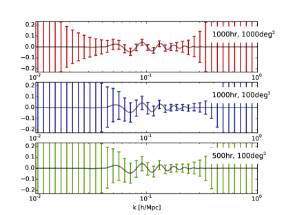
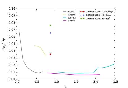
The on-going low-z GBT-HIM survey is a step along the way to a dark ages radio survey. We have made BAO forecasts based on the expected performance of the array. We assume the seven-beam array has a 700-850 MHz frequency coverage with a total system temperature of 33K. The BAO forecasts are consistent with predictions in Masui et al (2010) and are in reasonable agreement with those of Bull et al (2015). We consider three scenarios with different observing depth and sky coverage: 500 or 1000 hours of on-sky GBT observations, covering 100 or 1000 deg2 of sky areas. The expected errors on the BAO wiggles and the fractional distance constraints are shown in Fig. 10. We anticipate to yield a 3.5% error on the BAO distance at with 1000 hours of GBT observing time. The bottom panel of Fig. 10 also shows recent constraints from WiggleZ (Drinkwater et al, 2010) and the BOSS surveys (Anderson et al, 2014) at lower redshifts, and forecasts for CHIME (Bandura et al, 2014) and WFIRST (Spergel et al, 2015). With the demonstrated results and good understanding of systematic effects at the GBT, and with very different astrophysical and measurement systematics from optical/IR spectroscopic redshift surveys, we anticipate the GBT-HIM array can make a firm detection of the BAO signature at z0.8 with the HI intensity mapping technique, and contribute to the future of large-scale structure surveys and the field of 21-cm cosmology. Other on-going experiments such as CHIME (Bandura et al, 2014) and HIRAX (Newburgh et al, 2016) will reach and probe even larger cosmological volume.
Acknowledgements.
Open access funding provided by the Max Planck Society. We thank ISSI-BJ for the kind hospitality and an engaging workshop. We would like to acknowledge Vivien Bonvin for providing some of the figures in this review. T.O. thanks Anze Slosar, Shun Saito and Atsushi Taruya for useful discussions on interpretations of cosmological constraints from the BOSS survey. S.H.S. thanks the Max Planck Society for support through the Max Planck Research Group. F.C. acknowledges support from the Swiss National Science Foundation (SNSF). T.O. acknowledges support from the Ministry of Science and Technology of Taiwan under the grant MOST 106-2119-M-001-031-MY3.References
- Abdalla and Rawlings (2005) Abdalla FB, Rawlings S (2005) Probing dark energy with baryonic oscillations and future radio surveys of neutral hydrogen. MNRAS 360:27–40, DOI 10.1111/j.1365-2966.2005.08650.x, arXiv:astro-ph/0411342
- Agnello et al (2017) Agnello A, Lin H, Buckley-Geer L, Treu T, Bonvin V, Courbin F, Lemon C, Morishita T, Amara A, Auger MW, Birrer S, Chan J, Collett T, More A, Fassnacht CD, Frieman J, Marshall PJ, McMahon RG, Meylan G, Suyu SH, Castander F, Finley D, Howell A, Kochanek C, Makler M, Martini P, Morgan N, Nord B, Ostrovski F, Schechter P, Tucker D, Wechsler R, Abbott TMC, Abdalla FB, Allam S, Benoit-Lévy A, Bertin E, Brooks D, Burke DL, Rosell AC, Kind MC, Carretero J, Crocce M, Cunha CE, D’Andrea CB, da Costa LN, Desai S, Dietrich JP, Eifler TF, Flaugher B, Fosalba P, García-Bellido J, Gaztanaga E, Gill MS, Goldstein DA, Gruen D, Gruendl RA, Gschwend J, Gutierrez G, Honscheid K, James DJ, Kuehn K, Kuropatkin N, Li TS, Lima M, Maia MAG, March M, Marshall JL, Melchior P, Menanteau F, Miquel R, Ogando RLC, Plazas AA, Romer AK, Sanchez E, Schindler R, Schubnell M, Sevilla-Noarbe I, Smith M, Smith RC, Sobreira F, Suchyta E, Swanson MEC, Tarle G, Thomas D, Walker AR (2017) Models of the strongly lensed quasar DES J0408-5354. MNRAS472:4038–4050, DOI 10.1093/mnras/stx2242, 1702.00406
- Alam et al (2016) Alam S, Ata M, Bailey S, Beutler F, Bizyaev D, Blazek JA, Bolton AS, Brownstein JR, Burden A, Chuang CH, Comparat J, Cuesta AJ, Dawson KS, Eisenstein DJ, Escoffier S, Gil-Marín H, Grieb JN, Hand N, Ho S, Kinemuchi K, Kirkby D, Kitaura F, Malanushenko E, Malanushenko V, Maraston C, McBride CK, Nichol RC, Olmstead MD, Oravetz D, Padmanabhan N, Palanque-Delabrouille N, Pan K, Pellejero-Ibanez M, Percival WJ, Petitjean P, Prada F, Price-Whelan AM, Reid BA, Rodríguez-Torres SA, Roe NA, Ross AJ, Ross NP, Rossi G, Rubiño-Martín JA, Sánchez AG, Saito S, Salazar-Albornoz S, Samushia L, Satpathy S, Scóccola CG, Schlegel DJ, Schneider DP, Seo HJ, Simmons A, Slosar A, Strauss MA, Swanson MEC, Thomas D, Tinker JL, Tojeiro R, Vargas Magaña M, Vazquez JA, Verde L, Wake DA, Wang Y, Weinberg DH, White M, Wood-Vasey WM, Yèche C, Zehavi I, Zhai Z, Zhao GB (2016) The clustering of galaxies in the completed SDSS-III Baryon Oscillation Spectroscopic Survey: cosmological analysis of the DR12 galaxy sample. ArXiv e-prints 1607.03155
- Alcock and Paczynski (1979) Alcock C, Paczynski B (1979) An evolution free test for non-zero cosmological constant. Nature281:358, DOI 10.1038/281358a0
- Amendola et al (2013) Amendola L, Appleby S, Bacon D, Baker T, Baldi M, Bartolo N, Blanchard A, Bonvin C, Borgani S, Branchini E, Burrage C, Camera S, Carbone C, Casarini L, Cropper M, de Rham C, Di Porto C, Ealet A, Ferreira PG, Finelli F, García-Bellido J, Giannantonio T, Guzzo L, Heavens A, Heisenberg L, Heymans C, Hoekstra H, Hollenstein L, Holmes R, Horst O, Jahnke K, Kitching TD, Koivisto T, Kunz M, La Vacca G, March M, Majerotto E, Markovic K, Marsh D, Marulli F, Massey R, Mellier Y, Mota DF, Nunes NJ, Percival W, Pettorino V, Porciani C, Quercellini C, Read J, Rinaldi M, Sapone D, Scaramella R, Skordis C, Simpson F, Taylor A, Thomas S, Trotta R, Verde L, Vernizzi F, Vollmer A, Wang Y, Weller J, Zlosnik T (2013) Cosmology and Fundamental Physics with the Euclid Satellite. Living Reviews in Relativity 16:6, DOI 10.12942/lrr-2013-6, 1206.1225
- Anderson et al (2014) Anderson L, Aubourg É, Bailey S, Beutler F, Bhardwaj V, Blanton M, Bolton AS, Brinkmann J, Brownstein JR, Burden A, Chuang CH, Cuesta AJ, Dawson KS, Eisenstein DJ, Escoffier S, Gunn JE, Guo H, Ho S, Honscheid K, Howlett C, Kirkby D, Lupton RH, Manera M, Maraston C, McBride CK, Mena O, Montesano F, Nichol RC, Nuza SE, Olmstead MD, Padmanabhan N, Palanque-Delabrouille N, Parejko J, Percival WJ, Petitjean P, Prada F, Price-Whelan AM, Reid B, Roe NA, Ross AJ, Ross NP, Sabiu CG, Saito S, Samushia L, Sánchez AG, Schlegel DJ, Schneider DP, Scoccola CG, Seo HJ, Skibba RA, Strauss MA, Swanson MEC, Thomas D, Tinker JL, Tojeiro R, Magaña MV, Verde L, Wake DA, Weaver BA, Weinberg DH, White M, Xu X, Yèche C, Zehavi I, Zhao GB (2014) The clustering of galaxies in the SDSS-III Baryon Oscillation Spectroscopic Survey: baryon acoustic oscillations in the Data Releases 10 and 11 Galaxy samples. MNRAS441:24–62, DOI 10.1093/mnras/stu523, 1312.4877
- Aubourg et al (2015) Aubourg É, Bailey S, Bautista JE, Beutler F, Bhardwaj V, Bizyaev D, Blanton M, Blomqvist M, Bolton AS, Bovy J, Brewington H, Brinkmann J, Brownstein JR, Burden A, Busca NG, Carithers W, Chuang CH, Comparat J, Croft RAC, Cuesta AJ, Dawson KS, Delubac T, Eisenstein DJ, Font-Ribera A, Ge J, Le Goff JM, Gontcho SGA, Gott JR, Gunn JE, Guo H, Guy J, Hamilton JC, Ho S, Honscheid K, Howlett C, Kirkby D, Kitaura FS, Kneib JP, Lee KG, Long D, Lupton RH, Magaña MV, Malanushenko V, Malanushenko E, Manera M, Maraston C, Margala D, McBride CK, Miralda-Escudé J, Myers AD, Nichol RC, Noterdaeme P, Nuza SE, Olmstead MD, Oravetz D, Pâris I, Padmanabhan N, Palanque-Delabrouille N, Pan K, Pellejero-Ibanez M, Percival WJ, Petitjean P, Pieri MM, Prada F, Reid B, Rich J, Roe NA, Ross AJ, Ross NP, Rossi G, Rubiño-Martín JA, Sánchez AG, Samushia L, Santos RTG, Scóccola CG, Schlegel DJ, Schneider DP, Seo HJ, Sheldon E, Simmons A, Skibba RA, Slosar A, Strauss MA, Thomas D, Tinker JL, Tojeiro R, Vazquez JA, Viel M, Wake DA, Weaver BA, Weinberg DH, Wood-Vasey WM, Yèche C, Zehavi I, Zhao GB, BOSS Collaboration (2015) Cosmological implications of baryon acoustic oscillation measurements. Phys.Rev.D92(12):123516, DOI 10.1103/PhysRevD.92.123516, 1411.1074
- Bandura et al (2014) Bandura K, Addison GE, Amiri M, Bond JR, Campbell-Wilson D, Connor L, Cliche JF, Davis G, Deng M, Denman N, Dobbs M, Fandino M, Gibbs K, Gilbert A, Halpern M, Hanna D, Hincks AD, Hinshaw G, Höfer C, Klages P, Landecker TL, Masui K, Mena Parra J, Newburgh LB, Pen Ul, Peterson JB, Recnik A, Shaw JR, Sigurdson K, Sitwell M, Smecher G, Smegal R, Vanderlinde K, Wiebe D (2014) Canadian Hydrogen Intensity Mapping Experiment (CHIME) pathfinder. In: Ground-based and Airborne Telescopes V, Proc. SPIE, vol 9145, p 914522, DOI 10.1117/12.2054950, 1406.2288
- Barkana (1998) Barkana R (1998) Fast Calculation of a Family of Elliptical Mass Gravitational Lens Models. ApJ502:531, DOI 10.1086/305950, arXiv:astro-ph/9802002
- Barnabè et al (2009) Barnabè M, Czoske O, Koopmans LVE, Treu T, Bolton AS, Gavazzi R (2009) Two-dimensional kinematics of SLACS lenses - II. Combined lensing and dynamics analysis of early-type galaxies at z = 0.08-0.33. MNRAS399:21–36, DOI 10.1111/j.1365-2966.2009.14941.x, 0904.3861
- Barnabè et al (2011) Barnabè M, Czoske O, Koopmans LVE, Treu T, Bolton AS (2011) Two-dimensional kinematics of SLACS lenses - III. Mass structure and dynamics of early-type lens galaxies beyond z 0.1. MNRAS415:2215–2232, DOI 10.1111/j.1365-2966.2011.18842.x, 1102.2261
- Bassett and Hlozek (2010) Bassett B, Hlozek R (2010) Baryon acoustic oscillations, p 246
- Bennett et al (2013) Bennett CL, Larson D, Weiland JL, Jarosik N, Hinshaw G, Odegard N, Smith KM, Hill RS, Gold B, Halpern M, Komatsu E, Nolta MR, Page L, Spergel DN, Wollack E, Dunkley J, Kogut A, Limon M, Meyer SS, Tucker GS, Wright EL (2013) Nine-year Wilkinson Microwave Anisotropy Probe (WMAP) Observations: Final Maps and Results. ApJS208:20, DOI 10.1088/0067-0049/208/2/20, 1212.5225
- Birrer et al (2015a) Birrer S, Amara A, Refregier A (2015a) Gravitational Lens Modeling with Basis Sets. ApJ813:102, DOI 10.1088/0004-637X/813/2/102, 1504.07629
- Birrer et al (2015b) Birrer S, Amara A, Refregier A (2015b) The mass-sheet degeneracy and time-delay cosmography: Analysis of the strong lens RXJ1131-1231. ArXiv e-prints (151103662) 1511.03662
- Blandford and Narayan (1986) Blandford R, Narayan R (1986) Fermat’s principle, caustics, and the classification of gravitatio nal lens images. ApJ310:568–582, DOI 10.1086/164709
- Blandford et al (2001) Blandford R, Surpi G, Kundić T (2001) Modeling Galaxy Lenses. In: Brainerd TG, Kochanek CS (eds) ASP Conf. Ser. 237: Gravitational Lensing: Recent Progress and Future Goals, San Francisco: Astron. Soc. Pac., p 65
- Bonvin et al (2016) Bonvin V, Tewes M, Courbin F, Kuntzer T, Sluse D, Meylan G (2016) COSMOGRAIL: the COSmological MOnitoring of GRAvItational Lenses. XV. Assessing the achievability and precision of time-delay measurements. A&A585:A88, DOI 10.1051/0004-6361/201526704, 1506.07524
- Bonvin et al (2017) Bonvin V, Courbin F, Suyu SH, Marshall PJ, Rusu CE, Sluse D, Tewes M, Wong KC, Collett T, Fassnacht CD, Treu T, Auger MW, Hilbert S, Koopmans LVE, Meylan G, Rumbaugh N, Sonnenfeld A, Spiniello C (2017) H0LiCOW - V. New COSMOGRAIL time delays of HE 0435-1223: H0 to 3.8 per cent precision from strong lensing in a flat CDM model. MNRAS465:4914–4930, DOI 10.1093/mnras/stw3006, 1607.01790
- Bonvin et al (2018) Bonvin V, Tihhonova O, Millon M, Chan JHH, Savary E, Huber S, Courbin F (2018) Impact of the 3D source geometry on time-delay measurements of lensed type-Ia Supernovae. ArXiv e-prints 1805.04525
- Brewer and Lewis (2008) Brewer BJ, Lewis GF (2008) Unlensing HST observations of the Einstein ring 1RXS J1131-1231: a Bayesian analysis. MNRAS390:39–48, DOI 10.1111/j.1365-2966.2008.13715.x, 0807.2145
- Bull et al (2015) Bull P, Ferreira PG, Patel P, Santos MG (2015) Late-time cosmology with 21cm intensity mapping experiments. Astrophys J 803(1):21, DOI 10.1088/0004-637X/803/1/21, 1405.1452
- Burud et al (2000) Burud I, Hjorth J, Jaunsen AO, Andersen MI, Korhonen H, Clasen JW, Pelt J, Pijpers FP, Magain P, Østensen R (2000) An Optical Time Delay Estimate for the Double Gravitational Lens System B1600+434. ApJ544:117–122, DOI 10.1086/317213, astro-ph/0007136
- Burud et al (2002a) Burud I, Courbin F, Magain P, Lidman C, Hutsemékers D, Kneib JP, Hjorth J, Brewer J, Pompei E, Germany L, Pritchard J, Jaunsen AO, Letawe G, Meylan G (2002a) An optical time-delay for the lensed BAL quasar HE 2149-2745. A&A383:71–81, DOI 10.1051/0004-6361:20011731, astro-ph/0112225
- Burud et al (2002b) Burud I, Hjorth J, Courbin F, Cohen JG, Magain P, Jaunsen AO, Kaas AA, Faure C, Letawe G (2002b) Time delay and lens redshift for the doubly imaged BAL quasar SBS 1520+530. A&A391:481–486, DOI 10.1051/0004-6361:20020856, astro-ph/0206084
- Cantale et al (2016) Cantale N, Courbin F, Tewes M, Jablonka P, Meylan G (2016) Firedec: a two-channel finite-resolution image deconvolution algorithm. A&A589:A81, DOI 10.1051/0004-6361/201424003, 1602.02167
- Cappellari et al (2015) Cappellari M, Romanowsky AJ, Brodie JP, Forbes DA, Strader J, Foster C, Kartha SS, Pastorello N, Pota V, Spitler LR, Usher C, Arnold JA (2015) Small Scatter and Nearly Isothermal Mass Profiles to Four Half-light Radii from Two-dimensional Stellar Dynamics of Early-type Galaxies. ApJ804:L21, DOI 10.1088/2041-8205/804/1/L21, 1504.00075
- Chang et al (2008) Chang TC, Pen UL, Peterson JB, McDonald P (2008) Baryon Acoustic Oscillation Intensity Mapping of Dark Energy. Phys Rev Lett 100(9):091,303–+, DOI 10.1103/PhysRevLett.100.091303, 0709.3672
- Chang et al (2010) Chang TC, Pen UL, Bandura K, Peterson JB (2010) An intensity map of hydrogen 21-cm emission at redshift z~0.8. Nature466:463–465, DOI 10.1038/nature09187
- Chen et al (2016) Chen GCF, Suyu SH, Wong KC, Fassnacht CD, Chiueh T, Halkola A, Hu IS, Auger MW, Koopmans LVE, Lagattuta DJ, McKean JP, Vegetti S (2016) SHARP - III. First use of adaptive-optics imaging to constrain cosmology with gravitational lens time delays. MNRAS462:3457–3475, DOI 10.1093/mnras/stw991, 1601.01321
- Chen et al (2018) Chen GCF, Fassnacht CD, Chan JHH, Bonvin V, Rojas K, Millon M, Courbin F, Suyu SH, Wong KC, Sluse D, Treu T, Shajib AJ, Hsueh JW, Lagattuta DJ, McKean JP (2018) Constraining the microlensing effect on time delays with new time-delay prediction model in measurements. ArXiv180409390 1804.09390
- Cole et al (2005) Cole S, Percival WJ, Peacock JA, Norberg P, Baugh CM, Frenk CS, Baldry I, Bland-Hawthorn J, Bridges T, Cannon R, Colless M, Collins C, Couch W, Cross NJG, Dalton G, Eke VR, De Propris R, Driver SP, Efstathiou G, Ellis RS, Glazebrook K, Jackson C, Jenkins A, Lahav O, Lewis I, Lumsden S, Maddox S, Madgwick D, Peterson BA, Sutherland W, Taylor K (2005) The 2dF Galaxy Redshift Survey: power-spectrum analysis of the final data set and cosmological implications. MNRAS362:505–534, DOI 10.1111/j.1365-2966.2005.09318.x, arXiv:astro-ph/0501174
- Collett et al (2013) Collett TE, Marshall PJ, Auger MW, Hilbert S, Suyu SH, Greene Z, Treu T, Fassnacht CD, Koopmans LVE, Bradač M, Blandford RD (2013) Reconstructing the lensing mass in the Universe from photometric catalogue data. MNRAS432:679–692, DOI 10.1093/mnras/stt504, %****␣cosmodist.bbl␣Line␣375␣****1303.6564
- Colley et al (2003) Colley WN, Schild RE, Abajas C, Alcalde D, Aslan Z, Bikmaev I, Chavushyan V, Chinarro L, Cournoyer JP, Crowe R, Dudinov V, Evans AKD, Jeon YB, Goicoechea LJ, Golbasi O, Khamitov I, Kjernsmo K, Lee HJ, Lee J, Lee KW, Lee MG, Lopez-Cruz O, Mediavilla E, Moffat AFJ, Mujica R, Ullan A, Muñoz J, Oscoz A, Park MG, Purves N, Saanum O, Sakhibullin N, Serra-Ricart M, Sinelnikov I, Stabell R, Stockton A, Teuber J, Thompson R, Woo HS, Zheleznyak A (2003) Around-the-Clock Observations of the Q0957+561A,B Gravitationally Lensed Quasar. II. Results for the Second Observing Season. ApJ587:71–79, DOI 10.1086/368076, astro-ph/0210400
- Courbin et al (2005) Courbin F, Eigenbrod A, Vuissoz C, Meylan G, Magain P (2005) COSMOGRAIL: the COSmological MOnitoring of GRAvItational Lenses. In: Mellier Y, Meylan G (eds) Gravitational Lensing Impact on Cosmology, IAU Symposium, vol 225, pp 297–303, DOI 10.1017/S1743921305002097
- Courbin et al (2011a) Courbin F, Chantry V, Revaz Y, Sluse D, Faure C, Tewes M, Eulaers E, Koleva M, Asfandiyarov I, Dye S, Magain P, van Winckel H, Coles J, Saha P, Ibrahimov M, Meylan G (2011a) COSMOGRAIL: the COSmological MOnitoring of GRAvItational Lenses. IX. Time delays, lens dynamics and baryonic fraction in HE 0435-1223. A&A536:A53, DOI 10.1051/0004-6361/201015709, 1009.1473
- Courbin et al (2011b) Courbin F, Chantry V, Revaz Y, Sluse D, Faure C, Tewes M, Eulaers E, Koleva M, et al (2011b) COSMOGRAIL: the COSmological MOnitoring of GRAvItational Lenses. IX. Time delays, lens dynamics and baryonic fraction in HE 0435-1223. A&A536:A53, DOI 10.1051/0004-6361/201015709, 1009.1473
- Courbin et al (2017) Courbin F, Bonvin V, Buckley-Geer E, Fassnacht CD, Frieman J, Lin H, Marshall PJ, Suyu SH, Treu T, Anguita T, Motta V, Meylan G, Paic E, Tewes M, Agnello A, Chao DCY, Chijani M, Gilman D, Rojas K, Williams P, Hempel A, Kim S, Lachaume R, Rabus M, Abbott TMC, Allam S, Annis J, Banerji M, Bechtol K, Benoit-Lévy A, Brooks D, Burke DL, Carnero Rosell A, Carrasco Kind M, Carretero J, D’Andrea CB, da Costa LN, Davis C, DePoy DL, Desai S, Flaugher B, Fosalba P, Garcia-Bellido J, Gaztanaga E, Goldstein DA, Gruen D, Gruendl RA, Gschwend J, Gutierrez G, Honscheid K, James DJ, Kuehn K, Kuhlmann S, Kuropatkin N, Lahav O, Lima M, Maia MAG, March M, Marshall JL, McMahon RG, Menanteau F, Miquel R, Nord B, Plazas AA, Sanchez E, Scarpine V, Schindler R, Schubnell M, Sevilla-Noarbe I, Smith M, Soares-Santos M, Sobreira F, Suchyta E, Tarle G, Tucker DL, Walker AR, Wester W (2017) COSMOGRAIL XVI: Time delays for the quadruply imaged quasar DES J0408-5354 with high-cadence photometric monitoring. ArXiv e-prints %****␣cosmodist.bbl␣Line␣450␣****1706.09424
- Dawson et al (2016) Dawson KS, Kneib JP, Percival WJ, Alam S, Albareti FD, Anderson SF, Armengaud E, Aubourg É, Bailey S, Bautista JE, Berlind AA, Bershady MA, Beutler F, Bizyaev D, Blanton MR, Blomqvist M, Bolton AS, Bovy J, Brandt WN, Brinkmann J, Brownstein JR, Burtin E, Busca NG, Cai Z, Chuang CH, Clerc N, Comparat J, Cope F, Croft RAC, Cruz-Gonzalez I, da Costa LN, Cousinou MC, Darling J, de la Macorra A, de la Torre S, Delubac T, du Mas des Bourboux H, Dwelly T, Ealet A, Eisenstein DJ, Eracleous M, Escoffier S, Fan X, Finoguenov A, Font-Ribera A, Frinchaboy P, Gaulme P, Georgakakis A, Green P, Guo H, Guy J, Ho S, Holder D, Huehnerhoff J, Hutchinson T, Jing Y, Jullo E, Kamble V, Kinemuchi K, Kirkby D, Kitaura FS, Klaene MA, Laher RR, Lang D, Laurent P, Le Goff JM, Li C, Liang Y, Lima M, Lin Q, Lin W, Lin YT, Long DC, Lundgren B, MacDonald N, Geimba Maia MA, Malanushenko E, Malanushenko V, Mariappan V, McBride CK, McGreer ID, Ménard B, Merloni A, Meza A, Montero-Dorta AD, Muna D, Myers AD, Nandra K, Naugle T, Newman JA, Noterdaeme P, Nugent P, Ogando R, Olmstead MD, Oravetz A, Oravetz DJ, Padmanabhan N, Palanque-Delabrouille N, Pan K, Parejko JK, Pâris I, Peacock JA, Petitjean P, Pieri MM, Pisani A, Prada F, Prakash A, Raichoor A, Reid B, Rich J, Ridl J, Rodriguez-Torres S, Carnero Rosell A, Ross AJ, Rossi G, Ruan J, Salvato M, Sayres C, Schneider DP, Schlegel DJ, Seljak U, Seo HJ, Sesar B, Shandera S, Shu Y, Slosar A, Sobreira F, Streblyanska A, Suzuki N, Taylor D, Tao C, Tinker JL, Tojeiro R, Vargas-Magaña M, Wang Y, Weaver BA, Weinberg DH, White M, Wood-Vasey WM, Yeche C, Zhai Z, Zhao C, Zhao Gb, Zheng Z, Ben Zhu G, Zou H (2016) The SDSS-IV Extended Baryon Oscillation Spectroscopic Survey: Overview and Early Data. AJ151:44, DOI 10.3847/0004-6256/151/2/44, 1508.04473
- DESI Collaboration et al (2016) DESI Collaboration, Aghamousa A, Aguilar J, Ahlen S, Alam S, Allen LE, Allende Prieto C, Annis J, Bailey S, Balland C, et al (2016) The DESI Experiment Part I: Science,Targeting, and Survey Design. ArXiv e-prints 1611.00036
- Dobler and Keeton (2006) Dobler G, Keeton CR (2006) Microlensing of Lensed Supernovae. ApJ653:1391–1399, DOI 10.1086/508769, astro-ph/0608391
- Dobler et al (2015) Dobler G, Fassnacht CD, Treu T, Marshall P, Liao K, Hojjati A, Linder E, Rumbaugh N (2015) Strong Lens Time Delay Challenge. I. Experimental Design. ApJ799:168, DOI 10.1088/0004-637X/799/2/168
- Drinkwater et al (2010) Drinkwater MJ, Jurek RJ, Blake C, Woods D, Pimbblet KA, Glazebrook K, Sharp R, Pracy MB, Brough S, Colless M, Couch WJ, Croom SM, Davis TM, Forbes D, Forster K, Gilbank DG, Gladders M, Jelliffe B, Jones N, Li IH, Madore B, Martin DC, Poole GB, Small T, Wisnioski E, Wyder T, Yee HKC (2010) The WiggleZ Dark Energy Survey: survey design and first data release. MNRAS 401:1429–1452, DOI 10.1111/j.1365-2966.2009.15754.x, 0911.4246
- Dye and Warren (2005) Dye S, Warren SJ (2005) Decomposition of the Visible and Dark Matter in the Einstein Ring 0047-2808 by Semilinear Inversion. ApJ623:31–41, DOI 10.1086/428340
- Efstathiou (2014) Efstathiou G (2014) H0 revisited. MNRAS440:1138–1152, DOI 10.1093/mnras/stu278, 1311.3461
- Eigenbrod et al (2005) Eigenbrod A, Courbin F, Vuissoz C, Meylan G, Saha P, Dye S (2005) COSMOGRAIL: The COSmological MOnitoring of GRAvItational Lenses. I. How to sample the light curves of gravitationally lensed quasars to measure accurate time delays. A&A436:25–35, DOI 10.1051/0004-6361:20042422, astro-ph/0503019
- Eisenstein and Hu (1998) Eisenstein DJ, Hu W (1998) Baryonic Features in the Matter Transfer Function. ApJ496:605–+, DOI 10.1086/305424, arXiv:astro-ph/9709112
- Eisenstein et al (2005) Eisenstein DJ, Zehavi I, Hogg DW, Scoccimarro R, Blanton MR, Nichol RC, Scranton R, Seo H, Tegmark M, Zheng Z, Anderson SF, Annis J, Bahcall N, Brinkmann J, Burles S, Castander FJ, Connolly A, Csabai I, Doi M, Fukugita M, Frieman JA, Glazebrook K, Gunn JE, Hendry JS, Hennessy G, Ivezić Z, Kent S, Knapp GR, Lin H, Loh Y, Lupton RH, Margon B, McKay TA, Meiksin A, Munn JA, Pope A, Richmond MW, Schlegel D, Schneider DP, Shimasaku K, Stoughton C, Strauss MA, SubbaRao M, Szalay AS, Szapudi I, Tucker DL, Yanny B, York DG (2005) Detection of the Baryon Acoustic Peak in the Large-Scale Correlation Function of SDSS Luminous Red Galaxies. ApJ633:560–574, DOI 10.1086/466512, arXiv:astro-ph/0501171
- Eulaers et al (2013) Eulaers E, Tewes M, Magain P, Courbin F, Asfandiyarov I, Ehgamberdiev S, Rathna Kumar S, Stalin CS, Prabhu TP, Meylan G, Van Winckel H (2013) COSMOGRAIL: the COSmological MOnitoring of GRAvItational Lenses. XII. Time delays of the doubly lensed quasars SDSS J1206+4332 and HS 2209+1914. A&A553:A121, DOI 10.1051/0004-6361/201321140, 1304.4474
- Fadely et al (2010) Fadely R, Keeton CR, Nakajima R, Bernstein GM (2010) Improved Constraints on the Gravitational Lens Q0957+561. II. Strong Lensing. ApJ711:246–267, DOI 10.1088/0004-637X/711/1/246, 0909.1807
- Falco et al (1985) Falco EE, Gorenstein MV, Shapiro II (1985) On model-dependent bounds on H(0) from gravitational images Application of Q0957 + 561A,B. ApJ289:L1–L4, DOI 10.1086/184422
- Fassnacht et al (1999) Fassnacht CD, Pearson TJ, Readhead ACS, Browne IWA, Koopmans LVE, Myers ST, Wilkinson PN (1999) A Determination of H0 with the CLASS Gravitational Lens B1608+656. I. Time Delay Measurements with the VLA. ApJ527:498–512, DOI 10.1086/308118, astro-ph/9907257
- Fassnacht et al (2002) Fassnacht CD, Xanthopoulos E, Koopmans LVE, Rusin D (2002) A Determination of with the CLASS Gravitational Lens B1608+656. III. A Significant Improvement in the Precision of the Time Delay Measuremxents. ApJ581:823–835, DOI 10.1086/344368, astro-ph/0208420
- Fassnacht et al (2006) Fassnacht CD, Gal RR, Lubin LM, McKean JP, Squires GK, Readhead ACS (2006) Mass along the Line of Sight to the Gravitational Lens B1608+656: Galaxy Groups and Implications for . ApJ642:30–38, DOI 10.1086/500927, arXiv:astro-ph/0510728
- Fernández et al (2016) Fernández X, Gim HB, van Gorkom JH, Yun MS, Momjian E, Popping A, Chomiuk L, Hess KM, Hunt L, Kreckel K, Lucero D, Maddox N, Oosterloo T, Pisano DJ, Verheijen MAW, Hales CA, Chung A, Dodson R, Golap K, Gross J, Henning P, Hibbard J, Jaffé YL, Donovan Meyer J, Meyer M, Sanchez-Barrantes M, Schiminovich D, Wicenec A, Wilcots E, Bershady M, Scoville N, Strader J, Tremou E, Salinas R, Chávez R (2016) Highest Redshift Image of Neutral Hydrogen in Emission: A CHILES Detection of a Starbursting Galaxy at z = 0.376. ApJ824:L1, DOI 10.3847/2041-8205/824/1/L1, 1606.00013
- Fohlmeister et al (2008) Fohlmeister J, Kochanek CS, Falco EE, Morgan CW, Wambsganss J (2008) The Rewards of Patience: An 822 Day Time Delay in the Gravitational Lens SDSS J1004+4112. ApJ676:761-766, DOI 10.1086/528789, 0710.1634
- Fohlmeister et al (2013) Fohlmeister J, Kochanek CS, Falco EE, Wambsganss J, Oguri M, Dai X (2013) A Two-year Time Delay for the Lensed Quasar SDSS J1029+2623. ApJ764:186, DOI 10.1088/0004-637X/764/2/186, 1207.5776
- Foxley-Marrable et al (2018) Foxley-Marrable M, Collett TE, Vernardos G, Goldstein DA, Bacon D (2018) The Impact of Microlensing on the Standardisation of Strongly Lensed Type Ia Supernovae. ArXiv e-prints 1802.07738
- Freedman et al (2012) Freedman WL, Madore BF, Scowcroft V, Burns C, Monson A, Persson SE, Seibert M, Rigby J (2012) Carnegie Hubble Program: A Mid-infrared Calibration of the Hubble Constant. ApJ758:24, DOI 10.1088/0004-637X/758/1/24, 1208.3281
- Gavazzi et al (2008) Gavazzi R, Treu T, Koopmans LVE, Bolton AS, Moustakas LA, Burles S, Marshall PJ (2008) The Sloan Lens ACS Survey. VI. Discovery and Analysis of a Double Einstein Ring. ApJ677:1046-1059, DOI 10.1086/529541, 0801.1555
- Giannini et al (2017) Giannini E, Schmidt RW, Wambsganss J, Alsubai K, Andersen JM, Anguita T, Bozza V, Bramich DM, Browne P, Calchi Novati S, Damerdji Y, Diehl C, Dodds P, Dominik M, Elyiv A, Fang X, Figuera Jaimes R, Finet F, Gerner T, Gu S, Hardis S, Harpsøe K, Hinse TC, Hornstrup A, Hundertmark M, Jessen-Hansen J, Jørgensen UG, Juncher D, Kains N, Kerins E, Korhonen H, Liebig C, Lund MN, Lundkvist MS, Maier G, Mancini L, Masi G, Mathiasen M, Penny M, Proft S, Rabus M, Rahvar S, Ricci D, Scarpetta G, Sahu K, Schäfer S, Schönebeck F, Skottfelt J, Snodgrass C, Southworth J, Surdej J, Tregloan-Reed J, Vilela C, Wertz O, Zimmer F (2017) MiNDSTEp differential photometry of the gravitationally lensed quasars WFI 2033-4723 and HE 0047-1756: microlensing and a new time delay. A&A597:A49, DOI 10.1051/0004-6361/201527422, 1610.03732
- Goldstein and Nugent (2017) Goldstein DA, Nugent PE (2017) How to Find Gravitationally Lensed Type Ia Supernovae. ApJ834:L5, DOI 10.3847/2041-8213/834/1/L5, 1611.09459
- Goldstein et al (2018) Goldstein DA, Nugent PE, Kasen DN, Collett TE (2018) Precise Time Delays from Strongly Gravitationally Lensed Type Ia Supernovae with Chromatically Microlensed Images. ApJ855:22, DOI 10.3847/1538-4357/aaa975, 1708.00003
- Golse and Kneib (2002) Golse G, Kneib JP (2002) Pseudo elliptical lensing mass model: Application to the NFW mass distribution. A&A390:821–827, DOI 10.1051/0004-6361:20020639, arXiv:astro-ph/0112138
- Goobar (2017) Goobar A (2017) iPTF16geu: A multiply imaged, gravitationally lensed type Ia supernova. Science 356:291–295, DOI 10.1126/science.aal2729, 1611.00014
- Greene et al (2013) Greene ZS, Suyu SH, Treu T, Hilbert S, Auger MW, Collett TE, Marshall PJ, Fassnacht CD, Blandford RD, Bradač M, Koopmans LVE (2013) Improving the Precision of Time-delay Cosmography with Observations of Galaxies along the Line of Sight. ApJ768:39, DOI 10.1088/0004-637X/768/1/39, 1303.3588
- Grillo et al (2016) Grillo C, Karman W, Suyu SH, Rosati P, Balestra I, Mercurio A, Lombardi M, Treu T, Caminha GB, Halkola A, Rodney SA, Gavazzi R, Caputi KI (2016) The Story of Supernova Refsdal Told by Muse. ApJ822:78, DOI 10.3847/0004-637X/822/2/78, 1511.04093
- Grillo et al (2018) Grillo C, Rosati P, Suyu SH, Balestra I, Caminha GB, Halkola A, Kelly PL, Lombardi M, Mercurio A, Rodney SA, Treu T (2018) Measuring the Value of the Hubble Constant “à la Refsdal”. ApJ860:94, DOI 10.3847/1538-4357/aac2c9, 1802.01584
- Grogin and Narayan (1996) Grogin NA, Narayan R (1996) A New Model of the Gravitational Lens 0957+561 and a Limit on the Hubble Constant. ApJ464:92, DOI 10.1086/177302
- Hainline et al (2013) Hainline LJ, Morgan CW, MacLeod CL, Landaal ZD, Kochanek CS, Harris HC, Tilleman T, Goicoechea LJ, Shalyapin VN, Falco EE (2013) Time Delay and Accretion Disk Size Measurements in the Lensed Quasar SBS 0909+532 from Multiwavelength Microlensing Analysis. ApJ774:69, DOI 10.1088/0004-637X/774/1/69, 1307.3254
- Hazard et al (1963) Hazard C, Mackey MB, Shimmins AJ (1963) Investigation of the Radio Source 3C 273 By The Method of Lunar Occultations. Nature197:1037–1039, DOI 10.1038/1971037a0
- Hilbert et al (2007) Hilbert S, White SDM, Hartlap J, Schneider P (2007) Strong lensing optical depths in a CDM universe. MNRAS382:121–132, DOI 10.1111/j.1365-2966.2007.12391.x, arXiv:astro-ph/0703803
- Hjorth et al (2002) Hjorth J, Burud I, Jaunsen AO, Schechter PL, Kneib JP, Andersen MI, Korhonen H, Clasen JW, Kaas AA, Østensen R, Pelt J, Pijpers FP (2002) The Time Delay of the Quadruple Quasar RX J0911.4+0551. ApJ572:L11–L14, DOI 10.1086/341603, astro-ph/0205124
- Hojjati and Linder (2014) Hojjati A, Linder EV (2014) Next generation strong lensing time delay estimation with Gaussian processes. Phys.Rev.D90(12):123501, DOI 10.1103/PhysRevD.90.123501, 1408.5143
- Hojjati et al (2013) Hojjati A, Kim AG, Linder EV (2013) Robust strong lensing time delay estimation. Phys.Rev.D87(12):123512, DOI 10.1103/PhysRevD.87.123512, 1304.0309
- Hu and Sugiyama (1996) Hu W, Sugiyama N (1996) Small-Scale Cosmological Perturbations: an Analytic Approach. ApJ471:542, DOI 10.1086/177989, astro-ph/9510117
- Huchra et al (1985) Huchra J, Gorenstein M, Kent S, Shapiro I, Smith G, Horine E, Perley R (1985) 2237 + 0305: A new and unusual gravitational lens. AJ90:691–696, DOI 10.1086/113777
- Jakobsson et al (2005) Jakobsson P, Hjorth J, Burud I, Letawe G, Lidman C, Courbin F (2005) An optical time delay for the double gravitational lens system FBQ 0951+2635. A&A431:103–109, DOI 10.1051/0004-6361:20041432, astro-ph/0409444
- Jauzac et al (2016) Jauzac M, Richard J, Limousin M, Knowles K, Mahler G, Smith GP, Kneib JP, Jullo E, Natarajan P, Ebeling H, Atek H, Clément B, Eckert D, Egami E, Massey R, Rexroth M (2016) Hubble Frontier Fields: predictions for the return of SN Refsdal with the MUSE and GMOS spectrographs. MNRAS457:2029–2042, DOI 10.1093/mnras/stw069, 1509.08914
- Jee et al (2015) Jee I, Komatsu E, Suyu SH (2015) Measuring angular diameter distances of strong gravitational lenses. JCAP11:033, DOI 10.1088/1475-7516/2015/11/033, 1410.7770
- Jee et al (2016) Jee I, Komatsu E, Suyu SH, Huterer D (2016) Time-delay cosmography: increased leverage with angular diameter distances. JCAP4:031, DOI 10.1088/1475-7516/2016/04/031, 1509.03310
- Jullo et al (2007) Jullo E, Kneib J, Limousin M, Elíasdóttir Á, Marshall PJ, Verdugo T (2007) A Bayesian approach to strong lensing modelling of galaxy clusters. New Journal of Physics 9:447, DOI 10.1088/1367-2630/9/12/447, 0706.0048
- Kaiser (1987) Kaiser N (1987) Clustering in real space and in redshift space. MNRAS227:1–21
- Kawamata et al (2016) Kawamata R, Oguri M, Ishigaki M, Shimasaku K, Ouchi M (2016) Precise Strong Lensing Mass Modeling of Four Hubble Frontier Field Clusters and a Sample of Magnified High-redshift Galaxies. ApJ819:114, DOI 10.3847/0004-637X/819/2/114, 1510.06400
- Keeton (2001) Keeton CR (2001) Computational Methods for Gravitational Lensing. e-prints (astro-ph/0102340) astro-ph/0102340
- Kelly et al (2015) Kelly PL, Rodney SA, Treu T, Foley RJ, Brammer G, Schmidt KB, Zitrin A, Sonnenfeld A, Strolger LG, Graur O, Filippenko AV, Jha SW, Riess AG, Bradac M, Weiner BJ, Scolnic D, Malkan MA, von der Linden A, Trenti M, Hjorth J, Gavazzi R, Fontana A, Merten JC, McCully C, Jones T, Postman M, Dressler A, Patel B, Cenko SB, Graham ML, Tucker BE (2015) Multiple images of a highly magnified supernova formed by an early-type cluster galaxy lens. Science 347:1123–1126, DOI 10.1126/science.aaa3350, 1411.6009
- Kelly et al (2016a) Kelly PL, Rodney SA, Treu T, Strolger LG, Foley RJ, Jha SW, Selsing J, Brammer G, Bradač M, Cenko SB, Graur O, Filippenko AV, Hjorth J, McCully C, Molino A, Nonino M, Riess AG, Schmidt KB, Tucker B, von der Linden A, Weiner BJ, Zitrin A (2016a) Deja Vu All Over Again: The Reappearance of Supernova Refsdal. ApJ819:L8, DOI 10.3847/2041-8205/819/1/L8, 1512.04654
- Kelly et al (2016b) Kelly PL, Rodney SA, Treu T, Strolger LG, Foley RJ, Jha SW, Selsing J, Brammer G, Bradač M, Cenko SB, Graur O, Filippenko AV, Hjorth J, McCully C, Molino A, Nonino M, Riess AG, Schmidt KB, Tucker B, von der Linden A, Weiner BJ, Zitrin A (2016b) Deja Vu All Over Again: The Reappearance of Supernova Refsdal. ApJ819:L8, DOI 10.3847/2041-8205/819/1/L8, 1512.04654
- Kochanek (2002) Kochanek CS (2002) What Do Gravitational Lens Time Delays Measure? ApJ578:25–32, DOI 10.1086/342476, arXiv:astro-ph/0205319
- Kochanek et al (2006) Kochanek CS, Morgan ND, Falco EE, McLeod BA, Winn JN, Dembicky J, Ketzeback B (2006) The Time Delays of Gravitational Lens HE 0435-1223: An Early-Type Galaxy with a Rising Rotation Curve. ApJ640:47–61, DOI 10.1086/499766, astro-ph/0508070
- Koopmans (2005) Koopmans LVE (2005) Gravitational imaging of cold dark matter substructures. MNRAS363:1136–1144, DOI 10.1111/j.1365-2966.2005.09523.x
- Koopmans and Treu (2002) Koopmans LVE, Treu T (2002) The Stellar Velocity Dispersion of the Lens Galaxy in MG 2016+112 at z=1.004. ApJ568:L5–L8, DOI 10.1086/340143, arXiv:astro-ph/0201017
- Koopmans et al (2003) Koopmans LVE, Treu T, Fassnacht CD, Blandford RD, Surpi G (2003) The Hubble Constant from the Gravitational Lens B1608+656. ApJ599:70–85, DOI 10.1086/379226, astro-ph/0306216
- Koopmans et al (2006) Koopmans LVE, Treu T, Bolton AS, Burles S, Moustakas LA (2006) The Sloan Lens ACS Survey. III. The Structure and Formation of Early-Type Galaxies and Their Evolution since z ~ 1. ApJ649:599–615, DOI 10.1086/505696, arXiv:astro-ph/0601628
- Kormann et al (1994) Kormann R, Schneider P, Bartelmann M (1994) Isothermal elliptical gravitational lens models. A&A284:285–299
- Kundić et al (1997) Kundić T, Turner EL, Colley WN, Gott JR III, Rhoads JE, Wang Y, Bergeron LE, Gloria KA, Long DC, Malhotra S, Wambsganss J (1997) A Robust Determination of the Time Delay in 0957+561A, B and a Measurement of the Global Value of Hubble’s Constant. ApJ482:75–82, DOI 10.1086/304147, astro-ph/9610162
- Lehar et al (1992) Lehar J, Hewitt JN, Burke BF, Roberts DH (1992) The radio time delay in the double quasar 0957 + 561. ApJ384:453–466, DOI 10.1086/170887
- Liao et al (2015) Liao K, Treu T, Marshall P, Fassnacht CD, Rumbaugh N, Dobler G, Aghamousa A, Bonvin V, Courbin F, Hojjati A, Jackson N, Kashyap V, Rathna Kumar S, Linder E, Mandel K, Meng XL, Meylan G, Moustakas LA, Prabhu TP, Romero-Wolf A, Shafieloo A, Siemiginowska A, Stalin CS, Tak H, Tewes M, van Dyk D (2015) Strong Lens Time Delay Challenge. II. Results of TDC1. ApJ800:11, DOI 10.1088/0004-637X/800/1/11, 1409.1254
- Liao et al (2016) Liao YW, Chang TC, Kuo CY, Masui KW, Oppermann N, Pen UL, Peterson JB (2016) Accurate Polarization Calibration at 800 MHz with the Green Bank Telescope. ApJ833:289, DOI 10.3847/1538-4357/833/2/289, 1610.04365
- Lin et al (2017) Lin H, Buckley-Geer E, Agnello A, Ostrovski F, McMahon RG, Nord B, Kuropatkin N, Tucker DL, Treu T, Chan JHH, Suyu SH, Diehl HT, Collett T, Gill MSS, More A, Amara A, Auger MW, Courbin F, Fassnacht CD, Frieman J, Marshall PJ, Meylan G, Rusu CE, Abbott TMC, Abdalla FB, Allam S, Banerji M, Bechtol K, Benoit-Lévy A, Bertin E, Brooks D, Burke DL, Carnero Rosell A, Carrasco Kind M, Carretero J, Castander FJ, Crocce M, D’Andrea CB, da Costa LN, Desai S, Dietrich JP, Eifler TF, Finley DA, Flaugher B, Fosalba P, García-Bellido J, Gaztanaga E, Gerdes DW, Goldstein DA, Gruen D, Gruendl RA, Gschwend J, Gutierrez G, Honscheid K, James DJ, Kuehn K, Lahav O, Li TS, Lima M, Maia MAG, March M, Marshall JL, Martini P, Melchior P, Menanteau F, Miquel R, Ogando RLC, Plazas AA, Romer AK, Sanchez E, Schindler R, Schubnell M, Sevilla-Noarbe I, Smith M, Smith RC, Sobreira F, Suchyta E, Swanson MEC, Tarle G, Thomas D, Walker AR, DES Collaboration (2017) Discovery of the Lensed Quasar System DES J0408-5354. ApJ838:L15, DOI 10.3847/2041-8213/aa624e, 1702.00072
- Magain et al (1988) Magain P, Surdej J, Swings JP, Borgeest U, Kayser R (1988) Discovery of a quadruply lensed quasar - The ’clover leaf’ H1413 + 117. Nature334:325–327, DOI 10.1038/334325a0
- Magain et al (1998) Magain P, Courbin F, Sohy S (1998) Deconvolution with Correct Sampling. ApJ494:472–477, DOI 10.1086/305187, astro-ph/9704059
- Marshall et al (2007) Marshall PJ, Treu T, Melbourne J, Gavazzi R, Bundy K, Ammons SM, Bolton AS, Burles S, Larkin JE, Le Mignant D, Koo DC, Koopmans LVE, Max CE, Moustakas LA, Steinbring E, Wright SA (2007) Superresolving Distant Galaxies with Gravitational Telescopes: Keck Laser Guide Star Adaptive Optics and Hubble Space Telescope Imaging of the Lens System SDSS J0737+3216. ApJ671:1196–1211, DOI 10.1086/523091, 0710.0637
- Martin et al (2010) Martin AM, Papastergis E, Giovanelli R, Haynes MP, Springob CM, Stierwalt S (2010) The Arecibo Legacy Fast ALFA Survey. X. The H I Mass Function and _H I from the 40% ALFALFA Survey. ApJ723:1359–1374, DOI 10.1088/0004-637X/723/2/1359, 1008.5107
- Masui et al (2010) Masui KW, McDonald P, Pen UL (2010) Near-term measurements with 21 cm intensity mapping: Neutral hydrogen fraction and BAO at z2. Phys.Rev.D81(10):103527, DOI 10.1103/PhysRevD.81.103527, 1001.4811
- Masui et al (2013) Masui KW, Switzer ER, Banavar N, Bandura K, Blake C, Calin LM, Chang TC, Chen X, Li YC, Liao YW, Natarajan A, Pen UL, Peterson JB, Shaw JR, Voytek TC (2013) Measurement of 21 cm Brightness Fluctuations at z ~ 0.8 in Cross-correlation. ApJ763:L20, DOI 10.1088/2041-8205/763/1/L20, 1208.0331
- Matsubara (2004) Matsubara T (2004) Correlation Function in Deep Redshift Space as a Cosmological Probe. ApJ615:573–585, DOI 10.1086/424561, arXiv:astro-ph/w349
- McCully et al (2017) McCully C, Keeton CR, Wong KC, Zabludoff AI (2017) Quantifying Environmental and Line-of-sight Effects in Models of Strong Gravitational Lens Systems. ApJ836:141, DOI 10.3847/1538-4357/836/1/141, 1601.05417
- Momcheva et al (2006) Momcheva I, Williams K, Keeton C, Zabludoff A (2006) A Spectroscopic Study of the Environments of Gravitational Lens Galaxies. ApJ641:169–189, DOI 10.1086/500382, arXiv:astro-ph/0511594
- More et al (2017) More A, Suyu SH, Oguri M, More S, Lee CH (2017) Interpreting the Strongly Lensed Supernova iPTF16geu: Time Delay Predictions, Microlensing, and Lensing Rates. ApJ835:L25, DOI 10.3847/2041-8213/835/2/L25, 1611.04866
- Morgan et al (2012) Morgan CW, Hainline LJ, Chen B, Tewes M, Kochanek CS, Dai X, Kozlowski S, Blackburne JA, Mosquera AM, Chartas G, Courbin F, Meylan G (2012) Further Evidence that Quasar X-Ray Emitting Regions are Compact: X-Ray and Optical Microlensing in the Lensed Quasar Q J0158-4325. ApJ756:52, DOI 10.1088/0004-637X/756/1/52, 1205.4727
- Newburgh et al (2016) Newburgh LB, Bandura K, Bucher MA, Chang TC, Chiang HC, Cliche JF, Davé R, Dobbs M, Clarkson C, Ganga KM, Gogo T, Gumba A, Gupta N, Hilton M, Johnstone B, Karastergiou A, Kunz M, Lokhorst D, Maartens R, Macpherson S, Mdlalose M, Moodley K, Ngwenya L, Parra JM, Peterson J, Recnik O, Saliwanchik B, Santos MG, Sievers JL, Smirnov O, Stronkhorst P, Taylor R, Vanderlinde K, Van Vuuren G, Weltman A, Witzemann A (2016) HIRAX: a probe of dark energy and radio transients. In: Ground-based and Airborne Telescopes VI, Proc. SPIE, vol 9906, p 99065X, DOI 10.1117/12.2234286, 1607.02059
- Nightingale and Dye (2015) Nightingale JW, Dye S (2015) Adaptive semi-linear inversion of strong gravitational lens imaging. MNRAS452:2940–2959, DOI 10.1093/mnras/stv1455, 1412.7436
- Ofek and Maoz (2003) Ofek EO, Maoz D (2003) Time-Delay Measurement of the Lensed Quasar HE 1104-1805. ApJ594:101–106, DOI 10.1086/376903, astro-ph/0305200
- Oguri (2007) Oguri M (2007) Gravitational Lens Time Delays: A Statistical Assessment of Lens Model Dependences and Implications for the Global Hubble Constant. ApJ660:1–15, DOI 10.1086/513093, arXiv:astro-ph/0609694
- Oguri (2010) Oguri M (2010) The Mass Distribution of SDSS J1004+4112 Revisited. PASJ62:1017–1024, DOI 10.1093/pasj/62.4.1017, 1005.3103
- Oguri and Marshall (2010) Oguri M, Marshall PJ (2010) Gravitationally lensed quasars and supernovae in future wide-field optical imaging surveys. MNRAS405:2579–2593, DOI 10.1111/j.1365-2966.2010.16639.x, 1001.2037
- Okumura et al (2008) Okumura T, Matsubara T, Eisenstein DJ, Kayo I, Hikage C, Szalay AS, Schneider DP (2008) Large-Scale Anisotropic Correlation Function of SDSS Luminous Red Galaxies. ApJ676:889-898, DOI 10.1086/528951, 0711.3640
- Okumura et al (2016) Okumura T, Hikage C, Totani T, Tonegawa M, Okada H, Glazebrook K, Blake C, Ferreira PG, More S, Taruya A, Tsujikawa S, Akiyama M, Dalton G, Goto T, Ishikawa T, Iwamuro F, Matsubara T, Nishimichi T, Ohta K, Shimizu I, Takahashi R, Takato N, Tamura N, Yabe K, Yoshida N (2016) The Subaru FMOS galaxy redshift survey (FastSound). IV. New constraint on gravity theory from redshift space distortions at z 1.4. PASJ68:38, DOI 10.1093/pasj/psw029, 1511.08083
- Oldham et al (2017) Oldham L, Auger MW, Fassnacht CD, Treu T, Brewer BJ, Koopmans LVE, Lagattuta D, Marshall P, McKean J, Vegetti S (2017) Red nuggets grow inside-out: evidence from gravitational lensing. MNRAS465:3185–3202, DOI 10.1093/mnras/stw2832, 1611.00008
- Oscoz et al (1997) Oscoz A, Mediavilla E, Goicoechea LJ, Serra-Ricart M, Buitrago J (1997) Time Delay of QSO 0957+561 and Cosmological Implications. ApJ479:L89–L92, DOI 10.1086/310599
- Paraficz and Hjorth (2009) Paraficz D, Hjorth J (2009) Gravitational lenses as cosmic rulers: m, Λ from time delays and velocity dispersions. A&A507:L49–L52, DOI 10.1051/0004-6361/200913307, 0910.5823
- Peebles and Yu (1970) Peebles PJE, Yu JT (1970) Primeval Adiabatic Perturbation in an Expanding Universe. ApJ162:815, DOI 10.1086/150713
- Peterson et al (2006) Peterson JB, Bandura K, Pen UL (2006) The Hubble Sphere Hydrogen Survey. ArXiv Astrophysics e-prints arXiv:astro-ph/0606104
- Planck Collaboration et al (2016a) Planck Collaboration, Adam R, Ade PAR, Aghanim N, Akrami Y, Alves MIR, Argüeso F, Arnaud M, Arroja F, Ashdown M, et al (2016a) Planck 2015 results. I. Overview of products and scientific results. A&A594:A1, DOI 10.1051/0004-6361/201527101, 1502.01582
- Planck Collaboration et al (2016b) Planck Collaboration, Ade PAR, Aghanim N, Arnaud M, Ashdown M, Aumont J, Baccigalupi C, Banday AJ, Barreiro RB, Bartlett JG, et al (2016b) Planck 2015 results. XIII. Cosmological parameters. A&A594:A13, DOI 10.1051/0004-6361/201525830, 1502.01589
- Rathna Kumar et al (2013) Rathna Kumar S, Tewes M, Stalin CS, Courbin F, Asfandiyarov I, Meylan G, Eulaers E, Prabhu TP, Magain P, Van Winckel H, Ehgamberdiev S (2013) COSMOGRAIL: the COSmological MOnitoring of GRAvItational Lenses. XIV. Time delay of the doubly lensed quasar SDSS J1001+5027. A&A557:A44, DOI 10.1051/0004-6361/201322116, 1306.5105
- Rathna Kumar et al (2015) Rathna Kumar S, Stalin CS, Prabhu TP (2015) H0 from ten well-measured time delay lenses. A&A580:A38, DOI 10.1051/0004-6361/201423977, 1404.2920
- Refsdal (1964) Refsdal S (1964) On the possibility of determining Hubble’s parameter and the masses of galaxies from the gravitational lens effect. MNRAS128:307
- Riess et al (2016a) Riess AG, Macri LM, Hoffmann SL, Scolnic D, Casertano S, Filippenko AV, Tucker BE, Reid MJ, Jones DO, Silverman JM, Chornock R, Challis P, Yuan W, Brown PJ, Foley RJ (2016a) A 2.4% Determination of the Local Value of the Hubble Constant. ApJ826:56, DOI 10.3847/0004-637X/826/1/56, 1604.01424
- Riess et al (2016b) Riess AG, Macri LM, Hoffmann SL, Scolnic D, Casertano S, Filippenko AV, Tucker BE, Reid MJ, Jones DO, Silverman JM, Chornock R, Challis P, Yuan W, Foley RJ (2016b) A 2.4% Determination of the Local Value of the Hubble Constant. ArXiv e-prints (160401424) %****␣cosmodist.bbl␣Line␣1200␣****1604.01424
- Riess et al (2018) Riess AG, Casertano S, Yuan W, Macri L, Anderson J, Mackenty JW, Bowers JB, Clubb KI, Filippenko AV, Jones DO, Tucker BE (2018) New Parallaxes of Galactic Cepheids from Spatially Scanning the Hubble Space Telescope: Implications for the Hubble Constant. ArXiv e-prints (180101120) 1801.01120
- Rodney et al (2016) Rodney SA, Strolger LG, Kelly PL, Bradač M, Brammer G, Filippenko AV, Foley RJ, Graur O, Hjorth J, Jha SW, McCully C, Molino A, Riess AG, Schmidt KB, Selsing J, Sharon K, Treu T, Weiner BJ, Zitrin A (2016) SN Refsdal: Photometry and Time Delay Measurements of the First Einstein Cross Supernova. ApJ820:50, DOI 10.3847/0004-637X/820/1/50, 1512.05734
- Rusu et al (2017) Rusu CE, Fassnacht CD, Sluse D, Hilbert S, Wong KC, Huang KH, Suyu SH, Collett TE, Marshall PJ, Treu T, Koopmans LVE (2017) H0LiCOW - III. Quantifying the effect of mass along the line of sight to the gravitational lens HE 0435-1223 through weighted galaxy counts. MNRAS467:4220–4242, DOI 10.1093/mnras/stx285, 1607.01047
- Saha et al (2006) Saha P, Coles J, Macciò AV, Williams LLR (2006) The Hubble Time Inferred from 10 Time Delay Lenses. ApJ650:L17–L20, DOI 10.1086/507583, astro-ph/0607240
- Schechter et al (1997) Schechter PL, Bailyn CD, Barr R, Barvainis R, Becker CM, Bernstein GM, Blakeslee JP, Bus SJ, Dressler A, Falco EE, Fesen RA, Fischer P, Gebhardt K, Harmer D, Hewitt JN, Hjorth J, Hurt T, Jaunsen AO, Mateo M, Mehlert D, Richstone DO, Sparke LS, Thorstensen JR, Tonry JL, Wegner G, Willmarth DW, Worthey G (1997) The Quadruple Gravitational Lens PG 1115+080: Time Delays and Models. ApJ475:L85–L88, DOI 10.1086/310478, astro-ph/9611051
- Schmidt (1963) Schmidt M (1963) 3C 273 : A Star-Like Object with Large Red-Shift. Nature197:1040, DOI 10.1038/1971040a0
- Schneider (2014) Schneider P (2014) Generalized multi-plane gravitational lensing: time delays, recursive lens equation, and the mass-sheet transformation. ArXiv e-prints (14090015) 1409.0015
- Schneider and Sluse (2013) Schneider P, Sluse D (2013) Mass-sheet degeneracy, power-law models and external convergence: Impact on the determination of the Hubble constant from gravitational lensing. A&A559:A37, DOI 10.1051/0004-6361/201321882, 1306.0901
- Schneider and Sluse (2014) Schneider P, Sluse D (2014) Source-position transformation: an approximate invariance in strong gravitational lensing. A&A564:A103, DOI 10.1051/0004-6361/201322106, 1306.4675
- Schneider et al (1992) Schneider P, Ehlers J, Falco EE (1992) Gravitational Lenses. Gravitational Lenses, XIV, 560 pp 112 figs Springer-Verlag Berlin Heidelberg New York
- Schneider et al (2006) Schneider P, Kochanek CS, Wambsganss J (2006) Gravitational Lensing: Strong, Weak and Micro (Springer). DOI 10.1007/978-3-540-30310-7
- Seo and Eisenstein (2003) Seo HJ, Eisenstein DJ (2003) Probing Dark Energy with Baryonic Acoustic Oscillations from Future Large Galaxy Redshift Surveys. ApJ598:720–740, DOI 10.1086/379122, astro-ph/0307460
- Seo et al (2010) Seo HJ, Dodelson S, Marriner J, Mcginnis D, Stebbins A, Stoughton C, Vallinotto A (2010) A Ground-based 21 cm Baryon Acoustic Oscillation Survey. Astrophys J 721:164–173, DOI 10.1088/0004-637X/721/1/164, 0910.5007
- Sereno and Paraficz (2014) Sereno M, Paraficz D (2014) Hubble constant and dark energy inferred from free-form determined time delay distances. MNRAS437:600–605, DOI 10.1093/mnras/stt1938, 1310.2251
- Shajib et al (2017) Shajib AJ, Treu T, Agnello A (2017) Improving time-delay cosmography with spatially resolved kinematics. ArXiv e-prints 1709.01517
- Shalyapin and Goicoechea (2017) Shalyapin VN, Goicoechea LJ (2017) Doubly Imaged Quasar SDSS J1515+1511: Time Delay and Lensing Galaxies. ApJ836:14, DOI 10.3847/1538-4357/836/1/14, 1701.04272
- Shaw et al (2013) Shaw JR, Sigurdson K, Pen UL, Stebbins A, Sitwell M (2013) All-Sky Interferometry with Spherical Harmonic Transit Telescopes. Astrophys J DOI 10.1088/0004-637X/781/2/57, 1302.0327
- Shaw et al (2015) Shaw JR, Sigurdson K, Sitwell M, Stebbins A, Pen UL (2015) Coaxing cosmic 21 cm fluctuations from the polarized sky using m-mode analysis. Phys Rev D91(8):083,514, DOI 10.1103/PhysRevD.91.083514, 1401.2095
- Sluse et al (2017) Sluse D, Sonnenfeld A, Rumbaugh N, Rusu CE, Fassnacht CD, Treu T, Suyu SH, Wong KC, Auger MW, Bonvin V, Collett T, Courbin F, Hilbert S, Koopmans LVE, Marshall PJ, Meylan G, Spiniello C, Tewes M (2017) H0LiCOW - II. Spectroscopic survey and galaxy-group identification of the strong gravitational lens system HE 0435-1223. MNRAS470:4838–4857, DOI 10.1093/mnras/stx1484, 1607.00382
- Spergel et al (2013) Spergel D, Gehrels N, Breckinridge J, Donahue M, Dressler A, Gaudi BS, Greene T, Guyon O, Hirata C, Kalirai J, Kasdin NJ, Moos W, Perlmutter S, Postman M, Rauscher B, Rhodes J, Wang Y, Weinberg D, Centrella J, Traub W, Baltay C, Colbert J, Bennett D, Kiessling A, Macintosh B, Merten J, Mortonson M, Penny M, Rozo E, Savransky D, Stapelfeldt K, Zu Y, Baker C, Cheng E, Content D, Dooley J, Foote M, Goullioud R, Grady K, Jackson C, Kruk J, Levine M, Melton M, Peddie C, Ruffa J, Shaklan S (2013) Wide-Field InfraRed Survey Telescope-Astrophysics Focused Telescope Assets WFIRST-AFTA Final Report. ArXiv e-prints 1305.5422
- Spergel et al (2015) Spergel D, Gehrels N, Baltay C, Bennett D, Breckinridge J, Donahue M, Dressler A, Gaudi BS, Greene T, Guyon O, Hirata C, Kalirai J, Kasdin NJ, Macintosh B, Moos W, Perlmutter S, Postman M, Rauscher B, Rhodes J, Wang Y, Weinberg D, Benford D, Hudson M, Jeong WS, Mellier Y, Traub W, Yamada T, Capak P, Colbert J, Masters D, Penny M, Savransky D, Stern D, Zimmerman N, Barry R, Bartusek L, Carpenter K, Cheng E, Content D, Dekens F, Demers R, Grady K, Jackson C, Kuan G, Kruk J, Melton M, Nemati B, Parvin B, Poberezhskiy I, Peddie C, Ruffa J, Wallace JK, Whipple A, Wollack E, Zhao F (2015) Wide-Field InfrarRed Survey Telescope-Astrophysics Focused Telescope Assets WFIRST-AFTA 2015 Report. ArXiv e-prints 1503.03757
- Suyu (2012) Suyu SH (2012) Cosmography from two-image lens systems: overcoming the lens profile slope degeneracy. ArXiv e-prints (12020287) 1202.0287
- Suyu and Halkola (2010) Suyu SH, Halkola A (2010) The halos of satellite galaxies: the companion of the massive elliptical lens SL2S J08544-0121. A&A524:A94, DOI 10.1051/0004-6361/201015481, 1007.4815
- Suyu et al (2006) Suyu SH, Marshall PJ, Hobson MP, Blandford RD (2006) A Bayesian analysis of regularized source inversions in gravitational lensing. MNRAS371:983–998, DOI 10.1111/j.1365-2966.2006.10733.x, astro-ph/0601493
- Suyu et al (2009) Suyu SH, Marshall PJ, Blandford RD, Fassnacht CD, Koopmans LVE, McKean JP, Treu T (2009) Dissecting the Gravitational Lens B1608+656. I. Lens Potential Reconstruction. ApJ691:277–298, DOI 10.1088/0004-637X/691/1/277, 0804.2827
- Suyu et al (2010) Suyu SH, Marshall PJ, Auger MW, Hilbert S, Blandford RD, Koopmans LVE, Fassnacht CD, Treu T (2010) Dissecting the Gravitational lens B1608+656. II. Precision Measurements of the Hubble Constant, Spatial Curvature, and the Dark Energy Equation of State. ApJ711:201–221, DOI 10.1088/0004-637X/711/1/201, 0910.2773
- Suyu et al (2012) Suyu SH, Hensel SW, McKean JP, Fassnacht CD, Treu T, Halkola A, Norbury M, Jackson N, Schneider P, Thompson D, Auger MW, Koopmans LVE, Matthews K (2012) Disentangling Baryons and Dark Matter in the Spiral Gravitational Lens B1933+503. ApJ750:10, DOI 10.1088/0004-637X/750/1/10, 1110.2536
- Suyu et al (2013) Suyu SH, Auger MW, Hilbert S, Marshall PJ, Tewes M, Treu T, Fassnacht CD, Koopmans LVE, Sluse D, Blandford RD, Courbin F, Meylan G (2013) Two Accurate Time-delay Distances from Strong Lensing: Implications for Cosmology. ApJ766:70, DOI 10.1088/0004-637X/766/2/70, 1208.6010
- Suyu et al (2014) Suyu SH, Treu T, Hilbert S, Sonnenfeld A, Auger MW, Blandford RD, Collett T, Courbin F, Fassnacht CD, Koopmans LVE, Marshall PJ, Meylan G, Spiniello C, Tewes M (2014) Cosmology from Gravitational Lens Time Delays and Planck Data. ApJ788:L35, DOI 10.1088/2041-8205/788/2/L35, 1306.4732
- Suyu et al (2017) Suyu SH, Bonvin V, Courbin F, Fassnacht CD, Rusu CE, Sluse D, Treu T, Wong KC, Auger MW, Ding X, Hilbert S, Marshall PJ, Rumbaugh N, Sonnenfeld A, Tewes M, Tihhonova O, Agnello A, Blandford RD, Chen GCF, Collett T, Koopmans LVE, Liao K, Meylan G, Spiniello C (2017) H0LiCOW - I. H0 Lenses in COSMOGRAIL’s Wellspring: program overview. MNRAS468:2590–2604, DOI 10.1093/mnras/stx483, 1607.00017
- Switzer et al (2013) Switzer ER, Masui KW, Bandura K, Calin LM, Chang TC, Chen XL, Li YC, Liao YW, Natarajan A, Pen UL, Peterson JB, Shaw JR, Voytek TC (2013) Determination of z 0.8 neutral hydrogen fluctuations using the 21 cm intensity mapping autocorrelation. MNRAS434:L46–L50, DOI 10.1093/mnrasl/slt074, 1304.3712
- Tagore and Keeton (2014) Tagore AS, Keeton CR (2014) Statistical and systematic uncertainties in pixel-based source reconstruction algorithms for gravitational lensing. MNRAS445:694–710, DOI 10.1093/mnras/stu1671, 1408.6297
- Takada et al (2014) Takada M, Ellis RS, Chiba M, Greene JE, Aihara H, Arimoto N, Bundy K, Cohen J, Doré O, Graves G, Gunn JE, Heckman T, Hirata CM, Ho P, Kneib JP, Fèvre OL, Lin L, More S, Murayama H, Nagao T, Ouchi M, Seiffert M, Silverman JD, Sodré L, Spergel DN, Strauss MA, Sugai H, Suto Y, Takami H, Wyse R (2014) Extragalactic science, cosmology, and Galactic archaeology with the Subaru Prime Focus Spectrograph. PASJ66:R1, DOI 10.1093/pasj/pst019, 1206.0737
- Tegmark and Zaldarriaga (2009) Tegmark M, Zaldarriaga M (2009) Fast Fourier transform telescope. Phys.Rev.D79(8):083530, DOI 10.1103/PhysRevD.79.083530, 0805.4414
- Tegmark and Zaldarriaga (2010) Tegmark M, Zaldarriaga M (2010) Omniscopes: Large area telescope arrays with only NlogN computational cost. Phys.Rev.D82(10):103501, DOI 10.1103/PhysRevD.82.103501, 0909.0001
- Tewes et al (2013a) Tewes M, Courbin F, Meylan G (2013a) COSMOGRAIL: the COSmological MOnitoring of GRAvItational Lenses. XI. Techniques for time delay measurement in presence of microlensing. A&A553:A120, DOI 10.1051/0004-6361/201220123, 1208.5598
- Tewes et al (2013b) Tewes M, Courbin F, Meylan G, Kochanek CS, Eulaers E, Cantale N, Mosquera AM, Magain P, Van Winckel H, Sluse D, Cataldi G, Vörös D, Dye S (2013b) COSMOGRAIL: the COSmological MOnitoring of GRAvItational Lenses. XIII. Time delays and 9-yr optical monitoring of the lensed quasar RX J1131-1231. A&A556:A22, DOI 10.1051/0004-6361/201220352, 1208.6009
- Tie and Kochanek (2018) Tie SS, Kochanek CS (2018) Microlensing makes lensed quasar time delays significantly time variable. MNRAS473:80–90, DOI 10.1093/mnras/stx2348, 1707.01908
- Tihhonova et al (2017) Tihhonova O, Courbin F, Harvey D, Hilbert S, Rusu CE, Fassnacht CD, Bonvin V, Marshall PJ, Meylan G, Sluse D, Suyu SH, Treu T, Wong KC (2017) H0LiCOW VIII. A weak lensing measurement of the external convergence in the field of the lensed quasar HE 04351223. ArXiv e-prints 1711.08804
- Treu et al (2016) Treu T, Brammer G, Diego JM, Grillo C, Kelly PL, Oguri M, Rodney SA, Rosati P, Sharon K, Zitrin A, Balestra I, Bradač M, Broadhurst T, Caminha GB, Halkola A, Hoag A, Ishigaki M, Johnson TL, Karman W, Kawamata R, Mercurio A, Schmidt KB, Strolger LG, Suyu SH, Filippenko AV, Foley RJ, Jha SW, Patel B (2016) ”Refsdal” Meets Popper: Comparing Predictions of the Re-appearance of the Multiply Imaged Supernova Behind MACSJ1149.5+2223. ApJ817:60, DOI 10.3847/0004-637X/817/1/60, 1510.05750
- Vanderriest et al (1989) Vanderriest C, Schneider J, Herpe G, Chevreton M, Moles M, Wlerick G (1989) The value of the time delay Delta t(A, B) for the ’double’ quasar 0957+561 from optical photometric monitoring. A&A215:1–13
- Vegetti and Koopmans (2009) Vegetti S, Koopmans LVE (2009) Bayesian strong gravitational-lens modelling on adaptive grids: objective detection of mass substructure in Galaxies. MNRAS392:945–963, DOI 10.1111/j.1365-2966.2008.14005.x, 0805.0201
- Vuissoz et al (2007) Vuissoz C, Courbin F, Sluse D, Meylan G, Ibrahimov M, Asfandiyarov I, Stoops E, Eigenbrod A, Le Guillou L, van Winckel H, Magain P (2007) COSMOGRAIL: the COSmological MOnitoring of GRAvItational Lenses. V. The time delay in SDSS J1650+4251. A&A464:845–851, DOI 10.1051/0004-6361:20065823, astro-ph/0606317
- Vuissoz et al (2008) Vuissoz C, Courbin F, Sluse D, Meylan G, Chantry V, Eulaers E, Morgan C, Eyler ME, Kochanek CS, Coles J, Saha P, Magain P, Falco EE (2008) COSMOGRAIL: the COSmological MOnitoring of GRAvItational Lenses. VII. Time delays and the Hubble constant from WFI J2033-4723. A&A488:481–490, DOI 10.1051/0004-6361:200809866, 0803.4015
- Wallington et al (1996) Wallington S, Kochanek CS, Narayan R (1996) LensMEM: A Gravitational Lens Inversion Algorithm Using the Maximum Entropy Method. ApJ465:64, DOI 10.1086/177401
- Walsh et al (1979) Walsh D, Carswell RF, Weymann RJ (1979) 0957 + 561 A, B - Twin quasistellar objects or gravitational lens. Nature279:381–384, DOI 10.1038/279381a0
- Warren and Dye (2003) Warren SJ, Dye S (2003) Semilinear Gravitational Lens Inversion. ApJ590:673–682, DOI 10.1086/375132
- Wayth and Webster (2006) Wayth RB, Webster RL (2006) LENSVIEW: software for modelling resolved gravitational lens images. MNRAS372:1187–1207, DOI 10.1111/j.1365-2966.2006.10922.x, arXiv:astro-ph/0609542
- Weinberg et al (2013) Weinberg DH, Mortonson MJ, Eisenstein DJ, Hirata C, Riess AG, Rozo E (2013) Observational probes of cosmic acceleration. Phys.Rep.530:87–255, DOI 10.1016/j.physrep.2013.05.001, 1201.2434
- Williams and Saha (2000) Williams LLR, Saha P (2000) Pixelated Lenses and from Time-Delay Quasars. AJ119:439–450, DOI 10.1086/301234
- Wong et al (2017) Wong KC, Suyu SH, Auger MW, Bonvin V, Courbin F, Fassnacht CD, Halkola A, Rusu CE, Sluse D, Sonnenfeld A, Treu T, Collett TE, Hilbert S, Koopmans LVE, Marshall PJ, Rumbaugh N (2017) H0LiCOW - IV. Lens mass model of HE 0435-1223 and blind measurement of its time-delay distance for cosmology. MNRAS465:4895–4913, DOI 10.1093/mnras/stw3077, 1607.01403
- Wucknitz (2002) Wucknitz O (2002) Degeneracies and scaling relations in general power-law models for gravitational lenses. MNRAS332:951–961, DOI 10.1046/j.1365-8711.2002.05426.x, arXiv:astro-ph/0202376
- Wyithe et al (2007) Wyithe S, Loeb A, Geil P (2007) Baryonic Acoustic Oscillations in 21cm Emission: A Probe of Dark Energy out to High Redshifts. ArXiv e-prints 0709.2955
- Wyithe et al (2008) Wyithe S, Loeb A, Geil P (2008) Baryonic acoustic oscillations in 21cm emission: A probe of dark energy out to high redshifts. MNRAS383:1195–1209, 0709.2955
- Xu et al (2015) Xu Y, Wang X, Chen X (2015) Forecasts on the Dark Energy and Primordial Non-Gaussianity Observations with the Tianlai Cylinder Array. Astrophys J 798(1):40, DOI 10.1088/0004-637X/798/1/40, 1410.7794
- Yahalomi et al (2017) Yahalomi DA, Schechter PL, Wambsganss J (2017) A Quadruply Lensed SN Ia: Gaining a Time-Delay…Losing a Standard Candle. ArXiv e-prints 1711.07919
- Young et al (1981) Young P, Deverill RS, Gunn JE, Westphal JA, Kristian J (1981) The triple quasar Q1115+080A, B, C - A quintuple gravitational lens image. ApJ244:723–735, DOI 10.1086/158750
- Zwaan et al (2001) Zwaan MA, van Dokkum PG, Verheijen MAW (2001) Hydrogen 21-Centimeter Emission from a Galaxy at Cosmological Distance. Science 293:1800–1803, DOI 10.1126/science.1063034, arXiv:astro-ph/0109108