Detecting relevant changes in the mean of non-stationary processes - a mass excess approach

Abstract

This paper considers the problem of testing if a sequence of means $(\mu_{t})_{t=1,\ldots,n}$ of a non-stationary time series $(X_{t})_{t=1,\ldots,n}$ is stable in the sense that the difference of the means $\mu_{1}$ and $\mu_{t}$ between the initial time $t=1$ and any other time is smaller than a given threshold, that is $|\mu_{1}-\mu_{t}|\leq c$ for all $t=1,\ldots,n$. A test for hypotheses of this type is developed using a bias corrected monotone rearranged local linear estimator and asymptotic normality of the corresponding test statistic is established. As the asymptotic variance depends on the location of the roots of the equation $|\mu_{1}-\mu_{t}|=c$ a new bootstrap procedure is proposed to obtain critical values and its consistency is established. As a consequence we are able to quantitatively describe relevant deviations of a non-stationary sequence from its initial value. The results are illustrated by means of a simulation study and by analyzing data examples.

,

1 Introduction

A frequent problem in time series analysis is the detection of structural breaks. Since the pioneering work of Page (1954) in quality control change point detection has become an important tool with numerous applications in economics, climatology, engineering, hydrology and many authors have developed statistical tests for the problem of detecting structural breaks or change-points in various models. Exemplarily we mention Chow (1960), Brown, Durbin and Evans (1975), Krämer, Ploberger and Alt (1988), Andrews (1993), Bai and Perron (1998) and Aue et al. (2009)] and refer to the work of Aue and Horváth (2013) and Jandhyala et al. (2013) for more recent reviews.

Most of the literature on testing for structural breaks formulates the hypotheses such that in the statistical model the stochastic process under the null hypothesis of “no change-point” is stationary. For example, in the problem of testing if a sequence of means $(\mu_{t})_{t=1,\ldots,n}$ of a non-stationary time series $(X_{t})_{t=1,\ldots,n}$ is stable it is often assumed that $X_{t}=\mu_{t}+\varepsilon_{t}$ with a stationary error process $(\varepsilon_{t})_{t=1,\ldots,n}$. The null hypothesis is then given by

$$H_{0}:\mu_{1}=\mu_{2}=\dots=\mu_{n},$$ (1.1)

while the alternative (in the simplest case of only one structural break) is defined as

$$H_{1}:\mu_{(1)}=\mu_{1}=\mu_{2}=\dots=\mu_{k}\ \neq\ \mu_{k+1}=\mu_{k+2}=\dots=\mu_{n}=\mu_{(2)},$$ (1.2)

where $k\in\{1,\dots,n\}$ denotes the (unknown) location of the change. The formulation of the null hypothesis in the form (1.1) facilitates the analysis of the distributional properties of a corresponding test statistic substantially, because one can work under the assumption of stationarity. Consequently, it is a very useful assumption from a theoretical point of view.

On the other hand, if the differences $\{|\mu_{1}-\mu_{t}|\}_{t=2,\ldots,n}$ are rather “small”, a modification of the statistical analysis might not be necessary although the test rejects the “classical” null hypothesis (1.1) and detects non-stationarity. For example, as pointed out by Dette and Wied (2016), in risk management one wants to fit a model for forecasting the Value at Risk from “uncontaminated data”, that means from data after the last change-point. If the changes are small they might not yield large changes in the Value at Risk. Now using only the uncontaminated data might decrease the bias but increases the variance of a prediction. Thus, if the changes are small, the forecasting quality might not necessarily decrease and - in the best case - would only improve slightly. Moreover, any benefit with respect to statistical accuracy could be negatively overcompensated by additional transaction costs.

In order to address these issues Dette and Wied (2016) proposed to investigate precise hypotheses in the context of change point analysis, where one does not test for exact equality, but only looks for “similarity” or a “relevant” difference. This concept is well known in biostatistics [see, for example, Wellek (2010)] but has also been used to investigate the similarity of distribution functions [see Álvarez Esteban et al. (2008, 2012) among others]. In the context of detecting a change in a sequence of means (or other parameters of the marginal distribution) Dette and Wied (2016) assumed two stationary phases and tested if the difference before and after the change point is small, that is

$$H_{0}:|\mu_{(1)}-\mu_{(2)}|\leq c~{}\mbox{ versus }~{}H_{1}:|\mu_{(1)}-\mu_{(2)}|>c,$$ (1.3)

where $c>0$ is a given constant specified by the concrete application (in the example of the previous paragraph $c$ could be determined by the transaction costs). Their approach heavily relies on the fact that the process before and after the change point is stationary, but this assumption might also be questionable in many applications.

A similar idea can be used to specify the economic design of control charts for quality control purposes. While in change-point analysis the focus is on testing for the presence of a change and on estimating the time at which a change occurs once it has been detected, control charting has typically been focused more on detecting such a change as quickly as possible after it occurs [see for example Champ and Woodall (1987), Woodall and Montgomery (1999) among many others]. In particular control charts are related to sequential change point detection, while the focus of the cited literature is on retrospective change point detection.

In the present paper we investigate alternative relevant hypotheses in the retrospective change point problem, which are motivated by the observation that in many applications the assumption of two stationary phases (such as constant means before and after the change point) cannot be justified as the process parameters change continuously in time. For this purpose we consider the location scale model

$$X_{i,n}=\mu(i/n)+\epsilon_{i,n},$$ (1.4)

where $\{\epsilon_{i,n}\colon i=1,\ldots,n\}_{n\in\mathbb{N}}$ denotes a triangular array of centered random variables (note that we do not assume that the “rows” $\{\epsilon_{j,n}:j=1,\ldots,n\}$ are stationary) and $\mu:[0,1]\to\mathbb{R}$ is the unknown mean function. We define a change as relevant, if the amount of the change and the time period where the change occurs are reasonably large. More precisely, for a level $c>0$ we consider the level set

$${\cal M}_{c}=\{t\in[0,1]\colon|\mu(t)-\mu({0})|>c\}$$ (1.5)

of all points $t\in[0,1]$, where the mean function differs from its original value at the point $0$ by an amount larger than $c$. The situation is illustrated in Figure 1, where the curve represents the mean function $\mu$ with $\mu(0)=0$ and the lines in boldface represent the set ${\cal M}_{c}$ (with $c=1$). These periods resemble in some sense popular run rules from the statistical quality control literature which signal if $k$ of the last $m$ standardized sample means fall in the interval [see for example Champ and Woodall (1987)].

Figure 1: Illustration of the set ${\cal M}_{c}$ in (1.5).

Define

$$T_{c}:=\lambda({\cal M}_{c})$$ (1.6)

as the corresponding excess measure, where $\lambda$ denotes the Lebesgue measure. We now propose to investigate the hypothesis that the relative time, where this difference is larger than $c$ does not exceed a given constant, say $\Delta\in(0,1)$, that is

$$H_{0}:T_{c}\leq\Delta~{}~{}\mbox{versus}~{}~{}H_{1}:T_{c}>\Delta~{}.$$ (1.7)

We consider the change as relevant, if the Lebesgue measure $T_{c}=\lambda({\cal M}_{c})$ is larger than the threshold $\Delta$. Note that this includes the case when a change (greater than $c$) occurs at some point $t_{1}<1-\Delta$ and the mean level remains constant otherwise.

In many applications it might also be of interest to investigate one-sided hypotheses, because one wants to detect a change in certain direction. For this purpose we also consider the sets ${\cal M}_{c}^{\pm}=\{t\in[0,1]\colon\pm(\mu(t)-\mu({0}))>c\}$ and define the hypotheses

$$H_{0}^{+}:T_{c}^{+}=\lambda({\cal M}_{c}^{+})\leq\Delta~{}~{}\mbox{versus}~{}~{}H_{1}^{+}:T_{c}^{+}>\Delta~{},$$ (1.8)

$$H_{0}^{-}:T_{c}^{-}=\lambda({\cal M}_{c}^{-})\leq\Delta~{}~{}\mbox{versus}~{}~{}H_{1}^{-}:T_{c}^{-}>\Delta~{}.$$ (1.9)

The hypotheses (1.7), (1.8) and (1.9) require the specification of two parameters $\Delta$ and $c$ and in a concrete application both parameters have to be defined after a careful discussion with the practitioners. In particular they will be different in different fields of application. Another possibility is to investigate a relative deviation from the mean, that is: $\mu(t)$ deviates from $\mu(0)$ relative to $\mu(0)$ by at most $x\%$ (see Section 2.2.2 for a discussion of this measure).

Although the mean function in model (1.4) cannot be assumed to be monotone, we use a monotone rearrangement type estimator [see Dette, Neumeyer and Pilz (2006)] to estimate the quantities $T_{c}$, $T_{c}^{+}$, $T_{c}^{-}$, and propose to reject the null hypothesis (1.7), (1.8) (1.9) for large values of the corresponding test statistic. We study the properties of these estimators and the resulting tests in a model of the form (1.4) with a locally stationary error process, which have found considerable interest in the literature [see Dahlhaus et al. (1997), Nason, von Sachs and Kroisandt (2000), Ombao, von Sachs and Guo (2005), Zhou and Wu (2009) and Vogt (2012) among others]. In particular we do not assume that the underlying process is stationary, as the mean function can vary smoothly in time and the error process is non-stationary. Moreover, we also allow that the derivative of the mean function $\mu$ may vanish on the set of critical roots

$${\cal C}=\{t\in[0,1]\colon|\mu(t)-\mu(0)|=c\}$$

and prove that appropriately standardized versions of the monotone rearrangement estimators are consistent for $T_{c}$, $T_{c}^{+}$ and $T_{c}^{-}$, and asymptotically normally distributed. The main challenge in this asymptotic analysis is to quantify the order of an approximation of the quantity

$$\lambda\big{(}\{t\in[0,1]\colon|\hat{\mu}(t)-\hat{\mu}({0})|>c\}\big{)},$$ (1.10)

where $\hat{\mu}$ is an appropriate estimate of the regression function. While estimates of the mean trend have been already studied under local stationarity in the literature [see, for example, Wu and Zhao (2007)], the analysis of the quantity (1.10) and its approximation requires a careful localization of the effect of the estimation error around the critical roots satisfying the equation $|\mu(t)-\mu(0)|=c$.

It is demonstrated - even in the case of independent or stationary errors - that the variance of the limit distribution depends sensitively on (eventually higher order) derivatives of the regression function at the critical roots, which are very difficult to estimate. Moreover, because of the non-stationarity of the error process in (1.4) the asymptotic variance depends also in a complicated way on the unknown dependence structure. We propose a bootstrap method to obtain critical values for the test, which is motivated by a Gaussian approximation used in the proof of the asymptotic normality. This re-sampling procedure is adaptive in the sense that it avoids the direct estimation of the critical roots and the values of the derivatives of the regression function at these points.

Note that $T_{c}$ is the excess Lebesgue measure (or mass) of the time when the absolute difference between the mean trend and its initial value exceeds the level $c$. Thus our approach is naturally related to the concept of excess mass which has found considerable attention in the literature. Many authors used the excess mass approach to investigate multimodality of a density [see, for example, Müller and Sawitzki (1991), Polonik (1995), Cheng and Hall (1998), Polonik and Wang (2006)]. The asymptotic properties of distances between an estimated level and the “true” level set of a density have also been studied in several publications [see Baillo (2003), Cadre (2006), Cuevas, González-Manteiga and Rodríguez-Casal (2006) and Mason and Polonik (2009) among many others]. The concept of mass excess has additionally been used for discrimination between time series [see Chandler and Polonik (2006)], for the construction of monotone regression estimates [Dette, Neumeyer and Pilz (2006), Chernozhukov, Fernandéz-Val and Galichon (2010)], quantile regression [Dette and Volgushev (2008), Chernozhukov, Fernandéz-Val and Galichon (2009)], clustering [Rinaldo and Wasserman (2010)] and for bandwidth selection in density estimation [see Samworth and Wand (2010)], but to our best knowledge it has not been used for change point analysis.

Most of the literature discusses regular points, that are points, where the first derivative of the density or regression function does not vanish, but there exist also references where this condition is relaxed. For example, Hartigan and Hartigan (1985) proposed a test for multimodality of a density comparing the difference between the empirical distribution function and a class of unimodal distribution functions. They observed that the stochastic order of the test statistic depends on the minimal number $k$, such that the $k$th derivative of the cumulative distribution function does not vanish. Polonik (1995) studied the asymptotic properties of an estimate of the mass excess functional of a cumulative distribution function $F$ with density $f$ and Tsybakov (1997) observed that the minimax risk in the problem of estimating the level set of a density depends on its “regularity”. More recently, Chandler and Polonik (2006) used the excess mass functional for discrimination analysis under the additional assumption of unimodality.

The present paper differs from this literature with respect to several perspectives. First, we are interested in change point analysis and develop a test for a relevant difference in the mean of the process over a certain range of time. Therefore - in contrast to most of the literature, which deals with i.i.d. data - we consider the regression model (1.4) with a non-stationary error process. Second, we are interested in an estimate, say $\hat{T}_{N,c}$ of the Lebesgue measure $T_{c}$ of the level set ${\cal M}_{c}$ and its asymptotic properties in order to construct a test for the change point problem (1.7). Therefore - in contrast to many references - we do not discuss estimates of an excess mass functional or a distance between an estimated level set and the “true” level set, but investigate the asymptotic distribution of $\hat{T}_{N,c}$. Third, as this distribution depends sensitively on the critical points and the dependence structure of the non-stationary error process, we use a Gaussian approximation to develop a bootstrap method, which allows us to find quantiles without estimating the location of the critical points and the derivatives of the regression function at these points.

We also mention the differences to the work of Mercurio and Spokoiny (2004) and Spokoiny (2009), which has its focus on the detection of intervals of homogeneity of the underlying process, while the present paper investigates the problem to detect significant deviations of an inhomogeneous process from its initial distribution (here specified by different values of the mean function).

The approach proposed in this paper is also related to the sojourn time of a (real valued) stochastic process, say $\{X(t)\}_{t\in[0,1]}$, which is defined as

$$S_{c}=\int_{0}^{1}\mathbf{1}\{|X(t)-X(0)|>c\}dt$$ (1.11)

and has widely been studied in probability theory under specific distributional assumptions [see, for example Berman (1992); Takács (1996) among many]. To be precise let $X(t)=\mu(t)+\epsilon(t)$ for some centered process $\{\epsilon(t)\}_{t\in[0,1]}$, then compared to the quantity $T_{c}$ defined in (1.6), which refers to expectation $\mu(t)$, the quantity $S_{c}$ is a random variable. An alternative excess-type measure is now given by the expected sojourn time

$$e_{c}:=\mathbb{E}(S_{c})~{},$$ (1.12)

and the corresponding null hypotheses can be formulated as

$$H_{0}:e_{c}\leq\Delta\mbox{~{}~{}versus ~{}~{}}H_{1}:e_{c}>\Delta.$$

A further quantity of interest was mentioned by a referee to us and is defined by the probability that the sojourn time exceeds the threshold $\Delta$, that is

$$p_{c,\Delta}:=\mathbb{P}(S_{c}>\Delta).$$ (1.13)

This quantity cannot be directly used for testing, but can be considered as a measure of a relevant deviation for a sufficiently long time from the initial state $X(0)$.

The rest of paper is organized as follows. In Section 2 we motivate our approach, define an estimator of the quantity $T_{c}$, discuss alternative measures and give some basic assumptions of the non-stationary model (1.4). Section 3 is devoted to a discussion of the asymptotic properties of this estimator in the case, where all critical points are regular points, that is $\mu^{(1)}(s)\not=0$ for all ${s}\in{\cal C}$. We focus on this case first, because here the arguments are more transparent. In particular in this case all roots are of the same order and contribute to the asymptotic variance of the limit distribution, which simplifies the statement of the results substantially. In this case we also identify a bias problem, which makes the implementation of the test at this stage difficult. The general case is carefully investigated in Section 4, where we also address the bias problem using a Jackknife approach. The bootstrap procedure is developed in the second part of Section 4. In Sections 5 and 6 we illustrate its finite sample properties by means of a simulation study and by analyzing data examples. Finally, some discussion on multivariate data is given in Section 10. In this section we also propose estimators of the quantities (1.12) and (1.13). Finally, most of the technical details are deferred to Section 8 and an online supplement (which also contains some further auxiliary results).

2 Estimation and basic assumptions

2.1 Relevant changes via a mass excess approach

Recall the definition of the testing problems (1.7), (1.8), (1.9) and note that $T_{c}=T_{c}^{+}+T_{c}^{-}$, where

$$T_{c}^{+}=\int_{0}^{1}\mathbf{1}(\mu(t)-\mu(0)>c)dt~{},~{}~{}T_{c}^{-}=\int_{0}^{1}\mathbf{1}(\mu(t)-\mu(0)<-c)dt,$$ (2.1)

and $\mathbf{1}(B)$ denotes the indicator function of the set $B$. In most parts of the paper we mainly concentrate on the estimation of the quantity $T_{c}^{+}$ and study the asymptotic properties of an appropriately standardized estimate [see for example Theorems 3.1 and 4.1]. Corresponding results for the estimators of $T_{c}^{-}$ and $T_{c}$ can be obtained by similar methods and the joint weak convergence is established in Theorem 3.2 and Theorem 4.2 without giving detailed proofs.

We propose to estimate the mean function by a local linear estimator

$$(\hat{\mu}_{b_{n}}(t),\hat{\dot{\mu}}_{b_{n}}(t))^{T}=\mathop{\mbox{argmin}}_{\beta_{0}\in\mathbb{R},\beta_{1}\in\mathbb{R}}\sum_{i=1}^{n}\left(X_{i}-\beta_{0}-\beta_{1}(i/n-t)\right)^{2}K\Big{(}\frac{i/n-t}{b_{n}}\Big{)}~{},t\in[0,1]$$ (2.2)

where $K(\cdot)$ denotes a continuous and symmetric kernel supported on the interval $[-1,1]$. We define an estimator of $T_{c}^{+}$ by

$$\hat{T}^{+}_{N,c}=\frac{1}{N}\sum_{i=1}^{N}\int_{c}^{\infty}\frac{1}{h_{d}}K_{d}\Big{(}\frac{\hat{\mu}_{b_{n}}(i/N)-\hat{\mu}_{b_{n}}(0)-u}{h_{d}}\Big{)}du,$$ (2.3)

where $K_{d}(\cdot)$ is a symmetric kernel function supported on the interval $[-1,1]$ such that $\int_{-1}^{1}K_{d}(x)dx=1$. In (2.3) the quantity $h_{d}>0$ denotes a bandwidth and $N$ is the number of knots in a Riemann approximation (see the discussion in the following paragraph), which does not need to coincide with the sample size $n$. It turns out that the procedures proposed in this paper are not sensitive with respect to the choice of $h_{d}$ and $N$, provided that these parameters have been chosen sufficiently small and large, respectively (see Section 5 for a further discussion).

A statistic of the type (2.3) has been proposed by Dette, Neumeyer and Pilz (2006) to estimate the inverse of a strictly increasing regression function, but we use it here without assuming monotonicity of the mean function $\mu$. Observing that $\hat{\mu}_{b_{n}}(t)$ is a consistent estimate of $\mu(t)$ we argue (rigorous arguments are given later) that

$$\hat{T}^{+}_{N,c} =\frac{1}{N}\sum_{i=1}^{N}\int_{c}^{\infty}\frac{1}{h_{d}}K_{d}\Big{(}\frac{{\mu}(i/N)-{\mu}(0)-u}{h_{d}}\Big{)}du+o_{P}(1)$$

$$=\frac{1}{h_{d}}\int^{1}_{0}\int_{c}^{\infty}K_{d}\Bigl{(}\frac{\mu(x)-\mu(0)-u}{h_{d}}\Bigr{)}dudx+o_{P}(1)=T_{c}^{+}+o_{P}(1)$$ (2.4)

as $n,N\to\infty$, $h_{d}\to 0$. In Figure 2 we display the functions

$$p_{h_{d}}:t\to\frac{1}{h_{d}}\int_{c}^{\infty}K_{d}\Bigl{(}\frac{\mu(t)-\mu(0)-u}{h_{d}}\Bigr{)}du\mbox{ ~{}~{} and ~{}~{}}q:t\to\mathbf{1}(\mu(t)-\mu(0)\geq c)$$ (2.5)

and visualize that $p_{h_{d}}$ is a smooth approximation of the indicator function for decreasing $h_{d}$ (for the function considered in Figure 1). This smoothing is introduced to derive the asymptotic properties of the statistic $\hat{T}^{+}_{N,c}$ and to construct a valid bootstrap procedure without estimating the critical roots and derivatives of the regression function. Thus intuitively (rigorous arguments will be given in the following sections) the statistic $\hat{T}^{+}_{N,c}$ is a consistent estimator of $T_{c}^{+}$ and a similar argument for $T_{c}^{-}$ will provide a consistent estimator of the quantity $T_{c}$ defined in (1.6). The null hypothesis is finally rejected for large values of this estimate.

Figure 2: Smooth approximation $p_{h_{d}}$ of the step function $q=\mathbf{1}_{\mathcal{M}_{c}^{+}}$ for different choices of the bandwidth $h_{d}$.

In order to make these heuristic arguments more rigorous we make the following basic assumptions for the model (1.4).

Assumption 2.1.

(a)

The mean function is twice differentiable with Lipschitz continuous second derivative.

(b)

There exists a positive constant $\epsilon_{0}$, such that for all $\delta\in[0,\epsilon_{0}]$ there are $k_{\delta}$ closed disjoint intervals $I_{1,\delta},\ldots,I_{k_{\delta},\delta}$, such that

$$\big{\{}t\in[0,1]:|\mu(t)-\mu(0)-c|\leq\delta\big{\}}\cup\big{\{}t\in[0,1]:|\mu(t)-\mu(0)+c|\leq\delta\big{\}}=\bigcup_{i=1}^{k_{\delta}}I_{i,\delta},$$

where the number of intervals $k_{\delta}$ satisfies $\sup_{0\leq\delta\leq\epsilon_{0}}k_{\delta}\leq M$ for some universal constant $M$. In particular there exists only a finite number of roots of the equation $\mu(t)-\mu(0)=\pm c$. We also assume that $|\mu(1)-\mu(0)|\not=c$.

It is worthwhile to mention that all results presented in the paper remain true if the regression function is Lipschitz continuous on the interval $[0,1]$ and the assumptions regarding its differentiability (such as Assumption 2.1) hold in a neighborhood of the critical roots. Our first result makes the approximation of $T_{c}^{+}$ by its deterministic counterpart

$${T}^{+}_{N,c}:=\frac{1}{N}\sum_{i=1}^{N}\int_{c}^{\infty}\frac{1}{h_{d}}K_{d}\Big{(}\frac{{\mu}(i/N)-{\mu(0)}-u}{h_{d}}\Big{)}du$$ (2.6)

in (2.4) rigorous. For this purpose let

$$m_{\gamma,\delta}(\mu)=\lambda\big{(}\{t\in[0,1]:|\mu(t)-\gamma|\leq\delta\}\big{)}$$ (2.7)

denote the Lebesgue measure of the set of points, where the mean function lies in a $\delta$-neighbourhood of the point $\gamma$.

Proposition 2.1.

If Assumption 2.1 holds and $m_{c+\mu(0),\delta}(\mu)=O(\delta^{\iota})$ for some $\iota>0$ as $\delta\rightarrow 0$, we have for the quantity $T^{+}_{N,c}$ in (2.6),

$$T^{+}_{N,c}-T^{+}_{c}=O(\max\{h_{d}^{\iota},N^{-1}\})$$

as $N\to\infty$, $h_{d}\rightarrow 0$.

Proof. By elementary calculations it follows that

$$\int_{c}^{\infty}\frac{1}{h_{d}}K_{d}\Big{(}\frac{{\mu}(i/N)-{\mu(0)}-u}{h_{d}}\Big{)}du-\mathbf{1}(\mu(i/N)-\mu(0)>c)$$

$$=\mathbf{1}(\{|c-(\mu(i/N)-\mu(0))|\leq h_{d}\})\int_{\frac{c-\mu(i/N)+\mu(0)}{h_{d}}}^{\infty}K_{d}(x)dx$$

$$-\mathbf{1}(\{\mu(i/N)-\mu(0)-h_{d}<c\leq\mu(i/N)-\mu(0)\}).$$

Therefore, we obtain (observing that $\int_{-1}^{1}K_{d}(x)dx=1$)

$$|T^{+}_{N,c}-T^{+}_{c}| =\left|\frac{1}{N}\sum_{i=1}^{N}\left(\int_{c}^{\infty}\frac{1}{h_{d}}K_{d}\Big{(}\frac{{\mu}({i\over N})-{\mu(0)}-u}{h_{d}}\Big{)}du-\mathbf{1}(\mu(\tfrac{i}{N})-\mu(0)>c)\right)\right|+O\Big{(}{1\over N}\Big{)}$$

$$\leq\frac{2}{N}\sum_{i=1}^{N}\mathbf{1}(|\mu(i/N)-\mu(0)-c|\leq h_{d})+O(N^{-1})$$

$$=2m_{c+\mu(0),h_{d}}(\mu)+O(N^{-1})=O\Big{(}\max\{h_{d}^{\iota},{1\over N}\}\Big{)}.$$

as $N\to\infty$, $h_{d}\to 0$. $\Box$

2.2 Alternatives measures of mass excess

In this section we briefly mention several alternative measures of mass excess, which might be of interest in applications and for which similar results as stated in this paper can be derived. For the sake of brevity we do not state these results in full detail in this paper and only describe the measures with corresponding estimates.

2.2.1 Deviations from an average trend

In applications one might be also interested if there exist relevant deviations of the sequence $(\mu(i/n))_{i=\lfloor nt_{0}\rfloor+1,\ldots,n}$ from an average trend formed from the previous period $(\mu(i/n))_{i=1,\ldots,\lfloor nt_{0}\rfloor}$. This question can be addressed by estimating the quantity

$$\int_{t_{0}}^{1}\mathbf{1}\Big{(}\mu(t)-\int_{0}^{t_{0}}\mu(s)ds>c\Big{)}dt=\lambda\Big{(}\big{\{}t\in[t_{0},1]\colon~{}\mu(t)-\int_{0}^{t_{0}}\mu(s)ds>c\big{\}}\Big{)}.$$

Using similar arguments as given in this paper (and the supplementary material) one can prove consistency and derive the asymptotic distribution of the estimate

$$\frac{1}{N}\sum_{i=\lfloor Nt_{0}\rfloor}^{N}\int_{c}^{\infty}\frac{1}{h_{d}}K_{d}\Big{(}\frac{\hat{\mu}_{b_{n}}(i/N)-\int_{0}^{t_{0}}\hat{\mu}_{b_{n}}(s)ds-u}{h_{d}}\Big{)}du$$

where $\hat{\mu}_{b_{n}}$ is local linear estimator of $\mu$ (in Section 4 we will use a bias corrected version of $\hat{\mu}_{b_{n}}$).

2.2.2 Relative deviations

If $\mu(0)\not=0$ an alternative measure of excess can be defined by

$$\int_{0}^{1}\mathbf{1}\Big{(}\Big{|}\tfrac{\mu(t)-\mu(0)}{\mu(0)}\Big{|}>c\Big{)}dt=\lambda\Big{(}\Big{\{}t\in[0,1]\colon~{}\Big{|}\tfrac{\mu(t)-\mu(0)}{\mu(0)}\Big{|}>c\Big{\}}\Big{)}.$$ (2.8)

This measure of excess allows to define a relevant change in the mean relative to its initial value and makes the choice of the constant $c$ easier in applications. For example, if one chooses $c=0.1$, one is interested in relevant deviation from the initial value by more than 10%. The quantity in equation (2.8) can be estimated in a similar way as described in the previous paragraph and the details are omitted for the sake of brevity.

2.3 Locally stationary processes

In Sections 3 and 4 we will establish the asymptotic properties of the statistic $\hat{T}^{+}_{N,c}$ as an estimator of $T_{c}^{+}$ and derive a bootstrap approximation to derive critical values. Since we are interested in a procedure for non-stationary processes we require several technical assumptions on the error process in model (1.4). The less experienced reader can easily skip this paragraph and consider an independent identically distributed array of centered random variables $\epsilon_{i,n}$ in model (1.4) with variance $\sigma^{2}$. The main challenge in the proofs is neither the dependence structure nor the non-stationarity of the error process but consists in the fact that definition (2.3) defines a complicated map from the class of estimators to the Lebesgue measure of random sets of the form $\{t:|~{}\hat{\mu}_{b_{n}}(t)-\hat{\mu}_{b_{n}}(0)|>c\}$. Thus, although a standardized version of the local linear estimator $\hat{\mu}_{b_{n}}$ is asymptotically normally distributed (under suitable conditions), a rigorous analysis of this mapping is required to derive the distributional properties of the statistic $\hat{T}^{+}_{N,c}$. These depend sensitively on the local behaviour of the function $\mu$ at points satisfying the equation $|\mu(t)-\mu(0)|=c$ and the corresponding analysis represents the most important part of the work, which is independent of the error structure in model (1.4).

To be precise let $||X||_{q}=\big{(}\mathbb{E}|X|^{q}\big{)}^{1/q}$ denote the $\mathcal{L}_{q}$-norm of the random variable $X$ ($q\geq 1$). We begin recalling some basic definitions on physical dependence measures and locally stationary processes.

Definition 2.1.

Let $\eta=(\eta_{i})_{i\in\mathbb{Z}}$ be a sequence of independent identically distributed random variables, $\mathcal{F}_{i}=\{\eta_{s}\colon s\leq i\}$, denote by $\eta^{\prime}=(\eta_{i}^{\prime})_{i\in\mathbb{Z}}$ an independent copy of $\eta$ and define $\mathcal{F}_{i}^{*}=(\ldots,\eta_{-2},\eta_{-1},\eta_{0}^{\prime},\eta_{1},\ldots,\eta_{i})$. For $t\in[0,1]$ let $G:[0,1]\times\mathbb{R}^{\infty}\to\mathbb{R}$ denote a nonlinear filter, that is a measurable function, such that $G(t,\mathcal{F}_{i})$ is a properly defined random variable for all $t\in[0,1]$.

(1)

A sequence $(\epsilon_{i,n})_{i=1,\ldots,n}$ is called locally stationary process, if there exists a filter $G$ such that $\epsilon_{i,n}=G(i/n,\mathcal{F}_{i})$ for all $i=1,\ldots,n$.

(2)

For a nonlinear filter $G$ with $\sup_{t\in[0,1]}\|G(t,\mathcal{F}_{i})\|_{q}<\infty$, the physical dependence measure of $G$ with respect to $\|\cdot\|_{q}$ is defined by

$$\delta_{q}(G,k)=\sup_{t\in[0,1]}\|G(t,\mathcal{F}_{k})-G(t,\mathcal{F}_{k}^{*})\|_{q}.$$ (2.9)

(3)

The filter $G$ is called Lipschitz continuous with respect to $\|\cdot\|_{q}$ if and only if

$$\sup_{0\leq s<t\leq 1}\|G(t,\mathcal{F}_{i})-G(s,\mathcal{F}_{i})\|_{q}/|t-s|<\infty.$$ (2.10)

The filter $G$ is used to model non-stationarity. The quantity $\delta_{q}(G,k)$ measures the dependence of $G(t,\mathcal{F}_{k})$ on $\eta_{0}^{\prime}$ over the interval $[0,1]$. When $\delta_{q}(G,k)$ converges sufficiently fast to $0$ such that $\sum_{k}\delta_{q}(G,k)<\infty$, we speak of a short range dependent time series. Condition (2.10) means that the data generating mechanism $G$ is varying smoothly in time. We refer to Zhou and Wu (2009) for more details, in particular for examples of locally stationary linear and nonlinear time series, calculations of the dependence measure (2.9) and for the verification of (2.10). With this notation we make the following assumptions regarding the error process in model (1.4).

Assumption 2.2.

The error process $(\epsilon_{i,n})_{i=1,\ldots,n}$ in model (1.4) is a zero-mean locally stationary process with filter $G$, which satisfies the following conditions:

(a)

There exists a constant $\chi\in(0,1)$, such that $\delta_{4}(G,k)=O(\chi^{k})$ as $k\to\infty$.

(b)

The filter $G$ is Lipschitz continuous with respect to $\|\cdot\|_{4}$ and $\sup_{t\in[0,1]}\|G(t,\mathcal{F}_{0})\|_{4}<\infty$.

(c)

The long-run variance

$$\sigma(t):=\sum_{{i}=-\infty}^{\infty}\mbox{cov}(G(t,\mathcal{F}_{i}),G(t,\mathcal{F}_{0})),~{}~{}t\in[0,1]$$ (2.11)

of the filter $G$ is Lipschitz continuous on the interval $[0,1]$ and non-degenerate, that is $\inf_{t\in[0,1]}\sigma(t)>0$.

Condition (a) of Assumption 2.2 means that the error process $\{\epsilon_{i,n}\}_{i=1,...,n}$ in model (1.4) is locally stationary with geometrically decaying dependence measure. The theoretical results of the paper can also be derived under the assumption of a polynomially decaying dependence measure with substantially more complicated bandwidth conditions and proofs. Conditions (b) and (c) are standard in the literature of locally stationary time series. They are used later for a Gaussian approximation of the locally stationary time series; see for example Zhou and Wu (2010).

3 Twice continuously differentiable mean functions

In this section we briefly consider the situation, where the derivatives of the mean function at the critical set $\mathcal{C}$ do not vanish. These assumptions are quite common in the literature [see, for example, condition (B.ii) in Mason and Polonik (2009) or assumption (A1) in Samworth and Wand (2010)]. We discuss this case separately because of (at least) two reasons. First, the results and required assumptions are slightly simpler here. Second, and more important, we use this case to demonstrate that the estimates of $T_{c}$, $T_{c}^{+}$ and $T_{c}^{-}$ have a bias, which is asymptotically not negligible and makes their direct application for testing the hypotheses (1.7), (1.8) and (1.9) difficult. The general case is postponed to Section 4, where we solve the bias problem and also introduce a bootstrap procedure. We do not provide proofs of the results in this section, as they can be obtained by similar (but substantially simpler) arguments as given in the proofs of Theorems 4.1 and 4.2 below.

Recall the definition of the statistic $\hat{T}_{N,c}^{+}$ in (2.3), where $\hat{\mu}_{b_{n}}(t)$ is the local linear estimate of the mean function with bandwidth $b_{n}$. Our first result specifies its asymptotic distribution, and for its statement we make the following additional assumption on the bandwidths.

Assumption 3.1.

The bandwidth $b_{n}$ of the local linear estimator satisfies $b_{n}\rightarrow 0,nb_{n}\rightarrow\infty$, $b_{n}/h_{d}\rightarrow\infty,$ $\sqrt{n}b_{n}/\log^{4}n\rightarrow\infty,$ and $\pi^{*}_{n}/h_{d}\rightarrow 0$ where

$$\pi^{*}_{n}:=(b_{n}^{2}+(nb_{n})^{-1/2}\log n)\log n.$$

Theorem 3.1.

Suppose that Assumptions 2.1, 2.2 and 3.1 hold, that there exist roots $t_{1}^{+},\ldots,t_{k^{+}}^{+}$ of the equation $\mu(t)-\mu(0)=c$ satisfying $\dot{\mu}({t_{j}^{+}})\neq 0$ for $1\leq j\leq k^{+}$, and define

$$\bar{R}_{1,n} =\frac{n^{1/4}\log^{2}n}{nb_{n}},~{}\bar{R}_{2,n}=\Big{(}\frac{1}{Nb_{n}}+\frac{1}{Nh_{d}}\Big{)}(b_{n}\wedge h_{d}),$$

$$\bar{\chi}_{n} =(b_{n}^{4}+\frac{1}{nb_{n}})h_{d}^{-1}.$$

If $Nb_{n}\rightarrow\infty$, $Nh_{d}\rightarrow\infty$, $\sqrt{nb_{n}}(\bar{\chi}_{n}+\bar{R}_{1,n}+\bar{R}_{2,n})=o(1),$ then

$$\sqrt{nb_{n}}\Big{(}\hat{T}^{+}_{N,c}-T_{c}^{+}-\mu_{2,K}b_{n}^{2}\sum_{j=1}^{k^{+}}\frac{\ddot{\mu}(t^{+}_{j})}{|\dot{\mu}(t^{+}_{j})|}+\frac{b_{n}^{2}c_{2,K}\ddot{\mu}(0)}{2c_{0,K}}\sum_{j=1}^{k^{+}}\frac{1}{|\dot{\mu}(t^{+}_{j})|}\Big{)}\overset{\mathcal{D}}{\Longrightarrow}{\cal N}(0,\tau_{1}^{2,+}+\tau_{2}^{2,+}),$$

where

$$\tau_{1}^{2,+} =\sum_{s=1}^{k^{+}}\frac{\sigma^{2}(t_{s}^{+})}{\dot{\mu}(t_{s}^{+})^{2}}\int K^{2}(x)dx,$$

$$\tau_{2}^{2,+} ={\sigma^{2}(0)\over c_{0,K}^{2}}\Big{(}\sum_{j=1}^{k^{+}}\frac{1}{|\dot{\mu}(t_{j}^{+})|}\Big{)}^{2}\int_{0}^{1}\big{(}\mu_{2,K}-t\mu_{1,K}\big{)}^{2}K^{2}(t)dt,$$

the constants $c_{0,K}$ and $c_{2,K}$ are given by

$$c_{0,K}=\mu_{0,K}\mu_{2,K}-\mu_{1,K}^{2}~{},~{}~{}c_{2,K}=\mu_{2,K}^{2}-\mu_{1,K}\mu_{3,K}$$

and $\mu_{l,K}=\int_{0}^{1}x^{l}K(x)dx$ for ($l=1,2,\ldots$).

Theorem 3.1 establishes asymptotic normality under the scenario that ${\dot{\mu}}(t)\neq 0$ for all points $t\in{\cal C}^{+}=\{t\in[0,1]\colon\mu(t)-\mu(0)=c\}$. This condition guarantees that the mean function $\mu$ is strictly monotone in a neighbourhood of the roots. Moreover, 2.1(b), Assumption 2.2 and 3.1 imply the asymptotic independence of the estimators of $\mu(0)$ and $\mu(t)$ for any $t\in{\cal C}^{+}$.

We conclude this section presenting a corresponding weak convergence result for the joint distribution of $(\hat{T}^{+}_{N,c},\hat{T}^{-}_{N,c})$, where

$$\hat{T}^{-}_{N,c}=\frac{1}{N}\sum_{i=1}^{N}\int_{-\infty}^{-c}\frac{1}{h_{d}}K_{d}\left(\frac{\hat{\mu}_{b_{n}}(i/N)-\hat{\mu}_{b_{n}}(0)-u}{h_{d}}\right)du$$ (3.1)

denotes an estimate of the quantity $T^{-}_{c}$ defined in (1.9).

Theorem 3.2.

Suppose that Assumptions 2.1, 2.2 and 3.1 are satisfied and that the bandwidth conditions of Theorem 3.1 hold. If there also exist roots $t_{1}^{-},\ldots,t_{k^{-}}^{-}$ of the equation $\mu(t)-\mu(0)=-c$, such that $\dot{\mu}(t^{-}_{j})\not=0$ $(j=1,\ldots,k^{-})$, then, as $n\to\infty$,

$$\sqrt{nb_{n}}\left(\hat{T}^{+}_{N,c}-T_{c}^{+}-\beta^{+}_{c},\hat{T}^{-}_{N,c}-T_{c}^{-}-\beta^{-}_{c}\right)^{T}\overset{\mathcal{D}}{\Longrightarrow}{\cal N}(0,\tilde{\Sigma}),$$ (3.2)

where

$$\beta^{\pm}_{c}={\mu_{2,K}b_{n}^{2}}\sum_{j=1}^{k^{\pm}}\frac{\ddot{\mu}(t^{\pm}_{j})}{|\dot{\mu}(t_{j}^{\pm})|}-\frac{b_{n}^{2}c_{2,K}\ddot{\mu}(0)}{2c_{0,K}}\sum_{j=1}^{k^{\pm}}\frac{1}{|\dot{\mu}(t^{\pm}_{j})|},$$ (3.3)

and the elements in the matrix $\tilde{\Sigma}=(\tilde{\Sigma}_{ij})_{i,j=1,2}$ are given by $\tilde{\Sigma}_{11}=\tau_{1}^{2,+}+\tau_{2}^{2,+}$, $\tilde{\Sigma}_{22}=\tau_{1}^{2,-}+\tau_{2}^{2,-}$ and

$$\tilde{\Sigma}_{12} =\tilde{\Sigma}_{21}=-c_{0,K}^{-2}\sigma^{2}(0)\Big{(}\sum_{j=1}^{k^{+}}\frac{1}{|\dot{\mu}(t_{j}^{+})|}\Big{)}\Big{(}\sum_{j=1}^{k^{-}}\frac{1}{|\dot{\mu}(t_{j}^{-})|}\Big{)}\int_{0}^{1}(\mu_{2,K}-t\mu_{1,K})^{2}K^{2}(t)dt.$$

where $\tau_{1}^{2,-}$ and $\tau_{2}^{2,-}$ are defined in a similar way as $\tau_{1}^{2,+}$ and $\tau_{2}^{2,+}$ in Theorem 3.1.

Remark 3.1.

The representation of the bias in (3.3) has some similarity with the approximation of the risk of an estimate of the highest density region investigated in Samworth and Wand (2010). We suppose that similar arguments as given in the proofs of our main results can be used to derive asymptotic normality of this estimate [see also Mason and Polonik (2009)].

Remark 3.2.

The most general assumptions under which the results of our paper hold are the following.

(a) The mean trend is a piece-wise Lipschitz continuous function, with a bounded number of jump points. If $D^{+}(t_{0})$ and $D^{-}(t_{0})$ denote the limit of the function $|\mu(\cdot)-\mu(0)|$ from the left an right at the jump point $t_{0}$, then $(D^{+}(t_{0})-c)(D^{-}(t_{0})-c)>0$. In other words: at any jump, the function $|\mu(\cdot)-\mu(0)|$ does not “cross” the level $c$.

(b) There is a finite number of critical roots and the mean trend function has a Lipschitz continuous second derivative in a neighborhood of each critical root.

In particular we exclude the case where jumps occur at critical roots, but there might be jumps at other points in the interval $[0,1]$. In this case the local linear estimator $\hat{\mu}_{b_{n}}$ has to be modified to address for these jumps [see Qiu (2003) or Gijbels, Lambert and Qiu (2007) among others]. For the sake of a transparent representation and for the sake of brevity we state our results under Assumption 2.1 and 2.2.

Theorem 3.1 and 3.2 can be used to construct tests for the hypotheses (1.8) and (1.9). Similarly, by the continuous mapping theorem we also obtain from Theorem 3.2 the asymptotic distribution of the the statistic $\hat{T}_{N,c}=\hat{T}_{N,c}^{+}+\hat{T}_{N,c}^{-}$, which could be used to construct a test for the hypotheses (1.7). However, such tests would either require undersmoothing or estimation of the bias $\beta_{c}^{+}$ and $\beta_{c}^{-}$ in (3.3), which is not an easy task. We address this problem by a Jackknife method in the following section where we also develop a bootstrap test to avoid the estimation of the critical roots.

4 Bias correction and bootstrap

In this section we will address the bias problem mentioned in the previous section adopting the Jackknife bias reduction technique proposed by Schucany and Sommers (1977). In a second step we will use these results to construct a bootstrap procedure. Moreover, we also relax the main assumption in Section 3 that the derivative of the mean function does not vanish at critical roots $t\in{\cal C}$.

4.1 Bias correction

Recalling the definition $\hat{\mu}_{b_{n}}(t)$ of the local linear estimator in (2.2) with bandwidth $b_{n}$ we define the Jackknife estimator by

$$\tilde{\mu}_{b_{n}}(t)=2\hat{\mu}_{b_{n}/\sqrt{2}}(t)-\hat{\mu}_{b_{n}}(t)$$ (4.1)

for $0\leq t\leq 1$. It has been shown in Wu and Zhao (2007) that the bias of the estimator (4.1) is of order $o(b_{n}^{3}+\frac{1}{nb_{n}})$, whenever $b_{n}\leq t\leq 1-b_{n}$, and Zhou and Wu (2010) showed that the estimate $\tilde{\mu}_{b_{n}}$ is asymptotically equivalent to a local linear estimate with kernel

$$K^{*}(x)=2\sqrt{2}K(\sqrt{2}x)-K(x).$$ (4.2)

In order to use these bias corrected estimators for the construction of tests for the hypotheses defined in (1.7) - (1.9), we also need to study the estimate $\tilde{\mu}_{b_{n}}(0)$, which is not asymptotically equivalent to a local linear estimate with kernel $K^{*}(x)$. However, as a consequence of Lemma 10.2 in the online supplement we obtain the stochastic expansion

$$\Big{|}\tilde{\mu}_{b_{n}}(0)-\mu(0)-\frac{1}{nb_{n}}\sum_{i=1}^{n}\bar{K}^{*}(\frac{i}{nb_{n}})\epsilon_{i,n}\Big{|}=O(b_{n}^{3}+\frac{1}{nb_{n}}),$$ (4.3)

where the kernel $\bar{K}^{*}(x)$ is given by

$$\bar{K}^{*}(x)=2\sqrt{2}\bar{K}(\sqrt{2}x)-\bar{K}(x)$$ (4.4)

with $\bar{K}(x)=({\mu_{2,K}-x\mu_{1,K}})K(x)/{c_{0,K}}.$ Since the kernel $\bar{K}^{*}(x)$ is not symmetric, the bias of $\tilde{\mu}_{b_{n}}(0)$ is of the order $O(b_{n}^{3}+\frac{1}{nb_{n}})$. The corresponding estimators of the quantities $T_{c}^{+}$ and $T_{c}^{-}$ are then defined as in Section 2, where the local linear estimator $\hat{\mu}_{b_{n}}$ is replaced by its bias corrected version $\tilde{\mu}_{b_{n}}$. For example, the analogue of the statistic in (2.3) is given by

$$\tilde{T}_{N,c}^{+}=\frac{1}{N}\sum_{i=1}^{N}\int_{c}^{\infty}\frac{1}{h_{d}}K_{d}\Big{(}\frac{\tilde{\mu}_{b_{n}}(i/N)-\tilde{\mu}_{b_{n}}(0)-u}{h_{d}}\Big{)}du.$$ (4.5)

The investigation of the asymptotic properties of these estimators in the general case requires some preparations, which are discussed next.

We call a point $t\in[0,1]$ a regular point of the mean function $\mu$, if the derivative $\mu^{(1)}$ does not vanish at $t$. A point $t\in{\cal C}$ is called a critical point of $\mu$ of order $k\geq 1$ if the first $k$ derivatives of $\mu$ at $t$ vanish while the $(k+1)$st derivative of $\mu$ at $t$ is non zero, that is $\mu^{(s)}(t)=0$ for $1\leq s\leq k$ and $\mu^{(k+1)}(t)\neq 0$. Regular points are critical points of order $0$. Theorem 3.1 or 3.2 are not valid if any of the roots of the equation $\mu(t)-\mu(0)=c$ or $\mu(t)-\mu(0)=-c$ is a critical point of order larger or equal than $1$. The following result provides the asymptotic distribution in this case and also solves the bias problem mentioned in Section 3. For its statement we make the following additional assumptions.

Assumption 4.1.

The mean function $\mu$ is three times continuously differentiable. Let $t_{1}^{+},\ldots,t^{+}_{k^{+}}$ and $t_{1}^{-},\ldots,t^{-}_{k^{-}}$ denote the roots of the equations $\mu(t)-\mu(0)=c$ and $\mu(t)-\mu(0)=-c$, respectively. For each $t_{s}^{-}$ ($s=1,\ldots,k^{-}$) and each $t_{s}^{+}$ ($s=1,\ldots,k^{+}$) there exists a neighbourhood of $t_{s}^{-}$ and $t_{s}^{+}$ such that $\mu$ is $(v^{-}_{s}+1)$ and $(v^{+}_{s}+1)$ times differentiable in these neighbourhoods with corresponding critical order $v_{s}^{-}$ and $v_{s}^{+}$, respectively $(1\leq s\leq k^{-},~{}1\leq s\leq k^{+})$. We also assume that the $(v^{-}_{s}+1)$st and $(v^{+}_{s}+1)$st derivatives of the mean function are Lipschitz continuous on these neighbourhoods.

Assumption 4.2.

There exist $q$ points $0=s_{0}<s_{1}<\ldots<s_{q}<s_{q+1}=1$ such that the mean function $\mu$ is strictly monotone on each interval $(s_{i},s_{i+1}]$ ($0\leq i\leq q$).

It is shown in Lemma 10.1 of the online supplement that under the assumptions made so far the set $\{t:|\mu(t)-c|\leq h_{n},t\in[0,1]\}$ can be decomposed as a union of disjoint “small” intervals around the critical roots $t_{i}^{+}$ and $t_{i}^{-}$, whose Lebesgue measure is of order $h_{n}^{1/{(v_{i}^{+}}+1)}$ and $h_{n}^{1/({v_{i}^{-}}+1)}$, respectively, and therefore depends on the order of the corresponding root. In the appendix we prove the following result, which clarifies the distributional properties of the estimator $\tilde{T}_{N,c}^{+}$ defined in (4.5) if the sample size converges to infinity.

Theorem 4.1.

Suppose that $k^{+}\geq 1$, and that Assumptions 2.1, 2.2, 4.1 and Assumption 4.2 are satisfied. Define $v^{+}=\max_{1\leq l\leq k^{+}}v_{l}^{+}$ as the maximum critical order of the roots of the equation $\mu(t)-\mu(0)=c$ and introduce the notation

$$\chi^{+}_{n} =\Big{(}b_{n}^{6}+\frac{1}{nb_{n}}\Big{)}h^{-2}_{d}h_{d}^{\frac{1}{v^{+}+1}}~{},~{}~{}R^{+}_{1,n}=h_{d}^{-\frac{v^{+}}{v^{+}+1}}\Big{(}b_{n}^{3}+\frac{1}{nb_{n}}\Big{)}~{},$$ (4.6)

$$R^{+}_{2,n} =\frac{n^{1/4}\log^{2}n}{nb_{n}}h_{d}^{-\frac{v^{+}}{v^{+}+1}}~{},~{}~{}R^{+}_{3,n}=\Big{(}\frac{1}{Nb_{n}}+\frac{1}{Nh_{d}}\Big{)}\Big{(}b_{n}\wedge h_{d}^{\frac{1}{v^{+}+1}}\Big{)}.$$ (4.7)

Assume further that the bandwidth conditions $h_{d}\rightarrow 0$, $nb_{n}h_{d}\rightarrow\infty$, $b_{n}\rightarrow 0$, $nb^{2}_{n}\rightarrow\infty$, $Nb_{n}\rightarrow\infty$, $Nh_{d}\rightarrow\infty$ and $\pi_{n}=o(h_{d})$ hold, where

$$\pi_{n}:=(b_{n}^{3}+(nb_{n})^{-1/2}\log n)\log n,$$ (4.8)

then we have the following results.
(a) If $b_{n}^{v^{+}+1}/h_{d}\rightarrow\infty$, $\sqrt{nb_{n}}h_{d}^{\frac{v^{+}}{v^{+}+1}}(\chi^{+}_{n}+R^{+}_{1,n}+R^{+}_{2,n}+R^{+}_{3,n})=o(1)$, $\sqrt{nb_{n}}h_{d}^{\frac{v^{+}}{v^{+}+1}}/N=o(1)$, then

$$\sqrt{nb_{n}}h_{d}^{\frac{v^{+}}{v^{+}+1}}\left(\tilde{T}_{N,c}^{+}-T_{c}^{+}\right)\overset{\mathcal{D}}{\Longrightarrow}{\cal N}(0,\sigma_{1}^{2,^{+}}+\sigma_{2}^{2,^{+}}),$$ (4.9)

where

$$\ \ \sigma_{1}^{2,^{+}}=\Big{(}\int K_{d}(z^{v^{+}+1})dz\Big{)}^{2}((v^{+}+1)!)^{\frac{2}{v^{+}+1}}\sum_{\{t_{l}^{+}\colon v_{l}^{+}=v^{+}\}}\frac{\sigma^{2}(t_{l}^{+})}{|\mu^{(v^{+}+1)}(t_{l}^{+})|^{\frac{2}{v^{+}+1}}}\int(K^{*}(x))^{2}dx,$$ (4.10)

$$\sigma_{2}^{2,^{+}}=\sigma^{2}(0)((v^{+}+1)!)^{\frac{2}{v^{+}+1}}\int(\bar{K}^{*}(t))^{2}dt\Big{(}\sum_{\{t_{l}^{+}\colon v_{l}^{+}=v^{+}\}}|\mu^{(v^{+}+1)}(t_{l}^{+})|^{\frac{-1}{v^{+}+1}}\int K_{d}(z^{v^{+}+1})dz\Big{)}^{2}.$$ (4.11)

(b) If $b_{n}/h_{d}^{\frac{1}{v^{+}+1}}=r\in[0,\infty)$, $\sqrt{nh_{d}}h_{d}^{\frac{v^{+}}{2(v^{+}+1)}}(\chi^{+}_{n}+R^{+}_{1,n}+R^{+}_{2,n}+R^{+}_{3,n})=o(1)$, then

$$\sqrt{nh_{d}}h_{d}^{\frac{v^{+}}{2(v^{+}+1)}}\Big{(}\tilde{T}^{+}_{N,c}-T_{N,c}^{+}\Big{)}\overset{\mathcal{D}}{\Longrightarrow}{\cal N}(0,\rho_{1}^{2,+}+\rho_{2}^{2,+}),$$ (4.12)

where

$$\rho_{1}^{2,+} =|(v^{+}+1)!|^{\frac{1}{v^{+}+1}}\sum_{\{t_{l}^{+}\colon v_{l}^{+}=v^{+}\}}\frac{\sigma^{2}(t^{+}_{l})}{|\mu^{(v^{+}+1)}(t_{l}^{+})|^{\frac{2}{v^{+}+1}}}\int\int\int K^{*}(u)K^{*}(v)K_{d}(z_{1}^{v^{+}+1})$$

$$\times K_{d}\Big{(}\Big{(}z_{1}+r\Big{|}\frac{(v^{+}+1)!}{\mu^{(v^{+}+1)}(t^{+}_{l})}\Big{|}^{\frac{-1}{v^{+}+1}}(v-u)\Big{)}^{v^{+}+1}\Big{)}dudvdz_{1},$$ (4.13)

and $\rho_{2}^{2,+}=r^{-1}\sigma_{2}^{2,+}$, where $\sigma_{2}^{2,+}$ is defined in (4.11)

In general the rate of convergence of the estimator $\tilde{T}_{N,c}^{+}$ is determined by the maximal order of the critical points, and only critical points of maximal order appear in the asymptotic variance. The rate of convergence additionally depends on the relative order of the bandwidths $b_{n}$ and $h_{d}$. Theorem 4.1 also covers the case $v^{+}=0$, where all roots of the equation $\mu(t)-\mu(0)=c$ are regular. Moreover, the use of the Jackknife corrected estimate $\tilde{\mu}_{b_{n}}$ avoids the bias problem observed in Theorem 3.1.

It is also worthwhile to mention that there exists a slight difference in the statement of part (a) and (b) of Theorem 4.1. While part (a) gives the asymptotic distribution of $\tilde{T}^{+}_{N,c}-T^{+}_{c}$ (appropriately standardized), part (b) describes the weak convergence of $\tilde{T}^{+}_{N,c}-T^{+}_{N,c}$. The replacement of $T^{+}_{N,c}$ by its limit $T^{+}_{c}$ is only possible under additional bandwidth conditions. In fact, if $b_{n}/h_{d}^{\frac{1}{v^{+}+1}}=r\in[0,\infty)$, Theorem 4.1 and Proposition 2.1 give

$$\sqrt{nh_{d}}h_{d}^{\frac{v^{+}}{2(v^{+}+1)}}\Big{(}\tilde{T}^{+}_{N,c}-T^{+}_{c}\Big{)}-R_{n}\overset{\mathcal{D}}{\Longrightarrow}{\cal N}(0,\rho_{1}^{2,+}+\rho_{2}^{2,+}),$$ (4.14)

where $\rho_{1}^{2,+}$ and $\rho_{2}^{2,+}$ are defined in Theorem 4.1, and $R_{n}$ is a an additional bias term of order

$$O(\sqrt{nh_{d}}h_{d}^{\frac{v^{+}+2}{2(v^{+}+1)}}),$$

which does not necessarily vanish asymptotically. For example, in the regular case $v^{+}=0$ this bias is of order $o(1)$ under the additional assumptions $nh_{d}^{3}=o(1)$ and $b_{n}/h_{d}<\infty$. Note that these bandwidth conditions do not allow for the MSE-optimal bandwidth $b_{n}\sim n^{-1/5}$. These considerations give some arguments for using small bandwidths $h_{d}$ in the estimator (4.5) such that condition (a) of Theorem 4.1 holds, that is $h_{d}=o(b_{n}^{v^{+}+1})$. Moreover, in numerical experiments we observed that smaller bandwidths $h_{d}$ usually yield a substantially better performance of the estimator $\tilde{T}_{N,c}^{+}$ and in the remaining part of this section we concentrate on this case as this is most important from a practical point of view.

The next result gives a corresponding statement of the joint asymptotic distribution of $(\tilde{T}_{N,c}^{+},\tilde{T}_{N,c}^{-})$ and as a consequence that of $\tilde{T}_{N,c}=\tilde{T}_{N,c}^{+}+\tilde{T}_{N,c}^{-}$, where the statistic $\tilde{T}^{-}_{N,c}$ is defined by

$$\tilde{T}^{-}_{N,c}=\frac{1}{N}\sum_{i=1}^{N}\int_{-\infty}^{-c}\frac{1}{h_{d}}K_{d}\left(\frac{\tilde{\mu}_{b_{n}}(i/N)-\tilde{\mu}_{b_{n}}(0)-u}{h_{d}}\right)du.$$ (4.15)

Theorem 4.2.

Assume that the conditions of Theorem 4.1 are satisfied, that $k^{-}\geq 1$ and define $v^{-}=\max_{1\leq l\leq k^{-}}v^{-}_{l}$ as the maximum order of the critical roots $\{t_{l}^{-}\colon 1\leq l\leq k^{-}\}$. If, additionally, the bandwidth conditions (a) of Theorem 4.1 hold and similar bandwidth conditions are satisfied for the level $-c$, we have

$$\sqrt{nb_{n}}\Big{(}h_{d}^{\frac{v^{+}}{v^{+}1}}(\tilde{T}_{N,c}^{+}-T_{c}^{+}),h_{d}^{\frac{v^{-}}{v^{-}+1}}(\tilde{T}_{N,c}^{-}-T_{c}^{-})\Big{)}^{T}\Rightarrow\mathcal{N}(0,\Sigma),$$ (4.16)

where the matrix $\Sigma=(\Sigma_{ij})_{i,j=1,2}$ has the entries $\Sigma_{11}=\sigma^{2,+}_{1}+\sigma^{2,+}_{2}$, $\Sigma_{22}=\sigma^{2,-}_{1}+\sigma^{2,-}_{2},$

$$\Sigma_{12} =\Sigma_{21}=-\sigma^{2}(0)((v^{+}+1)!)^{\frac{1}{v^{+}+1}}((v^{-}+1)!)^{\frac{1}{v^{-}+1}}\int_{0}^{1}(\bar{K}^{*}(t))^{2}dt$$

$$\times\sum_{\{t_{l}^{+}\colon v_{l}^{+}=v^{+}\}}{\int K_{d}(z^{v^{+}+1})dz\over|\mu^{(v^{+}+1)}(t^{+}_{l})|^{{1}/({v^{+}+1})}}\sum_{\{t_{l}^{-}\colon v_{l}^{-}=v^{-}\}}{\int K_{d}(z^{v^{-}+1})dz\over|\mu^{(v^{-}+1)}(t_{l}^{-})|^{{1}/({v^{-}+1})}},$$

and $\sigma^{2,-}_{1}$, $\sigma^{2,-}_{2}$ are defined similarly as $\sigma^{2,+}_{1}$, $\sigma^{2,+}_{2}$ in (4.10), (4.11), respectively.

The continuous mapping theorem and Theorem 4.2 imply the weak convergence of the estimator $\tilde{T}_{N,c}$ of $T_{c}$, that is $\sqrt{nb_{n}}h_{d}^{\frac{v}{v+1}}(\tilde{T}_{N,c}-T_{c})\rightarrow N(0,\sigma^{2}),$ where $v=\max\{v^{+},v^{-}\}$ and the asymptotic variance is given by $\sigma^{2}=\Sigma_{11}\mathbf{1}(v^{+}\geq v^{-})+\Sigma_{22}\mathbf{1}(v^{+}\leq v^{-})+2\Sigma_{12}\mathbf{1}(v^{+}=v^{-}).$

4.2 Bootstrap

Although Theorem 4.1 is interesting from a theoretical point of view and avoids the bias problem described in Section 3, it can not be easily used to construct a test for the hypotheses (1.7). The asymptotic variance of the statistics $T_{N,c}^{+}$ and $T_{N,c}^{-}$ depends on the long-run variance $\sigma^{2}(\cdot)$ and the set ${\cal C}$ of critical points, which are difficult to estimate. Moreover, the order of the critical roots is usually unknown and not estimable. Therefore it is not clear which derivatives have to be estimated (the estimation of higher order derivatives of the mean function is a hard problem anyway). As an alternative we propose a bootstrap test which does not require the estimation of the derivatives of the mean trend at the critical roots.

The bootstrap procedure is motivated by an essential step in the proof of Theorem 4.1, which gives a stochastic approximation for the difference

$$\tilde{T}_{N,c}^{+}-T_{c}^{+} =I^{\prime}+o_{p}\Big{(}\big{(}\sqrt{nb_{n}}h_{d}^{\frac{v^{+}}{v^{+}+1}}\big{)}^{-1}\Big{)},$$

where the statistic $I^{\prime}$ is defined as

$$\ \ \ \ \ \frac{-1}{nNb_{n}h_{d}}\sum_{j=1}^{n}\sum_{i=1}^{N}K_{d}\Big{(}\frac{\mu(i/N)-\mu(0)-c}{h_{d}}\Big{)}\sigma\big{(}\frac{j}{n}\big{)}\Big{(}K^{*}\Big{(}\frac{i/N-j/n}{b_{n}}\Big{)}-\bar{K}^{*}\Big{(}\frac{j}{nb_{n}}\Big{)}\Big{)}V_{j},$$ (4.17)

and $(V_{j})_{j\in\mathbb{N}}$ is a sequence of independent standard normally distributed random variables. Based on this approximation we propose the following bootstrap to calculate critical values.

Algorithm 4.1.

(1) Choose bandwidths $b_{n}$, $h_{d}$ and an estimator of the long-run variance, say $\hat{\sigma}^{2}(\cdot)$, which is uniformly consistent on the set $\cup_{k=1}^{v^{+}}~{}{\cal U}_{\varepsilon}(t_{k}^{+})$ for some $\varepsilon>0$, where ${\cal U}_{\varepsilon}(t)$ denotes a $\varepsilon$-neighbourhood of the point $t$.
(2) Calculate the bias corrected local linear estimate $\tilde{\mu}_{b_{n}}(t)$ and the statistic $\tilde{T}^{+}_{N,c}$ defined in (4.1) and (4.5), respectively.
(3) Calculate

$$\bar{V}=\sum_{j=1}^{n}\hat{\sigma}^{2}\big{(}\frac{j}{n}\big{)}\Big{[}\sum_{i=1}^{N}K_{d}\Big{(}\frac{\tilde{\mu}_{b_{n}}(i/N)-\tilde{\mu}_{b_{n}}(0)-c}{h_{d}}\Big{)}\Big{\{}K^{*}\Big{(}\frac{i/N-j/n}{b_{n}}\Big{)}-\bar{K}^{*}\Big{(}\frac{j}{nb_{n}}\Big{)}\Big{\}}\Big{]}^{2}.$$ (4.18)

(4) Let $q_{1-\alpha}^{+}$ denote the the $1-\alpha$ quantile of a centered normal distribution with variance $\bar{V}$, then the null hypothesis in (1.8) is rejected, whenever

$$nNb_{n}h_{d}\big{(}\tilde{T}_{N,c}^{+}-\Delta\big{)}>q_{1-\alpha}^{+}.$$ (4.19)

Theorem 4.3.

Assume that the conditions of Theorem 4.1 (a) are satisfied, then the test (4.19) defines a consistent and asymptotic level $\alpha$ test for the hypotheses (1.8).

Remark 4.1.

(a) It follows from the proof of Theorem 4.3 in the appendix that

$$\mathbb{P}\big{(}\mbox{ test }\eqref{boottest}\mbox{ rejects }\big{)}\longrightarrow\left\{\begin{array}[]{cc}1&\mbox{ if }~{}T_{c}^{+}>\Delta\\ \alpha&\mbox{ if }T_{c}^{+}=\Delta\\ 0&\mbox{ if }~{}T_{c}^{+}<\Delta\\ \end{array}\right.~{}.$$ (4.23)

Moreover, these arguments also show that the power of the test (4.19) depends on the “signal to noise ratio” $(\Delta-T_{c}^{+})/\sqrt{\sigma_{1}^{2,+}+\sigma_{2}^{2,+}}$ and that it is able to detect local alternatives converging to the null at a rate $O((nb_{n})^{-1/2}h_{d}^{-{v^{+}}/(v^{+}+1)})$. When the level $c$ decreases, the value of $T_{c}^{+}$ increases and the rejection probabilities also increase. On the other hand, for any given level $c$, the rejection probability will increase when the threshold $\Delta$ decreases (see equation (8.34) in the appendix).

(b) As pointed out by one referee, it is also of interest to discuss some uniformity properties in this context. For this purpose we consider the situation in Theorem 4.3, assume that $f$ is a potential mean function in (1.4) and denote by $v^{+}_{f}$ and $q_{f}$ the corresponding quantities in Assumption 4.1 and 4.2 for $\mu=f$. For given numbers $\tilde{q},\tilde{v}<\infty$ let $\mathcal{F}$ denote the class of all $3\vee(\tilde{v}+1)+1$ times differentiable functions $f$ on the interval $[0,1]$ satisfying $\sup_{f\in\mathcal{F}}v^{+}_{f}\leq\tilde{v}$ and $\sup_{f\in\mathcal{F}}q_{f}\leq\tilde{q}$. Consider a sequence $(\Delta_{n})_{n\in\mathbb{N}}$ satisfying

$$\sqrt{nb_{n}}h_{d}^{\frac{\tilde{v}}{\tilde{v}+1}}(\Delta-\Delta_{n})\rightarrow-\infty$$

and define for a given level $c>0$, constants $M$, $L$, $\eta,\iota>0$ the set $\mathcal{F}_{c}(M,\eta,\iota,\tilde{q},\tilde{v},L,\Delta_{n})$ as the class of all functions $f\in\mathcal{F}$ with the properties

(i) The cardinality of the set $\mathcal{E}_{c}^{+}(f)=\{t\in[0,1]:f(t)-f(0)=c\}$ is at most $M$.

(ii) $\min\{~|t_{1}-t_{2}|:t_{1},t_{2}\in\mathcal{E}_{c}^{+}(f);t_{1}\not=t_{2}\}\geq\eta$; $\min\{t_{1}:t_{1}\in\mathcal{E}_{c}^{+}(f)\}\geq\eta$;
$\max\{t_{1}:t_{1}\in\mathcal{E}_{c}^{+}(f)\}\leq 1-\eta$.

(iii) $\sup_{t\in[0,1]}(f(t)-f(0))\geq c+\iota$.

(iv) $\sup_{t\in[0,1]}\max_{1\leq s\leq 3\vee(\tilde{v}+1)+1}|f^{(s)}(t)|\leq L$.

(v) $T^{+}_{f,c}:=\int\mathbf{1}(f(t)-f(0)>c)dt\geq\Delta_{n}.$

If $\mathbb{P}_{f}$ denotes the distribution of the process $(X_{i,n})_{i=1,\ldots,n}$ in model (1.4) with $\mu=f$, then it follows by a careful inspection of the proof of Theorem 4.3 that

$$\lim_{n\rightarrow\infty}~{}\inf_{f\in\mathcal{F}_{c}(M,\eta,\iota,\tilde{q},\tilde{v},L,\Delta_{n})}\mathbb{P}_{f}\big{(}\mbox{ test }\eqref{boottest}\mbox{ rejects }\big{)}=1.$$

(c) The bootstrap procedure can easily be modified to test the hypothesis (1.7) referring to the quantity $T_{c}$. In step (2), we additionally calculate the statistic $\tilde{T}^{-}_{N,c}$ defined in (4.15), $\tilde{T}_{N,c}=\tilde{T}^{+}_{N,c}+\tilde{T}^{-}_{N,c}$ and the quantity

$$V^{*}=\sum_{j=1}^{n}\hat{\sigma}^{2}(j/{n})\Big{(}\sum_{i=1}^{N}K^{\dagger}_{d}\Big{(}\frac{\tilde{\mu}_{b_{n}}(i/N)-\tilde{\mu}_{b_{n}}(0)-c}{h_{d}}\Big{)}\Big{(}K^{*}\Big{(}\frac{i/N-j/n}{b_{n}}\Big{)}-\bar{K}^{*}\Big{(}\frac{j}{nb_{n}}\Big{)}\Big{)}\Big{)}^{2},$$

where

$$K^{\dagger}_{d}\Big{(}\frac{\tilde{\mu}_{b_{n}}(i/N)-\tilde{\mu}_{b_{n}}(0)-c}{h_{d}}\Big{)}=K_{d}\Big{(}\frac{\tilde{\mu}_{b_{n}}(i/N)-\tilde{\mu}_{b_{n}}(0)-c}{h_{d}}\Big{)}-K_{d}\Big{(}\frac{\tilde{\mu}_{b_{n}}(i/N)-\tilde{\mu}_{b_{n}}(0)+c}{h_{d}}\Big{)}.$$

Finally, the null hypothesis (1.7) is rejected if $nNb_{n}h_{d}\big{(}\tilde{T}_{N,c}-\Delta\big{)}>q_{1-\alpha},$ where $q_{1-\alpha}$ denotes the $(1-\alpha)$th quantile of a centered normal distribution with variance $V^{*}$。

For the estimation of the the long-variance we define $S_{k,r}=\sum_{i=k}^{r}X_{i}$ and for $m\geq 2$

$$\Delta_{j}=\frac{S_{j-m+1,j}-S_{j+1,j+m}}{m},$$

and for $t\in[m/n,1-m/n]$

$$\hat{\sigma}^{2}(t)=\sum_{j=1}^{n}\frac{m\Delta_{j}^{2}}{2}\omega(t,j),$$ (4.24)

where for some bandwidth $\tau_{n}\in(0,1)$,

$$\omega(t,i)=K\Big{(}\frac{i/n-t}{\tau_{n}}\Big{)}/\sum_{{i}=1}^{n}K\Big{(}\frac{i/n-t}{\tau_{n}}\Big{)}.$$

For $t\in[0,m/n)$ and $t\in(1-m/n,1]$ we define $\hat{\sigma}^{2}(t)=\hat{\sigma}^{2}(m/n)$ and $\hat{\sigma}^{2}(t)=\hat{\sigma}^{2}(1-m/n)$, respectively. Note that the estimator (4.24) does not involve estimated residuals. The following result shows that $\hat{\sigma}^{2}$ is consistent and can be used in Algorithm 4.3.

Theorem 4.4.

Let Assumption 2.1 - 2.2 be satisfied and assume $\tau_{n}\rightarrow 0,n\tau_{n}\rightarrow\infty$, $m\rightarrow\infty$ and $\frac{m}{n\tau_{n}}\rightarrow 0$. If, additionally, the function $\sigma^{2}$ is twice continuously differentiable, then the estimate defined in (4.24) satisfies

$$\sup_{t\in[\gamma_{n},1-\gamma_{n}]}|\hat{\sigma}^{2}(t)-\sigma^{2}(t)|=O_{p}\Big{(}\sqrt{\frac{m}{n\tau_{n}^{2}}}+\frac{1}{m}+\tau_{n}^{2}+m^{5/2}/n\Big{)},$$ (4.25)

where $\gamma_{n}=\tau_{n}+m/n$. Moreover, we have

$$\hat{\sigma}^{2}(t)-\sigma^{2}(t)=O_{p}\Big{(}\sqrt{\frac{m}{n\tau_{n}}}+\frac{1}{m}+\tau^{2}_{n}+m^{5/2}/n\Big{)}$$ (4.26)

for any fixed $t\in(0,1)$, and for $s=\{0,1\}$

$$\hat{\sigma}^{2}(s)-\sigma^{2}(s)=O_{p}\Big{(}\sqrt{\frac{m}{n\tau_{n}}}+\frac{1}{m}+\tau_{n}+m^{5/2}/n\Big{)}.$$ (4.27)

Note that error term $\sqrt{\frac{m}{n\tau_{n}}}+\frac{1}{m}+\tau_{n}^{2}$ in (4.26) is minimized at the rate of $O(n^{-2/7})$ by $m\asymp n^{2/7}$ and $\tau_{n}\asymp n^{-1/7}$, where we write $r_{n}\asymp s_{n}$ if $r_{n}=O(s_{n})$ and $s_{n}=O(r_{n})$. For this choice the estimator (4.24) achieves a better rate than the long-run variance estimator proposed in Zhou and Wu (2010) (see Theorem 5 in this reference).

5 Simulation study

In this section we investigate the finite sample properties of the bootstrap tests proposed in the previous sections. For the sake of brevity we restrict ourselves to the test (4.19) for the hypotheses (1.8). Similar results can be obtained for the corresponding tests for the hypotheses (1.7) and (1.9). The code used to obtain the presented results is available from the second author on request.

Throughout this section all kernels are chosen as Epanechnikov kernel. The selection of the bandwidth $b_{n}$ in the local linear estimator is of particular importance in our approach, and for this purpose we use the generalized cross validation (GCV) method. To be precise, let $\tilde{e}_{i,b}=X_{i,n}-\tilde{\mu}_{b}(i/n)$ be the residual obtained from a bias corrected local linear fit with bandwidth $b$ and define $\tilde{\bf e}_{b}=(\tilde{e}_{1,b},\ldots,\tilde{e}_{n,b})^{T}$. Throughout this section we use the bandwidth

$$\hat{b}_{n}=\mathop{\mbox{argmin}}_{b}GCV(b):=\mathop{\mbox{argmin}}_{b}\frac{n^{-1}\hat{\bf e}^{T}_{b}\hat{\Gamma}_{n}^{-1}\hat{\bf e}_{b}}{(1-K^{*}(0)/(nb))^{2}}~{},$$

where $\hat{\Gamma}_{n}$ is an estimator of the covariance matrix $\Gamma_{n}:=\{\mathbb{E}(\epsilon_{i,n}\epsilon_{j,n})\}_{1\leq i,j\leq n}$, which is obtained by the banding techniques as described in Wu and Pourahmadi (2009).

It turns out that Algorithm 4.3 is not very sensitive with respect to the choice of the bandwidth $h_{d}$ as long as it is chosen sufficiently small. Similarly, the number $N$ of knots used in the Riemann approximation (2.3) has a negligible influence on the test, provided it has been chosen sufficiently large. As a rule of thumb satisfying the bandwidth conditions of Theorem 4.1(a), we use $h_{d}=N^{-1/2}/2$ throughout this section, and investigate the influence of other choices below. The number of knots is always given by $N=n$. In order to save computational time we use $m=\lfloor n^{2/7}\rfloor$ and $\tau_{n}=n^{-1/7}$ for the estimator $\hat{\sigma}^{2}$ in the simulation study [see the discussion at the end of Section 4.2]. For the data analysis in Section 6 we suggest a data-driven procedure and use a slight modification of the minimal volatility method as proposed by Zhou and Wu (2010). To be precise - in order to avoid choosing too large values for $m$ and $\tau$ - we penalize the quantity

$$ISE_{h,j}=ise[\cup_{r=-2}^{2}\hat{\sigma}^{2}_{m_{h},\tau_{j+r}}(t)\cup_{r=-2}^{2}\hat{\sigma}^{2}_{m_{h+r},\tau_{j}}(t)]$$

in their selection criteria by the term $2(\tau_{j}+m_{h}/n)IS$, where $\hat{\sigma}^{2}_{m_{h},\tau_{j}}(\cdot)$ is the estimator (4.24) of the long-run variance with parameters $m_{h}$ and $\tau_{j}$ and $IS$ is the average of the quantities $ISE_{{h},j}$.

Figure 3: Simulated sample paths for the four models under consideration. The horizontal lines display the level $c$ which is given by $1.82$ and $1.995$ for the mean function (a) and by $1.672$ and $1.78$ for the mean function (b).

All simulation results presented in this section are based on $2000$ simulation runs. We consider the model (1.4) with errors $\epsilon_{i,n}=G(i/n,\mathcal{F}_{i})/5$, where

(I) : $G(t,\mathcal{F}_{i})=0.25|\sin(2\pi t)|G(t,\mathcal{F}_{i-1})+\eta_{i}$;

(II) : $G(t,\mathcal{F}_{i})=0.6(1-4(t-0.5)^{2})G(t,\mathcal{F}_{i-1})+\eta_{i}$ ,

and the filtration $\mathcal{F}_{i}=(\eta_{-\infty},\ldots,\eta_{i})$ is generated by a sequence $\{\eta_{i},i\in\mathbb{Z}\}$ of independent standard normally distributed random variables. For the mean trend we consider the following two cases

(a): $\mu(t)=8(-(t-0.5)^{2}+0.25);$

(b): $\mu(t)=\sin(2|t-0.6|\pi)(1+0.4t)$.

Typical sample paths of these processes are depicted in Figure 3. Note that the mean trend (b) is not differentiable at the point $0.6$. However, using similar but more complicated arguments as given in Section 8 and in the supplementary material, it can be shown that the results of this paper also hold if $\mu(\cdot)$ is Lipschitz continuous outside of an open set containing the critical roots $t^{+}_{1},\ldots,t^{+}_{k^{+}},t^{-}_{1},\ldots,t^{-}_{k^{-}}$.

We begin illustrating the finite sample properties of the (uncorrected) estimator $\hat{T}_{N,c}^{+}$ in (2.3) and its bias correction $\tilde{T}_{N,c}^{+}$ in  (4.5) for the quantity $T_{c}^{+}$, where $c=1.8$. The corresponding values of $T_{c}^{+}$ are $T_{1.8}^{+}=0.3163$ and $T_{1.8}^{+}=0.1406$ in models (a) and (b), respectively. In Table 1 we display the bias and standard deviation of the two estimators. We observe a substantial reduction of the bias by a factor between $5$ and $75$, while there is a slight increase in standard deviation. Except for one case the bias corrected estimate $\tilde{T}_{N,c}^{+}$ has a smaller mean squared error than the uncorrected estimate.

Table 1: Simulated bias and standard deviation of the estimators $\hat{T}_{N,c}^{+}$ and its bias correction $\tilde{T}_{N,c}^{+}$, where $c=1.8$. The sample size is $n=500$ and the bandwidth has been chosen by GCV.

Model	(a,I)		(a,II)		(b,I)		(b,II)
Accuracy	bias	sd	bias	sd	bias	sd	bias	sd
$\hat{T}^{+}_{N,1.8}$	-0.105	0.063	-0.122	0.077	-0.077	0.055	-0.054	0.060
$\tilde{T}^{+}_{N,1.8}$	-0.008	0.065	-0.011	0.069	-0.001	0.076	0.010	0.085

Next we investigate the finite sample properties of the bootstrap test (4.19) for the hypotheses (1.8), where the threshold is given by $\Delta=0.3$ and $\Delta=0.15$. Following the discussion in Remark 4.1(a) we display in Tables 2 the simulated type 1 error at the boundary of the null hypothesis in (1.8), that is $T_{c}^{+}=\Delta$. A good approximation of the nominal level at this point is required as the rejection probabilities for $T_{c}^{+}<\Delta$ or $T_{c}^{+}>\Delta$ are usually smaller or larger than this value, respectively. The values of $c$ corresponding to $T_{c}^{+}=0.3$ and $T_{c}^{+}=0.15$ are given by $c=1.82$ and $c=1.955$ for the mean function (a) and by $c=1.672$ and $c=1.78$ for the mean function (b). We observe a rather precise approximation of the nominal level, which is improved with increasing sample size. For the sample size $n=200$ the GCV method selects the bandwidths $b_{cv}$ for $0.25$, $0.26$, $0.23$, $0.19$ for the models $((I),(a))$, $((I),(b))$, $((II),(a))$, and $((II),(b))$, respectively. Similarly, for the sample size $n=500$ the GCV method selects the bandwidths $0.2$, $0.17$, $0.21$, $0.14$ for the models $((I),(a))$, $((I),(b))$, $((II),(a))$ and $((II),(b))$, respectively. In order to study the robustness of the test with respect to the choice of $b_{n}$ we investigate the bandwidths $b_{cv}^{-}=b_{cv}-0.05,b_{cv},b_{cv}^{+}=b_{cv}+0.05$. For this range of bandwidths the approximation of the nominal level is remarkably stable.

Table 2: Simulated level of the test (4.19) at the boundary of the null hypothesis (1.8). The sample size is $n=200$ (upper part) and $n=500$ (lower part) and various bandwidths are considered. The bandwidth $b_{cv}$ is chosen by GCV, and $b_{cv}^{-}=b_{cv}-0.05$, $b_{cv}^{+}=b_{cv}+0.05.$

$n$		model	(a,I)		(b,I)		(a,II)		(b,II)
	$\Delta$	$b_{n}$	5%	10%	5%	10%	5%	10%	5%	10%
	0.3	$b_{cv}^{-}$	4	8.95	5.35	10.1	4.9	8.8	5.6	9.35
		$b_{cv}$	3.5	8.2	4.15	8.05	4	8	6	10.7
$200$		$b_{cv}^{+}$	4.15	7.6	2.85	5.3	3.75	6.85	4.85	9.15
	0.15	$b_{cv}^{-}$	5.45	8.75	5.8	9.25	6.9	10	6.45	11.55
		$b_{cv}$	6.45	10.8	5.35	8.7	6.45	10.7	7.25	11.05
		$b_{cv}^{+}$	5.65	10.05	2.45	4.55	6.4	10.15	5.75	9.95
	0.3	$b_{cv}^{-}$	5.2	9.45	5.85	10.1	5.85	10.05	5.55	9.9
		$b_{cv}$	4.6	9.55	5.45	9.85	5.65	9.25	6	10.1
$500$		$b_{cv}^{+}$	5.15	9.1	5	8.95	3.65	7.15	5.45	9.85
	0.15	$b_{cv}^{-}$	7.6	12.1	6.5	9.6	7.7	11.15	7.5	11.3
		$b_{cv}$	6.55	11.25	5.1	9.15	7.75	12.2	5.15	9.25
		$b_{cv}^{+}$	6.85	10.6	4.4	7.5	6.6	11.05	4.6	8.3

Table 3: Simulated level of the test (4.19) at the boundary of the null hypothesis (1.8) for different choices of the bandwidth $h_{d}$. The sample size is $n=500$. The bandwidth $b_{cv}$ is chosen by GCV.

$n$		model	(a,I)		(b,I)		(a,II)		(b,II)
	$\Delta$	$h_{d}$	5%	10%	5%	10%	5%	10%	5%	10%
	0.3	$0.0224$	4.6	9.55	5.45	9.85	5.65	9.25	6	10.1
		$0.0112$	5.3	9.5	6.75	11.01	4.95	8.85	4.6	8.15
$500$		$0.0056$	4.9	9.5	6.7	11.25	5.2	9.3	5.25	9.5
	0.15	0.0224	6.55	11.25	5.1	9.15	7.75	12.2	5.15	9.25
		$0.0112$	6.1	10.25	5.7	9.35	6.4	10.95	5.45	8.75
		$0.0056$	7.45	12.15	6.25	10.25	7.55	11.95	6.9	11.8

Figure 4: Simulated rejection probabilities of the test (4.19) in model (1.4) for varying values of $c$ and $\Delta$. Left: $c=1.82$, $\Delta\in[0,0.4]$ (the case $\Delta=0.3$ corresponds to the boundary of the null hypothesis). Right: $\Delta=0.3$, $c\in[1.44,2]$ (the case $c=1.82$ corresponds to the boundary of the null hypothesis).The dashed horizontal line represents the nominal level 10%.

We also briefly address the problem of the sensitivity of the procedure with respect to the choice of the bandwidth $h_{d}$. For this purpose we consider the same scenarios as in Table 2. For the sake of brevity we restrict ourselves to the case $n=500$ and the data driven bandwidth $b_{cv}$. The results are shown in Table 3 for the bandwidths $h_{d}=n^{-1/2}/2=0.0224$, $h_{d}=0.0112$ and $h_{d}=0.0056$ and show that the procedure is very stable with respect to the choice $h_{d}$ as long as $h_{d}$ is chosen sufficiently small.

In Figure 4, we investigate the properties of the test (4.19) as a function of the threshold $\Delta$ and level $c$, where we restrict ourselves to the scenario $((I),(a))$. For the other cases the observations are similar. The bandwidth is $b_{n}=0.2$. In the left part of the figure the level $c$ is fixed as $1.82$ and $\Delta$ varies from $0$ to $0.4$ (where the true threshold is $\Delta=0.3$). As expected the rejection probabilities decrease with an increasing threshold $\Delta$. Similarly, in the right part of Figure 4 we display the rejection probabilities for fixed $\Delta=0.3$ when $c$ varies between $1.44$ and $2$. Again the rejection rates decrease when $c$ increases.

We finally investigate the power of the test (4.19) for the hypotheses (1.8) with $c=1.82$ and $\Delta=0.3$, where the bandwidth is chosen as $b_{n}=0.2$. The model is given by (1.4) with error $(I)$ and different mean functions

$$\mu(t)=a(-(t-0.5)^{2}+0.25),~{}~{}a\in[7.5,9.5]$$ (5.1)

are considered (here the case $a=8$ corresponds to the boundary of the hypotheses). The results are presented in Figure 5, which demonstrate that the test (4.19) has decent power.

Figure 5: Simulated power of the test (4.19) in model (1.4) for the hypothesis (1.8) with $c=1.82$ and $\Delta=0.3$. The mean functions are given by (5.1) and the case $a=8$ corresponds to the boundary of the null hypothesis. The dashed horizontal line represents the nominal level 10%.

Although hypotheses of the form (1.7) have not been investigated in the literature so far it was pointed out by a referee that it might be of interest to see a comparison with tests for similar hypotheses. The method most similar in spirit to our approach is the test of Dette and Wied (2016) for the hypotheses (1.3). Note that the procedure of these authors assumes a constant mean before and after the (relevant) change point, while we investigate if a (inhomogeneous) process deviates from it’s initial mean substantially over a sufficiently long period. Thus - strictly speaking - none of the procedures is applicable to the other testing problem.

Figure 6: Rejection rates of the test of Dette and Wied (2016) (dashed line) and the bootstrap test (4.19) with $\Delta=0.1$ (solid line) for various values of the level $c$. Left panel: regression function (III); right panel: regression function (IV). The nominal level is $10\%$.

On the other hand both tests address the problem of relevant changes under different perspectives and it might therefore be of interest to see their performance in the respective alternative testing problems. For this purpose we consider model (1.4) with the mean functions

(III) $\mu(t)=2.5\sin(\pi t)$,

(IV) $\mu(t)=0$ for $t\in[0,1/3)$ and $\mu(t)=2.5$ for $t\in[2/3,1]$,

and an independent error process $\epsilon_{i,n}\sim N(0,1)/4$. Note that model (III) corresponds to the situation considered in this paper (i.e. a continuously varying mean function), while model (IV) reflects the situation investigated in Dette and Wied (2016). In Figure 6 we display the rejection probabilities of both tests if the level $c$ varies from $0.5$ to $2.75$ (thus the curves are decreasing with increasing $c$). The significance level is given by $10\%$, which means the value of $c$ where the curve is $10\%$ should be close to 2.5. For the hypotheses (1.7) we fixed $\Delta$ as $0.1$, because for a comparison with the test of Dette and Wied (2016) it is irrelevant how long the threshold is exceeded and the power of the test (4.19) decreases for increasing values of $\Delta$ (see Figure 4).
We observe in the left panel of Figure 6 that the test of Dette and Wied (2016) performs poorly in model (III), where the mean is not constant and the conditions for its applications are not satisfied. On the other hand, the bootstrap test (4.19) shows a reasonable performance in model (IV) although the assumptions for its application are not satisfied. In particular this test shows a similar performance as the test of Dette and Wied (2016) for small values of $\Delta$, which is particularly designed for the hypotheses (1.3) (see the right panel of Figure 6).

6 Data examples

6.1 Global temperature data

Global temperature data has been extensively studied in the statistical literature under the assumption of stationarity [see for example Bloomfield and Nychka (1992), Vogelsang (1998) and Wu and Zhao (2007) among others]. We consider here a series from http://cdiac.esd.ornl.gov/ftp/trends/temp/jonescru/ with global monthly temperature anomalies from January $1850$ to April $2015$, relative to the $1961-1990$ mean. The data and a local linear estimate of the mean function are depicted in left panel of Figure 7. The figure indicates a non-constant higher order structure of the series and analyzing this series under the assumption of stationarity might be questionable. In fact, the test of Dette, Wu and Zhou (2015a) for a constant lag-$1$ correlation yields a $p$-value of $1.6\%$ supporting a non-stationary model for data analysis.

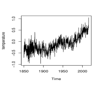
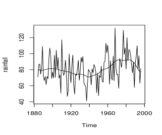
Figure 7: Left panel: deseasonalized global temperature 1850–2015 and its fitted mean-trend. Right panel: Yearly Rainfall of Tucumán Province, Argentina, 1884–1996.

We are interested in the question if the deseasonalized monthly temperature exceeds the temperature in January $1850$ by more than $c=0.15$ degrees Celsius in more than $100\Delta\%$ of the considered period. For this purpose we run the test (4.19) for the hypothesis (1.8), where the bandwidth (chosen by GCV) is $b_{n}=0.105$ and $h_{d}=0.011$ (we note again that the procedure is rather stable with respect to the choice of $h_{d}$). For the estimate (4.24) of the long-run variance $\sigma^{2}$, we use the procedure described at the beginning of this section, which yields $m=30$ and $\tau=0.202$. For a threshold $\Delta=43.4\%$ we obtain a $p$-value of $4.82\%$.

Next we investigate the same question for the sub-series from January $1850$ to December $1974$. The GCV method yields the bandwidth $b_{n}=0.135$ and we chose $h_{d}=0.013$ and $m=36$, $\tau=0.234$ for the estimate of the time-varying long-run variance (see the discussion at the beginning of this section). We find that for $\Delta=26\%$ and $c=0.15$ the $p$-value is $6.6\%$. Comparing the results for the series and sub-series shows that relevant deviations of more than $c=0.15$ degrees Celsius arise more frequently between $1975$ and $2015$. The conclusions of this short data analysis are similar to those of many authors, but by our method we are able to quantitatively describe relevant deviations. For example, if we reject the hypothesis that in less than $26\%$ of the time between January $1850$ and April $2015$ the mean function exceeds its value from January 1850 by more than $c=0.15$ degrees Celsius, the type I error of this conclusion is less or equal than $5\%$.

6.2 Rainfall data

In this example we analyze the yearly rainfall data (in millimeters) from $1884$ to $1996$ in the Tucumán Province, Argentina, which is a predominantly agriculture region. Therefore its economy well-being depends sensitively on timely rainfall. The series with a local linear estimate of the mean trend are depicted in right panel of Figure 7 (note that the range of estimated mean function is $[71.0$mm, $92.5$mm]) and it has been studied by several authors in the context of change point analysis with different conclusions. For example, the null hypothesis of no change point is rejected by the conventional CUSUM test, isotonic regression approach of Wu, Woodroofe and Mentz (2001) with $p$-value smaller than $0.1\%$, and the robust bootstrap test of Zhou (2013) with a $p$-value smaller than $2\%$. On the other hand a self-normalization method considered in Shao and Zhang (2010) reports a $p$-value about $10\%$.

Meanwhile, there is some belief that there exists a change point because of the construction of a dam near the region during $1952-1962$. As a result, a more practical question is whether the construction of the dam has a relevant influence on the economic well-being of the region via affecting the annual rainfall. To investigate this question, we are testing the hypotheses (1.8) with a threshold $\Delta=0.05$ (here we calculated $b_{n}=0.235$, $m=11$, $\tau=0.24$ and $h_{d}=0.047$ as described at the beginning of this section). For the level $c=7$ the $p$-value is $6.03\%$. In other words the hypothesis that in less than $5\%$ of the $113$ years the mean annual rainfall is at least $7$mm higher than the rainfall in the year $1880$ can not be rejected. This result indicates that the effect of the new dam on the change of the amount of rainfall is small.

7 Further discussion

We conclude this paper with a brief discussion of the extension of the proposed concept to the multivariate case and its relation to the concept of sojourn times in probability theory.

7.1 Multivariate data

The results of this paper can be extended to multivariate time series of the form

$$\mathbf{X}_{i,n}=\boldsymbol{\mu}(i/n)+\mathbf{e}_{i,n}~{},$$ (7.1)

where $\mathbf{X}_{i,n}=(X_{i,n}^{1},...,X_{i,n}^{m})^{T}$ is the $m$-dimensional vector of observations, $\boldsymbol{\mu}(i/n)=(\mu^{1}(i/n),...,\mu^{m}(i/n))^{T}$ its corresponding expectation and $(\mathbf{e}_{i,n})_{i=1\ldots,n}$ is an $m$-dimensional time series such that $\mathbf{e}_{i,n}=\boldsymbol{G}(i/n,\mathcal{F}_{i})$, where $\mathbf{G}(t,\mathcal{F}_{i})=(G_{1}(t,\mathcal{F}_{i}),...,G_{m}(t,\mathcal{F}_{i}))^{T}$ is an $m$-dimensional filter. Assume that the long run variance matrix

$$\Sigma(t)=\sum_{{i}=-\infty}^{\infty}\mbox{cov}(\boldsymbol{G}(t,\mathcal{F}_{i}),\boldsymbol{G}(t,\mathcal{F}_{0}))$$

of the error process is strictly positive and let $\|\mathbf{v}\|$ denote the Euclidean norm of an $m$-dimensional vector $\mathbf{v}$. The excess mass for the $m$-dimensional mean function is then defined as

$$\boldsymbol{T}_{c}:=\int_{0}^{1}\mathbf{1}(\|\boldsymbol{\mu}(t)-\boldsymbol{\mu}(0)\|>c)dt$$ (7.2)

and a test for the hypotheses $H_{0}:\boldsymbol{T}_{c}\leq\Delta$ versus $H_{1}:\boldsymbol{T}_{c}>\Delta$ can be developed by estimating this quantity by

$$\hat{\boldsymbol{T}}_{N,c}=\frac{1}{N}\sum_{i=1}^{N}\int_{c^{2}}^{\infty}\frac{1}{h_{d}}K_{d}\left(\frac{\|\hat{\boldsymbol{\mu}}(i/N)-\hat{\boldsymbol{\mu}}(0)\|^{2}-u}{h_{d}}\right)du,$$ (7.3)

where $\hat{\boldsymbol{\mu}}$ denote the vector of component-wise bias-corrected Jackknife estimates of the vector of regression functions.

The corresponding bootstrap test is now obtained by rejecting the null hypothesis at level $\alpha$, whenever

$$nNb_{n}h_{d}\hat{\boldsymbol{T}}_{N,c}-\Delta>q_{1-\alpha}~{},$$ (7.4)

where $q_{1-\alpha}$ is the $(1-\alpha)$-quantile of the random variable

$$\sum_{j=1}^{n}\sum_{i=1}^{N}K_{d}\left(\frac{\hat{\boldsymbol{g}}(i/N)-c^{2}}{h_{d}}\right)\left(K^{*}\left(\frac{j/n-i/N}{b_{n}}\right)-\bar{K}^{*}\left(\frac{j}{nb_{n}}\right)\right)(\nabla\hat{\boldsymbol{g}}(i/N))^{T}\hat{\Sigma}^{1/2}(j/n)\boldsymbol{V}_{j},$$ (7.5)

$\nabla\hat{\boldsymbol{g}}(u)$ is the gradient of the function $\hat{\boldsymbol{g}}(u)=\|\hat{\boldsymbol{\mu}}(u)-\hat{\boldsymbol{\mu}}(0)\|^{2}$, ${\boldsymbol{V}}_{1},{\boldsymbol{V}}_{2},\ldots$ are independent standard normally distributed $m$-dimensional random vectors and $\hat{\Sigma}(t)$ is an analogue of the long run variance matrix estimator defined in (4.24).

Under similar conditions as stated in in Assumption 2.1, 2.2, 4.1, 4.2 and in Theorem 4.1(a), an analogue of Theorem 4.3 can be proved, i.e. the bootstrap test defined by (7.4) has asymptotic level $\alpha$ and is consistent.

7.2 Estimates of excess measures related to sojourn times

The excess measures (1.12) and (1.13) based on sojourn times can easily be estimated under the assumption that the process $\{\epsilon(t)-\epsilon(0)\}_{t\in[0,1]}$ is stationary with density $f$. In this case the quantities $e_{c}$ and $p_{c,\Delta}$ can be expressed as

$$e_{c} =\mathbb{E}(S_{c})=\int\int_{0}^{1}\mathbf{1}(|\mu(t)-\mu(0)+x|>c)f(x)dtdx,$$ (7.6)

$$p_{c,\Delta} =\mathbb{P}(S_{c}>\Delta)=\mathbb{E}(\mathbb{E}(\mathbf{1}(S_{c}>\Delta)|\epsilon(t)-\epsilon(0)=x))$$ (7.7)

$$=\int\mathbf{1}\Big{(}\int_{0}^{1}\mathbf{1}(|\mu(t)-\mu(0)+x|>c)dt>\Delta\Big{)}f(x)dx,$$

and corresponding estimators are given by

$$\hat{e}_{c} =\frac{1}{Nnh_{d}}\sum_{i=1}^{n}\sum_{s=1}^{N}\int_{c}^{\infty}K_{d}\Big{(}\frac{|\hat{\mu}(s/N)-\hat{\mu}(0)+\hat{Z}(i/n)|-u}{h_{d}}\Big{)}du,$$ (7.8)

$$\hat{p}_{c,\Delta} =\frac{1}{n}\sum_{i=1}^{n}\mathbf{1}\Big{(}\frac{1}{Nh_{d}}\sum_{s=1}^{N}\int_{c}^{\infty}K_{d}\Big{(}\frac{|\hat{\mu}(s/N)-\hat{\mu}(0)+\hat{Z}(i/n)|-u}{h_{d}}\Big{)}du>\Delta\Big{)},$$ (7.9)

respectively, where $\hat{\mu}(t)-\hat{\mu}(0)$ is a consistent estimator (say a local linear) of $\mu(t)-\mu(0)$ and $\hat{Z}(t)=\hat{\epsilon}(t)-\hat{\epsilon}(0)$ denotes the corresponding residual. Statistical analysis can then be developed along the lines of this paper.
However, in the case of a non-stationary error process as considered in this paper the situation is much more complicated and we leave the development of estimators and investigation of their (asymptotic) properties for future research.

8 Proofs of main results

In this section we will prove the main results of this paper. For the sake of a simple notation we write $e_{i}:=\epsilon_{i,n}$ throughout this section, where $\epsilon_{i,n}$ is the non-stationary error process in model (1.4). Moreover, in all arguments given below $M$ denotes a sufficiently large constant which may vary from line to line. For the sake of brevity we will restrict ourselves to proofs of the results in Section 4, while the details for the proofs of the results in Section 3 are omitted as they follow by similar arguments as presented here. We will give a proof of Theorem 4.1 (deferring some of the more technical arguments to the supplementary material) and of Theorem 4.3 in this section. The proof of Theorem 4.4 can also be found in the supplementary material.

8.1 Proof of Theorem 4.1

It follows from Assumption 2.1 that there exist $k^{+}\geq 1$ roots $t_{1}^{+}<\ldots<t_{k^{+}}^{+}$ of the equation $\mu(t)=\mu(0)+c$. Define $\gamma^{+}=\min_{0\leq i\leq k^{+}}(t_{i+1}^{+}-t_{i}^{+})>0$, with the convention that $t_{0}^{+}=0$ and $t_{k^{+}+1}^{+}=1$. Recalling the definition of the statistic $\tilde{T}_{N,c}^{+}$ and the quantity $T_{N,c}^{+}$ in (4.5) and (2.6), respectively, we obtain the decomposition

$$\tilde{T}_{N,c}^{+}-T_{N,c}^{+}=\Delta_{1,N}+\Delta_{2,N},$$ (8.1)

where the random variables $\Delta_{1,N}$ and $\Delta_{1,N}$ are defined by

$$\begin{split}\Delta_{1,N}&=\frac{1}{N}\sum_{i=1}^{N}\int_{c}^{\infty}\frac{1}{h_{d}^{2}}K_{d}^{\prime}\Big{(}\frac{\mu(\frac{i}{N})-\mu(0)-u}{h_{d}}\Big{)}(\tilde{\mu}_{b_{n}}(\tfrac{i}{N})-\mu(\tfrac{i}{N})-(\tilde{\mu}_{b_{n}}(0)-\mu(0)){)}du,\\ \Delta_{2,N}&=\frac{1}{2N}\sum_{i=1}^{N}\int_{c}^{\infty}\frac{1}{h_{d}^{3}}K_{d}^{\prime\prime}\Big{(}\frac{\zeta_{i}-u}{h_{d}}\Big{)}(\tilde{\mu}_{b_{n}}(\tfrac{i}{N})-\mu(\tfrac{i}{N})-(\tilde{\mu}_{b_{n}}(0)-\mu(0)){)}^{2}du\end{split}~{}~{}~{}~{}~{}~{}$$ (8.2)

(note that we do reflect the dependence of $\Delta_{\ell,N}$ on $n$ in our notation) and $\zeta_{i}$ denotes a random variable satisfying $|\zeta_{i}-(\mu(i/N)-\mu(0))|\leq|\tilde{\mu}_{b_{n}}(i/N)-\mu(i/N)-(\tilde{\mu}_{b_{n}}(0)-\tilde{\mu}(0))|$ and $|\zeta_{i}-(\tilde{\mu}_{b_{n}}(i/N)-\tilde{\mu}_{b_{n}}(0))|\leq|\tilde{\mu}_{b_{n}}(i/N)-\mu(i/N)-(\tilde{\mu}_{b_{n}}(0)-\mu(0))|$. It is easy to see that

$$|2\Delta_{2,N}|=\Big{|}\frac{1}{N}\sum_{i=1}^{N}\frac{1}{h_{d}^{2}}K_{d}^{\prime}\Big{(}\frac{\zeta_{i}-c}{h_{d}}\Big{)}(\tilde{\mu}_{b_{n}}(i/N)-\mu(i/N)-{(}\tilde{\mu}_{b_{n}}(0)-\mu(0){)})^{2}du\Big{|}.$$ (8.3)

Recall the definition of $\pi_{n}$ in (4.8) and define

$$~{}~{}~{}~{}A_{n}=\Big{\{}\sup_{t\in[b_{n},1-b_{n}]\cup\{0\}}|\tilde{\mu}_{b_{n}}(t)-\mu(t)|\leq\pi_{n},\sup_{t\in[0,b_{n})\cup(1-b_{n},b_{n}]}|\tilde{\mu}_{b_{n}}(t)-\mu(t)|\leq b_{n}^{2}\vee\pi_{n}\Big{\}},$$ (8.4)

where we denote $\max\{a,b\}$ by $a\vee b$. By Lemma 10.3 in Section 10 of the online supplement, we have $\lim_{n\rightarrow\infty}\mathbb{P}(A_{n})=1$ and Lemma 10.1 of the online supplement yields

$$\sharp\{i:|\tilde{\mu}_{b_{n}}(i/N)-\tilde{\mu}_{b_{n}}(0)-c|\leq h_{d},|\tilde{\mu}_{b_{n}}(i/N)-\mu(i/N)-(\tilde{\mu}_{b_{n}}(0)-\mu(0))|\leq 2\pi_{n}\}$$

$$\leq\sharp\{i:|\mu(i/N)-\mu(0)-c|\leq h_{d}+2\pi_{n}\}=O(N(h_{d}+\pi_{n})^{1/(v^{+}+1)})$$ (8.5)

almost surely, where $\sharp A$ denotes the number of points in the set $A$. Observing the definition of $\zeta_{i}$ and (8.5) we obtain that the number of non-vanishing terms on the right hand side of equality (8.3) is bounded by $O(N(h_{d}+\pi_{n})^{\frac{1}{v+1}})$. Therefore the triangle inequality yields for a sufficiently large constant $M$

$$\|\Delta_{2,N}\mathbf{1}(A_{n})\|_{2}\leq M\Big{(}b_{n}^{6}+\frac{1}{nb_{n}}\Big{)}h^{-2}_{d}((h_{d}+\pi_{n})^{\frac{1}{v^{+}+1}}).$$ (8.6)

Now Proposition B.3 of Dette, Wu and Zhou (2015b) (note that $\lim_{n\rightarrow\infty}\mathbb{P}(A_{n})=1$) yields the estimate

$$\Delta_{2,N}=O_{p}\Big{(}(b_{n}^{6}+\frac{1}{nb_{n}})h^{-2}_{d}((h_{d}+\pi_{n})^{\frac{1}{v^{+}+1}}\Big{)}.$$ (8.7)

Notice that the assumptions regarding bandwidths guarantee that

$$\sqrt{nh_{d}}h_{d}^{\frac{v^{+}}{2(v^{+}+1)}}\Delta_{2,N} =o(1),\ \text{~{}~{}if ~{} $b_{n}^{v^{+}+1}/h_{d}=r\in[0,\infty)$},$$ (8.8)

$$\sqrt{nb_{n}}h_{d}^{\frac{v^{+}}{v^{+}+1}}\Delta_{2,N} =o(1),\ \text{ ~{}~{}if ~{}$b_{n}^{v^{+}+1}/h_{d}\rightarrow\infty$},$$ (8.9)

and therefore it remains to consider the term $\Delta_{1,N}$ in the decomposition (8.1).

For this purpose we recall its definition in (8.2) and obtain by an application of Lemma 10.3 of the online supplement and straightforward calculations the following decomposition

$$\Delta_{1,n} =\frac{-1}{Nh_{d}}\sum_{i=1}^{N}K_{d}\Big{(}\frac{\mu(i/N)-\mu(0)-c}{h_{d}}\Big{)}\left(\left(\tilde{\mu}_{b_{n}}(i/N)-\mu(i/N)\right)-\left(\tilde{\mu}_{b_{n}}(0)-\mu(0)\right)\right)$$

$$=I+R,$$ (8.10)

where the terms $I$ and $R$ are defined by

$$I =\frac{-1}{nNb_{n}h_{d}}\sum_{i=1}^{N}K_{d}\Big{(}\frac{\mu(\tfrac{i}{N})-\mu(0)-c}{h_{d}}\Big{)}\sum_{j=1}^{n}e_{j}\Big{(}K^{*}\Big{(}\frac{\tfrac{i}{N}-\tfrac{j}{n}}{b_{n}}\Big{)}-\bar{K}^{*}\Big{(}\frac{j}{nb_{n}}\Big{)}\Big{)},$$ (8.11)

$$R =O\Big{(}\frac{1}{Nh_{d}}\sum_{i=1}^{N}K_{d}\Big{(}\frac{\mu(\tfrac{i}{N})-\mu(0)-c}{h_{d}}\Big{)}\Big{(}b_{n}^{3}+\frac{1}{nb_{n}}\Big{)}\Big{)}.$$ (8.12)

By Lemma 10.1 of the online supplement the term $R$ is of order $O(h_{d}^{-\frac{v^{+}}{v^{+}+1}}(b_{n}^{3}+\frac{1}{nb_{n}}))$. For the investigation of the remaining term $I$, we use Proposition 5 of Zhou (2013), which shows that there exist (on a possibly richer probability space), independent stand normally distributed random variables $\{V_{i}\}_{i\in\mathbb{Z}}$, such that

$$\max_{1\leq i\leq n}|\sum_{j=1}^{i}e_{j}-\sum_{j=1}^{i}\sigma(j/n)V_{j}|=o_{p}(n^{1/4}\log^{2}n).$$ (8.13)

This representation and the summation by parts formula in equation (44) of Zhou (2010) yield

$$\sup_{t\in[0,1]}\Big{|}\sum_{j=1}^{n}e_{j}\tilde{K}^{*}\Big{(}\frac{t-j/n}{b_{n}}\Big{)}-\sum_{j={1}}^{i}\sigma(j/n)V_{j}\tilde{K}^{*}\Big{(}\frac{t-j/n}{b_{n}}\Big{)}\Big{|}=o_{p}(n^{1/4}\log^{2}n),$$ (8.14)

where we introduce the notation

$$\tilde{K}^{*}\Big{(}\frac{t-j/n}{b_{n}}\Big{)}=K^{*}\Big{(}\frac{t-j/n}{b_{n}}\Big{)}-\bar{K}^{*}\Big{(}\frac{j}{nb_{n}}\Big{)}.$$ (8.15)

Using these results in (8.11) and Lemma 10.1 of the online supplement provides an asymptotically equivalent representation of the term $I$, that is

$$|I^{\prime}-I|=o_{p}\Big{(}\frac{n^{1/4}\log^{2}n}{nb_{n}}h_{d}^{-\frac{v^{+}}{v^{+}+1}}\Big{)}.$$ (8.16)

Here

$$I^{\prime}:=\frac{-1}{nNb_{n}h_{d}}\sum_{j=1}^{n}\sum_{i=1}^{N}K_{d}\Big{(}\frac{\mu(i/N)-\mu(0)-c}{h_{d}}\Big{)}\sigma(j/n)\tilde{K}^{*}\Big{(}\frac{i/N-j/n}{b_{n}}\Big{)}V_{j}$$

is a zero mean Gaussian random variable with variance

$$\mbox{Var}(I^{\prime}) =\frac{1}{n^{2}b_{n}^{2}h_{d}^{2}}\sum_{j=1}^{n}\Big{(}\frac{1}{N}\sum_{i=1}^{N}\sigma(j/n)\tilde{K}^{*}\Big{(}\frac{i/N-j/n}{b_{n}}\Big{)}K_{d}\Big{(}\frac{\mu(i/N)-\mu(0)-c}{h_{d}}\Big{)}\Big{)}^{2}$$

$$=\frac{1}{n^{2}b_{n}^{2}h_{d}^{2}}\sum_{j=1}^{n}\Big{(}\int_{0}^{1}\sigma(j/n)\tilde{K}^{*}\Big{(}\frac{t-j/n}{b_{n}}\Big{)}K_{d}\Big{(}\frac{\mu(t)-\mu(0)-c}{h_{d}}\Big{)}dt\Big{)}^{2}+\beta_{n}$$

$$:=\bar{\alpha}_{n}+\beta_{n},$$ (8.17)

and the last two equalities define the quantities $\bar{\alpha}_{n}$ and $\beta_{n}$ in an obvious manner. Observing the estimates

$$\frac{1}{N}\sum_{i=1}^{N}\sigma(\frac{j}{n})\tilde{K}^{*}\Big{(}\frac{i/N-j/n}{b_{n}}\Big{)}K_{d}\Big{(}\frac{\mu(i/N)-\mu(0)-c}{h_{d}}\Big{)}-$$

$$\int_{0}^{1}\sigma(\frac{j}{n})\tilde{K}^{*}\Big{(}\frac{t-j/n}{b_{n}}\Big{)}K_{d}\Big{(}\frac{\mu(t)-\mu(0)-c}{h_{d}}\Big{)}dt=O\Big{(}(\frac{1}{Nb_{n}}+\frac{1}{Nh_{d}})(b_{n}\wedge h_{d}^{\frac{1}{v^{+}+1}})\Big{)},$$

$$\frac{1}{n^{2}b_{n}^{2}h_{d}^{2}}\sum_{j=1}^{n}\Big{(}\int_{0}^{1}\sigma(j/n)\tilde{K}^{*}\Big{(}\frac{t-j/n}{b_{n}}\Big{)}K_{d}\Big{(}\frac{\mu(t)-\mu(0)-c}{h_{d}}\Big{)}dt\Big{)}=O\Big{(}\frac{h_{d}^{\frac{-v^{+}}{v^{+}+1}}}{nb_{n}h_{d}}\Big{)},$$

we have that

$$\beta_{n}=\frac{h_{d}^{\frac{-v^{+}}{v^{+}+1}}}{nb_{n}h_{d}}\Big{(}\frac{1}{Nb_{n}}+\frac{1}{Nh_{d}}\Big{)}(b_{n}\wedge h_{d}^{\frac{1}{v^{+}+1}})+\Big{(}(\frac{1}{Nb_{n}}+\frac{1}{Nh_{d}})(b_{n}\wedge h_{d}^{\frac{1}{v^{+}+1}})\Big{)}^{2},$$ (8.18)

where $a\wedge b:=\min(a,b)$.

For the calculation of $\bar{\alpha}_{n}$ we note that

$$\bar{K}^{*}\Big{(}\frac{j/n}{b_{n}}\Big{)}K^{*}\Big{(}\frac{t-j/n}{b_{n}}\Big{)}K_{d}\Big{(}\frac{\mu(t)-\mu(0)-c}{h_{d}}\Big{)}=0.$$ (8.19)

for sufficiently large $n$. This statement follows because by Lemma 10.1 of the online supplement the third factor vanishes outside of (shrinking) neighbourhoods ${\cal U}_{1},\ldots,{\cal U}_{k^{+}}$ of the points $t_{1}^{+},\ldots,t_{k^{+}}^{+}$ with Lebesgue measure of order $h_{d}^{\frac{1}{v_{l}+1}}$, ($1\leq l\leq k^{+}$). Consequently, the product of the first and second factor vanishes, wheneever the point $j/n$ is not an element of the set

$$\big{\{}s+t~{}\big{|}~{}t\in\cup_{j=1}^{k^{+}}{\cal U}_{j}~{};s\in[-b_{n},b_{n}]\big{\}}.$$

However, if $n$ is sufficiently large the intersection of this set with the interval $[0,b_{n}]$, is empty. Consequently, for sufficiently large $n$ there exists no pair $(t,j/n)$ such that all factors in (8.19) different from zero.
Therefore, we obtain (recalling the notation of $\tilde{K}^{*}$ in (8.15))

$$\bar{\alpha}_{n}=\alpha_{n}+\tilde{\alpha}_{n},$$ (8.20)

where

$$\alpha_{n} =\frac{1}{n^{2}b_{n}^{2}h_{d}^{2}}\sum_{j=1}^{n}\Big{(}\int_{0}^{1}\sigma(j/n)K^{*}\Big{(}\frac{t-j/n}{b_{n}}\Big{)}K_{d}\Big{(}\frac{\mu(t)-\mu(0)-c}{h_{d}}\Big{)}dt\Big{)}^{2},$$ (8.21)

$$\tilde{\alpha}_{n} =\frac{1}{n^{2}b_{n}^{2}h_{d}^{2}}\sum_{j=1}^{n}\Big{(}\int_{0}^{1}\sigma(j/n)\bar{K}^{*}\Big{(}\frac{j/n}{b_{n}}\Big{)}K_{d}\Big{(}\frac{\mu(t)-\mu(0)-c}{h_{d}}\Big{)}dt\Big{)}^{2}.$$ (8.22)

In the supplementary material we will show that

$$\alpha_{n} =\left\{\begin{array}[]{cl}{h_{d}^{\frac{-2v^{+}}{v^{+}+1}}}({nb_{n}})^{-1}\sigma_{1}^{2,+}&\mbox{ if }b^{v^{+}+1}_{n}/h_{d}\rightarrow\infty\\ &\\ {h_{d}^{\frac{1}{v^{+}+1}}}({nh_{d}^{2}})^{-1}\rho_{1}^{2,+}&\mbox{ if }b^{v^{+}+1}_{n}/h_{d}\rightarrow r\in[0,\infty)\end{array}\right.$$ (8.26)

$$\tilde{\alpha}_{n} =\left\{\begin{array}[]{cl}{h_{d}^{\frac{-2v^{+}}{v^{+}+1}}}({nb_{n}})^{-1}\sigma_{2}^{2,+}&\mbox{ if }b^{v^{+}+1}_{n}/h_{d}\rightarrow\infty\\ &\\ {h_{d}^{\frac{1}{v^{+}+1}}}({nh_{d}^{2}})^{-1}\rho_{2}^{2,+}&\mbox{ if }b^{v^{+}+1}_{n}/h_{d}\rightarrow r\in[0,\infty)\end{array}\right.~{}.$$ (8.30)

where $\sigma_{1}^{2,+}$, $\sigma_{2}^{2,+}$, $\rho_{1}^{2,+}$ and $\rho_{2}^{2,+}$ are defined in Theorem 4.1. The assertion now follows from (8.1), (8.8), (8.9), (8.1) and (8.16) observing that the random variable $I^{\prime}$ is normally distributed, where the (asymptotic) variance can be obtained from (8.1), (8.18), (8.20), (8.26) and (8.30). $\Box$

8.2 Proof of Theorem 4.3

We have to distinguish two cases:

(1) The equation $\mu(t)-\mu(0)=c$ has at least one solution. Recall the definition of the quantity $I^{\prime}$ in (4.17), then it follows from the proof of Theorem 4.1, that

$$\mbox{Var}(\sqrt{nb_{n}}h_{d}^{\frac{v^{+}}{v^{+}+1}}I^{\prime})=\sigma^{{2,+}}_{1}+\sigma^{{2,+}}_{2}+o(1),$$ (8.31)

where $\sigma^{{2,+}}_{1}$ and $\sigma^{{2,+}}_{2}$ are defined in (4.10) and (4.11), respectively. Note that $\mbox{Var}(I^{\prime})=\frac{1}{n^{2}N^{2}b^{2}_{n}h^{2}_{d}}\tilde{V}$, where

$$\tilde{V}=\sum_{j=1}^{n}\sigma^{2}(j/{n})\Big{(}\sum_{i=1}^{N}K_{d}\Big{(}\frac{\mu(i/N)-\mu(0)-c}{h_{d}}\Big{)}\Big{(}K^{*}\Big{(}\frac{i/N-j/n}{b_{n}}\Big{)}-\bar{K}^{*}\Big{(}\frac{j}{nb_{n}}\Big{)}\Big{)}\Big{)}^{2}.$$

At the end of this proof we will show that

$$\frac{(\sqrt{nb_{n}}h_{d}^{\frac{v^{+}}{v^{+}+1}})^{2}}{n^{2}N^{2}b^{2}_{n}h^{2}_{d}}(\tilde{V}-\bar{V})=o(1),$$ (8.32)

which implies that

$$\lim_{n\to\infty}{\sqrt{nb_{n}}h_{d}^{\frac{v^{+}}{v^{+}+1}}}q^{+}_{1-\alpha}/({nNb_{n}h_{d}})=\Phi^{-1}(1-\alpha)\sqrt{\sigma_{1}^{{2,+}}+\sigma_{2}^{{2,+}}}.$$ (8.33)

Observing the identity

$$\mathbb{P}\big{(}nNb_{n}h_{d}\big{(}\tilde{T}_{N,c}^{+}-\Delta\big{)}>q^{+}_{1-\alpha}\big{)}$$ (8.34)

$$=\mathbb{P}\left(\frac{\sqrt{nb_{n}}h_{d}^{\frac{v^{+}}{v^{+}+1}}\big{(}\tilde{T}_{N,c}^{+}-T_{c}^{+}\big{)}}{\sqrt{\sigma_{1}^{{2,+}}+\sigma_{2}^{{2,+}}}}>\frac{\frac{\sqrt{nb_{n}}h_{d}^{\frac{v^{+}}{v^{+}+1}}}{nNb_{n}h_{d}}q^{+}_{1-\alpha}+\sqrt{nb_{n}}h_{d}^{\frac{v^{+}}{v^{+}+1}}(\Delta-T_{c}^{+})}{\sqrt{\sigma_{1}^{{2,+}}+\sigma_{2}^{{2,+}}}}\right)~{}$$

the assertion now follows from (8.33) and Theorem 4.1, which shows that the random variable

$$\frac{\sqrt{nb_{n}}h_{d}^{\frac{v^{+}}{v^{+}+1}}\big{(}\tilde{T}_{N,c}^{+}-T_{c}^{+}\big{)}}{\sqrt{\sigma_{1}^{{2,+}}+\sigma_{2}^{{2,+}}}}$$

converges weakly to a standard normal distribution.

It remains to prove (8.32), which is a consequence of the following observations

• $\hat{\sigma}(t^{+}_{l})=\sigma(t^{+}_{l})(1+o(1))$, uniformly with respect to $l=1,\ldots,k^{+}$.

• The bandwidth condition $\pi_{n}/h_{d}=o(1)$, Proposition 2.1 and similar arguments as (8.5) show

  $$K_{d}\Big{(}\tfrac{\mu(\frac{i}{N})-\mu(0)-c}{h_{d}}\Big{)}-K_{d}\Big{(}\tfrac{\tilde{\mu}_{b_{n}}(\frac{i}{N})-\tilde{\mu}_{b_{n}}(0)-c}{h_{d}}\Big{)}=O\Big{(}\sum_{{\{l:v_{l}^{+}=v^{+}\}}}\mathbf{1}\big{(}\big{|}\tfrac{i}{N}-t^{+}_{l}\big{|}\leq h_{d}^{\tfrac{1}{v^{+}+1}}\big{)}\tfrac{\pi_{n}}{h_{d}}\Big{)},$$

  where $\pi_{n}$ is defined in Theorem 4.1.

This completes the proof of Theorem 4.3 in the case that there exist in fact roots of the equation $\mu(t)-\mu(0)=c$.

(2) The equation $\mu(t)-\mu(0)=c$ has no solutions. In this case we have $\mu(t)-\mu(0)<c$ where $c>0$. Note that for two sequences of measurable sets $U_{n}$ and $V_{n}$ such that $\mathbb{P}(U_{n})\rightarrow 1$ and $\mathbb{P}(U_{n}\cap V_{n})\rightarrow u\in(0,1)$, we have $\mathbb{P}(V_{n})\rightarrow u$. Consequently, as the set $A_{n}$ defined in (8.4) satisfies $\mathbb{P}(A_{n})\rightarrow 1$ the assertion of the theorem follows from

$$\lim_{n\rightarrow\infty}\mathbb{P}(nNb_{n}h_{d}(\tilde{T}_{N,c}^{+}-\Delta)>q_{1-\alpha}^{+},A_{n},\mu(t)-\mu(0)<c)=0.$$ (8.35)

However, under the event $A_{n}$ and $\mu(t)-\mu(0)<c$ we have $q_{1-\alpha}^{+}=0$ and $\tilde{T}_{N,c}^{+}=0$, if $n$ is sufficiently large. Thus (8.35) is obvious (note that $0<\Delta<1$), which finishes the proof in the case where the equation $\mu(t)-\mu(0)=c$ has in fact no roots. $\Box$

Appendix 
 
In this section we will provide technical details for the proof of Theorem 4.1 and a proof of Theorem 4.4. Recall that we use the notation $e_{i}:=\epsilon_{i,n}$ throughout this section, where $\epsilon_{i,n}$ is the nonstationary error process in model (1.4). Moreover, in all arguments given below $M$ denotes a sufficiently large constant which may vary from line to line.

9 Proof of of Theorem 4.1 and 4.4

Proof of Theorem 4.1. Following the arguments of the main article, it remains to show (8.26) and (8.30) to complete the proof of Theorem 4.1.

Proof of (8.26): By Lemma 10.1 with $m$ replaced by $\mu(0)+c$, there exists a small positive number $0<\epsilon<\gamma^{+}/4$ such that when $n$ is sufficiently large, we have

$$\alpha_{n} =\frac{1}{n^{2}b_{n}^{2}h_{d}^{2}}\sum_{j=1}^{n}\Big{(}\sum_{l=1}^{k^{+}}\int_{t_{l}^{+}-\epsilon}^{t_{l}^{+}+\epsilon}\sigma(j/n)K^{*}\Big{(}\frac{t-j/n}{b_{n}}\Big{)}K_{d}\Big{(}\frac{\mu(t)-\mu(0)-c}{h_{d}}\Big{)}dt\Big{)}^{2}$$

$$=\frac{1}{n^{2}b_{n}^{2}h_{d}^{2}}\sum_{j=1}^{n}\sum_{l=1}^{k^{+}}\Big{(}\int_{t_{l}^{+}-\epsilon}^{t_{l}^{+}+\epsilon}\sigma(j/n)K^{*}\Big{(}\frac{t-j/n}{b_{n}}\Big{)}K_{d}\Big{(}\frac{\mu(t)-\mu(0)-c}{h_{d}}\Big{)}dt\Big{)}^{2}$$

$$=\frac{1}{n^{2}b_{n}^{2}h_{d}^{2}}\sum_{j=1}^{n}\sum_{l=1}^{k^{+}}\alpha^{2}_{n,l,j},$$ (8.1)

where the last equation defines the quantities $\alpha_{n,l,j}^{2}$ in an obvious manner. We now calculate $\alpha_{n}$ for the two bandwidth conditions in (8.26).

(i) We begin with the case $b^{v^{+}+1}_{n}/h_{d}\rightarrow\infty$, which means $b^{v^{+}_{l}+1}_{n}/h_{d}\rightarrow\infty$ for $l=1,\dots,k$. By Lemma 10.1 there exists a sufficiently large constant $M$ such that

$$\ \ \ \ \ \ \alpha_{n,l,j}=\int_{t_{l}^{+}-Mh_{d}^{\frac{1}{v^{+}_{l}+1}}}^{t_{l}^{+}+Mh_{d}^{\frac{1}{v^{+}_{l}+1}}}\sigma(t_{l}^{+})K^{*}\Big{(}\frac{t-j/n}{b_{n}}\Big{)}K_{d}\Big{(}\frac{\mu(t)-\mu(0)-c}{h_{d}}\Big{)}dt\Big{(}1+O\Big{(}h_{d}^{\frac{1}{v^{+}_{l}+1}}\Big{)}\Big{)}.$$ (8.2)

Observing the fact that the kernel $K_{d}(\cdot)$ is bounded and continuous we obtain by a Taylor expansion of $\mu(t)-\mu(0)-c$ around $t_{l}^{+}$,

$$\big{|}\alpha_{n,l,j}-\alpha_{n,l,j}^{*}\big{|}=O\Big{(}h_{d}^{\frac{2}{v^{+}_{l}+1}}\mathbf{1}(|j/n-t^{+}_{l}|\leq 2b_{n})\Big{)}$$ (8.3)

uniformly with respect to $t\in[0,1]$, where

$$\alpha_{n,l,j}^{*}=\int_{t_{l}^{+}-Mh_{d}^{\frac{1}{v^{+}_{l}+1}}}^{t_{l}^{+}+Mh_{d}^{\frac{1}{v^{+}_{l}+1}}}\sigma(t_{l}^{+})K^{*}\Big{(}\frac{t-j/n}{b_{n}}\Big{)}K_{d}\Big{(}\frac{\mu^{(v^{+}_{l}+1)}(t^{+}_{l})(t-t^{+}_{l})^{v^{+}_{l}+1}}{(v^{+}_{l}+1)!h_{d}}\Big{)}dt.$$

Substituting $t=t_{l}^{+}+z\big{|}{h_{d}(v^{+}_{l}+1)!}/{\mu^{(v^{+}_{l}+1)}(t_{l}^{+})}\big{|}^{\frac{1}{v^{+}_{l}+1}}$, observing the symmetry of $K_{d}(\cdot)$ and using a Taylor expansion shows that

$$\alpha_{n,l,j}^{*} =\Big{|}\frac{(v^{+}_{l}+1)!h_{d}}{\mu^{(v^{+}_{l}+1)}(t^{+}_{l})}\Big{|}^{\frac{1}{v^{+}_{l}+1}}\Big{(}\int K_{d}(z^{v^{+}_{l}+1})dz\Big{)}\sigma(t^{+}_{l})K^{*}\Big{(}\frac{t^{+}_{l}-j/n}{b_{n}}\Big{)}$$ (8.4)

$$~{}~{}~{}~{}~{}~{}~{}+O\Big{(}{h_{d}^{\frac{2}{v^{+}_{l}+1}}}({b_{n}})^{-1}\mathbf{1}(|j/n-t^{+}_{l}|\leq 2b_{n})\Big{)},$$

where we have used the fact that $\int zK_{d}(z^{v^{+}_{l}+1})dz<\infty$ since $K_{d}(\cdot)$ has a compact support. Equations (8.2)–(8.4) and the condition $\frac{b_{n}^{v^{+}+1}}{h_{d}}\rightarrow\infty$ now give

$$\alpha_{n} =\frac{1}{n^{2}b_{n}^{2}h_{d}^{2}}\sum_{l=1}^{k}\sum_{j=1}^{n}\Big{(}\Big{(}\int K_{d}(z^{v_{l}^{+}+1})dz\Big{)}\sigma(t^{+}_{l})\Big{|}\frac{(v^{+}+1)!h_{d}}{\mu^{(v^{+}+1)}(t_{l}^{+})}\Big{|}^{\frac{1}{v^{+}+1}}K^{*}\Big{(}\frac{t_{l}^{+}-j/n}{b_{n}}\Big{)}\Big{)}^{2}$$

$$~{}~{}~{}~{}~{}~{}~{}~{}~{}~{}~{}~{}~{}~{}~{}\times\left(1+O\big{(}{h_{d}^{\frac{1}{v^{+}+1}}}{b_{n}}^{-1}\mathbf{1}(|j/n-t^{+}_{l}|\leq 2b_{n})\big{)}\right)$$

$$=\sum_{l=1}^{k}\frac{h_{d}^{\frac{-2v_{l}^{+}}{v_{l}^{+}+1}}}{nb_{n}}\Big{(}\int K_{d}(z^{v_{l}^{+}+1})dz\Big{)}^{2}((v_{l}^{+}+1)!)^{\frac{2}{v_{l}^{+}+1}}\Big{(}\frac{\sigma(t_{l}^{+})}{|\mu^{(v_{l}^{+}+1)}(t_{l}^{+})|^{\frac{1}{v^{+}_{l}+1}}}\Big{)}^{2}\int(K^{*}(x))^{2}dx$$

$$~{}~{}~{}~{}~{}~{}~{}~{}~{}~{}~{}~{}~{}~{}~{}\times\big{(}1+O\big{(}{(}nb_{n}{)}^{-1}+h_{d}^{\frac{1}{v^{+}_{l}+1}}/b_{n}\big{)}\big{)}$$

$$={h_{d}^{\frac{-2v^{+}}{v^{+}+1}}}({nb_{n}})^{-1}\sigma_{1}^{2,+}\big{(}1+o(1)\big{)}$$

which proves (8.26) in the case $b^{v^{+}+1}_{n}/h_{d}\rightarrow\infty$.

Next we turn to the case $b_{n}/h_{d}^{\frac{1}{v^{+}+1}}\rightarrow c\in[0,\infty)$, introduce the notation $\alpha_{n,l}=\frac{1}{n^{2}b_{n}^{2}h_{d}^{2}}\sum_{j=1}^{n}\alpha^{2}_{n,l,j}$ and note that

$$\alpha_{n}=\sum_{l=1}^{k}\alpha_{n,l}.$$ (8.5)

Define $c_{l}=b_{n}^{v^{+}_{l}+1}/h_{d}$ for $l\in\{1,\ldots,k^{+}\}$. For those $l$ satisfying $c_{l}\rightarrow\infty$, we have already shown that

$$\alpha_{n,l}=\frac{h_{d}^{\frac{-2v^{+}_{l}}{v^{+}_{l}+1}}}{nb_{n}}=o\Big{(}\frac{h_{d}^{\frac{1}{v^{+}_{l}+1}}}{nh_{d}^{2}}\Big{)}=o\Big{(}\frac{h_{d}^{\frac{1}{v^{+}+1}}}{nh_{d}^{2}}\Big{)}.$$ (8.6)

In the following discussion we prove that for those $l$, for which $c_{l}$ does not converge to infinity, the quantity $\alpha_{n,l}$ is exactly of order $O({h_{d}^{\frac{1}{v^{+}_{l}+1}}}({nh_{d}^{2}})^{-1})$. For this purpose define

$$\alpha^{\prime}_{n,l}=\frac{1}{nb_{n}^{2}h_{d}^{2}}\int_{0}^{1}\big{(}G(t^{+}_{l},s,b_{n},h_{d})\big{)}^{2}ds.$$ (8.7)

where

$$G(t^{+}_{l},s,b_{n},h_{d})=\int_{t^{+}_{l}-\epsilon}^{t_{l}^{+}+\epsilon}\sigma(s)K^{*}\Big{(}\frac{t-s}{b_{n}}\Big{)}K_{d}\Big{(}\frac{\mu(t)-\mu(0)-c}{h_{d}}\Big{)}dt.$$

It follows from a Taylor expansion and an approximation by a Riemann sum that

$$|\alpha_{n,l}-\alpha_{n,l}^{\prime}|\leq\frac{1}{nb_{n}^{2}h_{d}^{2}}\sum_{j=1}^{n}\frac{1}{n^{2}}\sup_{\frac{j-1}{n}\leq s\leq\frac{j}{n}}\left|G(t^{+}_{l},s,b_{n},h_{d})\right|\Big{|}\frac{\partial}{\partial s}G(t^{+}_{l},s,b_{n},h_{d})\Big{|}.$$ (8.8)

The terms in this sum can be estimated by an application of Lemma 10.1, that is

$$\sup_{\frac{j-1}{n}<s\leq\frac{j}{n}}\left|G(t^{+}_{l},s,b_{n},h_{d})\right| \leq C\lambda\left({\cal D}_{lj}\right),$$ (8.9)

$$\sup_{\frac{j-1}{n}<s\leq\frac{j}{n}}\Big{|}\frac{\partial}{\partial s}G_{j}(t^{+}_{l},s,b,h_{d})\Big{|} \leq C\lambda\left({\cal D}_{lj}\right)/b_{n},$$ (8.10)

where

$${\cal D}_{lj}=\Big{(}\frac{j-1}{n}-b_{n},\frac{j+1}{n}+b_{n}\Big{)}\cap\Big{(}t^{+}_{l}-Mh_{d}^{\frac{1}{v_{l}^{+}+1}},t^{+}_{l}+Mh_{d}^{\frac{1}{v_{l}^{+}+1}}\Big{)}~{},$$

$M$ and $C$ are sufficiently large constants and $\lambda(\cdot)$ denotes the Lebesgue measure. Straightforward calculations show that the number of indices $j$ such that the set ${\cal D}_{lj}$ is not empty is of order $O(nh_{d}^{\frac{1}{v^{+}_{l}+1}})$, while the Lebesgue measure in (8.9) and of (8.10) is of order $O(b_{n})$ and $O(1)$, respectively. Combining these facts we obtain

$$\alpha_{n,l}=\alpha_{n,l}^{\prime}+O\Big{(}nh_{d}^{\frac{1}{v^{+}_{l}+1}}b_{n}\frac{1}{n^{3}b_{n}^{2}h_{d}^{2}}\Big{)}$$ (8.11)

(for all $l=1,\ldots,k^{+}$ such that $c_{l}<\infty$). As the function $\sigma$ is strictly positive on a compact set it follows that

$$\alpha_{n,l}^{\prime}=\alpha_{n,l}^{\prime\prime}\Big{(}1+O\Big{(}b_{n}+h_{d}^{\frac{1}{v^{+}_{l}+1}}\Big{)}\Big{)},$$ (8.12)

where the quantity $\alpha_{n,l}^{\prime\prime}$ is defined as $\alpha_{n,l}^{\prime}$ in (8.7) replacing the $\sigma(s)$ by $\sigma(t^{+}_{l})$. Define

$$\alpha_{n,l}^{\prime\prime\prime}=\frac{\sigma^{2}(t^{+}_{l})}{nb_{n}^{2}h_{d}^{2}}\int_{0}^{1}\Big{(}\int_{t^{+}_{l}-\epsilon}^{t^{+}_{l}+\epsilon}K^{*}\Big{(}\frac{t-s}{b_{n}}\Big{)}K_{d}\Big{(}\frac{\mu^{(v^{+}_{l}+1)}(t^{+}_{l})(t-t^{+}_{l})^{v^{+}_{l}+1}}{(v^{+}_{l}+1)!h_{d}}\Big{)}dt\Big{)}^{2}ds$$ (8.13)

and note that the only difference between $\alpha_{n,l}^{\prime\prime}$ and $\alpha_{n,l}^{\prime\prime\prime}$ is the term inside $K_{d}(\cdot)$. A Taylor expansion around $t^{+}_{l}$ yields

$$\frac{\mu(t)-\mu(0)-c}{h_{d}}=\frac{\mu^{(v_{l}^{+}+1)}(t_{l}^{*})(t-t_{l}^{+})^{v_{l}^{+}+1}}{(v_{l}^{+}+1)!h_{d}}$$

for some $t_{l}^{*}\in[t_{l}\wedge t^{*}_{l},t_{l}\vee t^{*}_{l}]$ and the mean value theorem gives

$$K_{d}\Big{(}\frac{\mu(t)-\mu(c)-c}{h_{d}}\Big{)}-K_{d}\Big{(}\frac{\mu^{(v^{+}_{l}+1)}(t^{+}_{l})(t-t^{+}_{l})^{v^{+}_{l}+1}}{(v^{+}_{l}+1)!h_{d}}\Big{)}$$

$$=K_{d}^{\prime}\Big{(}\frac{((1-\theta_{l})\mu^{(v_{l}^{+}+1)}(t_{l})+\theta_{l}\mu^{(v^{+}_{l}+1)}(t_{l}^{*}))(t-t^{+}_{l})^{v^{+}_{l}+1}}{(v^{+}_{l}+1)!h_{d}}\Big{)}\frac{(\mu^{(v^{+}_{l}+1)}(t_{l}^{*})-\mu^{(v^{+}_{l}+1)}(t_{l}))(t-t^{+}_{l})^{v^{+}_{l}+1}}{(v^{+}_{l}+1)!h_{d}}$$ (8.14)

for some $\theta_{l}\in[-1,1]$. Then similar arguments as used in the derivation of (8.11) show that

$$\alpha_{n,l}^{\prime\prime\prime}-\alpha_{n,l}^{\prime\prime}=O\Big{(}{h_{d}^{-\frac{2v^{+}_{l}}{v^{+}_{l}+1}}}{n}^{-1}\Big{)}.$$ (8.15)

On the other hand, further expanding the squared term of (8.13) yields that

$$\alpha^{\prime\prime\prime}_{n,l}=\frac{\sigma^{2}(t^{+}_{l})}{nb_{n}^{2}h_{d}^{2}}\int_{0}^{1}\int_{t^{+}_{l}-\epsilon}^{t^{+}_{l}+\epsilon}\int_{t^{+}_{l}-\epsilon}^{t^{+}_{l}+\epsilon}K^{*}\Big{(}\frac{t-s}{b_{n}}\Big{)}K_{d}\Big{(}\frac{\mu^{(v^{+}_{l}+1)}(t^{+}_{l})(t-t^{+}_{l})^{v^{+}_{l}+1}}{(v^{+}_{l}+1)!h_{d}}\Big{)}$$

$$\times K^{*}\Big{(}\frac{v-s}{b_{n}}\Big{)}K_{d}\Big{(}\frac{\mu^{(v^{+}_{l}+1)}(t^{+}_{l})({v}-t^{+}_{l})^{v^{+}_{l}+1}}{(v^{+}_{l}+1)!h_{d}}\Big{)}dvdtds.$$ (8.16)

For $t,v$ satisfying $|t-t^{+}_{l}|=O(\min\{b_{n},h_{d}^{\frac{1}{v^{+}_{l}+1}}\})$, $|v-t_{l}|=O(\min\{b_{n},h_{d}^{\frac{1}{v^{+}_{l}+1}}\})$, straightforward calculations show

$$\int_{0}^{1}K^{*}\Big{(}\frac{t-s}{b_{n}}\Big{)}K^{*}\Big{(}\frac{v-s}{b_{n}}\Big{)}ds=b_{n}\int_{-\infty}^{\infty}K^{*}\Big{(}u\Big{)}K^{*}\Big{(}\frac{v-t}{b_{n}}+u\Big{)}du.$$ (8.17)

To move forward, we introduce the notation

$$z_{1}=(t-t^{+}_{l})\Big{|}\tfrac{\mu^{(v^{+}_{l}+1)}(t^{+}_{l})}{h_{d}(v^{+}_{l}+1)!}\Big{|}^{\frac{1}{v^{+}_{l}+1}},~{}z_{2}=(v-t^{+}_{l})\Big{|}\frac{\mu^{(v^{+}_{l}+1)}(t^{+}_{l})}{h_{d}(v^{+}_{l}+1)!}\Big{|}^{\tfrac{1}{v^{+}_{l}+1}},~{}\theta(v^{+}_{l},h_{d})=\Big{|}\tfrac{h_{d}(v^{+}_{l}+1)!}{\mu^{(v^{+}_{l}+1)}(t^{+}_{l})}\Big{|}^{\frac{1}{v^{+}_{l}+1}}~{}.$$

By a change of variables and (8.17), we now obtain

$$\alpha_{n,l}^{\prime\prime\prime} =\frac{\sigma^{2}(t_{l}^{+})\theta(v^{+}_{l},h_{d})^{2}}{nb_{n}h_{d}^{2}}\int\int\int K^{*}(u)K^{*}\Big{(}u+\frac{1}{b_{n}}\theta(v^{+}_{l},h_{d})(z_{2}-z_{1})\Big{)}$$

$$~{}~{}\times K_{d}(z_{1}^{v^{+}_{l}+1})K_{d}(z_{2}^{v^{+}_{l}+1})dz_{1}dz_{2}du$$

$$= \frac{\sigma^{2}(t^{+}_{l})}{nh_{d}^{2}}h_{d}^{\frac{1}{v^{+}_{l}+1}}\Big{|}\frac{(v^{+}_{l}+1)!}{\mu^{(v^{+}_{l}+1)}(t^{+}_{l})}\Big{|}^{\frac{1}{v^{+}_{l}+1}}\int\int\int K^{*}(u)K^{*}(v)K_{d}(z_{1}^{v^{+}_{l}+1})$$

$$~{}~{}\times K_{d}\Big{(}\Big{(}z_{1}+c_{l}\Big{|}\frac{(v^{+}_{l}+1)!}{\mu^{(v^{+}_{l}+1)}(t^{+}_{l})}\Big{|}^{\frac{-1}{v^{+}_{l}+1}}(v-u)\Big{)}^{v_{l}^{+}+1}\Big{)}dudvdz_{1}$$ (8.18)

Finally, combining (8.11), (8.12) and (8.15) we have that

$$\alpha_{n,l}=\alpha_{n,l}^{\prime\prime\prime}\Big{(}1+b_{n}+\frac{1}{nb_{n}}+h_{d}^{\frac{1}{v^{+}_{l}+1}}\Big{)}~{},$$ (8.19)

and, observing that $h_{d}^{\frac{1}{v^{+}_{l}+1}}=o(h_{d}^{\frac{1}{v^{+}+1}})$ whenever $v^{+}_{l}<v^{+}$, we obtain from (8.5)

$$\alpha_{n} =\frac{|h_{d}(v^{+}+1)!|^{\frac{1}{v^{+}+1}}}{nh_{d}^{2}}\sum_{\{l:v^{+}_{l}=v^{+}\}}\frac{\sigma^{2}(t^{+}_{l})}{|\mu^{(v^{+}+1)}(t^{+}_{l})|^{\frac{1}{v^{+}+1}}}\int\int\int K^{*}(u)K^{*}(v)K_{d}(z_{1}^{v^{+}+1})$$

$$\times K_{d}\Big{(}\Big{(}z_{1}+r\Big{|}\frac{(v^{+}+1)!}{\mu^{(v^{+}+1)}(t^{+}_{l})}\Big{|}^{\frac{-1}{v^{+}+1}}(v-u)\Big{)}^{v^{+}+1}\Big{)}dudvdz_{1}(1+o(1))~{},$$

which proves (8.26) in the case $b^{v^{+}+1}_{n}/h_{d}\rightarrow r\in[0,\infty)$.

Proof of (8.30). Recalling the definition of $\tilde{\alpha}_{n}$ in (8.22) we obtain by straightforward calculations and a Taylor expansion

$$\tilde{\alpha}_{n}=\frac{\sigma^{2}(0)}{nb_{n}h_{d}^{2}}\int_{0}^{1}(\bar{K}^{*}(t))^{2}dt\Big{(}\int_{0}^{1}K_{d}\Big{(}\frac{\mu(t)-\mu(0)-c}{h_{d}}\Big{)}dt\Big{)}^{2}\Big{(}1+O\Big{(}b_{n}+\frac{1}{nb_{n}}\Big{)}\Big{)}.$$ (8.20)

Similar (but easier) arguments as used in the derivation of (8.3) and (8.4) show

$$\int_{0}^{1}K_{d}\Big{(}\frac{\mu(t)-\mu(0)-c}{h_{d}}\Big{)}dt= |h_{d}(v^{+}+1)!|^{\frac{1}{v^{+}+1}}$$

$$\times \sum_{\{l:v^{+}_{l}=v^{+}\}}|\mu^{(v^{+}+1)}(t^{+}_{l})|^{-\frac{1}{v^{+}+1}}\int K_{d}(z^{v^{+}+1})dz(1+o(1)),$$ (8.21)

which gives

$$\tilde{\alpha}_{n} =\frac{\sigma^{2}(0)h_{d}^{\frac{-2v^{+}}{v^{+}+1}}((v^{+}+1)!)^{\frac{2}{v^{+}+1}}}{nb_{n}}\int_{0}^{1}(\bar{K}^{*}(t))^{2}dt$$

$$\times\Big{(}\sum_{\{l:v^{+}_{l}=v^{+}\}}|\mu^{(v^{+}+1)}(t^{+}_{l})|^{-\frac{1}{v^{+}+1}}\int K_{d}(z^{v^{+}+1})dz\Big{)}^{2}(1+o(1)).$$

Consequently, if $b^{v^{+}+1}_{n}/h_{d}\rightarrow\infty$ we have

$$\tilde{\alpha}_{n}=\frac{h_{d}^{\frac{-2v^{+}}{v^{+}+1}}}{nb_{n}}\sigma_{2}^{2,+}(1+o(1)).$$

where $\sigma_{2}^{2,+}$ is defined by (4.11). This proves the statement (8.30) in the case $b^{v^{+}+1}_{n}/h_{d}\rightarrow\infty$, while the second case follows by similar arguments observing that we have

$$nh_{d}^{\frac{v^{+}}{v^{+}+1}+1}\frac{h_{d}^{-\frac{2v^{+}}{v^{+}+1}}}{nb_{n}}=r^{-1}$$

if $b^{v^{+}+1}_{n}/h_{d}\rightarrow r^{v^{+}+1}\in[0,\infty)$.

Proof of Theorem 4.4. Define $\tilde{S}_{k,r}=\sum_{i=k\vee 1}^{r\wedge n}e_{i}$,

$$\tilde{\Delta}_{j}=\frac{\tilde{S}_{j-m+1,j}-\tilde{S}_{j+1,j+m}}{m}~{},~{}~{}\tilde{\sigma}^{2}(t)=\sum_{j=1}^{n}\frac{m\tilde{\Delta}_{j}^{2}}{2}w(t,j).$$

Since $\mu(\cdot)\in\mathcal{C}^{2}$, elementary calculations show that uniformly for $t\in[0,1]$,

$$|\tilde{\sigma}^{2}(t)-\hat{\sigma}^{2}(t)|=O_{p}(m^{5/2}/n)$$ (8.22)

Similar arguments as given in the proof of Lemma 3 of Zhou and Wu (2010) yields $\sup_{j}\|\tilde{\Delta}_{j}\|_{4}=O(m^{-1/2})$. A further application of this lemma gives

$$\|\sup_{t\in[\gamma_{n},1-\gamma_{n}]}|\tilde{\sigma}^{2}(t)-\mathbb{E}(\tilde{\sigma}^{2}(t))|\|_{2}=O(m^{1/2}n^{-1/2}\tau_{n}^{-1}),$$ (8.23)

$$\|\tilde{\sigma}^{2}(t)-\mathbb{E}(\tilde{\sigma}^{2}(t))\|_{2}=O(m^{1/2}n^{-1/2}\tau_{n}^{-1/2})$$ (8.24)

Elementary calculations show that

$$\mathbb{E}(\tilde{\sigma}^{2}(t))=\Lambda_{1}(t)+\Lambda_{2}(t)+\Lambda_{3}(t),$$ (8.25)

where

$$\Lambda_{1}(t) =\frac{1}{2m}\sum_{j=1}^{n}\tilde{S}_{j-m-1,j}^{2}\omega(t,j),$$

$$\Lambda_{2}(t) =\frac{1}{2m}\sum_{j=1}^{n}\tilde{S}_{j+1,j+m}^{2}\omega(t,j),$$

$$\Lambda_{3}(t) =-\frac{1}{2m}\sum_{j=1}^{n}\tilde{S}_{j+1,j+m}\tilde{S}_{j-m-1,j}\omega(t,j).$$

Recall the representation $e_{i}=G(i/n,\mathcal{F}_{i})$. Define $\tilde{S}^{\diamond}_{j-m+1,j}=\sum_{r=1\vee(j-m+1)}^{j}G(j/n,\mathcal{F}_{r})$, and $\tilde{S}^{\diamond}_{j-m+1}=\sum_{r=j+1}^{n\wedge(j+m)}G(j/n,\mathcal{F}_{r})$. For $s=1,2,3$, define $\Lambda^{\diamond}_{s}(t)$ as the quantity where the terms $\tilde{S}_{j-m+1,j}$ and $\tilde{S}_{j-m+1}$ in $\Lambda_{s}(t)$ are replaced by $\tilde{S}^{\diamond}_{j-m+1,j}$, $\tilde{S}^{\diamond}_{j-m+1}$, respectively.

Then by Lemma 4 of Zhou and Wu (2010), we have uniformly with resepct to $t\in[0,1]$,

$$|\mathbb{E}(\Lambda^{\diamond}_{s}(t))-\mathbb{E}(\Lambda_{s}(t))|=O(\sqrt{m/n}),~{}~{}s=1,2,3.$$ (8.26)

By Lemma 5 of Zhou and Wu (2010), it follows for $s=1,2$,

$$|\mathbb{E}(\Lambda^{\diamond}_{s}(t))-\sigma^{2}(t)/2|=O(m^{-1}+\tau_{n}^{2}),t\in[\gamma_{n},1-\gamma_{n}],$$ (8.27)

$$|\mathbb{E}(\Lambda^{\diamond}_{s}(t))-\sigma^{2}(t)/2|=O(m^{-1}+\tau_{n}),t\in[0,\gamma_{n})\cup(1-\gamma_{n},1].$$ (8.28)

Define $\Gamma(k)=\mathbb{E}(G({i/n},\mathcal{F}_{0})G({i/n},\mathcal{F}_{k}))$, then similar arguments as given in the proof of Lemma 5 of Zhou and Wu (2010) yield $\Gamma(k)=O(\chi^{|k|})$. Elementary calculations show that for $1\leq j\leq n$

$$\mathbb{E}(S_{j-m+1,j}^{\diamond}S_{j+1,j+m}^{\diamond})=\sum_{k=1}^{m}\Gamma(k)=O(1),$$ (8.29)

which proves

$$\mathbb{E}(\Lambda^{\diamond}_{3}(t))=O(m^{-1})$$ (8.30)

uniformly with respect to $t\in[0,1]$. From (8.25)–(8.30) it follows that

$$\sup_{t\in[\gamma_{n},1-\gamma_{n}]}|\mathbb{E}\tilde{\sigma}^{2}(t)-\sigma^{2}(t)|=O(\sqrt{m/n}+m^{-1}+\tau_{n}^{2}),$$ (8.31)

$$\sup_{t\in[0,\gamma_{n})\cup(1-\gamma_{n},1]}|\mathbb{E}\tilde{\sigma}^{2}(t)-\sigma^{2}(t)|=O(\sqrt{m/n}+m^{-1}+{\tau_{n}}){.}$$ (8.32)

The theorem is now a consequence of these two equations and (8.23)–(8.25). $\Box$

10 Some technical results

10.1 The size of mass excess

Lemma 10.1.

Assume that the function $\mu(\cdot)-m$ has $k$ roots $0<t_{1}<\ldots<t_{k}<1$ of order $v_{i}$, $1\leq i\leq k$, and define $\gamma=\frac{1}{2}\min_{0\leq i\leq k}(t_{i+1}-t_{i})$ (with convention that $t_{0}=0,t_{k+1}=1$), such that

(i) For $1\leq s\leq k$, the $(v_{s}+1)$nd derivative of $\mu(\cdot)$ is Lipschitz continuous on the interval $\mathcal{I}_{s}:=[t_{s}-\gamma,t_{s}+\gamma]$.

(ii) $\mu(\cdot)$ is strictly monotone on the intervals ${\mathcal{I}}_{s}^{-}$ and ${\mathcal{I}}_{s}^{+}$ for $1\leq s\leq k$, where $\mathcal{I}_{s}^{-}:=[t_{s}-\gamma,t_{s}]$, $\mathcal{I}_{s}^{+}:=(t_{s},t_{s}+\gamma]$,

(iii) there exists a positive number $\epsilon$, such that $\min_{t\in[0,1]\cap_{s=1}^{k}\bar{\mathcal{I}}_{s}}|\mu(t)-m|\geq\epsilon$, where $\bar{\mathcal{I}}_{s}:=[0,t_{s}-\gamma)\cup(t_{s}+\gamma,1]$ is complement of $\mathcal{I}_{s}$.

If $A_{n}$ denotes the set

$$A_{n}:=\left\{s:|\mu(s)-m|\leq h_{n}\right\}{,}$$ (B.1)

then there exists a sufficiently large constant $C$ such that for any sequence $h_{n}\rightarrow 0$, we have

$$\lambda(A_{n})\leq Ch_{n}^{\frac{1}{v+1}},$$ (B.2)

where $v=\max_{1\leq l\leq k}v_{l}$. Furthermore, there exists a sufficiently large constant $M$, such that

$$A_{n}=\cup_{l=1}^{k}B_{n,l,M}$$ (B.3)

when $n$ is sufficiently large, where the sets $B_{n,l,M}$ are defined by

$$B_{n,l,M}=\{s:|s-t_{l}|^{v_{l}+1}\leq Mh_{n},|\mu(s)-m|\leq h_{n}\}.$$ (B.4)

Proof. Define for $1\leq l\leq k$,

$$A_{n,l}=\left\{s:|\mu(s)-m|\leq h_{n},|s-t_{l}|<\min\{\gamma,\zeta_{n}\}\right\},$$ (B.5)

where $\zeta_{n}$ is a sequence of real numbers which converges to zero arbitrarily slowly. We shall show that there exists a constant $n_{0}\in\mathbb{N}$, such that for $n\geq n_{0}$

$$A_{n} =\cup_{l=1}^{k}A_{n,l},$$ (B.6)

$$A_{n,l} \subseteq B_{n,l,M},\quad 1\leq l\leq k,$$ (B.7)

where $M$ is a sufficiently large constant. Note that (B.6) and (B.7) yield $A_{n}\subseteq\cup_{l=1}^{k}B_{n,l,M}$. By definition of $B_{n,l,M}$ and $A_{n}$, we have that $\cup_{l=1}^{k}B_{n,l,M}\subseteq A_{n}$, which proves (B.3). Then a straightforward calculation shows that

$$\lambda(B_{n,l,M})\leq Ch_{n}^{\frac{1}{v_{l}+1}}\leq Ch_{n}^{\frac{1}{v+1}},$$

and the lemma follows.

We first prove the assertion (B.6). By definition, $A_{n}\supseteq\cup_{l=1}^{k}A_{n,l}$. We now argue that there exists a sufficiently large constant $n_{0}$, such that for $n\geq n_{0}$, $\cup_{l=1}^{k}A_{n,l}\supseteq A_{n}$.

Suppose this statement is not true, then there exists a sequence of points $(s_{n})_{n\in\mathbb{N}}$, such that $s_{n}\in A_{n}$ and $s_{n}\in\cap_{l=1}^{k}\bar{A}_{n,l}$, where $\bar{A}_{n,l}$ is the complement set of $A_{n,l}$. Since $h_{n}=o(1)$ we have $h_{n}<\epsilon$ for sufficiently large $n$ and by assumption (iii), there exists an $l\in\{1,\dots,k\}$ such that

$$s_{n}\in{\mathcal{I}}_{l}\cap A_{n}\cap\bar{A}_{n,l}.$$

Without loss of generality we assume that $s_{n}\in{\mathcal{I}}^{+}_{l}\cap A_{n}\cap\bar{A}_{n,l}.$ The case that $s_{n}\in{\mathcal{I}}^{-}_{l}\cap A_{n}\cap\bar{A}_{n,l}$ can be treated similarly.

A Taylor expansion and assumption (i) yield for sufficiently large $n\in\mathbb{N}$

$$\mu(s)-\mu(t_{l})=\frac{\mu^{(v_{l}+1)}(t_{l})}{(v_{l}+1)!}(s-t_{l})^{v_{l}+1}+\frac{\mu^{(v_{l}+1)}(t_{l}^{*})-\mu^{(v_{l}+1)}(t_{l})}{(v_{l}+1)!}(s-t_{l})^{v_{l}+1}$$ (B.8)

for $s\in A_{n,l}$, where $t^{*}_{l}\in[t_{l}\wedge s,t_{l}\vee s]$. By the definition of $A_{n,l}$ in (B.5) and the fact that $\zeta_{n}=o(1)$, we have that $A_{n,l}\subset\mathcal{I}_{l}$ for sufficiently large $n\in\mathbb{N}$. This result together with $s_{n}\in{\mathcal{I}}^{+}_{l}\cap A_{n}\cap\bar{A}_{n,l}$ implies that $t_{l}+\zeta_{n}<s_{n}\leq t_{l}+\gamma$. However, by assumption (ii), $\mu(\cdot)$ is strictly monotone in $\mathcal{I}^{+}_{l}$, which yields that for sufficiently large $n$,

$$|\mu(s_{n})-\mu(t_{l})|\geq|\mu(t_{l}+\zeta_{n})-\mu(t_{l})|>2h_{n},$$ (B.9)

where the last $>$ is due to (B.8), the Lipschitz continuity of $\mu^{(v_{l}+1)}(\cdot)$ in the neighbourhood of $t_{l}$ and the fact that $\zeta_{n}\rightarrow 0$ arbitrarily slowly. By the definition of $A_{n}$ in (B.1), equation (B.9) implies that $s_{n}\not\in A_{n}$. This contradicts to the assumption that $s_{n}\in A_{n}$, from which (B.6) follows.

Now we show the conclusion (B.7). Since $\mu(t_{l})=m$ and the leading term in (B.8) is of order $|(s-t_{l})^{v_{l}+1}|$, the set $A_{n,l}$ can be represented as

$$\Big{\{}s:|s-t_{l}|\leq\Big{(}\frac{h_{n}}{|M_{1,l}+M_{2,l}(s)|}\Big{)}^{\frac{1}{v_{l}+1}},|s-t_{l}|\leq\zeta_{n},|\mu(s)-c|\leq h_{n}\Big{\}},$$ (B.10)

where $M_{1,l}=\frac{\mu^{(v_{l}+1)}(t_{l})}{(v_{l}+1)!}$, and $M_{2,l}(s)=\frac{\mu^{(v_{l}+1)}(t_{l}^{*})-\mu^{(v_{l}+1)}(t_{l})}{(v_{l}+1)!}(s-t_{l})^{v_{l}+1}$ for some $t_{l}^{*}\in[t_{l}\wedge s,t_{l}\vee s]$. By the Lipschitz continuity of $\mu^{(v_{l}+1)}(\cdot)$ on the interval $[t_{l}-\gamma,t_{l}+\gamma]$, there exists a constant $M_{l}^{\prime}$ such that $|M_{2,l}(s)|\leq M_{l}^{\prime}|t_{l}-s|$. As $\zeta_{n}=o(1)$ there exists an $n_{l}\in\mathbb{N}$ such that $|s-t_{l}|\leq\frac{|M_{1,l}|}{2M_{l}^{\prime}}$ for all $s\in A_{n,l}$ whenever $n\geq n_{l}$. This yields

$$\left|M_{1,l}+M_{2,l}(s-t_{l})\right|\geq\frac{|M_{1,l}|}{2}$$

for all $n\geq n_{l}$, $s\in A_{n,l}$. By choosing $n_{0}=\max_{1\leq l\leq k}n_{l}$ and $M=\max_{1\leq l\leq k}\left(\frac{2}{|M_{1,l}|}\right)^{\frac{1}{v_{l}+1}}$, and noticing the fact that $\zeta_{n}\rightarrow 0$ arbitrarily slow, it follows that

$$A_{n,l}\subseteq B_{n,l,M}$$

for $n\geq n_{0}.$ Thus (B.7) follows, which completes the proof of Lemma 10.1. $\Box$

Remark 10.1.

Observe that $B_{n,i,M}\cap B_{n,j,M}=\emptyset$ for $i\neq j$ if $n$ is sufficiently large. Moreover, $B_{n,i,M}$ can be covered by closed intervals. The Lemma shows that the set $\{t:|\mu(t)-m|\leq h_{n},t\in[0,1]\}$ can be decomposed in disjoint intervals containing the root of the equation $\mu(t)=m$, with Lebesgue measure determined by the maximal critical order of the roots.

10.2 Uniform bounds for nonparametric estimates

In this section we present some results about the rate of uniform convergence of the Jackknife estimator $\tilde{\mu}_{b_{n}}(t)$ defined in (4.1).

Lemma 10.2.

Recall the definition of $\tilde{\mu}_{b_{n}}$ in (4.1) and suppose that Assumption 2.1(a) holds. If $b_{n}\rightarrow 0$, $nb_{n}\rightarrow\infty$, then

$$\sup_{t\in[b_{n},1-b_{n}]}\Big{|}\tilde{\mu}_{b_{n}}(t)-\mu(t)-\frac{1}{nb_{n}}\sum_{i=1}^{n}K^{*}\Big{(}\frac{i/n-t}{b_{n}}\Big{)}e_{i}\Big{|}=O(b_{n}^{3}+\frac{1}{nb_{n}}),$$ (B.11)

$$\Big{|}\tilde{\mu}_{b_{n}}(0)-\mu(0)-\frac{1}{nb_{n}}\sum_{i=1}^{n}\bar{K}^{*}\Big{(}\frac{i/n}{b_{n}}\Big{)}e_{i}\Big{|}=O(b_{n}^{3}+\frac{1}{nb_{n}}),$$ (B.12)

where $K^{*}(\cdot)$ and $\bar{K}^{*}(\cdot)$ are defined in (4.2) and (4.4), respectively

Proof. We only show the estimate (B.11). The other result follows similarly using Lemma B.2 of Dette, Wu and Zhou (2015b). By Lemma B.1 of Dette, Wu and Zhou (2015b) we obtain a uniform bound for the (uncorrected) local linear estimate $\hat{\mu}_{b_{n}}$ in (2.2), that is

$$\sup_{t\in[b_{n},1-b_{n}]}\Bigl{|}\hat{\mu}_{b_{n}}(t)-\mu(t)-\frac{\mu_{2}\ddot{\mu}(t)}{2}b_{n}^{2}-\frac{1}{nb_{n}}\sum_{i=1}^{n}e_{i}K_{b_{n}}(i/n-t)\Bigr{|}=O(b_{n}^{3}+\frac{1}{nb_{n}}).$$ (B.13)

Then the lemma follows from the definition of $\tilde{\mu}_{b_{n}}(\cdot)$. $\Box$

Lemma 10.3.

If Assumption 2.1(a), Assumption 2.2 are satisfied and $\frac{nb^{2}_{n}}{\log^{4}n}\rightarrow\infty$, $b_{n}\rightarrow 0$, then

$$\sup_{t\in\{0\}\cup[b_{n},1-b_{n}]}|\tilde{\mu}_{b_{n}}(t)-\mu(t)|=O_{p}\Big{(}b_{n}^{3}+\frac{\log n}{\sqrt{nb_{n}}}\Big{)}.$$ (B.14)

$$\sup_{t\in[0,b_{n})\cup(1-b_{n},1{]}}|\tilde{\mu}_{b_{n}}(t)-\mu(t)|=O_{p}\Big{(}b_{n}^{2}+\frac{\log n}{\sqrt{nb_{n}}}\Big{)}.$$ (B.15)

Proof. We only prove the estimate

$$\sup_{[b_{n},1-b_{n}]}|\tilde{\mu}_{b_{n}}(t)-\mu(t)|=O_{p}\Big{(}b_{n}^{3}+\frac{\log n}{\sqrt{nb_{n}}}\Big{)}.$$

The case that $t=0$ in (B.14) and the estimate (B.15) follow by similar arguments, which are omitted for the sake of brevity. By the stochastic expansion (B.11), it suffices to show that

$$\sup_{t\in[b_{n},1-b_{n}]}\Big{|}\frac{1}{nb_{n}}\sum_{i=1}^{n}K^{*}\Big{(}\frac{i/n-t}{b_{n}}\Big{)}e_{i}\Big{|}=O_{p}\Big{(}\frac{\log n}{\sqrt{nb_{n}}}\Big{)}.$$ (B.16)

Then Assumption 2.2, Proposition 5 of Zhou (2013) and the summation by parts formula (44) in Zhou (2010) yield the existence (on a possibly richer probability space) of a sequence $(V_{i})_{i\in\mathbb{Z}}$ of independently standard normal distributed random variables such that

$$\sup_{t\in[b_{n},1-b_{n}]}\Big{|}\frac{1}{nb_{n}}\sum_{i=1}^{n}K^{*}\Big{(}\frac{i/n-t}{b_{n}}\Big{)}(e_{i}-V_{i})\Big{|}=O_{p}\Big{(}\frac{n^{1/4}\log^{2}n}{nb_{n}}\Big{)}.$$ (B.17)

Note that $(V_{i})_{i\in\mathbb{Z}}$ is a martingale difference sequence with respect to the filtration generated by $(V_{-\infty},...,V_{i})$. By Burkholder’s inequality it follows that for any positive $\kappa$ and a sufficiently large universal constant $C$ the inequality

$$\Big{\|}\sum_{i=1}^{n}V_{i}K^{*}_{b_{n}}(i/n-t)\Big{\|}^{2}_{\kappa}\leq C\kappa\Big{\|}\big{(}{\sum_{i=1}^{n}\{V_{i}K^{*}_{b_{n}}(i/n-t)\}^{2}}\big{)}^{1/2}\Big{\|}_{\kappa}^{2}$$

$$\leq C\kappa\sum_{i=1}^{n}\big{\|}(V_{i}K^{*}_{b_{n}}(i/n-t))^{2}\big{\|}_{\frac{\kappa}{2}}=C\kappa\sum_{i=1}^{n}\big{\|}(V_{i}K^{*}_{b_{n}}(i/n-t))\big{\|}_{\kappa}^{2}\leq C\kappa^{2}(nb_{n})$$

holds uniformly with respect to $t\in[b_{n},1-b_{n}]$, where we have used that $\mathbb{E}|V_{0}|^{\kappa}\leq(\kappa-1)!!\leq\kappa^{\frac{\kappa}{2}}$ in the last inequality. This leads to

$$\sup_{t\in[b_{n},1-b_{n}]}\Big{\|}\frac{1}{nb_{n}}\sum_{i=1}^{n}K^{*}_{b_{n}}(i/n-t)V_{i}\Big{\|}_{\kappa}=O\Big{(}\frac{\kappa}{\sqrt{nb_{n}}}\Big{)}.$$

Similarly, we obtain

$$\sup_{t\in[b_{n},1-b_{n}]}\Big{\|}\frac{1}{nb_{n}}\sum_{i=1}^{n}\frac{\partial}{\partial t}K^{*}_{b_{n}}(i/n-t)V_{i}\Big{\|}_{\kappa}=O\Big{(}\frac{\kappa b_{n}^{-1}}{\sqrt{nb_{n}}}\Big{)}.$$

Consequently, Proposition B.1. of Dette, Wu and Zhou (2015b) shows that

$$\Big{\|}\sup_{t\in[b_{n},1-b_{n}]}\frac{1}{nb_{n}}\sum_{i=1}^{n}K^{*}_{b_{n}}(i/n-t)V_{i}\Big{\|}_{\kappa}=O\Big{(}\frac{\kappa b_{n}^{-\frac{1}{\kappa}}}{\sqrt{nb_{n}}}\Big{)}$$

The result now follows using $\kappa=\log(b_{n}^{-1})$ observing the conditions on the bandwidths.

References

• Álvarez Esteban et al. (2008) {barticle}[author] \bauthor\bparticleÁlvarez \bsnmEsteban, \bfnmPedro C?sar\binitsP. C., \bauthor\bsnmBarrio, \bfnmEustasio Del\binitsE. D., \bauthor\bsnmCuesta-Albertos, \bfnmJuan Antonio\binitsJ. A. and \bauthor\bsnmMatran, \bfnmCarlos\binitsC. (\byear2008). \btitleTrimmed Comparison of Distributions. \bjournalJournal of the American Statistical Association \bvolume103 \bpages697-704. \endbibitem
• Álvarez Esteban et al. (2012) {barticle}[author] \bauthor\bparticleÁlvarez \bsnmEsteban, \bfnmPedro C.\binitsP. C., \bauthor\bparticledel \bsnmBarrio, \bfnmEustasio\binitsE., \bauthor\bsnmCuesta-Albertos, \bfnmJuan A.\binitsJ. A. and \bauthor\bsnmMatran, \bfnmCarlos\binitsC. (\byear2012). \btitleSimilarity of samples and trimming. \bjournalBernoulli \bvolume18 \bpages606–634. \bdoi10.3150/11-BEJ351 \endbibitem
• Andrews (1993) {barticle}[author] \bauthor\bsnmAndrews, \bfnmD. W. K.\binitsD. W. K. (\byear1993). \btitleTests for parameter instability and structural change with unknown change point. \bjournalEconometrica \bvolume61 \bpages128-156. \endbibitem
• Aue and Horváth (2013) {barticle}[author] \bauthor\bsnmAue, \bfnmA.\binitsA. and \bauthor\bsnmHorváth, \bfnmL.\binitsL. (\byear2013). \btitleStructural breaks in time series. \bjournalJournal of Time Series Analysis \bvolume34 \bpages1-16. \endbibitem
• Aue et al. (2009) {barticle}[author] \bauthor\bsnmAue, \bfnmA.\binitsA., \bauthor\bsnmHörmann, \bfnmS.\binitsS., \bauthor\bsnmHorváth, \bfnmL.\binitsL. and \bauthor\bsnmReimherr, \bfnmM.\binitsM. (\byear2009). \btitleBreak detection in the covariance structure of multivariate time series models. \bjournalAnnals of Statistics \bvolume37 \bpages4046-4087. \endbibitem
• Bai and Perron (1998) {barticle}[author] \bauthor\bsnmBai, \bfnmJ.\binitsJ. and \bauthor\bsnmPerron, \bfnmP.\binitsP. (\byear1998). \btitleEstimating and testing linear models with multiple structural changes. \bjournalEconometrica \bvolume66 \bpages47-78. \endbibitem
• Baillo (2003) {barticle}[author] \bauthor\bsnmBaillo, \bfnmAmparo\binitsA. (\byear2003). \btitleTotal error in a plug-in estimator of level sets. \bjournalStatistics & Probability Letters \bvolume65 \bpages411 - 417. \bdoihttps://doi.org/10.1016/j.spl.2003.08.007 \endbibitem
• Berman (1992) {bbook}[author] \bauthor\bsnmBerman, \bfnmSimeon M.\binitsS. M. (\byear1992). \btitleSojourns and extremes of stochastic processes. \bseriesThe Wadsworth & Brooks/Cole Statistics/Probability Series. \bpublisherWadsworth & Brooks/Cole Advanced Books & Software, Pacific Grove, CA. \endbibitem
• Bloomfield and Nychka (1992) {barticle}[author] \bauthor\bsnmBloomfield, \bfnmPeter\binitsP. and \bauthor\bsnmNychka, \bfnmDouglas\binitsD. (\byear1992). \btitleClimate spectra and detecting climate change. \bjournalClimatic Change \bvolume21 \bpages275–287. \endbibitem
• Brown, Durbin and Evans (1975) {barticle}[author] \bauthor\bsnmBrown, \bfnmR. L.\binitsR. L., \bauthor\bsnmDurbin, \bfnmJ.\binitsJ. and \bauthor\bsnmEvans, \bfnmJ. M.\binitsJ. M. (\byear1975). \btitleTechniques for Testing the Constancy of Regression Relationships Over Time. \bjournalJournal of the Royal Statistical Society Series B \bvolume37(2) \bpages149-163. \endbibitem
• Cadre (2006) {barticle}[author] \bauthor\bsnmCadre, \bfnmBenoit\binitsB. (\byear2006). \btitleKernel estimation of density level sets. \bjournalJournal of Multivariate Analysis \bvolume97 \bpages999 - 1023. \endbibitem
• Champ and Woodall (1987) {barticle}[author] \bauthor\bsnmChamp, \bfnmC. W.\binitsC. W. and \bauthor\bsnmWoodall, \bfnmW. H.\binitsW. H. (\byear1987). \btitleExact results for Shewhart control charts with supplementary runs rules. \bjournalTechnometrics \bvolume29 \bpages393-399. \endbibitem
• Chandler and Polonik (2006) {barticle}[author] \bauthor\bsnmChandler, \bfnmG.\binitsG. and \bauthor\bsnmPolonik, \bfnmW.\binitsW. (\byear2006). \btitleDiscrimination of locally stationary time series based on the excess mass functional. \bjournalJournal of the American Statistical Association \bvolume101 \bpages240-253. \endbibitem
• Cheng and Hall (1998) {barticle}[author] \bauthor\bsnmCheng, \bfnmM. Y.\binitsM. Y. and \bauthor\bsnmHall, \bfnmP.\binitsP. (\byear1998). \btitleCalibrating the excess mass and dip tests of modality. \bjournalJournal of the Royal Statistical Society: Series B (Statistical Methodology) \bvolume60 \bpages579–589. \bdoi10.1111/1467-9868.00141 \endbibitem
• Chernozhukov, Fernandéz-Val and Galichon (2009) {barticle}[author] \bauthor\bsnmChernozhukov, \bfnmV.\binitsV., \bauthor\bsnmFernandéz-Val, \bfnmI.\binitsI. and \bauthor\bsnmGalichon, \bfnmA.\binitsA. (\byear2009). \btitleImproving point and interval estimators of monotone functions by rearrangement. \bjournalBiometrika \bvolume96 \bpages559-575. \bdoi10.1093/biomet/asp030 \endbibitem
• Chernozhukov, Fernandéz-Val and Galichon (2010) {barticle}[author] \bauthor\bsnmChernozhukov, \bfnmV.\binitsV., \bauthor\bsnmFernandéz-Val, \bfnmI.\binitsI. and \bauthor\bsnmGalichon, \bfnmA.\binitsA. (\byear2010). \btitleQuantile and Probability Curves Without Crossing. \bjournalEconometrica \bvolume78 \bpages1093-1125. \endbibitem
• Chow (1960) {barticle}[author] \bauthor\bsnmChow, \bfnmG. C.\binitsG. C. (\byear1960). \btitleTests of Equality Between Sets of Coefficients in Two Linear Regressions. \bjournalEconometrica \bvolume28(3) \bpages591-605. \endbibitem
• Cuevas, González-Manteiga and Rodríguez-Casal (2006) {barticle}[author] \bauthor\bsnmCuevas, \bfnmAntonio\binitsA., \bauthor\bsnmGonzález-Manteiga, \bfnmWenceslao\binitsW. and \bauthor\bsnmRodríguez-Casal, \bfnmAlberto\binitsA. (\byear2006). \btitlePLUG-IN ESTIMATION OF GENERAL LEVEL SETS. \bjournalAustralian & New Zealand Journal of Statistics \bvolume48 \bpages7–19. \bdoi10.1111/j.1467-842X.2006.00421.x \endbibitem
• Dahlhaus et al. (1997) {barticle}[author] \bauthor\bsnmDahlhaus, \bfnmRainer\binitsR. \betalet al. (\byear1997). \btitleFitting time series models to nonstationary processes. \bjournalThe annals of Statistics \bvolume25 \bpages1–37. \endbibitem
• Dette, Neumeyer and Pilz (2006) {barticle}[author] \bauthor\bsnmDette, \bfnmH.\binitsH., \bauthor\bsnmNeumeyer, \bfnmN.\binitsN. and \bauthor\bsnmPilz, \bfnmK. F.\binitsK. F. (\byear2006). \btitleA simple nonparametric estimator of a strictly monotone regression function. \bjournalBernoulli \bvolume12 \bpages469-490. \endbibitem
• Dette and Volgushev (2008) {barticle}[author] \bauthor\bsnmDette, \bfnmHolger\binitsH. and \bauthor\bsnmVolgushev, \bfnmStanislav\binitsS. (\byear2008). \btitleNon-crossing non-parametric estimates of quantile curves. \bjournalJournal of the Royal Statistical Society: Series B (Statistical Methodology) \bvolume70 \bpages609–627. \bdoi10.1111/j.1467-9868.2008.00651.x \endbibitem
• Dette and Wied (2016) {barticle}[author] \bauthor\bsnmDette, \bfnmH.\binitsH. and \bauthor\bsnmWied, \bfnmD.\binitsD. (\byear2016). \btitleDetecting relevant changes in time series models. \bjournalJournal of the Royal Statistical Society, Ser. B \bvolume78 \bpages371-394. \endbibitem
• Dette, Wu and Zhou (2015a) {barticle}[author] \bauthor\bsnmDette, \bfnmHolger\binitsH., \bauthor\bsnmWu, \bfnmWeichi\binitsW. and \bauthor\bsnmZhou, \bfnmZhou\binitsZ. (\byear2015a). \btitleChange point analysis of second order characteristics in non-stationary time series. \bjournalarXiv preprint arXiv:1503.08610. \endbibitem
• Dette, Wu and Zhou (2015b) {barticle}[author] \bauthor\bsnmDette, \bfnmHolger\binitsH., \bauthor\bsnmWu, \bfnmWeichi\binitsW. and \bauthor\bsnmZhou, \bfnmZhou\binitsZ. (\byear2015b). \btitleSupplement for Change point analysis of second order characteristics in non-stationary time series. \bjournalarXiv preprint. \endbibitem
• Gijbels, Lambert and Qiu (2007) {barticle}[author] \bauthor\bsnmGijbels, \bfnmI.\binitsI., \bauthor\bsnmLambert, \bfnmA.\binitsA. and \bauthor\bsnmQiu, \bfnmP.\binitsP. (\byear2007). \btitleJump-Preserving Regression and Smoothing using Local Linear Fitting: A Compromise. \bjournalAnnals of the Institute of Statistical Mathematics \bvolume59 \bpages235–272. \bdoi10.1007/s10463-006-0045-9 \endbibitem
• Hartigan and Hartigan (1985) {barticle}[author] \bauthor\bsnmHartigan, \bfnmJohn A\binitsJ. A. and \bauthor\bsnmHartigan, \bfnmPamela M\binitsP. M. (\byear1985). \btitleThe dip test of unimodality. \bjournalThe Annals of Statistics \bpages70–84. \endbibitem
• Jandhyala et al. (2013) {barticle}[author] \bauthor\bsnmJandhyala, \bfnmV.\binitsV., \bauthor\bsnmFotopoulos, \bfnmS.\binitsS., \bauthor\bsnmMacNeill, \bfnmI.\binitsI. and \bauthor\bsnmLiu, \bfnmP.\binitsP. (\byear2013). \btitleInference for single and multiple change-points in time series. \bjournalJournal of Time Series Analysis \bvolume34 \bpages423–446. \bdoi10.1111/jtsa.12035 \endbibitem
• Krämer, Ploberger and Alt (1988) {barticle}[author] \bauthor\bsnmKrämer, \bfnmW.\binitsW., \bauthor\bsnmPloberger, \bfnmW.\binitsW. and \bauthor\bsnmAlt, \bfnmR.\binitsR. (\byear1988). \btitleTesting for structural change in dynamic models. \bjournalEconometrica \bvolume56(6) \bpages1355-1369. \endbibitem
• Mason and Polonik (2009) {barticle}[author] \bauthor\bsnmMason, \bfnmDavid M.\binitsD. M. and \bauthor\bsnmPolonik, \bfnmWolfgang\binitsW. (\byear2009). \btitleAsymptotic normality of plug-in level set estimates. \bjournalAnn. Appl. Probab. \bvolume19 \bpages1108–1142. \endbibitem
• Mercurio and Spokoiny (2004) {barticle}[author] \bauthor\bsnmMercurio, \bfnmDanilo\binitsD. and \bauthor\bsnmSpokoiny, \bfnmVladimir\binitsV. (\byear2004). \btitleStatistical inference for time-inhomogeneous volatility models. \bjournalAnn. Statist. \bvolume32 \bpages577–602. \bdoi10.1214/009053604000000102 \endbibitem
• Müller and Sawitzki (1991) {barticle}[author] \bauthor\bsnmMüller, \bfnmD. W.\binitsD. W. and \bauthor\bsnmSawitzki, \bfnmG.\binitsG. (\byear1991). \btitleExcess Mass Estimates and Tests for Multimodality. \bjournalJournal of the American Statistical Association \bvolume86 \bpages738-746. \endbibitem
• Nason, von Sachs and Kroisandt (2000) {barticle}[author] \bauthor\bsnmNason, \bfnmG. P.\binitsG. P., \bauthor\bsnmvon Sachs, \bfnmR.\binitsR. and \bauthor\bsnmKroisandt, \bfnmG.\binitsG. (\byear2000). \btitleWavelet processes and adaptive estimation of the evolutionary wavelet spectrum. \bjournalJournal of the Royal Statistical Society, Ser. B \bvolume62 \bpages271-292. \endbibitem
• Ombao, von Sachs and Guo (2005) {barticle}[author] \bauthor\bsnmOmbao, \bfnmH.\binitsH., \bauthor\bsnmvon Sachs, \bfnmR.\binitsR. and \bauthor\bsnmGuo, \bfnmW.\binitsW. (\byear2005). \btitleSLEX Analysis of Multivariate Non-Stationary Time Series. \bjournalJournal of the American Statistical Association \bvolume100 \bpages519-531. \endbibitem
• Page (1954) {barticle}[author] \bauthor\bsnmPage, \bfnmE. S.\binitsE. S. (\byear1954). \btitleContinuous inspection schemes. \bjournalBiometrika \bvolume41. \endbibitem
• Polonik (1995) {barticle}[author] \bauthor\bsnmPolonik, \bfnmW.\binitsW. (\byear1995). \btitleMeasuring mass concentrations and estimating density contour clusters – an excess mass approach. \bjournalAnnals of Statistics \bvolume23 \bpages855-881. \endbibitem
• Polonik and Wang (2006) {barticle}[author] \bauthor\bsnmPolonik, \bfnmW.\binitsW. and \bauthor\bsnmWang, \bfnmZ.\binitsZ. (\byear2006). \btitleEstimation of regression contour clusters – an application of the excess mass approach to regression. \bjournalJournal of Multivariate Analysis \bvolume94 \bpages227-249. \endbibitem
• Qiu (2003) {barticle}[author] \bauthor\bsnmQiu, \bfnmPeihua\binitsP. (\byear2003). \btitleA jump-preserving curve fitting procedure based on local piecewise-linear kernel estimation. \bjournalJournal of Nonparametric Statistics \bvolume15 \bpages437–453. \endbibitem
• Rinaldo and Wasserman (2010) {barticle}[author] \bauthor\bsnmRinaldo, \bfnmAlessandro\binitsA. and \bauthor\bsnmWasserman, \bfnmLarry\binitsL. (\byear2010). \btitleGeneralized density clustering. \bjournalThe Annals of Statistics \bpages2678–2722. \endbibitem
• Samworth and Wand (2010) {barticle}[author] \bauthor\bsnmSamworth, \bfnmR. J.\binitsR. J. and \bauthor\bsnmWand, \bfnmM. P.\binitsM. P. (\byear2010). \btitleAsymptotics and optimal bandwidth selection for highest density region estimation. \bjournalAnn. Statist. \bvolume38 \bpages1767–1792. \bdoi10.1214/09-AOS766 \endbibitem
• Schucany and Sommers (1977) {barticle}[author] \bauthor\bsnmSchucany, \bfnmW. R.\binitsW. R. and \bauthor\bsnmSommers, \bfnmJohn P.\binitsJ. P. (\byear1977). \btitleImprovement of Kernel Type Density Estimators. \bjournalJournal of the American Statistical Association \bvolume72 \bpages420-423. \bdoi10.1080/01621459.1977.10481012 \endbibitem
• Shao and Zhang (2010) {barticle}[author] \bauthor\bsnmShao, \bfnmXiaofeng\binitsX. and \bauthor\bsnmZhang, \bfnmXianyang\binitsX. (\byear2010). \btitleTesting for change points in time series. \bjournalJournal of the American Statistical Association \bvolume105 \bpages1228–1240. \endbibitem
• Spokoiny (2009) {barticle}[author] \bauthor\bsnmSpokoiny, \bfnmVladimir\binitsV. (\byear2009). \btitleMultiscale local change point detection with applications to value-at-risk. \bjournalAnn. Statist. \bvolume37 \bpages1405–1436. \bdoi10.1214/08-AOS612 \endbibitem
• Takács (1996) {barticle}[author] \bauthor\bsnmTakács, \bfnmL.\binitsL. (\byear1996). \btitleSojourn times. \bjournalJournal of Applied Mathematics and Stochastic Analysis \bvolume9 \bpages415-426. \endbibitem
• Tsybakov (1997) {barticle}[author] \bauthor\bsnmTsybakov, \bfnmAlexandre B\binitsA. B. (\byear1997). \btitleOn nonparametric estimation of density level sets. \bjournalThe Annals of Statistics \bvolume25 \bpages948–969. \endbibitem
• Vogelsang (1998) {barticle}[author] \bauthor\bsnmVogelsang, \bfnmTimothy J\binitsT. J. (\byear1998). \btitleTrend function hypothesis testing in the presence of serial correlation. \bjournalEconometrica \bpages123–148. \endbibitem
• Vogt (2012) {barticle}[author] \bauthor\bsnmVogt, \bfnmM.\binitsM. (\byear2012). \btitleNonparametric regression for locally stationary time series. \bjournalAnnals of Statistics \bvolume40 \bpages2601-2633. \endbibitem
• Wellek (2010) {bbook}[author] \bauthor\bsnmWellek, \bfnmStefan\binitsS. (\byear2010). \btitleTesting Statistical Hypotheses of Equivalence and Noninferiority. \bpublisherCRC Press. \endbibitem
• Woodall and Montgomery (1999) {barticle}[author] \bauthor\bsnmWoodall, \bfnmW. H.\binitsW. H. and \bauthor\bsnmMontgomery, \bfnmD. C.\binitsD. C. (\byear1999). \btitleResearch Issues and Ideas in Statistical Process Control. \bjournalJournal of Quality Technology \bvolume31 \bpages376-386. \endbibitem
• Wu and Pourahmadi (2009) {barticle}[author] \bauthor\bsnmWu, \bfnmWei Biao\binitsW. B. and \bauthor\bsnmPourahmadi, \bfnmMohsen\binitsM. (\byear2009). \btitleBanding sample autocovariance matrices of stationary processes. \bjournalStatistica Sinica \bpages1755–1768. \endbibitem
• Wu, Woodroofe and Mentz (2001) {barticle}[author] \bauthor\bsnmWu, \bfnmWei Biao\binitsW. B., \bauthor\bsnmWoodroofe, \bfnmMichael\binitsM. and \bauthor\bsnmMentz, \bfnmGraciela\binitsG. (\byear2001). \btitleIsotonic regression: Another look at the changepoint problem. \bjournalBiometrika \bvolume88 \bpages793–804. \endbibitem
• Wu and Zhao (2007) {barticle}[author] \bauthor\bsnmWu, \bfnmWei Biao\binitsW. B. and \bauthor\bsnmZhao, \bfnmZhibiao\binitsZ. (\byear2007). \btitleInference of trends in time series. \bjournalJournal of the Royal Statistical Society: Series B (Statistical Methodology) \bvolume69 \bpages391–410. \endbibitem
• Zhou (2010) {barticle}[author] \bauthor\bsnmZhou, \bfnmZhou\binitsZ. (\byear2010). \btitleNonparametric inference of quantile curves for nonstationary time series. \bjournalThe Annals of Statistics \bvolume38 \bpages2187–2217. \endbibitem
• Zhou (2013) {barticle}[author] \bauthor\bsnmZhou, \bfnmZ.\binitsZ. (\byear2013). \btitleHeteroscedasticity and autocorrelation robust structural change detection. \bjournalJournal of the American Statistical Association \bvolume108 \bpages726-740. \endbibitem
• Zhou and Wu (2009) {barticle}[author] \bauthor\bsnmZhou, \bfnmZ.\binitsZ. and \bauthor\bsnmWu, \bfnmW. B.\binitsW. B. (\byear2009). \btitleLocal linear quantile estimation for nonstationary time series. \bjournalThe Annals of Statistics \bvolume37 \bpages2696-2729. \endbibitem
• Zhou and Wu (2010) {barticle}[author] \bauthor\bsnmZhou, \bfnmZhou\binitsZ. and \bauthor\bsnmWu, \bfnmWei Biao\binitsW. B. (\byear2010). \btitleSimultaneous inference of linear models with time varying coefficients. \bjournalJournal of the Royal Statistical Society: Series B (Statistical Methodology) \bvolume72 \bpages513–531. \endbibitem