Transmission eigenchannels for coherent phonon transport

Abstract

We present a procedure to determine transmission eigenchannels for coherent phonon transport in nanoscale devices using the framework of nonequilibrium Green’s functions. We illustrate our procedure by analyzing a one-dimensional chain, where all steps can be carried out analytically. More importantly, we show how the procedure can be combined with ab initio calculations to provide a better understanding of phonon heat transport in realistic atomic-scale junctions. In particular, we study the phonon eigenchannels in a gold metallic atomic-size contact and different single-molecule junctions based on molecules such as an alkane chain, C₆₀, and a brominated benzene-diamine, where in this latter case destructive phonon interference effects take place.

I Introduction

Recent advances in experimental techniques have enabled to explore the heat conduction in a great variety of nanoscale systems Cahill et al. (2003); Pop (2010); Luo and Chen (2013); Cahill et al. (2014). It has even become possible to measure the heat conductance of metallic wires all the way down to single-atom contacts Cui et al. (2017); Mosso et al. (2017), which constitute the ultimate limit of miniaturization of electronic and phononic systems. Research on heat conduction in nanoscale devices allows us to investigate the phonon transport in new regimes, where the theoretical description often requires fully atomistic approaches Minnich (2015). Here we are especially interested in the theoretical analysis of phonon transport in atomic and molecular junctions, which are prototypical nanosystems that are studied intensely in the field of molecular electronics Cuevas and Scheer (2017). In these atomic-scale systems, the inelastic mean free path for phonons is often much larger than the junction dimensions, and the phonon transport is therefore fully coherent. In this situation, the phonon transport is described within the framework of the Landauer-Büttiker scattering theory in which the contribution to the thermal conductance is determined by the elastic phonon transmission function of the system Cuevas and Scheer (2017); Segal and Agarwalla (2016). Different strategies have been put forward to compute this transmission function based on, for instance, the scattering matrix approach Fagas et al. (1999); Zhao and Freund (2005); Wang and Wang (2006); Duchemin and Donadio (2011); Zhang et al. (2011), mode matching theory Tanaka et al. (2005); Antonyuk et al. (2005); Murphy and Moore (2007), or nonequilibrium Green’s function (NEGF) techniques Mingo and Yang (2003); Mingo (2006); Asai (2008); Markussen (2013); Sadeghi et al. (2015); Bürkle et al. (2015); Li et al. (2015, 2017); Buerkle and Asai (2017); Famili et al. (2017). These approaches are nicely summarized in Ref. Wang et al. (2008).

In the context of electronic transport, it has been shown that one can obtain a deep insight by resolving the total transmission $\tau=\sum_{\mu}\tau_{\mu}$ into contributions of eigenchannels, which are particular scattering states with transmission coefficients $0\leq\tau_{\mu}\leq 1$. The analysis of the eigenchannels in metallic atomic-size contacts was crucial to elucidate the relation between the chemical valence of the atoms and the charge transport characteristics Brandbyge et al. (1997); Cuevas et al. (1998); Scheer et al. (1998); Agraït et al. (2003). Furthermore, it has been shown that the electronic transmission coefficients of atomic contacts and molecular junctions can be determined experimentally with the help of superconductivity Scheer et al. (1998, 1997, 2001); Schirm et al. (2013) or by measuring shot noise van den Brom and van Ruitenbeek (1999); Cron et al. (2001); Djukic and van Ruitenbeek (2006); Kiguchi et al. (2008); Vardimon et al. (2013); Karimi et al. (2016).

All this suggests that it would be very interesting to carry out similar investigations in the case of coherent phonon transport. A related analysis to those of transmission eigenchannels is that of the mode-dependent transmission, which can be naturally performed with mode-matching-based approaches Tanaka et al. (2005); Antonyuk et al. (2005); Murphy and Moore (2007) or with the help of NEGF techniques Ong and Zhang (2015); Sadasivam et al. (2017). However, mode-dependent transmission studies do not actually provide information on the eigenchannels in the central device part, and they are restricted to bulk systems with translational symmetry. For this reason such a kind of analysis is not suitable for atomic and molecular junctions that lack spatial symmetry. Those atomic-scale systems are better described by means of a combination of ab initio methods and NEGF techniques Segal and Agarwalla (2016). The problem with NEGF-based approaches is that they do not provide immediate access to the scattering states of the system, which makes the determination of meaningful eigenchannels a challenging task. For this reason, the calculations performed with NEGF techniques are often interpreted with the help of the local density of states (LDOS) Xie et al. (2011); Wang et al. (2011); Ouyang et al. (2012); Peng and Chen (2014) rather than in terms of eigenchannels. In the case of electronic transport, Paulsson and Brandbyge Paulsson and Brandbyge (2007) were able to solve this problem and showed how the eigenchannels can be obtained from information about the subspace of the central part of the device only, i.e., from data that is readily available in NEGF-based approaches. The goal of this paper is to extend those ideas to obtain the eigenchannels for coherent phonon transport. In particular, we present here a general procedure to extract these eigenchannels in NEGF-based calculations. Moreover, we show that this formulation can be combined with state-of-the-art ab initio methods, and we illustrate this fact with the analysis of the phonon eigenchannels in a variety of single-atom and single-molecule junctions of special interest.

The rest of the paper is organized as follows. In Sec. II we present our procedure to determine transmission eigenchannels for coherent phonon transport in nanoscale systems. For this purpose, we introduce in subsection II.1 the main equations to describe phonon transport, and we explain how they can be solved formally in terms of scattering states using NEGFs. In subsection II.2 we discuss the spectral function, which plays a key role in the determination of the eigenchannels, and we show how it is connected to the scattering states of the system. Finally, in subsection II.3 we present the procedure to determine the eigenchannels from a suitably chosen transmission probability matrix using only information about the subspace of the central part of the device. We illustrate this method in Sec. III through a detailed discussion of examples ranging from a simple toy model, consisting of a one-dimensional (1D) chain, to various realistic systems such as a gold atomic contact and single-molecule junctions based on an alkane chain, a C₆₀ molecule, and a benzene derivative. We close the paper in Sec. IV with a brief summary of our main conclusions.

II Theoretical procedure

In this section, we present the theoretical formalism to determine transmission eigenchannels for phonons. In analogy to electronic transport Paulsson and Brandbyge (2007); Bürkle et al. (2012) we define the eigenchannel with number $\mu$ as particular scattering state that can be computed as the eigenfunction of a suitably chosen transmission probability matrix, while $\tau_{\mu}$ is the corresponding transmission eigenvalue.

II.1 Scattering states

We start our analysis of the coherent phonon transport in a given nanoscale junction with the description of the phononic system in the harmonic approximation. Within this approximation, the phonons in an infinite spatial domain $\Omega$ are described by the following Hamiltonian

$$\hat{H}=\sum_{i\in\Omega,\alpha}\frac{\hat{p}_{i\alpha}^{2}}{2}+\frac{1}{2\hbar^{2}}\sum_{i,j\in\Omega,\alpha,\beta}\hat{q}_{i\alpha}K_{i\alpha,j\beta}\hat{q}_{j\beta}$$ (1)

Here, $\hat{q}_{i\alpha}=\hat{Q}_{i\alpha}\sqrt{m_{i}}$ is the mass-weighted displacement operator of atom $i$ with mass $m_{i}$, $\hat{p}_{i\alpha}=\hat{P}_{i\alpha}/\sqrt{m_{i}}$ is the corresponding mass-scaled canonical momentum operator, and $K_{i\alpha,j\beta}=\hbar^{2}\partial_{i\alpha}\partial_{j\beta}E_{\mathrm{BO}}/\sqrt{m_{i}m_{j}}$ is the dynamical matrix, which is the mass-weighted second derivative of the Born-Oppenheimer energy. Displacements of atoms $i,j$ are assumed to be along the Cartesian axes $\alpha,\beta=\mathrm{x,y,z}$. The operators in Eq. (1) fulfill the standard commutation relations $[\hat{q}_{i\alpha},\hat{q}_{j\beta}]=[\hat{p}_{i\alpha},\hat{p}_{j\beta}]=0$ and $[\hat{q}_{i\alpha},\hat{p}_{j\beta}]=\mathrm{i}\hbar\delta_{i,j}\delta_{\alpha,\beta}$.

In a typical transport setup the domain $\Omega$ is divided into three parts: a semi-infinite left (L) lead, a finite central (C) part and a semi-infinite right (R) lead. The Hamilton operator can then be written as

$$\hat{H}=\hat{H}_{\mathrm{L}}+\hat{H}_{\mathrm{C}}+\hat{H}_{\mathrm{R}},$$ (2)

with

$$\hat{H}_{X}=\sum_{i\in X,\alpha}\frac{\hat{p}_{i\alpha}^{2}}{2}+\frac{1}{2\hbar^{2}}\sum_{i\in X,j\in\Omega,\alpha,\beta}\hat{q}_{i\alpha}K_{i\alpha,j\beta}\hat{q}_{j\beta},$$ (3)

where $X$=L,C,R. Since it is customary for phonon transport to work in the Heisenberg picture, we shall consider the Heisenberg operator

$$\hat{q}_{i\alpha}(t)=e^{\mathrm{i}\hat{H}t/\hbar}\hat{q}_{i\alpha}e^{-\mathrm{i}\hat{H}t/\hbar}.$$ (4)

It is straightforward to show that this operator fulfills the following equation of motion

$$\hbar^{2}\frac{d^{2}\hat{q}_{i\alpha}(t)}{dt^{2}}=-\sum_{j\in\Omega,\beta}K_{i\alpha,j\beta}\hat{q}_{j\beta}(t).$$ (5)

The full solution to this equation of motion is formed from two sets of states Farina (1973). One set includes propagating states with a continuous energy spectrum. It is generated from the electrodes, which we assume to be perfect semi-infinite crystals without defects. The upper cutoff energy $E_{\mathrm{c}}$ of the spectrum is determined by the Debye energy of the left or right electrode material and is set to the maximum of the two values. The other set is formed by bound states with a discrete energy spectrum, originating from the finite central region. The bound states are not important for coherent transport, because they do not contribute to the transmission. Nevertheless, we take them into account in our considerations, since they are crucial for the normalization of the states, as we will discuss below.

The solution of Eq. (5) can then be expressed in terms of the normal modes of the propagating and bound sets as

$$\hat{q}_{i\alpha}(t) = \int_{0}^{E_{\mathrm{c}}}\mathrm{d}E\sum_{m}\frac{\hbar}{\sqrt{2E}}\Big{(}b_{m}^{\dagger}(E)\Phi_{m,i\alpha}^{*}(E)e^{\mathrm{i}Et/\hbar}+\mathrm{h.c.}\Big{)}$$ (6)

$$+\sum_{m}\frac{\hbar}{\sqrt{2E_{m}}}\left(\bar{b}_{m}^{\dagger}\bar{\Phi}_{m,i\alpha}^{*}e^{\mathrm{i}E_{m}t/\hbar}+\mathrm{h.c.}\right),$$

where h.c. denotes Hermitian conjugation. The normal mode operators fulfill standard commutation relations with the only nonvanishing commutators being $[b_{m}(E),b_{n}^{\dagger}(E^{\prime})]=\delta_{mn}\delta(E-E^{\prime})$ and $[\bar{b}_{m},\bar{b}_{n}^{\dagger}]=\delta_{mn}$. In these expressions, $\Phi_{m,i\alpha}(E)$ is the component of the normal mode vector $\bm{\Phi}_{m}(E)$ on atom $i$ for the displacement along $\alpha$, which solves the following eigenvalue problem

$$K\bm{\Phi}_{m}(E)=E^{2}\bm{\Phi}_{m}(E)$$ (7)

for a given energy $E$. Here, $m$ runs over all degenerate states with energy $E$. Similar relations hold for the bound states, where $\bar{\bm{\Phi}}_{m}$ is the normal mode vector $m$, which solves

$$K\bar{\bm{\Phi}}_{m}=E_{m}^{2}\bar{\bm{\Phi}}_{m}.$$ (8)

In this case, the index $m$ enumerates all bound states. Overall, the normal mode vectors are normalized such that

$$\int_{0}^{E_{\mathrm{c}}}\mathrm{d}E\sum_{m}\bm{\Phi}_{m,i\alpha}^{*}(E)\bm{\Phi}_{m,j\beta}(E)$$

$$+\sum_{m}\bar{\bm{\Phi}}_{m,i\alpha}^{*}\bar{\bm{\Phi}}_{m,j\beta} = \delta_{ij}\delta_{\alpha\beta}.$$ (9)

Since we are interested in the formulation of transport as a scattering problem, we solve Eq. (7) for the propagating set of states by starting from the solutions of the uncoupled subsystems $X$ and treat the coupling between the different parts, $K_{XY}$ with $Y\neq X$, as a perturbation $K_{1}$. For this reason we write $K=K_{0}+K_{1}$ with

$$K_{0}=\begin{pmatrix}K_{\mathrm{LL}}&0&0\\ 0&K_{\mathrm{CC}}&0\\ 0&0&K_{\mathrm{RR}}\end{pmatrix}$$ (10)

and

$$K_{1}=\begin{pmatrix}0&K_{\mathrm{LC}}&0\\ K_{\mathrm{CL}}&0&K_{\mathrm{CR}}\\ 0&K_{\mathrm{RC}}&0\end{pmatrix}.$$ (11)

Note that we assume here and henceforth that left and right parts are decoupled, meaning that $K_{\mathrm{LR}}=K_{\mathrm{RL}}^{\dagger}=0$. For the eigenvalue $E^{2}$, we arrive in this way at a general solution $\bm{\Phi}_{m}(E)=\left(\bm{\Phi}_{m,\mathrm{L}}(E),\bm{\Phi}_{m,\mathrm{C}}(E),\bm{\Phi}_{m,\mathrm{R}}(E)\right)^{T}$, which can be expressed by using the Green’s function formalism as follows

$$\bm{\Phi}_{m,X}(E)=\bm{\varphi}_{m,X}(E)+\sum_{Y\neq X}d_{XX}^{\mathrm{r}}(E)K_{XY}\bm{\Phi}_{m,Y}(E).$$ (12)

Here $\bm{\varphi}_{m,X}(E)$ is the solution of the unperturbed system, i.e., $\left(E^{2}-K_{XX}\right)\bm{\varphi}_{m,X}(E)=0$, and

$$d_{XX}^{\mathrm{r}}(E)=\left[(E+\mathrm{i}\eta)^{2}-K_{XX}\right]^{-1}$$ (13)

is the retarded Green’s function of the unperturbed solution with an infinitesimal parameter $\eta>0$. The states in Eq. (12) can also be written in terms of the retarded Green’s function of the full system

$$D^{\mathrm{r}}(E)=\left[(E+\mathrm{i}\eta)^{2}-K\right]^{-1}$$ (14)

as

$$\bm{\Phi}_{m,X}(E)=\bm{\varphi}_{m,X}(E)+\sum_{Z}\sum_{Y\neq Z}D_{XZ}^{\mathrm{r}}(E)K_{ZY}\bm{\varphi}_{m,Y}(E).$$ (15)

From this equation, we define the scattering states $\bm{\Phi}_{m}^{\mathrm{L}}(E)$ [$\bm{\Phi}_{m}^{\mathrm{R}}(E)$] generated from unperturbed states that enter the junction region from the left [right] lead, which are special solutions with the boundary conditions $\bm{\varphi}_{m,\mathrm{C}}(E)=0$ and simultaneously $\bm{\varphi}_{m,\mathrm{R}}(E)=0$ [$\bm{\varphi}_{m,\mathrm{L}}(E)=0$]. We will show in the next section that, apart from contributions due to bound states, these left- and right-incoming states give rise to the spectral function of the central part.

II.2 Spectral function

The phonon spectral function plays a central role in the determination of the transmission eigenchannels. This function is given in terms of the phonon Green’s functions as follows

$$A(E)=\mathrm{i}\{D^{\mathrm{r}}(E)-\left[D^{\mathrm{r}}(E)\right]^{\dagger}\}.$$ (16)

Making use of the propagating and bound sets of solutions to Eqs. (7) and (8), the spectral function can be rewritten as

$$A(E) = -2\int_{0}^{E_{\mathrm{c}}}\mathrm{d}E^{\prime}\sum_{m}\mathrm{Im}\left[\frac{\bm{\Phi}_{m}(E^{\prime})\bm{\Phi}_{m}^{\dagger}(E^{\prime})}{(E+\mathrm{i}\eta)^{2}-E^{\prime 2}}\right]$$ (17)

$$-2\sum_{m}\mathrm{Im}\left[\frac{\bar{\bm{\Phi}}_{m}\bar{\bm{\Phi}}_{m}^{\dagger}}{(E+\mathrm{i}\eta)^{2}-E_{m}^{2}}\right].$$

We note that this form of the spectral function is consistent with the standard definition of the Green’s functions used for the derivation of the Landauer formula Mingo (2006). Those Green’s functions are defined in terms of the operators $\hat{q}_{i\alpha}(t)$ of Eq. (6), and such a starting point also leads to Eq. (17). Now, using that $\lim\limits_{\eta\rightarrow 0}\mathrm{Im}\left[1/(E+\mathrm{i}\eta)\right]=-\pi\delta(E)$, we can express the spectral function as follows

$$A(E) = \frac{\pi}{E}\sum_{m}\bm{\Phi}_{m}(E)\bm{\Phi}_{m}^{\dagger}(E)$$ (18)

$$+\sum_{m}\frac{\pi}{E_{m}}\delta(E-E_{m})\bar{\bm{\Phi}}_{m}\bar{\bm{\Phi}}_{m}^{\dagger}$$

$$= \frac{\pi}{E}\rho(E),$$

where

$$\rho(E)=\sum_{m}\bm{\Phi}_{m}(E)\bm{\Phi}_{m}^{\dagger}(E)+\sum_{m}\delta(E-E_{m})\bar{\bm{\Phi}}_{m}\bar{\bm{\Phi}}_{m}^{\dagger}$$ (19)

is the phonon density of states. This shows that the sets of states $\bm{\Phi}_{m}(E)$ and $\bar{\bm{\Phi}}_{m}$, respectively, contain the information about the density of states at a given energy.

After these general considerations, we now address the spectral function of our scattering problem. We obtain the retarded Green’s function in the central region from Eq. (14), and it is given by the Dyson equation

$$D_{\mathrm{CC}}^{\mathrm{r}}(E)=\left[(E+\mathrm{i}\eta)^{2}-K_{\mathrm{CC}}-\Pi_{\mathrm{L}}^{\mathrm{r}}(E)-\Pi_{\mathrm{R}}^{\mathrm{r}}(E)\right]^{-1},$$ (20)

where $\Pi_{Z}^{\mathrm{r}}(E)=K_{\mathrm{C}Z}d_{ZZ}^{\mathrm{r}}(E)K_{Z\mathrm{C}}$ with $Z$=L,R is the embedding self-energy due to the coupling to the leads. The spectral function of the central part can then be expressed using Eq. (16) as

$$A_{\mathrm{C}}(E) = \mathrm{i}D_{\mathrm{CC}}^{\mathrm{r}}(E)\left\{\left[D_{\mathrm{CC}}^{\mathrm{r}}(E)^{\dagger}\right]^{-1}-D_{\mathrm{CC}}^{\mathrm{r}}(E)^{-1}\right\}D_{\mathrm{CC}}^{\mathrm{r}}(E)^{\dagger}$$ (21)

$$= \sum_{Z=\mathrm{L,R}}D_{\mathrm{CC}}^{\mathrm{r}}(E)\Lambda_{Z}(E)D_{\mathrm{CC}}^{\mathrm{r}}(E)^{\dagger}-4\mathrm{i}\eta ED_{\mathrm{CC}}^{\mathrm{r}}(E)D_{\mathrm{CC}}^{\mathrm{r}}(E)^{\dagger}$$

with $\Lambda_{Z}(E)=\mathrm{i}\left[\Pi_{Z}^{\mathrm{r}}(E)-\Pi_{Z}^{\mathrm{r}}(E)^{\dagger}\right]=K_{\mathrm{C}Z}a_{Z}(E)K_{Z\mathrm{C}}$ and $a_{Z}(E)=(\pi/E)\sum_{m}\bm{\varphi}_{m,Z}(E)\bm{\varphi}_{m,Z}^{\dagger}(E)$. While the last term $-4\mathrm{i}\eta ED_{\mathrm{CC}}^{\mathrm{r}}(E)D_{\mathrm{CC}}^{\mathrm{r}}(E)^{\dagger}$ in Eq. (21) corresponds to the bound-state contributions, one can show that the two terms $D_{\mathrm{CC}}^{\mathrm{r}}(E)\Lambda_{Z}(E)D_{\mathrm{CC}}^{\mathrm{r}}(E)^{\dagger}$ for $Z=\mathrm{L,R}$ are related to the scattering states $\bm{\Phi}_{m}^{\mathrm{L}}(E)$ and $\bm{\Phi}_{m}^{\mathrm{R}}(E)$. This can be demonstrated as follows

$$A_{\mathrm{C}}^{Z}(E) = \frac{\pi}{E}\sum_{m}P_{\mathrm{C}}\bm{\Phi}_{m}^{Z}(E)\bm{\Phi}_{m}^{Z}(E)^{\dagger}P_{\mathrm{C}}$$ (22)

$$= \frac{\pi}{E}\sum_{m}P_{\mathrm{C}}\left[\bm{\varphi}_{m}^{Z}(E)+D^{\mathrm{r}}(E)K_{1}\bm{\varphi}_{m}^{Z}(E)\right]\left[\bm{\varphi}_{m}^{Z}(E)^{\dagger}+\bm{\varphi}_{m}^{Z}(E)^{\dagger}K_{1}^{\dagger}D^{\mathrm{r}}(E)^{\dagger}\right]P_{\mathrm{C}}$$

$$= D_{\mathrm{CC}}^{\mathrm{r}}(E)\Lambda_{Z}(E)D_{\mathrm{CC}}^{\mathrm{r}}(E)^{\dagger},$$

where we have used Eq. (15) for the scattering states, $\bm{\varphi}_{m}^{\mathrm{L}}(E)=\left(\bm{\varphi}_{m,\mathrm{L}}(E),0,0\right)^{T}$, $\bm{\varphi}_{m}^{\mathrm{R}}(E)=\left(0,0,\bm{\varphi}_{m,\mathrm{R}}(E)\right)^{T}$ and the projection operator

$$P_{\mathrm{C}}=\sum_{i\in\mathrm{C},\alpha}\bm{e}_{i\alpha}\bm{e}_{i\alpha}^{\dagger}.$$ (23)

In this expression, $\bm{e}_{i\alpha}$ is a unit vector of the same dimension as the $\bm{\Phi}_{m}(E)$, and its entries are given by $e_{i\alpha,j\beta}=\delta_{ij}\delta_{\alpha\beta}$. We have thus shown that the spectral function of the central part $A_{\mathrm{C}}(E)=A_{\mathrm{C}}^{\mathrm{L}}(E)+A_{\mathrm{C}}^{\mathrm{R}}(E)+A_{\mathrm{C}}^{\mathrm{B}}(E)$ consists of two spectral functions $A_{\mathrm{C}}^{\mathrm{L}}(E)$ and $A_{\mathrm{C}}^{\mathrm{R}}(E)$, which can be attributed to scattering states $\bm{\Phi}_{m}^{\mathrm{L}}(E)$ and $\bm{\Phi}_{m}^{\mathrm{R}}(E)$ that enter the central device region from the left and right leads, respectively, and a part $A_{\mathrm{C}}^{\mathrm{B}}(E)$ due to bound states.

II.3 Transmission eigenchannels

We are now in the position to finally describe the procedure to determine the transmission eigenchannels. Let us first recall that we assume that the left and right parts are decoupled [see Eqs. (10) and (11)]. Under these conditions and using the NEGF formalism, one can show that the phononic heat current is given by a Landauer-like formula that reads Zhang et al. (2007); Mingo and Yang (2003); Wang et al. (2006a, 2007a); Yamamoto and Watanabe (2006); Wang et al. (2014); Das and Dhar (2012)

$$J(T)=\frac{1}{2\pi\hbar}\int_{0}^{\infty}\mathrm{d}EE\tau(E)\left[n_{\mathrm{R}}(E,T)-n_{\mathrm{L}}(E,T)\right],$$ (24)

where

$$\tau(E)=\mathrm{Tr}\left[D_{\mathrm{CC}}^{\mathrm{r}}(E)\Lambda_{\mathrm{L}}(E)D_{\mathrm{CC}}^{\mathrm{r}}(E)^{\dagger}\Lambda_{\mathrm{R}}(E)\right],$$ (25)

is the total phonon transmission and $n_{Z}(E,T)=1/\{\exp[E/(k_{\rm B}T_{Z})]-1\}$ is the Bose-Einstein distribution function.

In order to obtain eigenchannels as linear combinations of projections of scattering states onto the central junction part simultaneously with the corresponding transmission eigenvalues, we express the transmission using Eq. (22) with $Z=\mathrm{L}$ as

$$\tau(E) = \mathrm{Tr}\left[A_{\mathrm{C}}^{\mathrm{L}}(E)\Lambda_{\mathrm{R}}(E)\right]$$ (26)

$$= \frac{\pi}{E}\sum_{m}\bm{\Phi}_{m}^{\mathrm{L}}(E)^{\dagger}P_{\mathrm{C}}\Lambda_{\mathrm{R}}(E)P_{\mathrm{C}}\bm{\Phi}_{m}^{\mathrm{L}}(E).$$

Inspired by this expression, we define the transmission probability matrix

$$\tau_{mn}^{(1)}(E)=\frac{\pi}{E}\bm{\Phi}_{m}^{\mathrm{L}}(E)^{\dagger}P_{\mathrm{C}}\Lambda_{\mathrm{R}}(E)P_{\mathrm{C}}\bm{\Phi}_{n}^{\mathrm{L}}(E),$$ (27)

which is actually the matrix that we shall diagonalize to obtain the eigenchannels.

In order to diagonalize this transmission matrix, we follow the procedure for the electronic problem, as described in Refs. Paulsson and Brandbyge (2007); Bürkle et al. (2012), and perform a spectral decomposition for the central part of the spectral function

$$A_{\mathrm{C}}^{\mathrm{L}}(E) = \sum_{m}\tilde{\bm{\chi}}_{m}(E)\lambda_{m}(E)\tilde{\bm{\chi}}_{m}^{\dagger}(E)$$ (28)

$$= \frac{\pi}{E}\sum_{m}\tilde{\bm{\xi}}_{m}(E)\tilde{\bm{\xi}}_{m}^{\dagger}(E).$$

Here, $\tilde{\bm{\xi}}_{m}(E)=\sqrt{E\lambda_{m}(E)/\pi}\tilde{\bm{\chi}}_{m}(E)$ and $\tilde{\bm{\chi}}_{m}^{\dagger}(E)\tilde{\bm{\chi}}_{n}(E)=\delta_{mn}$. As can be seen from a comparison of Eqs. (22) and (28), the vectors $\tilde{\bm{\xi}}_{m}(E)=P_{\mathrm{C}}\bm{\Phi}_{m}^{\mathrm{L}}(E)$ originate from the scattering states that arrive from the left lead via projections onto the central part and are therefore normalized through the $\bm{\Phi}_{m}^{\mathrm{L}}(E)$ [see also Eq. (II.1)]. Then, we transform $\pi\Lambda_{\mathrm{R}}(E)/E$ into the new basis of the $\tilde{\bm{\xi}}_{m}(E)$ through

$$\tau_{mn}^{(1)}(E) = \frac{\pi}{E}\tilde{\bm{\xi}}_{m}^{\dagger}(E)\Lambda_{\mathrm{R}}(E)\tilde{\bm{\xi}}_{n}(E)$$ (29)

$$= \frac{\pi}{E}\left[\tilde{U}^{\dagger}(E)\Lambda_{\mathrm{R}}(E)\tilde{U}(E)\right]_{mn},$$

where $\tilde{U}(E)=\left(\tilde{\bm{\xi}}_{1}(E),\dots,\tilde{\bm{\xi}}_{3N_{\mathrm{C}}}(E)\right)$ and $N_{\mathrm{C}}$ is the number of atoms in the central part. The eigenvectors are solutions of the equation

$$\sum_{n}\tau_{mn}^{(1)}(E)c_{n\mu}(E)=\tau_{\mu}(E)c_{m\mu}(E)$$ (30)

with $\sum_{m}c_{m\mu}^{*}(E)c_{m\nu}(E)=\delta_{\mu\nu}$, and the eigenchannel $\mu$ in the central region is given by

$$\tilde{\bm{\Psi}}_{\mu}(E) = \sum_{m}c_{m\mu}(E)\tilde{\bm{\xi}}_{m}(E)$$ (31)

$$= \sum_{i\in\mathrm{C},\alpha}a_{i\alpha,\mu}(E)\bm{e}_{i\alpha}.$$

with $a_{i\alpha,\mu}(E)=\sum_{m}\tilde{U}_{i\alpha,m}(E)c_{m\mu}(E)$. The eigenchannels thus arise from a unitary transformation of the states $\tilde{\bm{\xi}}_{m}(E)$.

Let us note that the eigenchannels of Eq. (31) are right eigenvectors of the transmission probability matrix $\tau^{(2)}(E)=A_{\mathrm{C}}^{\mathrm{L}}(E)\Lambda_{\mathrm{R}}(E)$ that appears in the trace of Eq. (26), i.e.,

$$\tau^{(2)}(E)\tilde{\bm{\Psi}}_{\mu}(E)=\tau_{\mu}(E)\tilde{\bm{\Psi}}_{\mu}(E).$$ (32)

This is evident, if the relations in Eqs. (28)–(31) are used. It is worth pointing out that apart from $\tau^{(1)}(E)$ or $\tau^{(2)}(E)$, one could eventually consider other forms for the transmission probability matrix. For instance, we might want to use $\tau^{(3)}(E)=t(E)t^{\dagger}(E)$ with $t(E)=\Lambda_{\mathrm{R}}^{1/2}(E)D_{\mathrm{CC}}^{\mathrm{r}}(E)\Lambda_{\mathrm{L}}^{1/2}(E)$. Given an eigenchannel $\tilde{\bm{\Psi}}_{\mu}(E)$ with eigenvalue $\tau_{\mu}(E)$ of $\tau^{(2)}(E)$ [see Eq. (32)], we find that $\Lambda_{\mathrm{R}}^{1/2}(E)\tilde{\bm{\Psi}}_{\mu}(E)$ is an eigenvector of $\tau^{(3)}(E)$ with the same eigenvalue $\tau_{\mu}(E)$. Similar to the electronic case Bürkle et al. (2012), we thus observe that the eigenvectors of $\tau^{(3)}(E)$ do no longer result from a unitary transformation of scattering states that are projected onto the center via $P_{\mathrm{C}}$ [see Eq. (23)], as it was the case when using $\tau^{(2)}(E)$ [see Eq. (31)]. Instead, the matrix $\Lambda_{\mathrm{R}}^{1/2}(E)$ destroys simultaneously the $P_{\mathrm{C}}$ projection property as well as the normalization [see Eq. (II.1)], and a comparison of the amplitudes of eigenchannels of $\tau^{(3)}(E)$ would thus not be meaningful.

As it is obvious from the relation $\tilde{\bm{\xi}}_{m}(E)=P_{\mathrm{C}}\bm{\Phi}_{m}^{\mathrm{L}}(E)$, Eqs. (27)–(31) yield left-incoming eigenchannels originating from the scattering states $\bm{\Phi}_{m}^{\mathrm{L}}(E)$. This means that the lattice vibrations arrive at the scattering region from the left lead and are subsequently transmitted to the right lead or scattered back to the left one. In order to obtain right-incoming eigenchannels, it is sufficient to start from $\tau_{mn}^{(4)}(E)=\pi\bm{\Phi}_{m}^{\mathrm{R}}(E)^{\dagger}P_{\mathrm{C}}\Lambda_{\mathrm{L}}(E)P_{\mathrm{C}}\bm{\Phi}_{n}^{\mathrm{R}}(E)/E$ in Eq. (27) or $\tau^{(5)}(E)=A_{\mathrm{C}}^{\mathrm{R}}(E)\Lambda_{\mathrm{L}}(E)$ in Eq. (32). The corresponding transmission probability matrices are obtained by rearranging the expression in the trace of Eq. (25) through cyclic permutation, by exploiting the definition of $A_{\mathrm{C}}^{\mathrm{R}}(E)$ in Eq. (22), and by noting that it can also be written in the form $A_{\mathrm{C}}^{\mathrm{R}}(E)=D_{\mathrm{CC}}^{\mathrm{r}}(E)^{\dagger}\Lambda_{Z}(E)D_{\mathrm{CC}}^{\mathrm{r}}(E)$ through the relations given in Eqs. (16) and (21).

The eigenchannels in the complete system space $\bm{\Psi}_{\mu}(E)=\sum_{m}c_{m\mu}(E)\bm{\Phi}_{m}^{\mathrm{L}}(E)$ can be obtained from the $\tilde{\bm{\Psi}}_{\mu}(E)$ in Eq. (31) by omitting the projection $P_{\mathrm{C}}$ on the central device part. We will however focus in the following on device-projected eigenchannels. The $\tilde{\bm{\Psi}}_{\mu}(E)$ are normalized according to Eq. (II.1), because they are constructed through a unitary transformation with the $c_{m\mu}$ from the $\tilde{\bm{\xi}}_{m}(E)$. Consequently, they are measured in units of J^-1/2. There is also a global phase factor that needs to be fixed for every eigenchannel $\tilde{\bm{\Psi}}_{\mu}(E)$. In the examples shown below, we will simply set the component of a certain atom to a real value for the one-dimensional chain. In the ab initio calculations the numerical routines used for computing the eigenvectors determine the phase factor, which may thus vary both with $E$ and $\mu$.

We want to transform now the $\tilde{\bm{\Psi}}_{m}(E)$ to displacement vectors measured in units of m, in analogy to what is done when normal modes of finite systems are calculated classically from the eigenvalue equation (8). For this reason, we divide $\tilde{\bm{\Psi}}_{\mu}(E)$ by $\sqrt{m_{i}}$ [see also the mass factor in Eq. (6)] and multiply in addition with an energy-dependent scaling factor $s(E)$ of unit J^1/2m. In this way the complex displacements of the central part of the eigenchannels are obtained as

$$\tilde{\bm{Q}}_{\mu}(E) = \sum_{i\in\mathrm{C},\alpha}\frac{s(E)}{\sqrt{m_{i}}}a_{i\alpha,\mu}(E)\bm{e}_{i\alpha}$$ (33)

$$= \sum_{i\in\mathrm{C},\alpha}\frac{s(E)}{\sqrt{m_{i}}}|a_{i\alpha,\mu}(E)|e^{\mathrm{i}\theta_{i\alpha,\mu}(E)}\bm{e}_{i\alpha}.$$

Equation (33) shows that each atomic displacement acquires a phase factor due to the incident wave from the left lead. Note that the displacements of the eigenchannels $\tilde{\bm{Q}}_{\mu}(E)$ in Eq. (33) are proportional to the eigenchannels $\tilde{\bm{\Psi}}_{\mu}(E)$ in Eq. (31), if all of the $m_{i}$ are the same, as it is the case in monoatomic junctions. In contrast, the proportionality is broken for hetero-atomic junctions. We have furthermore introduced a real-valued scaling factor $s(E)$ in Eq. (33), which we may adjust for an optimized visualization of displacements at each energy $E$. In this way, eigenchannel displacements $\tilde{\bm{Q}}_{\mu}(E)$ at different energies should only be compared on qualitative grounds, while they are fully comparable at a certain fixed energy.

The full solution for a wave moving from left to right at an energy $E$ is

$$\tilde{\bm{Q}}_{\mu}(t,E)=\tilde{\bm{Q}}_{\mu}(E)e^{-\mathrm{i}Et/\hbar}.$$ (34)

Obviously, $\tilde{\bm{Q}}_{\mu}(t=0,E)=\tilde{\bm{Q}}_{\mu}(E)$. The time dependence of the real part of the eigenchannel displacement vector $\mathrm{Re}\tilde{\bm{Q}}_{\mu}(t,E)$ can be shown in a movie, and we refer the reader to the supplemental material for examples SM , which will be discussed in the next section. However, for illustrative purposes we shall often restrict ourselves in the following to the representation of the real part of the eigenchannel displacements at time $t=0$, i.e., $\mathrm{Re}\tilde{\bm{Q}}_{\mu}(t=0,E)=\mathrm{Re}\tilde{\bm{Q}}_{\mu}(E)$.

III Examples

We apply now the procedure described in the previous section to determine the phonon eigenchannels in different situations. The examples range from a one-dimensional chain, which can be solved analytically, to fully numerical cases of atomic and molecular junctions in three dimensions. The systems have been selected to show the versatility of the method, which is applicable to any system exhibiting phase-coherent phonon transport.

Let us also point out that in all cases studied below, we only present the results for the left-incoming eigenchannels, since the junctions studied are rather symmetric. The right-incoming eigenchannels show a similar behavior and can be obtained at the same computational cost in an analogous procedure, as explained above.

III.1 1D chain

We now consider the case of a 1D atomic chain, where the whole procedure for the determination of phonon transmission eigenchannels can be carried out analytically. The system that we are interested in is depicted in Fig. 1(a). In this model junction the C part consists of two atoms, labeled $-1$ and $0$ and colored in black. These two atoms are coupled through a spring with force constant $k_{\mathrm{c}}$. The leads are described by two semi-infinite chains of coupled harmonic oscillators with nearest-neighbor coupling constant $k_{\mathrm{l}}$. The left (right) lead is connected to atom $-1$ ($0$) in the central region with a coupling constant $k_{\mathrm{l}}$. Since the atomic movements are assumed to happen along the direction of the chain, $\alpha$ reduces to a single component, and the compound index $i\alpha$ simplifies to just the atom index $i$ in the following. Furthermore we assume that all atoms in the L, C and R parts have the same mass $m_{i}=m$.

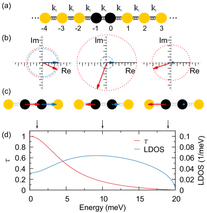
Figure 1: (a) Sketch of the 1D junction. Two semi-infinite leads with nearest-neighbor coupling constants $k_{\mathrm{l}}$ are connected at sites $-1$ and $0$ with the coupling constant $k_{\mathrm{c}}$. The region $(-\infty,-2]$ is considered as the L part, the region $[-1,0]$ as the C part and $[1,\infty)$ as the R part. (b) Transmission eigenchannel $\tilde{\bm{Q}}_{1}(E,t=0)$ for the 1D chain represented in the complex plane for energies of $E=1$ meV, 10 meV, and 19 meV. The red arrow shows the complex number $\tilde{Q}_{1,-1}(E,t=0)$ for the atom $-1$, the blue one $\tilde{Q}_{1,0}(E,t=0)$ for atom $0$. (c) The same as in panel (b), but now we display only the real part of the solution $\mathrm{Re}\tilde{\bm{Q}}_{1}(E,t=0)$. (d) The corresponding transmission eigenvalue $\tau_{1}(E)$ as a function of energy together with the LDOS of one of the atoms ($-1$ or $0$) in the central part. The energies of those eigenchannels, which are studied in panels (b) and (c), are indicated with arrows. For panels (b)–(d), we assumed spring constants of $k_{\mathrm{l}}=100$ meV² and $k_{\mathrm{c}}=20$ meV².

The Green’s function of the central part $D_{\mathrm{CC}}^{\mathrm{r}}(E)$ can be obtained from Eq. (20) using

$$K_{\mathrm{CC}}=\begin{pmatrix}k_{\mathrm{c}}+k_{\mathrm{l}}&-k_{\mathrm{c}}\\ -k_{\mathrm{c}}&k_{\mathrm{c}}+k_{\mathrm{l}}\end{pmatrix}$$ (35)

together with the self-energies

$$\Pi_{\mathrm{L}}^{\mathrm{r}}(E)=f(E)\begin{pmatrix}1&0\\ 0&0\end{pmatrix},~{}~{}\Pi_{\mathrm{R}}^{\mathrm{r}}(E)=f(E)\begin{pmatrix}0&0\\ 0&1\end{pmatrix},$$ (36)

where $f(E)=(E^{2}-2k_{\mathrm{l}}-E\sqrt{E^{2}-4k_{\mathrm{l}}})/2$. Thus, the corresponding linewidth-broadening matrices can be written as

$$\Lambda_{\mathrm{L}}(E)=g(E)\begin{pmatrix}1&0\\ 0&0\end{pmatrix},~{}~{}\Lambda_{\mathrm{R}}(E)=g(E)\begin{pmatrix}0&0\\ 0&1\end{pmatrix},$$ (37)

with

$$g(E)=\begin{cases}E\sqrt{4k_{\mathrm{l}}-E^{2}}&\mbox{if}~{}E^{2}<4k_{\mathrm{l}},\\ 0&\mbox{if}~{}E^{2}\geq 4k_{\mathrm{l}}.\end{cases}$$ (38)

From these expressions, the spectral function $A_{\mathrm{C}}^{\mathrm{L}}(E)$ in Eqs. (22) and (28) is computed. For $E^{2}<4k_{\mathrm{l}}$, the eigenvalues of this matrix are given by

$$\lambda_{1}(E)=\frac{\sqrt{4k_{\mathrm{l}}-E^{2}}[2k_{\mathrm{c}}^{2}+E^{2}(k_{\mathrm{l}}-k_{\mathrm{c}})]}{k_{\mathrm{l}}E[4k_{\mathrm{c}}^{2}+E^{2}(k_{\mathrm{l}}-2k_{\mathrm{c}})]},~{}~{}\lambda_{2}(E)=0$$ (39)

with the corresponding eigenvectors

$$\tilde{\bm{\chi}}_{1}(E) = \begin{pmatrix}\frac{-E^{2}+2k_{\mathrm{c}}-\mathrm{i}E\sqrt{4k_{\mathrm{l}}-E^{2}}}{\sqrt{8k_{\mathrm{c}}^{2}+4E^{2}\left(k_{\mathrm{l}}-k_{\mathrm{c}}\right)}}\\ \frac{k_{\mathrm{c}}}{\sqrt{2k_{\mathrm{c}}^{2}+E^{2}\left(k_{\mathrm{l}}-k_{\mathrm{c}}\right)}}\end{pmatrix},$$

$$\tilde{\bm{\chi}}_{2}(E) = \begin{pmatrix}\frac{k_{c}(E^{2}-2k_{c}+iE\sqrt{4k_{l}-E^{2}})}{2\sqrt{(k_{c}^{2}+E^{2}(k_{l}-k_{c}))(2k_{c}^{2}+E^{2}(k_{l}-k_{c}))}}\\ \frac{\sqrt{k_{c}^{2}+E^{2}(k_{l}-k_{c})}}{\sqrt{2k_{c}^{2}+E^{2}(k_{l}-k_{c})}}\end{pmatrix},$$ (40)

which are orthonormal, i.e., $\tilde{\bm{\chi}}_{m}^{\dagger}(E)\tilde{\bm{\chi}}_{n}(E)=\delta_{mn}$. From the $\tilde{\bm{\chi}}_{m}(E)$ we obtain the C projections of left-incoming scattering states $\tilde{\bm{\xi}}_{m}(E)$ by multiplying with $\sqrt{E\lambda_{m}(E)/\pi}$ [see the discussion of Eq. (28)]. Constructing $\tilde{U}(E)=\left(\tilde{\bm{\xi}}_{1}(E),\tilde{\bm{\xi}}_{2}(E)\right)$, we determine $\tau^{(1)}(E)$ via Eq. (29). Diagonalizing the resulting transmission probability matrix [see Eq. (30)], we obtain the transmission eigenvalues

$$\tau_{1}(E)=\frac{k_{\mathrm{c}}^{2}(4k_{\mathrm{l}}-E^{2})}{k_{\mathrm{l}}[4k_{\mathrm{c}}^{2}+E^{2}(k_{\mathrm{l}}-2k_{\mathrm{c}})]},~{}~{}\tau_{2}(E)=0$$ (41)

and eigenvectors

$$\bm{c}_{1}(E)=\begin{pmatrix}1\\ 0\end{pmatrix},~{}~{}\bm{c}_{2}(E)=\begin{pmatrix}0\\ 1\end{pmatrix}.$$ (42)

These coefficients determine the eigenchannels $\tilde{\bm{\Psi}}_{\mu}(E)$ via Eq. (31). The time-dependent eigenchannel displacements can now be computed through Eqs. (33) and (34) by transforming the eigenchannels to the eigenchannel displacement vectors and by multiplying with a time-dependent phase factor.

Since we assume that the masses of all atoms $m_{i}=m$ are identical in the 1D chain, eigenchannels and eigenchannel displacements are proportional $\tilde{\bm{Q}}_{\mu}(E)=s(E)\tilde{\bm{\Psi}}_{\mu}(E)/\sqrt{m}$ to each other. We therefore define $\tilde{\bm{\Psi}}_{\mu}(E,t)=\sqrt{m}\tilde{\bm{Q}}_{\mu}(t,E)/s(E)$ and use both quantities interchangeably. Choosing the global phase factor of the eigenchannel such that the component of the atom $0$ is real and positive at $t=0$, the time-dependent eigenchannels read

$$\tilde{\bm{\Psi}}_{1}(t,E)=\sqrt{\frac{\sqrt{4k_{\mathrm{l}}-E^{2}}k_{\mathrm{c}}^{2}}{\pi k_{\mathrm{l}}\left(E^{2}(k_{\mathrm{l}}-2k_{\mathrm{c}})+4k_{\mathrm{c}}^{2}\right)}}\begin{pmatrix}\frac{-E^{2}+2k_{\mathrm{c}}-\mathrm{i}E\sqrt{4k_{\mathrm{l}}-E^{2}}}{2k_{\mathrm{c}}}\\ 1\end{pmatrix}e^{-\mathrm{i}Et/\hbar},~{}~{}\tilde{\bm{\Psi}}_{2}(t,E)=0.$$ (43)

Let us discuss several points at this stage. We note that there is only a single eigenchannel with nonvanishing transmission. This is due to the fact that in our 1D model there is only nearest-neighbor coupling. Displacements, which we assume to be along the chain direction, thus need to spread sequentially from atom to atom. The leads provide a cutoff energy of $E_{\mathrm{c}}=2\sqrt{k_{\mathrm{l}}}$, above which no propagating states exist. If $0\leq k_{\mathrm{c}}\leq k_{\mathrm{l}}$ the whole junction shows no bound states, while they arise if $k_{\mathrm{c}}>k_{\mathrm{l}}\geq 0$. Due to the particular left-right symmetry of our problem, the following relations hold for $k_{\mathrm{c}}\leq k_{\mathrm{l}}$: $\rho_{ii}(E)=E[A_{ii}^{\mathrm{L}}(E)+A_{ii}^{\mathrm{R}}(E)]/\pi=E\mathrm{Tr}[A_{\mathrm{C}}^{\mathrm{L}}(E)]/\pi=E\lambda_{1}(E)/\pi=|\tilde{\bm{\Psi}}_{1}(E)|^{2}$ with $i=-1,0$. The expressions imply that the square of the norm of the transmission eigenchannel $1$ follows the LDOS of one of the atoms in the C part. Integration yields $\int_{0}^{E_{\mathrm{c}}}\mathrm{d}E\rho_{ii}(E)=\int_{0}^{E_{\mathrm{c}}}\mathrm{d}E|\tilde{\bm{\Psi}}_{1}(E)|^{2}=1$, which is consistent with the normalization condition in Eq. (II.1), since there are no bound states present. For the case $k_{\mathrm{c}}>k_{\mathrm{l}}$, we get $\int_{0}^{E_{\mathrm{c}}}\mathrm{d}E|\tilde{\bm{\Psi}}_{1}(E)|^{2}<1$, and bound-state contributions need to be taken into account in the C part to fulfill the normalization condition in Eq. (II.1).

If we now consider the perfect chain with $k_{\mathrm{c}}=k_{\mathrm{l}}$, the previous results reduce to

$$\tau_{1}(E)=1,~{}~{}\tau_{2}(E)=0$$ (44)

with

$$\tilde{\bm{\Psi}}_{1}(t,E)=\frac{1}{\sqrt{\pi\sqrt{4k_{\mathrm{l}}-E^{2}}}}\begin{pmatrix}u_{-1}(t,E)\\ u_{0}(t,E)\end{pmatrix},~{}~{}\tilde{\bm{\Psi}}_{2}(t,E)=0,$$ (45)

where $u_{n}(t,E)=\exp[\mathrm{i}k(E)nd-\mathrm{i}Et/\hbar]$. The $u_{n}(t,E)$ appear as solutions for the equation of motion of atoms arranged in an infinite chain and coupled by the same nearest-neighbor spring constants Ashcroft and Mermin (1976). Here, we have introduced the wavevector $k(E)=(2/d)\sin^{-1}(E/E_{\mathrm{c}})$ and neighboring atoms are assumed to be separated by the distance $d$. Note that the interatomic distance $d$ is not relevant for our transport problem, which is entirely determined by the force constant matrix $K$ [see Eqs. (10) and (11)], where force constants will of course be functions of interatomic distances in realistic systems. As discussed in the previous paragraph, we find that $\rho_{ii}(E)=|\tilde{\bm{\Psi}}_{1}(E)|^{2}=2/(\pi\sqrt{4k_{\mathrm{l}}-E^{2}})$ with $\int_{0}^{E_{\mathrm{c}}}\mathrm{d}E\rho_{ii}(E)=1$.

We want to use now the analytical expressions to examine different representations of the transmission eigenchannel displacements. For this purpose we choose the global scaling factor $s/\sqrt{m}$ in Eq. (33) to be real, energy-independent and of units J^1/2m/kg^1/2. In Fig. 1(b)–(d) we study the transmission, LDOS and eigenchannel displacements for the 1D chain with $k_{\mathrm{l}}=100$ meV² and $k_{\mathrm{c}}=20$ meV², i.e., in the situation where there are only propagating states in the junction system. The transmission $\tau(E)$ in Fig. 1(d) shows a monotonically decreasing behavior with increasing energy and vanishes above the cutoff energy of $E_{\mathrm{c}}=20$ meV. At the same time, we plot the LDOS $\rho_{ii}(E)$ of the atom $i=-1,0$ in the central part, which starts from a finite value at $E=0$, increases to a maximum around $9$ meV and drops to zero beyond $E_{\mathrm{c}}$. The transmission eigenchannel displacements $\tilde{\bm{Q}}_{1}(t=0,E)$ are shown in Fig. 1(b) for the energies $E=1$ meV, 10 meV, and 19 meV, indicated by arrows in Fig. 1(d). The two complex components are indicated by two arrows in the complex plane. Notice that while the norm of the eigenvector $\tilde{\bm{Q}}_{1}(t,E)$ is proportional to $\sqrt{\rho_{ii}(E)}$ for the energy-independent $s$ chosen here, the relative magnitude at the atom $i=0$ as compared to the atom $i=-1$, i.e., $|\tilde{Q}_{1,0}(t,E)|/|\tilde{Q}_{1,-1}(t,E)|$, decreases with increasing energy because a larger portion of the left-incoming wave gets reflected at the constriction. We also note that the phase difference $\theta_{0,1}(E)-\theta_{-1,1}(E)$ [see Eq. (33)] between the two components increases from $0$ at $E=0$ to $\pi$ at $E=20$ meV. With increasing time the arrows precess around the origin at a constant angular velocity of $\omega=E/\hbar$, spanning the circle indicated by the dashed lines in the plot. Since the two atoms typically do not swing in phase, the real parts of $\tilde{Q}_{1,-1}(t,E)$ and $\tilde{Q}_{1,0}(t,E)$ take maximum amplitudes at different times.

In Fig. 1(c) we present another way to visualize the eigenchannel displacements by simply plotting $\mathrm{Re}\tilde{Q}_{1,-1}(t,E)$ and $\mathrm{Re}\tilde{Q}_{1,0}(t,E)$ at $t=0$ as arrows attached to the respective atoms. This is actually the representation that we will use in all the figures shown in the rest of the paper. Notice that due to our choice of the global phase factor, we get $\theta_{0,1}(E)=0$ and $\mathrm{Re}\tilde{Q}_{1,0}(t=0,E)$ is hence maximal at $t=0$. In contrast $\mathrm{Re}\tilde{Q}_{1,-1}(t,E)$ depends both on the absolute value $|\tilde{Q}_{1,-1}(E)|$ and the phase $\theta_{-1,1}(E)$, as it is visible from Fig. 1(b). Despite the large $|\tilde{Q}_{1,-1}(E)|$ at $E=10$ meV, $\mathrm{Re}\tilde{Q}_{1,-1}(t,E)$ is rather small, because $\theta_{-1,1}(E)\approx-0.6\pi$. In spite of such shortcomings, one gets an impression of the nature of the atomic motions involved in the eigenchannel. Indeed, we observe that the eigenchannel displacements at low energy $E=1$ meV resemble a translational mode of the two atoms, while they are basically vibrating against each other at $19$ meV, as it is clear from the evolution of the phase difference $\theta_{0,1}(E)-\theta_{-1,1}(E)$ with energy, discussed in the previous paragraph. Videos could be used to examine the full time-dependent dynamics of $\mathrm{Re}\tilde{\bm{Q}}_{1}(t,E)$, but we refrain from this here, since the simple 1D case is well characterized with the help of Fig. 1(b).

III.2 Ab initio results

After illustrating the method with the simple 1D model, we apply it now to realistic systems. In these systems, we determine the force constant matrix for a particular junction geometry with the help of density functional theory (DFT) and describe the coherent phonon transport within the NEGF formalism explained in Sec. II. In particular, we will present different examples of the analysis of the phonon eigenchannels in nanoscale systems that include a gold single-atom contact Klöckner et al. (2017a) and several single-molecule junctions made of gold electrodes that are bridged by an alkane chain Klöckner et al. (2016), a C₆₀ molecule Klöckner et al. (2017b), and a benzene ring with a bromine substituent Klöckner et al. (2017c), where destructive interference effects show up in the latter case. Let us stress that we have already studied in detail the phononic thermal conductance in these systems in the references cited above. Here, we shall focus on the new insight provided by the analysis of the eigenchannels, and we refer the reader to those publications for the technical details on the calculations of the transmission functions.

In our junctions with gold electrodes, the Debye energy of the metal of around 20 meV represents the cutoff energy for the propagating states of the scattering problem. Because gas-phase molecules typically show vibrations with energies much above $E_{\mathrm{c}}$, this leads to bound states in the molecular junctions. They need to be considered for a proper normalization of the eigenchannels $\tilde{\bm{\Psi}}_{\mu}(E)$ in Eq. (31).

We visualize eigenchannels in all the figures below in terms of the static picture of the real part of the eigenchannel displacements at $t=0$, i.e., $\mathrm{Re}\tilde{\bm{Q}}_{\mu}(t=0,E)=\mathrm{Re}\tilde{\bm{Q}}_{\mu}(E)$ [see Eqs. (33) and (34)], but we illustrate the real part of the full time-dependent solutions $\mathrm{Re}\tilde{\bm{Q}}_{\mu}(t,E)$ in the form of movies online SM . In contrast to the 1D model, the masses of the atoms $m_{i}$ are different in the hetero-atomic molecular junctions. This leads to the fact that the eigenchannel displacements $\tilde{\bm{Q}}_{\mu}(E)$ are no longer proportional to the eigenchannels $\tilde{\bm{\Psi}}_{\mu}(E)$. Below, we will adjust the real-valued scaling factor $s(E)$ of Eq. (33) for an optimized visualization of eigenchannel displacements at each energy $E$. In this way, the vectors $\mathrm{Re}\tilde{\bm{Q}}_{\mu}(E)$ at different energies should only be compared on qualitative grounds, while they are fully comparable at a certain fixed energy. Since it should be obvious in which situation we mean the genuine eigenchannels $\tilde{\bm{\Psi}}_{\mu}(E)$ as compared to the eigenchannel displacements $\tilde{\bm{Q}}_{\mu}(E)$, we do not clearly distinguish them anymore and often simply refer to both as “eigenchannels” in the following. For convenience we will henceforth furthermore omit all energy arguments.

III.2.1 Gold dimer contact

The heat conductance of gold atomic contacts has been measured recently Cui et al. (2017); Mosso et al. (2017), and we have performed a detailed theoretical analysis of the thermal transport due to both electrons and phonons in these systems Cui et al. (2017); Klöckner et al. (2017a). We focus here on a gold contact that is one-atom thick and features a dimer in the narrowest part. The geometry, which is shown in Fig. 2, describes junctions with an electrical conductance of the order of the electrical conductance quantum $G_{0}=2e^{2}/h$. In Fig. 2(a)–(c) we display the energy-dependent phonon transmission together with eigenchannel representations for two different energies, as indicated by arrows in the transmission plot.

In Fig. 2(a) we show the three eigenchannels with the highest transmission for an energy of $1.5$ meV. As one can see, the first two channels correspond to modes with mainly transverse character with respect to the transport direction, whose polarizations are rather perpendicular to each other. For the first channel, with a nearly perfect transmission $\tau_{1}\approx 1$, the atomic displacements are almost symmetric on both sides of the junction. In contrast, for the second channel, with a transmission $\tau_{2}<1$, a reduced amplitude is seen on the right part as compared to the left one. This illustrates that the wave coming in from the left is mostly reflected at the central part of the junction. The third channel shows a clearly longitudinal character, and the amplitudes of atomic motion decay even more rapidly from left to right because of the low transmission probability $\tau_{3}$. Due to the small energy ($E=1.5$ meV) chosen in this example, the wavelength of atomic motion spans the central part of the junction.

To explore the behavior of the eigenchannels at shorter phonon wavelengths, we show in Fig. 2(b) the three most transmissive eigenchannels for an energy of $10.5$ meV. We find that the first mode is of a pronounced longitudinal character at the dimer in the center of the junction, and we see that the dimer atoms often move with opposite velocities, i.e., the out-of-phase character is strongly enhanced as compared to the previous in-phase motion at $E=1.5$ meV. Let us mention that, as discussed for the 1D model, due to the smaller wavelength of the vibrational modes at $E=10.5$ meV, the displacements at $t=0$ are not maximal for all of the atoms, but still one can get an impression of the nature of the mode. For the other two channels at the energy of $E=10.5$ meV the amplitudes on the right junction side are, as expected, substantially reduced due to the smaller transmission values $\tau_{2}$ and $\tau_{3}$. While the third eigenchannel exhibits predominantly a longitudinal character on the dimer atoms, no clear type can be assigned to the second eigenchannel.

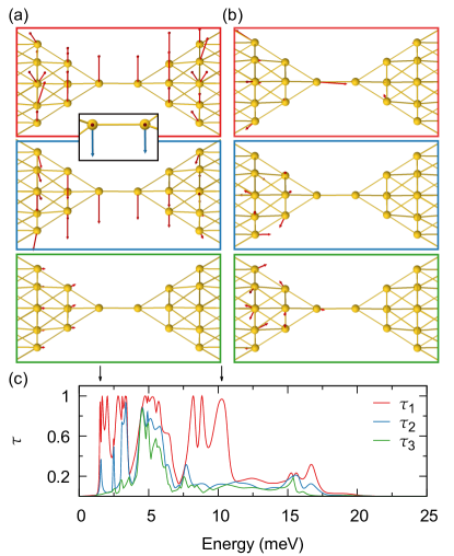
Figure 2: (a) Transmission eigenchannels for a gold dimer contact at an energy of $1.5$ meV. We show the three eigenchannels with the highest transmissions, which are equal to $\tau_{1}=0.943$, $\tau_{2}=0.238$ and $\tau_{3}=0.002$. To better visualize the perpendicular polarizations of eigenchannels 1 and 2, we have inserted an inset between these two channels. It shows both $\mathrm{Re}\tilde{\bm{Q}}_{1}(E)$ and $\mathrm{Re}\tilde{\bm{Q}}_{2}(E)$ on the dimer atoms. Red are the displacements for eigenchannel 1, blue for eigenchannel 2, and the geometry has been rotated such that the displacement vectors of channel 1 point out of plane. (b) The same as in panel (a), but for an energy of $10.5$ meV. The channel transmissions are $\tau_{1}=0.968$, $\tau_{2}=0.122$ and $\tau_{3}=0.098$. (c) The three highest transmission coefficients as a function of energy for the gold atomic contact shown in panels (a) and (b). The energies of the eigenchannels considered in these two panels are indicated by arrows, and colored frames around the channel representations serve to identify the corresponding transmission values in panel (c).

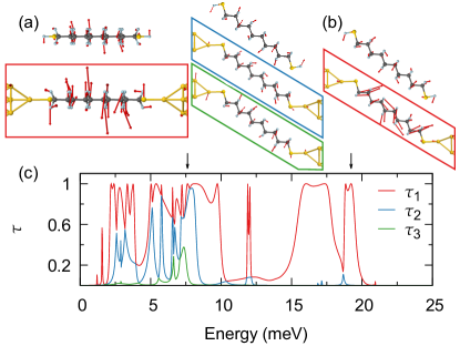
Figure 3: (a) Transmission eigenchannels for an Au-decane-dithiol-Au junction at an energy of $7.61$ meV. We show the three eigenchannels with the highest transmissions of $\tau_{1}=1.00$, $\tau_{2}=0.84$ and $\tau_{3}=0.13$ as well as two vibrational modes of the free molecule at energies of $6.4$ meV and $9.8$ meV. (b) The most transmissive eigenchannel at an energy of $19.23$ meV and a vibrational mode of the free molecule at energy $18.76$ meV. (c) Three highest transmission eigenvalues as a function of energy for the Au-decane-dithiol-Au junction. The energies of the eigenchannels shown in panels (a) and (b) are indicated with arrows. In these two panels the angle of view differs for modes with out-of-plane as compared to in-plane character.

III.2.2 Alkane contact

The phonon transport in molecular junctions based on alkane chains has been studied by several theoretical groups employing different methods Segal et al. (2003); Luo and Lloyd (2010); Duda et al. (2011); Sadeghi et al. (2015), and it has also been explored experimentally in the context of many-molecule junctions Wang et al. (2006b, 2007b); Losego et al. (2012); Meier et al. (2014); Majumdar et al. (2015). In Ref. Klöckner et al. (2016) we have studied, in particular, the length dependence of the phononic thermal conductance in single-molecule junctions based on alkane chains. Here we focus on the analysis of a single-molecule junction containing a dithiolated decane (i.e., an alkane chain with 10 CH₂ segments) coupled to gold leads. In Fig. 3(a)–(c) we display the energy-dependent transmission together with eigenchannel representations at the two different energies, indicated by arrows in the transmission plot. The eigenchannels are furthermore compared to normal modes of the isolated molecule.

In Fig. 3(a) we show the eigenchannels with the three highest transmission coefficients at the energy $E=7.61$ meV. In addition, we also show two vibrational modes of the free molecule with energies of $6.4$ meV and $9.8$ meV. Compared to the axis through the two terminal sulfur atoms, these modes can be described as predominantly transversal, but they can also be classified as out-of-plane and in-plane modes, respectively, if we consider the plane spanned by the molecular backbone of sulfur and carbon atoms. Based on the $t=0$ snapshot, the first eigenchannel shows some similarities with the first mode of the free molecule at $6.4$ meV, both modes having a clear transversal, out-of-plane character. The third eigenchannel can be related to the second mode of the free molecule at $9.8$ meV, which exhibits again a transversal in-plane character. The relation of the second transmission eigenchannel of in-plane type to a mode of the free molecule is, however, not so obvious. Let us mention that we change the perspective for all modes and eigenchannels with in-plane character as compared to those with out-of-plane type to better visualize the atomic motions involved.

Further insight into the nature of the eigenchannels can be gained by looking at the full time-dependent solutions SM . In the movies available in Ref. SM one can see that the first eigenchannel exhibits the transversal, out-of-plane character that is already apparent in the static representation of Fig. 3(a). For the second and third eigenchannel, the movies reveal similar in-plane atomic motions inside the molecule, but when compared to the sulfur-sulfur axis or those between the two Au tip atoms, they also reveal a partially longitudinal character of the second eigenchannel.

This example shows that an unambiguous identification of the eigenchannels with the modes of the free molecule is not always possible. This is also evident when considering the phase factors related to traveling waves [see the terms $u_{n}(t,E)$ discussed in subsection III.1], which do not appear in an isolated molecule. Nevertheless, a qualitative relation of the eigenchannels to free modes can sometimes still be seen.

In Fig. 3(b) we display the most transmissive eigenchannel at an energy of $19.23$ meV along with a vibrational mode of the free molecule with energy $18.76$ meV that exhibits a very similar character. The eigenchannel in this case is mainly of longitudinal, in-plane type, like the free-molecule mode. Note the shorter wavelength of the propagating wave at the higher energy in Fig. 3(b) as compared to Fig. 3(a) in the static representation of the eigenchannel.

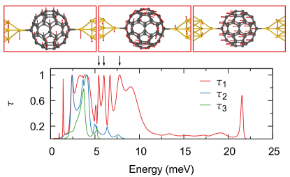
Figure 4: The three largest transmission coefficients for a Au-C₆₀-Au junction as a function of energy. The most transmissive eigenchannels at energies of $5.4$ meV, $6.0$ meV and $7.8$ meV, as indicated by arrows in the transmission plot, are shown in the upper part of the figure.

III.2.3 C₆₀ contact

Let us now discuss the case of an Au-C₆₀-Au junction, see Fig. 4, which we have analyzed in Ref. Klöckner et al. (2017b) in the context of the thermoelectric figure of merit of fullerene-based junctions. This is a very interesting case because all the vibrational modes of the free molecule have an energy that is higher than the Au Debye energy. So one may wonder, how phonon transport can occur in this junction and why it is not completely suppressed. This can be nicely answered with the help of the transmission eigenchannels.

For this purpose, we present in Fig. 4 the most transmissive eigenchannels at energies of $5.4$ meV, $6.0$ meV, and $7.8$ meV above a plot of the energy-dependent transmission. As one can see, all the eigenchannels correspond to a hybridization of the vibrations of the gold atoms with the center-of-mass motion of the C₆₀ molecule. The eigenchannel at $5.4$ meV possesses a transversal character, where the molecule moves up and down as a whole, and it also involves transversal motions of the gold atoms in the electrode tips. The eigenchannel at $6.0$ meV involves a rotation of the molecule that is again coupled to transversal vibrations of the gold atoms. Finally, the eigenchannel at $7.8$ meV involves a longitudinal center-of-mass motion of the C₆₀ that is coupled to a predominantly longitudinal movement of the Au tip atoms. Let us point out that in the movies of the eigenchannels, a small deformation of the C₆₀ molecule can also be seen in all three examples in addition to the main center-of-mass motion highlighted by the static pictures SM .

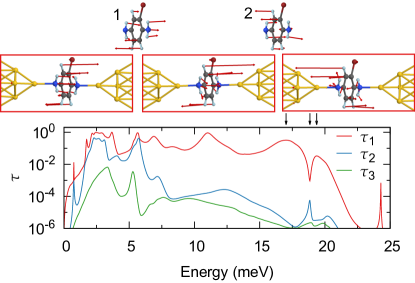
Figure 5: The three highest eigenchannel transmissions as a function of energy for a Au-2-bromo-1,4-diaminobenzene-Au junction. Above the graph, one can see the eigenchannels with the highest transmission for the three different energies of $17.03$ meV, $18.85$ meV, and $19.37$ meV. The energies are selected by peaks of $\tau_{1}$ in the transmission plot and are indicated by corresponding arrows. Above the eigenchannels we show the vibrational modes of the free molecule that are responsible for the destructive interference.

III.2.4 Brominated benzene-diamine contact

Another important example, in which the eigenchannel concept provides a better understanding, is the case when destructive interference effects occur in the phonon transport. We have shown in Ref. Klöckner et al. (2017c) that the introduction of substituents in benzene molecules can lead to the appearance of destructive interferences in corresponding single-molecule junctions based on Au electrodes, despite their low Debye energy. The interference effects are reflected in the appearance of antiresonances in the phonon transmission.

In Fig. 5 we show the energy dependence of the three largest eigenchannel transmissions of an Au-2-bromo-1,4-diaminobenzene-Au junction studied in Ref. Klöckner et al. (2017c), in which an antiresonance appears at around $19$ meV. We have attributed this antiresonance to the interference of the two out-of-plane modes of the free molecule that lie close in energy at $15.61$ meV and $20.07$ meV and that are shown in the upper part of Fig. 5. In that figure we also display the most transmissive eigenchannel for three different energies, which dominates the phonon transport. As can be seen, this eigenchannel exhibits indeed a character that closely resembles those of the two vibrational modes of the free molecule at similar energies. Additionally, in the static picture of the eigenchannel shown in Fig. 5, one can see a jump of $\pi$ in the phase of molecular motion as compared to the Au reference atoms, which is reflected by the fact that the arrows on the molecule point in opposite directions at energies above and below the antiresonance. This jump in the phase is a well-known phenomenon that accompanies destructive interference in the electronic transport Solomon et al. (2010) and, in general, in the Fano model Joe et al. (2006).

Our example illustrates how the eigenchannel concept helps to identify the molecular origin of destructive quantum interference. This is particularly useful in cases in which is not easy to figure out the vibrational modes responsible for the interference phenomenon, because of the presence of many other modes in that energy region or because the energies of the vibrations of the free molecule are strongly renormalized by the hybridization with the metallic leads when the molecule is connected to the electrodes.

IV Conclusions

In this work, and in analogy with what is done in electronic transport, we have presented a method to obtain the transmission eigenchannels from NEGF-based calculations of the coherent phonon transport. In particular, we have shown that this method can be combined with ab initio simulations to provide an insight into phonon transport that cannot simply be obtained from the analysis of the transmission probabilities. We have illustrated this approach with the analysis of the phonon eigenchannels in realistic atomic-scale junctions, including single-atom and single-molecule junctions. Moreover, we have discussed different ways to visualize these eigenchannels by means of static and time-dependent representations. We believe that the procedure presented in this work will become a valuable tool for the analysis of coherent phonon transport in a great variety of nanoscale systems and devices.

V Acknowledgments

J.C.K. and F.P. thank M. Bürkle for stimulating discussions in the initial phase of this work. In addition, both gratefully acknowledge funding from the Carl Zeiss foundation, the Junior Professorship Program of the Ministry of Science, Research and the Arts of the state of Baden Württemberg, and the Collaborative Research Center (SFB) 767 of the German Research Foundation (DFG). J.C.C. thanks the Spanish Ministry of Economy and Competitiveness (Contract No. FIS2017-84057-P) for financial support as well as the DFG and SFB 767 for sponsoring his stay at the University of Konstanz as Mercator Fellow. An important part of the numerical modeling was carried out on the computational resources of the bwHPC program, namely the bwUniCluster and the JUSTUS HPC facility.

References

- Cahill et al. (2003) D. G. Cahill, W. K. Ford, K. E. Goodson, G. D. Mahan, A. Majumdar, H. J. Maris, R. Merlin, and S. R. Phillpot, “Nanoscale thermal transport,” J. Appl. Phys. 93, 793 (2003).
- Pop (2010) E. Pop, “Energy dissipation and transport in nanoscale devices,” Nano Res. 3, 147 (2010).
- Luo and Chen (2013) T. Luo and G. Chen, “Nanoscale heat transfer - from computation to experiment,” Phys. Chem. Chem. Phys. 15, 3389 (2013).
- Cahill et al. (2014) D. G. Cahill, P. V. Braun, G. Chen, D. R. Clarke, S. Fan, K. E. Goodson, P. Keblinski, W. P. King, G. D. Mahan, A. Majumdar, H. J. Maris, S. R. Phillpot, E. Pop, and L. Shi, “Nanoscale thermal transport. II. 2003–2012,” Appl. Phys. Rev. 1, 011305 (2014).
- Cui et al. (2017) L. Cui, W. Jeong, S. Hur, M. Matt, J. C. Klöckner, F. Pauly, P. Nielaba, J. C. Cuevas, E. Meyhofer, and P. Reddy, “Quantized thermal transport in single-atom junctions,” Science 355, 1192 (2017).
- Mosso et al. (2017) N. Mosso, U. Drechsler, F. Menges, P. Nirmalraj, S. Karg, H. Riel, and B. Gotsmann, “Heat transport through atomic contacts,” Nat. Nanotech. 12, 430 (2017).
- Minnich (2015) A. J. Minnich, “Advances in the measurement and computation of thermal phonon transport properties,” J. Phys.: Condens. Matter 27, 053202 (2015).
- Cuevas and Scheer (2017) J. C. Cuevas and E. Scheer, Molecular Electronics: An Introduction to Theory and Experiment, 2nd ed. (World Scientific, Singapore, 2017).
- Segal and Agarwalla (2016) D. Segal and B. K. Agarwalla, “Vibrational heat transport in molecular junctions,” Annu. Rev. Phys. Chem. 67, 185 (2016).
- Fagas et al. (1999) G. Fagas, A. G. Kozorezov, C. J. Lambert, J. K. Wigmore, A. Peacock, A. Poelaert, and R. den Hartog, “Lattice dynamics of a disordered solid-solid interface,” Phys. Rev. B 60, 6459 (1999).
- Zhao and Freund (2005) H. Zhao and J. B. Freund, “Lattice-dynamical calculation of phonon scattering at ideal Si-Ge interfaces,” J. Appl. Phys. 97, 024903 (2005).
- Wang and Wang (2006) J. Wang and J.-S. Wang, “Mode-dependent energy transmission across nanotube junctions calculated with a lattice dynamics approach,” Phys. Rev. B 74, 054303 (2006).
- Duchemin and Donadio (2011) I. Duchemin and D. Donadio, “Atomistic calculation of the thermal conductance of large scale bulk-nanowire junctions,” Phys. Rev. B 84, 115423 (2011).
- Zhang et al. (2011) L. Zhang, P. Keblinski, J.-S. Wang, and B. Li, “Interfacial thermal transport in atomic junctions,” Phys. Rev. B 83, 064303 (2011).
- Tanaka et al. (2005) Y. Tanaka, F. Yoshida, and S. Tamura, “Lattice thermal conductance in nanowires at low temperatures: Breakdown and recovery of quantization,” Phys. Rev. B 71, 205308 (2005).
- Antonyuk et al. (2005) V. B. Antonyuk, M. Larsson, A. G. Mal’shukov, and K. A. Chao, “Phonon transmission in III-V semiconductor superlattices and alloys,” Semicond. Sci. Technol. 20, 347 (2005).
- Murphy and Moore (2007) P. G. Murphy and J. E. Moore, “Coherent phonon scattering effects on thermal transport in thin semiconductor nanowires,” Phys. Rev. B 76, 155313 (2007).
- Mingo and Yang (2003) N. Mingo and L. Yang, “Phonon transport in nanowires coated with an amorphous material: An atomistic Green’s function approach,” Phys. Rev. B 68, 245406 (2003).
- Mingo (2006) N. Mingo, “Anharmonic phonon flow through molecular-sized junctions,” Phys. Rev. B 74, 125402 (2006).
- Asai (2008) Y. Asai, “Nonequilibrium phonon effects on transport properties through atomic and molecular bridge junctions,” Phys. Rev. B 78, 045434 (2008).
- Markussen (2013) T. Markussen, “Phonon interference effects in molecular junctions,” J. Chem. Phys. 139, 244101 (2013).
- Sadeghi et al. (2015) H. Sadeghi, S. Sangtarash, and C. J. Lambert, “Oligoyne molecular junctions for efficient room temperature thermoelectric power generation,” Nano Lett. 15, 7467 (2015).
- Bürkle et al. (2015) M. Bürkle, T. J. Hellmuth, F. Pauly, and Y. Asai, “First-principles calculation of the thermoelectric figure of merit for [2,2]paracyclophane-based single-molecule junctions,” Phys. Rev. B 91, 165419 (2015).
- Li et al. (2015) Q. Li, I. Duchemin, S. Xiong, G. C. Solomon, and D. Donadio, “Mechanical tuning of thermal transport in a molecular junction,” J. Phys. Chem. C 119, 24636 (2015).
- Li et al. (2017) Q. Li, M. Strange, I. Duchemin, D. Donadio, and G. C. Solomon, “A strategy to suppress phonon transport in molecular junctions using -stacked systems,” J. Phys. Chem. C 121, 7175 (2017).
- Buerkle and Asai (2017) M. Buerkle and Y. Asai, “Thermal conductance of teflon and polyethylene: Insight from an atomistic, single-molecule level,” Sci. Rep. 7, 41898 (2017).
- Famili et al. (2017) M. Famili, I. Grace, H. Sadeghi, and C. J. Lambert, “Suppression of phonon transport in molecular Christmas trees,” Chem. Phys. Chem. 18, 1234 (2017).
- Wang et al. (2008) J.-S. Wang, J. Wang, and J. T. Lü, “Quantum thermal transport in nanostructures,” Eur. Phys. J. B 62, 381 (2008).
- Brandbyge et al. (1997) M. Brandbyge, M. R. Sørensen, and K. W. Jacobsen, “Conductance eigenchannels in nanocontacts,” Phys. Rev. B 56, 14956 (1997).
- Cuevas et al. (1998) J. C. Cuevas, A. Levy Yeyati, and A. Martín-Rodero, “Microscopic origin of conducting channels in metallic atomic-size contacts,” Phys. Rev. Lett. 80, 1066 (1998).
- Scheer et al. (1998) E. Scheer, N. Agraït, J. C. Cuevas, A. L. Yeyati, B. Ludoph, A. Martí要-Rodero, G. R. Bollinger, J. M. van Ruitenbeek, and C. Urbina, “The signature of chemical valence in the electrical conduction through a single-atom contact,” Nature 394, 154 (1998).
- Agraït et al. (2003) N. Agraït, A. L. Yeyati, and J. M. van Ruitenbeek, “Quantum properties of atomic-sized conductors,” Phys. Rep. 377, 81 (2003).
- Scheer et al. (1997) E. Scheer, P. Joyez, D. Esteve, C. Urbina, and M. H. Devoret, “Conduction channel transmissions of atomic-size aluminum contacts,” Phys. Rev. Lett. 78, 3535 (1997).
- Scheer et al. (2001) E. Scheer, W. Belzig, Y. Naveh, M. H. Devoret, D. Esteve, and C. Urbina, “Proximity effect and multiple Andreev reflections in gold atomic contacts,” Phys. Rev. Lett. 86, 284 (2001).
- Schirm et al. (2013) C. Schirm, M. Matt, F. Pauly, J. C. Cuevas, P. Nielaba, and E. Scheer, “A current-driven single-atom memory,” Nat. Nanotech. 8, 645 (2013).
- van den Brom and van Ruitenbeek (1999) H. E. van den Brom and J. M. van Ruitenbeek, “Quantum suppression of shot noise in atom-size metallic contacts,” Phys. Rev. Lett. 82, 1526 (1999).
- Cron et al. (2001) R. Cron, M. F. Goffman, D. Esteve, and C. Urbina, “Multiple-charge-quanta shot noise in superconducting atomic contacts,” Phys. Rev. Lett. 86, 4104 (2001).
- Djukic and van Ruitenbeek (2006) D. Djukic and J. M. van Ruitenbeek, “Shot noise measurements on a single molecule,” Nano Lett. 6, 789 (2006).
- Kiguchi et al. (2008) M. Kiguchi, O. Tal, S. Wohlthat, F. Pauly, M. Krieger, D. Djukic, J. C. Cuevas, and J. M. van Ruitenbeek, “Highly conductive molecular junctions based on direct binding of benzene to platinum electrodes,” Phys. Rev. Lett. 101, 046801 (2008).
- Vardimon et al. (2013) R. Vardimon, M. Klionsky, and O. Tal, “Experimental determination of conduction channels in atomic-scale conductors based on shot noise measurements,” Phys. Rev. B 88, 161404 (2013).
- Karimi et al. (2016) M. A. Karimi, S. G. Bahoosh, M. Herz, R. Hayakawa, F. Pauly, and E. Scheer, “Shot noise of 1,4-benzenedithiol single-molecule junctions,” Nano Lett. 16, 1803 (2016).
- Ong and Zhang (2015) Z.-Y. Ong and G. Zhang, “Efficient approach for modeling phonon transmission probability in nanoscale interfacial thermal transport,” Phys. Rev. B 91, 174302 (2015).
- Sadasivam et al. (2017) S. Sadasivam, U. V. Waghmare, and T. S. Fisher, “Phonon-eigenspectrum-based formulation of the atomistic Green’s function method,” Phys. Rev. B 96, 174302 (2017).
- Xie et al. (2011) Z.-X. Xie, K.-Q. Chen, and W. Duan, “Thermal transport by phonons in zigzag graphene nanoribbons with structural defects,” J. Phys.: Condens. Matter 23, 315302 (2011).
- Wang et al. (2011) J. Wang, L. Li, and J.-S. Wang, “Tuning thermal transport in nanotubes with topological defects,” Appl. Phys. Lett. 99, 091905 (2011).
- Ouyang et al. (2012) T. Ouyang, Y. Chen, L.-M. Liu, Y. Xie, X. Wei, and J. Zhong, “Thermal transport in graphyne nanoribbons,” Phys. Rev. B 85, 235436 (2012).
- Peng and Chen (2014) X.-F. Peng and K.-Q. Chen, “Thermal transport for flexural and in-plane phonons in graphene nanoribbons,” Carbon 77, 360 (2014).
- Paulsson and Brandbyge (2007) M. Paulsson and M. Brandbyge, “Transmission eigenchannels from nonequilibrium Green’s functions,” Phys. Rev. B 76, 115117 (2007).
- Bürkle et al. (2012) M. Bürkle, J. K. Viljas, D. Vonlanthen, A. Mishchenko, G. Schön, M. Mayor, T. Wandlowski, and F. Pauly, “Conduction mechanisms in biphenyl dithiol single-molecule junctions,” Phys. Rev. B 85, 075417 (2012).
- Farina (1973) J. E. G. Farina, Quantum theory of scattering processes (The international encyclopedia of physical chemistry and chemical physics. Topic 2: Classical and quantum mechanics, v. 4), 1st ed. (Pergamon Press, Oxford, 1973).
- Zhang et al. (2007) W. Zhang, T. S. Fisher, and N. Mingo, “The atomistic Green’s function method: An efficient simulation approach for nanoscale phonon transport,” Numer. Heat Transfer, Part B 51, 333 (2007).
- Wang et al. (2006a) J.-S. Wang, J. Wang, and N. Zeng, “Nonequilibrium Green’s function approach to mesoscopic thermal transport,” Phys. Rev. B 74, 033408 (2006a).
- Wang et al. (2007a) J.-S. Wang, N. Zeng, J. Wang, and C. K. Gan, “Nonequilibrium Green’s function method for thermal transport in junctions,” Phys. Rev. E 75, 061128 (2007a).
- Yamamoto and Watanabe (2006) T. Yamamoto and K. Watanabe, “Nonequilibrium Green’s function approach to phonon transport in defective carbon nanotubes,” Phys. Rev. Lett. 96, 255503 (2006).
- Wang et al. (2014) J.-S. Wang, B. K. Agarwalla, H. Li, and J. Thingna, “Nonequilibrium Green’s function method for quantum thermal transport,” Front. Phys. 9, 673 (2014).
- Das and Dhar (2012) S. G. Das and A. Dhar, “Landauer formula for phonon heat conduction: relation between energy transmittance and transmission coefficient,” Eur. Phys. J. B 85, 372 (2012).
- (57) See Supplemental Material at http://link.aps.org/supplemental/??? for video files showing time-dependent representations of the eigenchannels of each atomic and molecular junction.
- Ashcroft and Mermin (1976) N. W. Ashcroft and N. Mermin, Solid State Physics (Hartcourt, Orlando, 1976).
- Klöckner et al. (2017a) J. C. Klöckner, M. Matt, P. Nielaba, F. Pauly, and J. C. Cuevas, “Thermal conductance of metallic atomic-size contacts: Phonon transport and Wiedemann-Franz law,” Phys. Rev. B 96, 205405 (2017a).
- Klöckner et al. (2016) J. C. Klöckner, M. Bürkle, J. C. Cuevas, and F. Pauly, “Length dependence of the thermal conductance of alkane-based single-molecule junctions: An ab initio study,” Phys. Rev. B 94, 205425 (2016).
- Klöckner et al. (2017b) J. C. Klöckner, R. Siebler, J. C. Cuevas, and F. Pauly, “Thermal conductance and thermoelectric figure of merit of -based single-molecule junctions: Electrons, phonons, and photons,” Phys. Rev. B 95, 245404 (2017b).
- Klöckner et al. (2017c) J. C. Klöckner, J. C. Cuevas, and F. Pauly, “Tuning the thermal conductance of molecular junctions with interference effects,” Phys. Rev. B 96, 245419 (2017c).
- Segal et al. (2003) D. Segal, A. Nitzan, and P. Hänggi, “Thermal conductance through molecular wires,” J. Chem. Phys. 119, 6840 (2003).
- Luo and Lloyd (2010) T. Luo and J. R. Lloyd, “Non-equilibrium molecular dynamics study of thermal energy transport in Au-SAM-Au junctions,” Int. J. Heat Mass Transfer 53, 1 (2010).
- Duda et al. (2011) J. C. Duda, C. B. Saltonstall, P. M. Norris, and P. E. Hopkins, “Assessment and prediction of thermal transport at solid-self-assembled monolayer junctions,” J. Chem. Phys. 134, 094704 (2011).
- Wang et al. (2006b) R. Y. Wang, R. A. Segalman, and A. Majumdar, “Room temperature thermal conductance of alkanedithiol self-assembled monolayers,” Appl. Phys. Lett. 89, 173113 (2006b).
- Wang et al. (2007b) Z. Wang, J. A. Carter, A. Lagutchev, Y. K. Koh, N.-H. Seong, D. G. Cahill, and D. D. Dlott, “Ultrafast flash thermal conductance of molecular chains,” Science 317, 787 (2007b).
- Losego et al. (2012) M. D. Losego, M. E. Grady, N. R. Sottos, D. G. Cahill, and P. V. Braun, “Effects of chemical bonding on heat transport across interfaces,” Nat. Mater. 11, 502 (2012).
- Meier et al. (2014) T. Meier, F. Menges, P. Nirmalraj, H. Hölscher, H. Riel, and B. Gotsmann, “Length-dependent thermal transport along molecular chains,” Phys. Rev. Lett. 113, 060801 (2014).
- Majumdar et al. (2015) S. Majumdar, J. A. Sierra-Suarez, S. N. Schiffres, W.-L. Ong, C. F. Higgs, A. J. H. McGaughey, and J. A. Malen, “Vibrational mismatch of metal leads controls thermal conductance of self-assembled monolayer junctions,” Nano Lett. 15, 2985 (2015).
- Solomon et al. (2010) G. C. Solomon, C. Herrmann, T. Hansen, V. Mujica, and M. A. Ratner, “Exploring local currents in molecular junctions,” Nat. Chem. 2, 223 (2010).
- Joe et al. (2006) Y. S. Joe, A. M. Satanin, and C. S. Kim, “Classical analogy of Fano resonances,” Phys. Scr. 74, 259 (2006).