NEW SIZE HIERARCHIES FOR TWO WAY AUTOMATA

Abstract.

We introduce a new type of nonuniform two–way automaton that can use a different transition function for each tape square. We also enhance this model by allowing to shuffle the given input at the beginning of the computation. Then we present some hierarchy and incomparability results on the number of states for the types of deterministic, nondeterministic, and bounded-error probabilistic models. For this purpose, we provide some lower bounds for all three models based on the numbers of subfunctions and we define two witness functions.

Kamil Khadiev^1,2, Rishat Ibrahimov², and Abuzer Yakaryılmaz¹
NEW SIZE HIERARCHIES FOR TWO WAY AUTOMATA

¹Center for Quantum Computer Science, Faculty of Computing, University of Latvia Raina bulv. 19, Rīga, LV-1586, Latvia
² Kazan Federal University, Kremlevskaya Str. 18, 420008, Kazan, Russia

E-mail address: kamilhadi@gmail.com, rishat.ibrahimov@yandex.ru, abuzer@lu.lv

 

2000 Mathematical Subject Classification. 46L51, 46L53, 46E30, 46H05.

Key words and phrases. Two–way nonuniform automaton, size hierarchy, deterministic and nondeterministic models, probabilistic computation.

1. Introduction

Nonuniform models (like circuits, branching programs, uniform models using advice, etc.) have played significant roles in computational complexity, and, naturally they have also been investigated in automata theory (e.g. [7, 12, 14, 6]). The main computational resource for nonuniform automata is the number of internal states that depends on the input size. Thus we can define linear, polynomial, or exponential size automata models. In this way, for example, nonuniform models allow us to formulate the analog of “$\sf P$ versus $\sf NP$ problem” in automata theory: Sakoda and Sipser [24] conjectured that simulating a two–way nondeterministic automaton by two–way deterministic automata requires exponential number of states in the worst case. But, the best known separation is only quadratic ($O(n^{2})$) [9, 13] and the researchers have succeeded to obtain slightly better bounds only for some modified models (e.g. [21, 15, 11, 16]). Researchers also considered similar question for OBDD model that can be seen as nonuniform automata (e.g. [18], [20], [4], [2], [1], [19]).

In this paper, we present some hierarchy results for deterministic, nondeterministic, and bounded-error probabilistic nonuniform two–way automata models, which can also be seen as a “two–way” version of ordered binary decision diagrams (OBDDs) [27]. For each input length ($n$), our models can have different number of states, and, like Branching programs or the data-independent models defined by Holzer [12], the transition functions can be changed during the computation. Holzer’s model can use a different transition function for each step. We restrict this property so that the transition function is the same for the same tape positions, and so, we can have at most $n$ different transition functions. Moreover, we enhance our models by shuffling the input symbols at the beginning of the computation. We give the definitions and related complexity measures in Section 2.

In order to obtain our main results, we start with presenting some generic lower bounds (Section 3) by using the techniques given in [25] and [10]. Then, we define two witness Boolean functions in Section 3.2.1: Shuffled Address Function, denoted $\mathtt{2\mbox{-}SAF_{t}}$, which is a modification of Boolean functions given in [22] (see also [5], [8], [13], [17]), and its uniform version $\mathtt{2\mbox{-}USAF_{t}}$. Moreover, regarding these functions, we provide two deterministic algorithms. In our results, we also use the well known Equality function $\mathsf{EQ(X)}=\bigvee_{0}^{\lfloor n/2\rfloor-1}x_{i}=x_{i+\lfloor n/2\rfloor}$.

In Sections 4 and 5, we present our main results based on the size (the number of states) of models. We obtain linear size separations for deterministic models and quadratic size separations for nondeterministic and probabilistic models. Moreover, we investigate the effect of shuffling for all three types of models, and, we show that in some cases shuffling can save huge amount of states and in some other cases shuffling cannot be size efficient. We also show that the constant number of states does not increase the computational power of deterministic and nondeterministic nonuniform models without shuffling.

2. Definitions

Our alphabet is binary, $\Sigma=\{0,1\}$. We mainly use the terminologies of Branching programs: Our decision problems are solving/computing Boolean functions: The automaton solving a function accepts the inputs where the function gets the value true and rejects the inputs where the function gets the value false. For uniform models, on the other hand, our decision problems are recognizing languages: The automaton recognizing a language accepts any member and rejects any non-member.

A nonuniform head–position–dependent two–way deterministic automaton working on the inputs of length/size $n\geq 0$ (2DA_n) $D_{n}$ is a 6-tuple

$$D_{n}=(\Sigma,S,s_{1},\delta=\{\delta_{1},\ldots,\delta_{n}\},s_{a},s_{r}),$$

where (i) $S=\{s_{1},\ldots,s_{d}\}$ is the set of states ($d$ can be a function in $n$) and $s_{1},s_{a},s_{r}\in S$ ($s_{a}\neq s_{r}$) are the initial, accepting, and rejecting states, respectively; and, (ii) $\delta$ is a collection of $n$ transition functions such that $\delta_{i}:S\setminus\{s_{a},s_{r}\}\times\Sigma\rightarrow S\times\{\leftarrow,\downarrow,\rightarrow\}$ is the transition function that governs behaviour of $D_{n}$ when reading the $i$th symbol/variable of the input, where $1\leq i\leq n$. Any given input $u\in\Sigma^{n}$ is placed on a read-only tape with a single head as $u_{1}u_{2}\cdots u_{n}$ from the squares 1 to $|u|=n$, where $u_{i}\in\Sigma$ is the $i$th symbol of $u$. When $D_{n}$ is in $s\in S\setminus\{s_{a},s_{r}\}$ and reads $u_{i}\in\Sigma$ on the tape, it switches to state $s^{\prime}\in S$ and updates the head position with respect to $a\in\{\leftarrow,\downarrow,\rightarrow\}$ if $\delta_{i}(s,u_{i})\rightarrow(s^{\prime},a)$. If $a=``\leftarrow"$ ($``\rightarrow"$), the head moves one square to the left (the right), and, it stays on the same square, otherwise. The transition functions $\delta_{1}$ and $\delta_{n}$ must be defined to guarantee that the head never leaves $u$ during the computation. Moreover, the automaton enters $s_{a}$ or $s_{r}$ only on the right most symbol and then the input is accepted or rejected, respectively.

The nondeterministic counterpart of 2DA_n, denoted 2NA_n, can choose from more than one transition in each step. So, the range of each transition function is $\mathcal{P}(S\times\{\leftarrow,\downarrow,\rightarrow\})$, where $\mathcal{P}(\cdot)$ is the power set of any given set. Therefore, a 2NA_n can follow more than one computational path and the input is accepted only if one of them ends with the decision of “acceptance”. Note that some paths end without any decision since the transition function can yield the empty set for some transitions.

The probabilistic counterpart of 2DA_n, denoted 2PA_n, is a 2NA_n such that each transition is associated with a probability. Thus, 2PA_ns can be in a probability distribution over the deterministic configurations (the state and the position of head forms a configuration) during the computation. To be a well-formed machine, the total probability must be 1, i.e. the probability of outgoing transitions from a single configuration must be always 1. Thus, each input is accepted and rejected by a 2PA_n with some probabilities. An input is said to be accepted/rejected by a (bounded-error) 2PA_n if the accepting/rejecting probability by the machine is at least $1/2+\varepsilon$ for some $\varepsilon\in(0,1/2]$.

A function $f_{n}:\Sigma^{n}\rightarrow\Sigma$ is said to be computed by a 2DA_n $D_{n}$ (a 2NA_n $N_{n}$, a 2PA_n $P_{n}$) if each member of $f_{n}^{-1}(1)$ is accepted by $D_{n}$ ($N_{n}$, $P_{n}$) and each member of $f_{n}^{-1}(0)$ is rejected by $D_{n}$ ($N_{n}$, $P_{n}$).

The class $\mathsf{2DSIZE(d(n))}$ is formed by the functions $f=\{f_{0},f_{1},f_{2},\ldots\}$ such that each $f_{i}$ is computed by a 2DA_i $D_{i}$, the number of states of which is no more than $d(i)$, where $i$ is a non-negative integer. We can similarly define nondeterministic and probabilistic counterparts of this class, denoted $\mathsf{2NSIZE(d(n))}$ and $\mathsf{2PSIZE(d(n))}$ respectively.

We also introduce a generalization of our nonuniform models that can shuffle the input at the beginning of the computation with respect to a permutation. A nonuniform head–position–dependent shuffling two–way deterministic automaton working on the inputs of length/size of $n\geq 0$ (2DA${}^{\Theta}_{n}$), say $D^{\theta}_{n}$, is a 2DA_n that shuffles the symbols of input with respect to $\theta$, a permutation of $\{1,\ldots,n\}$, i.e. the $j$-th symbol of the input is placed on $\theta(j)$-th place on the tape ($1\leq j\leq n$), and then execute the 2DA_n algorithm on this new input. The nondeterministic and probabilistic models can be respectively abbreviated as 2NA${}^{\Theta}_{n}$ and 2PA${}^{\Theta}_{n}$.

The class $\mathsf{2D\Theta SIZE(d(n))}$ is formed by the functions $f=\{f_{0},f_{1},f_{2},\ldots\}$ such that each $f_{i}$ is computed by a 2DA${}^{\Theta}_{i}$ $D^{\theta}_{i}$ whose number of states is no more than $d(i)$, where $i$ is a non-negative integer and $\theta$ is a permutation of $\{1,\ldots,n\}$. The nondeterministic and probabilistic classes are respectively represented by $\mathsf{2N\Theta SIZE(d(n))}$ and $\mathsf{2P\Theta SIZE(d(n))}$.

Moreover we consider uniform versions of two-way automata, respectively 2DFA and 2NFA. We can define 2DFA in the same way as 2DA_n, but it is identical for all $n$, $|S|=const$ and $\delta_{i}=\delta$ for any $i\in\{1,\ldots,n\}$. Moreover, they can use end-markers, between which the given input is placed on the input tape. We can define 2NFA similarly. The corresponding classes of languages defined by 2DFAs and 2NFAs of size $d$ are denoted $\mathsf{2DFASIZE(d)}$ and $\mathsf{2NFASIZE(d)}$, respectively.

3. Lower bounds, Boolean functions, and algorithms

Our key complexity measure behind our results is the number of subfunctions for a given function. It can be seen as the counterpart of “the equivalence classes of a language” with respect to Myhill-Nerode Theorem [23].

Let $f$ be a Boolean function defined on $X=\{x_{1},\ldots,x_{n}\}$. We define the set of all permutations of $(1,\ldots,n)$ as $\Theta(n)$. Let $\theta\in\Theta(n)$ be a permutation. We can order the elements of $X$ with respect to $\theta$, say $(x^{\prime}_{1},\ldots,x^{\prime}_{n})$, and then we can split them into two disjoint non-empty (ordered) sets by picking an index $i\in\{1,\ldots,n-1\}$: $X_{A}=(x^{\prime}_{1},\ldots,x^{\prime}_{i})$ and $X_{B}=(x^{\prime}_{i+1},\ldots,x^{\prime}_{n})$. Let $\rho$ be a mapping $\{x^{\prime}_{1},\ldots,x^{\prime}_{i}\}\rightarrow\{0,1\}^{i}$ that assigns a value to each $x^{\prime}_{j}\in(x^{\prime}_{1},\ldots,x^{\prime}_{i})$. Then, we define function $f|_{\rho}:X_{B}\rightarrow\{0,1\}$ that returns the value of $f$ where the values of the input from $X_{A}$ are fixed by $\rho$. The function $f|_{\rho}$ is called a subfunction.

The total number of different subfunctions with respect to $\theta$ and $i$ is denoted by $N_{i}^{\theta}(f)$. Then, we focus on the maximum value by considering all possible indices:

$$N^{\theta}(f)=\max_{i\in\{1,\ldots,n-1\}}N_{i}^{\theta}(f).$$

After this, we focus on the best permutation that minimizes the number of subfunctions:

$$N(f)=\min_{\theta\in\Theta(n)}N^{\theta}(f).$$

Now, we represent the relation between the number of subfunctions for Boolean function and the number of equivalence classes of a language.

Let $L$ be a language defined on $\Sigma=\{0,1\}$. For a given non-negative integer $n$, $L_{n}$ is the language composed by all members of $L$ with length $n$, i.e. $L_{n}=L\cap\Sigma^{n}=\{w\mid w\in L,|w|=n\}$. For $r<n$, two strings $u\in\Sigma^{r}$ and $v\in\Sigma^{r}$ are said to be equivalent if for any $y\in\Sigma^{n-r}$, $uy\in L_{n}$ if and only if $vy\in L_{n}$.

We denote the number of non-equivalent strings of length $r$ as $R^{r}(L_{n})$. Then, similar to the number of subfunctions,

$$R(L_{n})=\max_{r\in\{1,\ldots,n-1\}}R^{r}(L_{n})\mbox{ and }R_{n}(L)=R(L_{n}).$$

The function $f_{n}^{L}(X)$ denotes the characteristic Boolean function for language $L_{n}$. Thus, we can say that

$$N^{id}(f_{n}^{L})=R_{n}(L).$$

for $id=(1,\dots,n)$ is natural order.

3.1. Lower bounds

First we give our lower bounds on the sizes of models in terms of $N(f)$. Note that all of lower bounds for shuffling models are valid also for non-shuffling models.

Theorem 1.

If the function $f(X)$ is computed by a 2DA${}^{\Theta}_{n}$ of size $d$ for some permutations $\theta$, then

$$N(f)\leq(d+1)^{d+1}.$$

Proof.

This result is easily obtained by using the standard and well-known conversion given by Shepherdson [25]. ∎

Corollary 1.

If the language $L$ is recognized by a 2DFA of size $d$, then

$$R_{n}(L)\leq(d+1)^{d+1},$$

Theorem 2.

If the function $f(X)$ is computed by a 2NA${}^{\Theta}_{n}$ of size $d$ for some permutations $\theta$, then

$$N(f)\leq 2^{(d+1)^{2}}.$$

Proof.

This result follows from [26]. ∎

Corollary 2.

If the language $L$ is recognized by a 2NFA of size $d$, then

$$R_{n}(L)\leq 2^{(d+1)^{2}}.$$

Based on Theorems 1 and 2, we can obtain the following result.

Theorem 3.

For constant integer $d$, $\mathsf{2DSIZE(d)}$ and $\mathsf{2NSIZE(d)}$ contain only characteristic functions of regular languages.

Proof.

If $d$ is constant and $2DA_{n}$ (or $2NA_{n}$) $A_{n}$ computes $f_{n}$ then $N(f_{n})$ is constant and it is same for each $n$. Hence the $R(L_{n})$ of the corresponding language $L_{n}$ is constant too, so the language $L=\bigcup L_{n}$ is regular since the number of equivalence classes is finite with respect to Myhill-Nerode Theorem [23]. ∎

Theorem 4.

If the function $f(X)$ is computed by a 2PA${}^{\Theta}_{n}$ of size $d$ for some permutations $\theta$ with expected running time $T$ and error probability $\varepsilon$, then

$$N(f)\leq\left\lceil\frac{4d\left(8+3\log T\right)}{\log\left(1+2\varepsilon\right)\left(1+\varepsilon\right)}\right\rceil^{(d+1)^{2}}.$$

Proof.

This result follows from the techniques given in [10].

We need some additional definitions to present our lower bound for 2PA${}^{\Theta}_{n}$. Let $\beta\geq 1$. Two numbers $p$ and $p^{\prime}$ are said to be $\beta-close$ if either

• $p=p^{\prime}=0$ or

• $p\geq 0$, $p^{\prime}\geq 0$, and $\beta^{-1}\leq p/p^{\prime}\leq\beta$.

Two numbers $p$ and $p^{\prime}$ are said to be $\beta-close$ mod $\lambda$ if either

• $p\leq\lambda$ and $p^{\prime}\leq\lambda$ or

• $p\geq\lambda$, $p^{\prime}\geq\lambda$ and $p$ and $p^{\prime}$ are $\beta-close$.

Let $P={\{p_{i,j}\}}^{m}_{i,j=1}$ be an $m$-state Markov chain with starting state $1$ and two absorbing states $m-1$ and $m$; $a(P)$ denote the probability that Markov chain $P$ is absorbed in state $m$ when started in state $1$; and, $T(P)$ denote the expected time to absorption into one of the states $m-1$ or $m$. Two Markov chains $P={\{p_{i,j}\}}^{m}_{i,j=1}$ and $P^{\prime}={\{p^{\prime}_{i,j}\}}^{m}_{i,j=1}$ are said to be $\beta-close$ mod $\lambda$ if, for each pair $i,j$, $p_{i,j}$ and $p^{\prime}_{i,j}$ are $\beta-close$ mod $\lambda$.

Let $\pi\in\Pi(\theta)$ be any partition such that $\theta\in\Theta(n)$ is the order of the inputs for $A^{\theta}_{n}$, and, $\pi=(X_{A},X_{B})$ and $|X_{A}|=u$.

Let us consider configurations $b_{i}$ for $i\in\{0,\dots,2d+2\}$. Configuration $b_{0}$ is initial configuration of the automata, $b_{d+1}$ is accepting state and position of head on the last symbol, $b_{d+2}$ is similar but in rejecting state. For $i\in\{1,\dots,d\}$, configuration $b_{i}$ is for position $u$ and state of the automata $i$. For $i\in\{d+3,\dots,2d+2\}$, configuration $b_{i}$ is for position $u+1$ and state of the automata $i-d-3$. We will use three object for describing computational process for the automata: matrix $M_{A}(\sigma,\gamma)$ and vectors $p^{0},q$. Matrix $M_{A}(\sigma,\gamma)$ is $(2d+3)\times(2d+3)$ block diagonal matrix with two blocks $M_{A}(\sigma)$ and $M_{A}(\gamma)$. $i$-th line and row of the matrix $M_{A}(\sigma,\gamma)$ corresponding to configuration $b_{i}$. Matrices $M_{A}(\sigma)=\{m_{i,j}\}$, $M_{A}(\sigma)=\{m^{\prime}_{i,j}\}$ have following elements:

• If $A^{\theta}_{n}$ begins the computation from the configuration $b_{i}$, then it reaches the configuration $b_{j+d+3}$ early than another $b_{r}$ for $r\geq d+3$ within probability $m_{ij}$

• if $A^{\theta}_{n}$ begins the computation from the configuration $b_{i+d+3}$, then it reaches the configuration $b_{j}$ early than another $b_{r}$ for $r\leq d$ within probability $m^{\prime}_{ij}$.

The vector $p^{0}$ and $q$ have size $(2d+3)$ and $i$-th element of vectors also correspond to $b_{i}$. The vector $p^{0}$ represents initial distribution of probability for configuration of the automata. So $p^{0}_{0}=1$ and other elements are $0$. The vector $q$ is characteristic vector of accepting state. So, $q_{b+1}=1$ and other elements are $0$

Let us discuss some properties.

Lemma 1.

If the function $f(X)$ is computed by $A^{\theta}_{n}$ of size $d$ within error probability $\varepsilon$, then for any $\nu\in\{0,1\}^{n}$ satisfying $f(\nu)=1$, there is a $t^{\prime}$ such that

$$p^{0}\cdot\Big{(}M_{A}(\sigma,\gamma)\Big{)}^{t^{\prime}}\cdot q\geq\frac{1}{2}+\varepsilon$$

On the other hand, for any $\nu\in\{0,1\}^{n}$ satisfying $f(\nu)=0$ there is no such $t^{\prime}$.

Proof.

Since computation is probabilistic, there can be more than one path from the configuration $b_{i}$, where it reaches the configuration $b_{j+d+3}$ early than another $b_{r}$ for $r\geq d+3$. But by construction of matrix $M_{A}$, we consider all of them. In [10] have shown that we can model probabilistic computation in this way. ∎

We have shown that we model computation of 2PA${}^{\Theta}_{n}$ by Markov chain specified by matrix $M_{A}(\sigma,\gamma)$.

Lemma 2.

Let $P$ and $P^{\prime}$ are two $m$-state Markov chains and $a\left(P\right)\geq\frac{1}{2}+\varepsilon$. Let $T=max\left(T\left(P\right),T\left(P^{\prime}\right),m\right)$, $\lambda={\varepsilon^{2}}/{256T^{3}}$ и $\beta=\sqrt[2m]{\frac{1+\varepsilon+\varepsilon^{2}}{1+\varepsilon}}$. If $P$ and $P^{\prime}$ are $\beta-close$ mod $\lambda$, then $a\left(P^{\prime}\right)\geq\frac{1}{2}+\varepsilon/4$.

Proof.

Dwork and Stockmeyer [10] have shown that

$$a\left(P^{\prime}\right)\geq\left(1-2\lambda m^{3}\right){\beta}^{-2m}a\left(P\right)-4\sqrt{\lambda mT}.$$

Therefore the bound on $a\left(P^{\prime}\right)$ may be obtained by substituting the values of $\lambda$ and $\beta$. ∎

Let ${\bf M}$ be the set of all possible matrices $M_{A}(\sigma)$ such that ${\bf M}=\{M_{A}(\sigma):\sigma\in\{0,1\}^{|X_{A}|}\}$ and, for any $P\in{\bf M}$ and $P^{\prime}\in{\bf M}$, $P$ and $P^{\prime}$ are $\beta-close$ mod $\lambda$.

The inequality $N^{\pi}(f)\leq|{\bf M}|$ can be obtained in the same way. To estimate $|{\bf M}|$ we use technique similar to one from [10]. Let $c=d(d+1)$. Define an equivalence relation on matrices in ${\bf M}$ as follows: $Q(w)\equiv Q^{\prime}(w)\Leftrightarrow\forall i,j\quad(q_{i,j}(w)\leq\lambda\Leftrightarrow q^{\prime}_{i,j}(w)\leq\lambda)$. Let $E$ be a largest equivalence class. Since there are at most $2^{c}$ equivalence classes, $|{\bf M}|\leq 2^{c}|E(w)|$. Size of $E(w)$ is obtained in [10], since by substituting values $\lambda$ and $\beta$ we have:

$$N^{id}(f)\leq|{\bf M}|\leq 2^{c}|E(w)|\leq$$

$$\leq\left\lceil\frac{4d(8+3\log T)}{\log(1+2\varepsilon)/(1+\varepsilon)}\right\rceil^{c}.$$

The proof of Theorem 4 is completed.

∎

Corollary 1.

If the function $f(X)$ is computed by a 2PA${}^{\Theta}_{n}$ of size $d$ for some permutations $\theta$ with expected running time $T\geq 256$ and error probability $\varepsilon=\frac{1}{5}$, then

$$N(f)\leq(32d\log T)^{(d+1)^{2}}.$$

Proof.

For $\varepsilon=\frac{1}{5}$, $\log\left(1+2\varepsilon\right)\left(1+\varepsilon\right)>\frac{1}{2}$, and, for $T\geq 256$, $\log T\geq 8$. ∎

3.2. Boolean Functions

We define two Boolean functions: (1) A modification of Boolean function given in [3, 17, 22, 8, 13] Shuffled Address Function, denoted $\mathtt{2\mbox{-}SAF}_{t}$, and (2) Uniform Shuffled Address Function $\mathtt{2\mbox{-}USAF}_{t}$ as a modification of $\mathtt{2\mbox{-}SAF}_{t}$. We also use the language $\mathtt{L2USAF}_{t}$, the characteristic function of which is $\mathtt{2\mbox{-}USAF}_{t}$.

3.2.1. Boolean Function $\mathtt{2\mbox{-}SAF}_{t}$:

We divide all input into two parts, and each part into $t$ blocks. Each block has address and value. Formally, Boolean function $\mathtt{2\mbox{-}SAF}_{t}(X):\{0,1\}^{n}\to\{0,1\}$ for integer $t=t(n)$ such that

(1) $$2t(2t+\lceil\log 2t\rceil)<n.$$

We divide the input variables (the symbols of the input) into $2t$ blocks. There are $\left\lfloor\frac{n}{2t}\right\rfloor=q$ variables in each block. After that, we divide each block into address and value variables (see Figure 1). The first $\lceil\log 2t\rceil$ variables of block are address and the other $q-\lceil\log 2t\rceil=b$ variables of block are value. We call $x^{p}_{0},\dots,x^{p}_{b-1}$ and $y^{p}_{0},\dots,y^{p}_{\lceil\log 2w\rceil}$ are the value and the address variables of the $p$th block, respectively, for $p\in\{0,\dots,2t-1\}$.

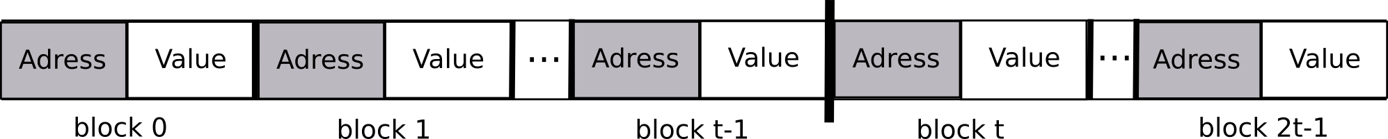
Figure 1. Address and value bits of blocks.

Function $\mathtt{2\mbox{-}SAF}_{t}(X)$ is calculated based on the following five sub-routines:

1. $Adr:\{0,1\}^{n}\times\{0,\dots,2t-1\}\to\{0,\dots,2t-1\}$ gets the address of a block:

   $$Adr(X,p)=\sum_{j=0}^{\lceil\log 2t\rceil-1}y^{p}_{j}\cdot 2^{j}(mod\textrm{ }2t).$$

2. $Ind:\{0,1\}^{n}\times\{0,\dots,2t-1\}\to\{-1,\dots,2t-1\}$ gets the number of block by address:

   $$Ind(X,a)=\left\{\begin{array}[]{ccl}p&,&\textrm{where $p$ is the minimal number such that $Adr(X,p)=a$},\\ -1&,&\textrm{if there are no such $p$}\end{array}\right..$$

3. $Val:\{0,1\}^{n}\times\{0,\dots,2t-1\}\to\{-1,\dots,t-1\}$ gets the value of the block with address $i$:

   $$Val(X,a)=\left\{\begin{array}[]{ccl}\sum_{j=0}^{b-1}x^{p}_{j}(mod\textrm{ }t)&,&\textrm{where }p=Ind(X,a)\textrm{ for $p\geq 0$},\\ -1&,&\textrm{if }Ind(X,a)<0\end{array}\right..$$

Suppose that we are at the $i$-th step of iteration.

1. $Step_{1}:\{0,1\}^{n}\times\{0,\dots,1\}\to\{-1,t\dots,2t-1\}$ gets the first part of the $i$th step of iteration:

   $$Step_{1}(X,i)=\left\{\begin{array}[]{ccl}-1&,&\textrm{if }Step_{2}(X,i-1)=-1,\\ Val(X,Step_{2}(X,i-1))+t&,&\textrm{otherwise}\end{array}\right..$$

2. $Step_{2}:\{0,1\}^{n}\times\{-1,\dots,1\}\to\{-1,\dots,t-1\}$ gets the second part of the $i$th step of iteration:

   $$Step_{2}(X,i)=\left\{\begin{array}[]{ccl}-1&,&\textrm{if }Step_{1}(X,i)=-1,\\ 2&,&\textrm{if }i=-1\\ Val(X,Step_{1}(X,i))&,&\textrm{otherwise}\end{array}\right..$$

Function $\mathtt{2\mbox{-}SAF}_{t}(X)$ is computed iteratively: $\mathtt{2\mbox{-}SAF}_{t}(X)=\left\{\begin{array}[]{ll}0,&\textrm{if }Step_{2}(X,1)\leq 0,\\ 1,&\textrm{otherwise }\end{array}\right.:$

1. We find the block with address $2$ in the first part and compute the value of this block, which is the address of the block for the second part.

2. We take the block from the second part with the computed address and compute value of the block, which is the address of the new block for the first part.

3. We find the block with new address in the second part and check value of this block. If the value is greater than $0$, then value of $\mathtt{2\mbox{-}SAF}_{t}$ is $1$, and $0$ otherwise.

If we do not find block with searching address $n$ in any phase then value of $\mathtt{2\mbox{-}SAF}_{t}$ is also $0$. See the Figure 2 for the iterations of the function.

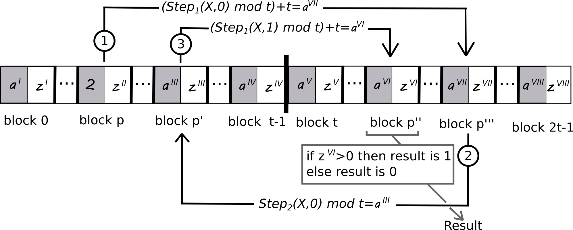
Figure 2. $\mathtt{2\mbox{-}SAF}_{t}(X)$, $Step_{1}(X,i)$ and $Step_{2}(X,i)$ functions. In the picture we write $a$ in address bits of $p$-th block (gray box) if $A(X,p)=a$.

Theorem 5.

For integer $t=t(n)$, $N(\mathtt{2\mbox{-}SAF}_{t})\geq t^{t-2},$ where $t$ satisfies $2t(2t+\lceil\log 2t\rceil)<n$.

Proof.

The proof is based on the following two technical Lemmas 3 and 4.

Lemma 3.

Let $t=t(n)$ be some integers satisfying Inequality (1) and $\pi=(X_{A},X_{B})$ be a partition such that $X_{A}$ contains at least $t$ value variables from exactly $t$ blocks. Then, $X_{B}$ contains at least $t$ value variables from exactly $t$ blocks.

Proof.

We define $I_{A}=\{i:$ $X_{A}$ contains at least $t$ value variables from $i$th block$\}$. Let $i^{\prime}\not\in I_{A}$. Then, $X_{A}$ contains at most $t-1$ value variables from $i^{\prime}$th block, so $X_{B}$ contains at least $b-(t-1)$ value variables from $i^{\prime}$th block. By (1), we can get

$$b-(t-1)=\left\lfloor\frac{n}{2t}\right\rfloor-\lceil\log 2t\rceil-(t-1)$$

which is bigger than

$$(2t+\lceil\log 2t\rceil)-\lceil\log 2t\rceil-(t-1)=2t-(t-1)=t+1.$$

Let $I=\{0,\dots,2t-1\}$ be the numbers of all blocks and $i^{\prime}\in I\backslash I_{A}$. Then, we can follow that $|I\backslash I_{A}|=2t-t=t$. ∎

Let $\theta\in\Theta(n)$ be any order. Then, we pick a partition $\pi=(X_{A},X_{B})\in\Pi(\theta)$ such that $X_{A}$ contains at least $t$ value variables from exactly $t$ blocks. We define $I_{A}=\{i:$ $X_{A}$ contains at least $t$ value variables from $i$th block$\}$ and $I_{B}=\{0,\dots,2t-1\}\backslash I_{A}$. By the proof of Lemma 3, we know that $|I_{B}|=t$.

Let $(\sigma,\gamma)$ be the partition for the input $\nu$ with respect to $\pi$. We define the sets $\Psi\subset\{{0,1\}^{|X_{A}|}}$ and $\Gamma\subset\{{0,1\}^{|X_{B}|}}$ for the input $\nu$ with respect to $\pi$ that satisfies the following conditions. For $\sigma,\sigma^{\prime}\in\Psi$, $\gamma\in\Gamma$, $\nu=(\sigma,\gamma)$, and $\nu^{\prime}=(\sigma^{\prime},\gamma)$:

• For any $z\in\{0,\dots,t-1\}$, $Ind(\nu,z)\in I_{A}$;

• For any $z\in\{w,\dots,2t-1\}$, $Ind(\nu,z)\in I_{B}$;

• There is $z\in\{2,\dots,t-1\}$ such that $Val(\nu^{\prime},z)\neq Val(\nu,z)$;

• The value of $x^{p}_{j}$ is $0$ for any $p\in I_{B}$ and $x^{p}_{j}\in X_{A}$;

• The value of $x^{p}_{j}$ is $0$ for any $p\in I_{A}$ and $x^{p}_{j}\in X_{B}$;

• $Val(\nu,0)=2t-2,Val(\nu^{\prime},1)=2t-1;\mbox{ and,}$

• $Val(\nu,2t-2)=0,Val(\nu,2t-1)=1.$

Lemma 4.

For any sequence $(a_{2},\dots,a_{2t-3})$, where $a_{i}\in\{0,\dots,t-1\}$, there are $\sigma\in\Psi$ and $\gamma\in\Gamma$ such that $Val(\nu,z_{i})=a_{i}$ for $z_{i}\in\{2,\dots,t-1\}$ and $i\in\{2,\dots,2t-3\}$.

Proof.

Let $p_{i}\in I_{A}$ such that $p_{i}=Ind(\nu,z_{i})$ for $i\in\{2,\dots,t-1\}$. Remember that the value of $x^{p_{i}}_{j}$ is $0$ for any $x^{p_{i}}_{j}\in X_{B}$. Hence the value of $Val(\nu,z_{i})$ depends only on the variables from $X_{A}$. At least $t$ value variables of $p_{i}$th block belong to $X_{A}$. Hence we can choose input with $a_{i}$ $1$’s in the value variables of $p_{i}$th block which belongs to $X_{A}$. For set $\Gamma$ and $i\in\{t,\dots,2t-3\}$, we can follow the same proof. ∎

Remember the statement of the theorem: For integer $t=t(n)$, if $\mathtt{2\mbox{-}SAF}_{t}$ satisfies Inequality (1), then

$$N(\mathtt{2\mbox{-}SAF}_{t})\geq t^{t-2}.$$

Here are the details for the proofs.

Let $\theta\in\Theta(n)$ be an order. Then, we pick the partition $\pi=(X_{A},X_{B})\in\Pi(\theta)$ such that $X_{A}$ contains at least $t$ value variables from exactly $t$ blocks.

Let $\sigma,\sigma^{\prime}\in\Psi$ be two different inputs and $\tau$ and $\tau^{\prime}$ be their corresponding mappings, respectively. We show that the subfunctions $\mathtt{2\mbox{-}SAF_{t}}|_{\tau}$ and $\mathtt{2\mbox{-}SAF_{t}}|_{\tau^{\prime}}$ are different. Let $z\in\{2,\dots,t-1\}$ such that $s^{\prime}=Val(\nu^{\prime},z)\neq Val(\nu,z)=s$.

If $z>2$, then we choose $\gamma\in\Gamma$ providing that $Val(\nu,s+t)=1$, $Val(\nu^{\prime},s^{\prime}+t)=0$, and $Val(\nu,r)=Val(\nu^{\prime},r)=z$, where $r=Val(\nu,2)$. That is,

• $Step_{1}(\nu,0)=Step_{1}(\nu^{\prime},0)=r$,

• $Step_{2}(\nu,0)=s$ and $Step_{2}(\nu^{\prime},0)=s^{\prime}$,

• $Step_{1}(\nu,1)=2t-1$ and $Step_{1}(\nu^{\prime},1)=2t-2$, and,

• $Step_{2}(\nu,1)=1$ and $Step_{2}(\nu^{\prime},1)=0$.

Thus, $\mathtt{2\mbox{-}SAF}_{t}(\nu)=1$ and $\mathtt{2\mbox{-}SAF}_{t}(\nu^{\prime})=0$.

If $z=2$, then we choose $\gamma\in\Gamma$ providing that $Val(\nu,s+t)=1$ and $Val(\nu^{\prime},s^{\prime}+t)=0$. That is,

• $Step_{1}(\nu,0)=s$ and $Step_{1}(\nu^{\prime},0)=s^{\prime}$,

• $Step_{2}(\nu,1)=1$ and $Step_{2}(\nu^{\prime},1)=0$,

• $Step_{1}(\nu,1)=2t-1$ and $Step_{1}(\nu^{\prime},1)=2t-2$, and,

• $Step_{2}(\nu,1)=1$ and $Step_{2}(\nu^{\prime},1)=0$.

Hence $\mathtt{2\mbox{-}SAF}_{t}(\nu)=1$ and $\mathtt{2\mbox{-}SAF}_{t}(\nu^{\prime})=0$.

Therefore $\mathtt{2\mbox{-}SAF}_{t}|_{\tau}(\gamma)\neq\mathtt{2\mbox{-}SAF}_{t}|_{\tau^{\prime}}(\gamma)$ and also $\mathtt{2\mbox{-}SAF}_{t}|_{\tau}\neq\mathtt{2\mbox{-}SAF}_{t}|_{\tau^{\prime}}$.

Now, we compute $|\Psi|$. For $\sigma\in\Psi$, we can get each value of $Val(\nu,i)$ for $2\leq i\leq t-1$. It means $|\Psi|\geq t^{t-2}$ due to Lemma 4. Therefore, $N^{\pi}(\mathtt{2\mbox{-}SAF}_{t})\geq t^{t-2}$, and, by definition of $N(\mathtt{2\mbox{-}SAF}_{t})$, we have $N(\mathtt{2\mbox{-}SAF}_{t})\geq t^{t-2}$. ∎

Theorem 6.

There is a $2DA_{n}$ $A_{n}$ of size $13t+4$ that computes $\mathtt{2\mbox{-}SAF}_{t}$.

Proof.

Let $\nu\in\{0,1\}^{n}$ be the input. We begin with the first part of automaton $A_{n}$ that computes $Step_{1}(X,0)$. Automaton $A_{n}$ checks each $j$th block for predicate $Adr(\nu,j)=2$. If it is true, then $A_{n}$ computes $Val(\nu,2)=r^{\prime}$, and, it checks the next block, otherwise. If $A_{n}$ checks all blocks and does not find the block, it switches to the rejecting state. If $A_{n}$ finds $r^{\prime}$, then it goes to one of the special state $s^{\prime}_{r^{\prime}}$. From this state, the automaton returns back to the beginning of the input.

We continue with the second part of automaton $A_{n}$ that computes $Step_{2}(X,0)$. From the state $s^{\prime}_{r^{\prime}}$, $A_{n}$ checks each $j$th block for predicate $Adr(\nu,j)=r^{\prime}$. If it is true, then $A_{n}$ computes $Val(\nu,r^{\prime})=r^{\prime\prime}$, and, it checks the next block, otherwise. If $A_{n}$ checks all blocks and does not find the block, it switches to the rejecting state. If $A_{n}$ finds $r^{\prime\prime}$, then it goes to one of special state $s^{\prime\prime}_{r^{\prime\prime}}$. From this state, the automaton returns back to the beginning of the input.

Now, we describe the third part of automaton $A_{n}$ that computes $Step_{1}(X,1)$. From the state $s^{\prime\prime}_{r^{\prime\prime}}$, $A_{n}$ checks each $j$th block for predicate $Adr(\nu,j)=r^{\prime\prime}$. If it is true, then $A_{n}$ computes $Val(\nu,r^{\prime\prime})=r^{\prime\prime\prime}$, and, it checks the next block, otherwise. If $A_{n}$ checks all blocks and does not find the block, then it switches to the rejecting state. If $A_{n}$ finds $r^{\prime\prime\prime}$, then it goes to one of special state $s^{\prime\prime\prime}_{r^{\prime\prime\prime}}$. From this state automaton returns back to the beginning of the input.

The forth part of automaton $A_{n}$ computes $Step_{2}(X,1)$. From the state $s^{\prime\prime\prime}_{r^{\prime\prime\prime}}$, $A_{n}$ checks each $j$th block for predicate $Adr(\nu,j)=r^{\prime\prime\prime}$. If it is true, then $A_{n}$ computes $Val(\nu,r^{\prime\prime\prime})=r^{IV}$, and, it checks next block otherwise. If $A_{n}$ checks all blocks and does not find the block, it switches to the rejecting state. If $A_{n}$ finds $r^{IV}$ and $r^{IV}=1$, the automaton accepts the input and rejects the input, otherwise.

In the first part, the block checking procedure uses only $2$ states. Computing $Val(\nu,2)$ uses $w$ states and there are $t$ $s^{\prime}_{r^{\prime}}$ states. So, the size of the first part is $2+2t$. In the second part, the block checking procedure uses only $2$ states and we have $t$ blocks to check the state pairs for each value of $r^{\prime}$, that is $2t$ states. Computing $Val(\nu,r^{\prime})$ uses $t$ states and also $A_{n}$ has $t$ $s^{\prime\prime}_{r^{\prime\prime}}$ states. Therefore, the size of the second part is $4t$. Similarly, we can show that the size of the third part is $4t$. In the fourth part, we need $3t$ states for procedure checking and computing $Val(\nu,r^{\prime\prime\prime})$. $A_{n}$ has also one accept and one reject states. So, the size of the forth part is $3t+2$. Thus, the overall size of $A_{n}$ is $13t+4$. ∎

3.2.2. Boolean Function $\mathtt{2\mbox{-}USAF}_{t}$:

The definition of $\mathtt{2\mbox{-}USAF_{t}}$ is as follows:

$$\mathtt{2\mbox{-}USAF}_{t}(X):\{0,1\}^{n}\to\{0,1\}\mbox{ for integer $t=t(n)$ satisfying that }$$

(2) $$4t(2t+\lceil\log 2t\rceil)<n.$$

We denote its language version as $\mathtt{L2USAF}_{t}$.

We divide the input variables (the symbols of the input) into $2t$ blocks. There are $\left\lfloor\frac{n}{2t}\right\rfloor=q$ variables in each block. After that, we divide each block into mark, address, and value variables. All variables that are in odd positions are mark. The type of the bit on an even position is determined by the value of previous mark bit. The bit is address, if the previous mark bit’s value is 0, and value otherwise. The first $\lceil\log 2t\rceil=c$ variables of block that are in the even positions denote the address and the other $q/2-\lceil\log 2t\rceil=b$ variables of block denote the value.

We call $x^{p}_{0},\dots,x^{p}_{b-1}$, $y^{p}_{0},\dots,y^{p}_{\lceil\log 2t\rceil}$ and $z^{p}_{0},\dots,z^{p}_{q/2}$ are the value, address, and the mark variables of the $p$th block, respectively, for $p\in\{0,\dots,2t-1\}$.

Function $\mathtt{2\mbox{-}USAF}_{t}(X)$ is calculated based on the following five sub-routines:

1. $Adr:\{0,1\}^{n}\times\{0,\dots,2t-1\}\to\{0,\dots,2t-1\}$ gets the address of a block:

   $$Adr(X,p)=\sum_{j=0}^{c-1}y^{p}_{j}\cdot 2^{c-j-1}(mod\textrm{ }2t).$$

2. $Ind:\{0,1\}^{n}\times\{0,\dots,2t-1\}\to\{-1,\dots,2t-1\}$ gets the number of block by address:

   $$Ind(X,a)=\left\{\begin{array}[]{ccl}p&,&\textrm{where $p$ is the minimal number such that $Adr(X,p)=a$},\\ -1&,&\textrm{if there are no such $p$}\end{array}\right..$$

3. $Val:\{0,1\}^{n}\times\{0,\dots,2t-1\}\to\{-1,\dots,t-1\}$ gets the value of the block with address $i$:

   $$Val(X,a)=\left\{\begin{array}[]{ccl}\sum_{j=0}^{b-1}x^{p}_{j}(mod\textrm{ }t)&,&\textrm{where }p=Ind(X,a)\textrm{ for $p\geq 0$},\\ -1&,&\textrm{if }Ind(X,i)<0\end{array}\right..$$

Suppose that we are at the $i$-th step of iteration.

1. $Step_{1}:\{0,1\}^{n}\times\{0,\dots,1\}\to\{-1,t\dots,2t-1\}$ gets the first part of the $i$th step of iteration:

   $$Step_{1}(X,i)=\left\{\begin{array}[]{ccl}-1&,&\textrm{if }Step_{2}(X,i-1)=-1,\\ Val(X,Step_{2}(X,i-1))+t&,&\textrm{otherwise}\end{array}\right..$$

2. $Step_{2}:\{0,1\}^{n}\times\{-1,\dots,1\}\to\{-1,\dots,t-1\}$ gets the second part of the $i$th step of iteration:

   $$Step_{2}(X,i)=\left\{\begin{array}[]{ccl}-1&,&\textrm{if }Step_{1}(X,i)=-1,\\ 2&,&\textrm{if }i=-1\\ Val(X,Step_{1}(X,i))&,&\textrm{otherwise}\end{array}\right..$$

Remark that the address of the current block is computed on the previous step. Function $\mathtt{2\mbox{-}USAF}_{t}(X)$ is computed as: $\mathtt{2\mbox{-}USAF}_{t}(X)=\left\{\begin{array}[]{ll}0,&\textrm{if }Step_{2}(X,1)\leq 0,\\ 1,&\textrm{otherwise }\end{array}\right..$

Theorem 7.

For integer $t=t(n)$, $R_{n}(\mathtt{L2USAF}_{t})\geq t^{t-2},$ where $t$ satisfies $4t(2t+\lceil\log 2t\rceil)<n$.

Proof.

We pick the partition $\pi=(X_{A},X_{B})\in\Pi(id)$ such that $X_{A}$ contains exactly $w$ blocks.

Let $\sigma,\sigma^{\prime}\in\Psi$ be two different inputs and $\tau$ and $\tau^{\prime}$ be their corresponding mappings, respectively. We show that the subfunctions $\mathtt{2\mbox{-}USAF_{t}}|_{\tau}$ and $\mathtt{2\mbox{-}USAF_{t}}|_{\tau^{\prime}}$ are different. Let $z\in\{2,\dots,t-1\}$ such that $s^{\prime}=Val(\nu^{\prime},z)\neq Val(\nu,z)=s$.

If $z>2$, then we choose $\gamma\in\Gamma$ providing that $Val(\nu,s+t)=1$, $Val(\nu^{\prime},s^{\prime}+t)=0$, and $Val(\nu,r)=Val(\nu^{\prime},r)=z$, where $r=Val(\nu,2)$. That is,

• $Step_{1}(\nu,0)=Step_{1}(\nu^{\prime},0)=r$,

• $Step_{2}(\nu,0)=s$ and $Step_{2}(\nu^{\prime},0)=s^{\prime}$,

• $Step_{1}(\nu,1)=2t-1$ and $Step_{1}(\nu^{\prime},1)=2t-2$, and,

• $Step_{2}(\nu,1)=1$ and $Step_{2}(\nu^{\prime},1)=0$.

Thus, $\mathtt{2\mbox{-}USAF_{t}}(\nu)=1$ and $\mathtt{2\mbox{-}USAF_{t}}(\nu^{\prime})=0$.

If $z=2$, then we choose $\gamma\in\Gamma$ providing that $Val(\nu,s+t)=1$ and $Val(\nu^{\prime},s^{\prime}+t)=0$. That is,

• $Step_{1}(\nu,0)=s$ and $Step_{1}(\nu^{\prime},0)=s^{\prime}$,

• $Step_{2}(\nu,1)=1$ and $Step_{2}(\nu^{\prime},1)=0$,

• $Step_{1}(\nu,1)=2t-1$ and $Step_{1}(\nu^{\prime},1)=2t-2$, and,

• $Step_{2}(\nu,1)=1$ and $Step_{2}(\nu^{\prime},1)=0$.

Hence $\mathtt{2\mbox{-}USAF_{t}}(\nu)=1$ and $\mathtt{2\mbox{-}USAF_{t}}(\nu^{\prime})=0$.

Therefore $\mathtt{2\mbox{-}USAF_{t}}|_{\tau}(\gamma)\neq\mathtt{2\mbox{-}USAF_{t}}|_{\tau^{\prime}}(\gamma)$ and also $\mathtt{2\mbox{-}USAF_{t}}|_{\tau}\neq\mathtt{2\mbox{-}USAF_{t}}|_{\tau^{\prime}}$.

Now, we compute $|\Psi|$. For $\sigma\in\Psi$, we can get each value of $Val(\nu,i)$ for $2\leq i\leq t-1$. It means $|\Psi|\geq t^{t-2}$ due to Lemma 4. Therefore, $N^{\pi}(\mathtt{2\mbox{-}USAF_{t}})\geq t^{t-2}$, and, by definition of $N(\mathtt{2\mbox{-}USAF_{t}})$, we have $N(\mathtt{2\mbox{-}USAF_{t}})\geq t^{t-2}$. ∎

Theorem 8.

There is a $2DFA$ $A_{n}$ of size $23t+2(1+3t)\log{t}+6$ recognizing $\mathtt{L2USAF}_{t}$.

Proof.

The computation of $A_{n}$ consists of four parts similar to the automaton given in Theorem 6.

In the first part, the block checking procedure uses $2\log{2t}+2$ states. Computing $Val(\nu,2)$ uses $2t$ states and there are $w$ $s^{\prime}_{r^{\prime}}$ states. So, the size of the first part is $3t+2\log{2t}+2$. In the second part, the block checking procedure uses $2\log{2t}+2$ states and we have $t$ blocks to check the state pairs for each value of $r^{\prime}$, that is $w(2\log{2t}+2)$ states. Computing $Val(\nu,r^{\prime})$ uses $2t$ states and also $A_{n}$ has $t$ $s^{\prime\prime}_{r^{\prime\prime}}$ states. Therefore, the size of the second part is $5t+2t\log{2t}$. Similarly, we can show that the size of the third part is $5t+2t\log{2t}$. In the fourth part, we use $4t+2t\log{2t}$ states for procedure checking and computing $Val(\nu,r^{\prime\prime\prime})$. $A_{n}$ has also one accept and one reject states. So, the size of the forth part is $4t+2t\log{2t}+2$. Thus, the overall size of $A_{n}$ is $23t+2(1+3t)\log{t}+6$. ∎

We can simplify the formula for the number of states for bigger $t$ values, e.g.:

• For $t>2906$, there is a $2DFA$ of size $8t\log(t)$ recognizing $\mathtt{L2USAF}_{t}$.

• For $t>26$, there is a $2DFA$ of size $11t\log(t)$ recognizing $\mathtt{L2USAF}_{t}$.

• For $t>3$, there is a $2DFA$ of size $19t\log(t)$ recognizing $\mathtt{L2USAF}_{t}$.

4. Hierarchies results

Now, we can follow our hierarchies and incomparability results.

Theorem 9.

Let $d:\mathbb{N}\rightarrow\mathbb{N}$ be a function satisfying $13d+43<\sqrt{\frac{n}{6}}$. Then, $\mathsf{2D\Theta SIZE(\mathrm{d})}\subsetneq\mathsf{2D\Theta SIZE(\mathrm{13d+43})}.$

Proof.

By Theorem 5, we can follow that $(d+1)^{d+1}<(d+3)^{d+1}\leq N(\mathtt{2\mbox{-}SAF}_{d+3}).$ Suppose that there is a $2DA^{\Theta}_{n}$ with size $d$ computing $\mathtt{2\mbox{-}SAF}_{d+3}$. Then, by Theorem 1, we can have $N(\mathtt{2\mbox{-}SAF}_{d+3})\leq(d+1)^{d+1},$ which is a contradiction and so $\mathtt{2\mbox{-}SAF}_{d+3}\notin\mathsf{2D\Theta SIZE(\mathrm{d})}$.

Moreover, by Theorem 6, we have that $\mathtt{2\mbox{-}SAF}_{d+3}$ is in $\mathsf{2DSIZE(\mathrm{13d+43})}$.

Lastly, the relation between $d$ and $n$ can be followed from the definition of $\mathtt{2\mbox{-}SAF}_{d}$ by also taking into account the parameter $(13d+43)$. For $\mathtt{2\mbox{-}SAF}_{t}$, we have inequality $2t(2t+\lceil\log(2t)\rceil)<n$. For $t\geq 2$, we always have $t\geq\lceil\log(2t)\rceil$. Therefore, the following inequality also works $2t(3t)<n$, which gives us that $t<\sqrt{\frac{n}{6}}$. ∎

Theorem 10.

Let $d:\mathbb{N}\rightarrow\mathbb{N}$ be a function satisfying $121<13d(n)+4<\sqrt{\frac{n}{6}}$. Then, $\mathsf{2N\Theta SIZE(\mathrm{\lfloor\sqrt{d}\rfloor})}\subsetneq\mathsf{2N\Theta SIZE(\mathrm{13d+4})}.$

Proof.

By Theorem 5 we have $2^{\log_{2}d(d-2)}=d^{d-2}\leq N(\mathtt{2\mbox{-}SAF}_{d}).$ For $d>9$, we can follow that

$$2^{(\sqrt{d}+1)^{2}}<2^{\log_{2}d(d-2)}.$$

Suppose that there is a $2NA^{\Theta}_{n}$ with size $\lfloor\sqrt{d}\rfloor$ computing $\mathtt{2\mbox{-}SAF}_{d}$. Then, by Theorem 2, we can have $N(\mathtt{2\mbox{-}SAF}_{d})\leq 2^{(\lfloor\sqrt{d}\rfloor+1)^{2}},$ which is a contradiction and so $\mathtt{2\mbox{-}SAF}_{d}\notin\mathsf{2N\Theta SIZE(\mathrm{\lfloor\sqrt{d}\rfloor})}$.

Moreover, by Theorem 6, we have that $\mathtt{2\mbox{-}SAF}_{d}$ is in $\mathsf{2DSIZE(\mathrm{13d+4})}$.

The relation between $d$ and $n$ can be followed similar to the previous proof and the condition $d>9$. ∎

Theorem 11.

Let $d:\mathbb{N}\rightarrow\mathbb{N}$ be a function satisfying $1330<\lceil 11d(n)\log d(n)\rceil<\sqrt{\frac{n}{12}}$. Then, $\mathsf{2DFASIZE(\mathrm{d-3})}\subsetneq\mathsf{2DFASIZE(\mathrm{\lceil 11d\log d\rceil})}$.

Proof.

By Theorem 7, we have $(d-2)^{d-2}<d^{d-2}\leq N(\mathtt{2\mbox{-}USAF}_{d})$ and so we can also have

$$(d-2)^{d-2}<R_{n}(\mathtt{L2USAF}_{d}).$$

Suppose that there is a 2DFA with size $d-3$ recognizing $\mathtt{L2USAF}_{d}$. Then, by Corollary 1, we can have $R_{n}(\mathtt{L2USAF}_{d})\leq(d-2)^{d-2},$ which is a contradiction and so $\mathtt{L2USAF}_{d}\notin\mathsf{2DFASIZE(\mathrm{d-3})}.$

By Theorem 8 and for $d>26$, we have $\mathtt{L2USAF}_{d}\in\mathsf{2DFASIZE(\mathrm{\lceil 11d\log d\rceil})}$.

The relation between $d$ and $n$ can be followed by the definition of $\mathtt{2\mbox{-}USAF}_{t}$: $4t(2t+\lceil\log(2t)\rceil)<n$. For $t\geq 2$, $t\geq\lceil\log(2t)\rceil$ and so we can also use the inequality $4t(3t)<n$, which implies $t\leq\sqrt{\frac{n}{12}}$. ∎

Theorem 12.

Let $d:\mathbb{N}\rightarrow\mathbb{N}$ be a function satisfying $1330<\lceil 11d\log d\rceil<\sqrt{\frac{n}{12}}$. Then, $\mathsf{2NFASIZE(\mathrm{\lfloor\sqrt{d}\rfloor})}\subsetneq\mathsf{2NFASIZE(\mathrm{\lceil 11dlogd\rceil})}$.

Proof.

By using the facts given in the two above proofs, for $d>9$, we know that $\mathtt{L2USAF}_{d}\notin\mathsf{2NFASIZE(\mathrm{\lfloor\sqrt{d}\rfloor})}$ and $\mathtt{L2USAF}_{d}\in\mathsf{2DFASIZE(\mathrm{\lceil 11d\log d\rceil})}.$ ∎

Theorem 13.

Let $d:\mathbb{N}\rightarrow\mathbb{N}$ be a function satisfying $30<13d(n)+4<\sqrt{\frac{n}{6}}$ and $T\geq 256$ be the expected running time to finish computation. Then

$$\mathsf{2B\Theta SIZE\left(\mathrm{\left\lfloor\frac{\sqrt{d}}{32\log T}\right\rfloor}\right)}\subsetneq\mathsf{2B\Theta SIZE\left(\mathrm{13d+4}\right)},$$

where the error bound is at least $\frac{1}{5}$ for the classes.

Proof.

By using Theorem 5, we can obtain the following for $d>2$.

$$\left(\frac{32\log(T)\sqrt{d}}{32\log(T)}\right)^{\left(\frac{\sqrt{d}}{32\log T}+1\right)^{2}}<\left(\frac{32\log(T)d}{32\log(T)}\right)^{d-2}=d^{d-2}\leq N(\mathtt{2\mbox{-}SAF}_{d}).$$

Then $\mathtt{2\mbox{-}SAF}_{d}$ cannot be solved by a $2PA^{\Theta}_{n}$ with size $\lfloor\frac{\sqrt{d}}{32\log T}\rfloor$. Otherwise, by Corollary 1, we obtain the following contradiction.

$$N(\mathtt{2\mbox{-}SAF}_{d})<\left(32\log T\left\lfloor\frac{\sqrt{d}}{32\log T}\right\rfloor\right)^{\left(\lfloor\frac{\sqrt{d}}{32\log T}\rfloor+1\right)^{2}}.$$

By Theorem 6, we have that $\mathtt{2\mbox{-}SAF}_{d}$ is in $\mathsf{2DSIZE(\mathrm{13d+4})}$.

The relation between $d$ and $n$ can be followed similar to the previous proofs and the condition $d>2$. ∎

5. Incomparability results

In this section, we give evidences how shuffling can reduce the size of models. For this purpose, we use the well-known Equality function

$$\mathtt{EQ}(X)=\bigvee_{0}^{\lfloor n/2\rfloor-1}x_{i}=x_{i+\lfloor n/2\rfloor}.$$

The nice property of $\mathtt{EQ}(X)$ for our purpose is that $N^{id}(\mathtt{EQ})=2^{\lfloor n/2\rfloor}$ and $N^{\theta}(\mathtt{EQ})\leq 4$ for $\theta=(0,\lfloor n/2\rfloor,1,\lfloor n/2\rfloor+1,\dots)$. Therefore, we can follow that $\mathsf{\mathtt{EQ}}\in\mathsf{2D\Theta SIZE(\mathrm{4})}$.

Suppose that there is a $2NA_{n}$ with size $\lfloor\sqrt{\frac{n}{2}}\rfloor-2$ solving $\mathtt{EQ}$. Then, by Theorem 2, we have

$$N^{id}(\mathtt{EQ})\leq 2^{(\lfloor\sqrt{\frac{n}{2}}\rfloor-1)^{2}},$$

which is a contradiction. Therefore, $\mathtt{EQ}\notin\mathsf{2NSIZE(\mathrm{\lfloor\sqrt{\frac{n}{2}}\rfloor-2})}$. We use this lower bound also for deterministic case.

Let $d=d(n)$ be a function such that $d\leq\lfloor\sqrt{\frac{n}{2}}\rfloor-2$, and $d^{\prime}$ be a function such that $4\leq d^{\prime}<d$. Then, due to the fact given for function $\mathtt{EQ}$, we can immediately follow that

$$\mathsf{2D\Theta SIZE(\mathrm{d^{\prime}})}\notin\mathsf{2DSIZE(\mathrm{d})}~{}~{}\mbox{ and }~{}~{}\mathsf{2N\Theta SIZE(\mathrm{d^{\prime}})}\notin\mathsf{2NSIZE(\mathrm{d})}.$$

On the other hand, due to the results given in Section 4, the shuffling classes cannot contain the non-shuffling classes under certain size bounds, which leads us to our incomparability results.

Theorem 14.

As a further restriction, if $13d+43<\sqrt{\frac{n}{6}}$, then for $94\leq 13d^{\prime}+43<d$, the classes $\mathsf{2D\Theta SIZE(\mathrm{d^{\prime}})}$ and $\mathsf{2DSIZE(\mathrm{d})}$ are not comparable.

Proof.

By the proof of Theorem 9, we know that $\mathsf{2D\Theta SIZE(\mathrm{d^{\prime}})}$ does not have a function that is in $\mathsf{2DSIZE(\mathrm{13d^{\prime}+43})}$. Since $13d^{\prime}+43<d$, this function is also in $\mathsf{2DSIZE(\mathrm{d})}$. ∎

Theorem 15.

As a further restriction, if $121<13d+4<\sqrt{\frac{n}{6}}$, then for $58\leq 13d^{\prime}+4<d$, the classes $\mathsf{2N\Theta SIZE(\mathrm{\lfloor\sqrt{d^{\prime}}\rfloor})}$ and $\mathsf{2NSIZE(\mathrm{d})}$ are not comparable.

Proof.

By the proof of Theorem 10, we know that $\mathsf{2N\Theta SIZE(\mathrm{\lfloor\sqrt{d^{\prime}}\rfloor})}$ does not have a function that is in $\mathsf{2DSIZE(\mathrm{13d^{\prime}+4})}$. Since $13d^{\prime}+4<d$, this function is also in $\mathsf{2NSIZE(\mathrm{d})}$. ∎

Any $2PA_{n}$ with size $d$ satisfying $\left(32d\log T\right)^{(d+1)^{2}}<2^{\lfloor\frac{n}{2}\rfloor}$ cannot solve $\mathtt{EQ}$ due to Theorem 4. We bound $T<2^{2^{d}}$. Then, for $d\geq 2$, we can follow

$$\left(32d\log T\right)^{(d+1)^{2}}<\left(2^{5}2^{\log_{2}d}2^{d}\right)^{(d+1)^{2}}\leq\frac{2^{d^{3}}}{2}<\frac{2^{\frac{n}{2}}}{2}<2^{\lfloor\frac{n}{2}\rfloor}.$$

Then, for $4\leq d^{\prime}\leq d$ where $d<\sqrt[3]{\frac{n}{2}}$, $\mathsf{2B\Theta SIZE\left(\mathrm{d^{\prime}}\right)}\notin\mathsf{2BSIZE(\mathrm{d})}$. Now, we can state the result for probabilistic case similar to the other cases.

Theorem 16.

As a further restriction, if $30<13d+4<\sqrt[3]{\frac{n}{2}}$, then for $4\leq 13d^{\prime}+4<d$ and $256\leq T<2^{2^{d^{\prime}}}$ be the expected running time to finish computation, the classes $\mathsf{2B\Theta SIZE\left(\mathrm{\left\lfloor\frac{\sqrt{d^{\prime}}}{32\log T}\right\rfloor}\right)}$ and $\mathsf{2BSIZE(\mathrm{d})}$ are not comparable.

Acknowledgements.

The authors thank to A. Ambainis, A. Rivosh, K. Prūsis, and J. Vihrovs for useful discussions and comments.

The work is partially supported by ERC Advanced Grant MQC. The work is performed according to the Russian Government Program of Competitive Growth of Kazan Federal University

References

- [1] F. Ablayev, A. Gainutdinova, K. Khadiev, and A. Yakaryılmaz. Very narrow quantum OBDDs and width hierarchies for classical OBDDs. Lobachevskii Journal of Mathematics, 37(6):670–682, 2016.
- [2] Farid Ablayev, Aida Gainutdinova, Kamil Khadiev, and Abuzer Yakaryılmaz. Very narrow quantum OBDDs and width hierarchies for classical OBDDs. In DCFS, volume 8614 of LNCS, pages 53–64. Springer, 2014.
- [3] Farid Ablayev and Kamil Khadiev. Extension of the hierarchy for k-OBDDs of small width. Russian Mathematics, 53(3):46–50, 2013.
- [4] Farid Ablayev, Andris Ambainis, Kamil Khadiev and Aliya Khadieva. Lower Bounds and Hierarchies for Quantum Memoryless Communication Protocols and Quantum Ordered Binary Decision Diagrams with Repeated Test In SOFSEM 2018, LNCS, 2018 arXiv:1703.05015
- [5] Farid M. Ablayev and Marek Karpinski. On the power of randomized branching programs. In ICALP, volume 1099 of LNCS, pages 348–356. Springer, 1996.
- [6] Kaspars Balodis. One alternation can be more powerful than randomization in small and fast two-way finite automata. In FCT, volume 8070 of LNCS, pages 40–47, 2013.
- [7] David A. Mix Barrington, Howard Straubing, and Denis Thérien. Non-uniform automata over groups. Information and Computation, 89(2):109–132, 1990.
- [8] Beate Bollig, Martin Sauerhoff, Detlef Sieling, and Ingo Wegener. Hierarchy theorems for kOBDDs and kIBDDs. Theoretical Computer Science, 205(1):45–60, 1998.
- [9] Marek Chrobak. Finite automata and unary languages. Theoretical Computer Science, 47(0):149 – 158, 1986.
- [10] Cynthia Dwork and Larry Stockmeyer. A time complexity gap for two-way probabilistic finite-state automata. SIAM Journal on Computing, 19(6):1011–1123, 1990.
- [11] Viliam Geffert, Bruno Guillon, and Giovanni Pighizzini. Two-way automata making choices only at the endmarkers. In Language and Automata Theory and Applications, volume 7183 of LNCS, pages 264–276. Springer Berlin Heidelberg, 2012.
- [12] Markus Holzer. Multi-head finite automata: data-independent versus data-dependent computations. Theoretical Computer Science, 286(1):97–116, 2002.
- [13] Christos A. Kapoutsis. Removing bidirectionality from nondeterministic finite automata. In MFCS, volume 3618 of LNCS, pages 544–555. Springer, 2005.
- [14] Christos A. Kapoutsis. Size complexity of two-way finite automata. In Developments in Language Theory, volume 5583 of LNCS, pages 47–66. Springer, 2009.
- [15] Christos A. Kapoutsis. Nondeterminism is essential in small two-way finite automata with few reversals. Information and Computation, 222(0):208 – 227, 2013. 38th International Colloquium on Automata, Languages and Programming (ICALP 2011).
- [16] Christos A. Kapoutsis, Richard Královic, and Tobias Mömke. Size complexity of rotating and sweeping automata. Journal of Computer and System Sciences, 78(2):537–558, 2012.
- [17] K. Khadiev. Width hierarchy for k-OBDD of small width. Lobachevskii Journal of Mathematics, 36(2):178–183, 2015.
- [18] K. Khadiev. On the hierarchies for deterministic, nondeterministic and probabilistic ordered read-k-times branching programs. Lobachevskii Journal of Mathematics, 37(6):682–703, 2016.
- [19] Kamil Khadiev and Rishat Ibrahimov. Width hierarchies for quantum and classical ordered binary decision diagrams with repeated test. In: Proceedings of the Fourth Russian Finnish Symposium on Discrete Mathematics. No. 26 in TUCS Lecture Notes, Turku Centre for Computer Science (2017)
- [20] Kamil Khadiev and Aliya Khadieva. Reordering method and hierarchies for quantum and classical ordered binary decision diagrams. In Pascal Weil, editor, Computer Science – Theory and Applications: 12th International Computer Science Symposium in Russia, CSR 2017, Kazan, Russia, June 8-12, 2017, Proceedings, volume 10304 of LNCS, pages 162–175. Springer International Publishing, Cham, 2017.
- [21] Hing Leung. Tight lower bounds on the size of sweeping automata. Journal of Computer and System Sciences, 63(3):384 – 393, 2001.
- [22] Noam Nisan and Avi Widgerson. Rounds in communication complexity revisited. In Proceedings of the twenty-third annual ACM symposium on Theory of computing, pages 419–429. ACM, 1991.
- [23] M.O. Rabin and D. Scott. Finite automata and their decision problems. IBM Journal of Research and Development, 3:114–125, 1959.
- [24] William J. Sakoda and Michael Sipser. Nondeterminism and the size of two way finite automata. In STOC’78: Proceedings of the tenth annual ACM symposium on Theory of computing, pages 275–286, 1978.
- [25] John C. Shepherdson. The reduction of two–way automata to one-way automata. IBM Journal of Research and Development, 3:198–200, 1959.
- [26] Moshe Y. Vardi A Note on the Reduction of Two-Way Automata to One-Way Automata. Information Processing Letters, 30(5):261–264, 1989.
- [27] Ingo Wegener. Branching Programs and Binary Decision Diagrams. SIAM, 2000.