THREE NEUTRINO OSCILLATIONS IN MATTER

Abstract

Following similar approaches in the past, the Schrodinger equation for three neutrino propagation in matter of constant density is solved analytically by two successive diagonalizations of 2x2 matrices. The final result for the oscillation probabilities is obtained directly in the conventional parametric form as in the vacuum but with explicit simple modification of two mixing angles ($\theta_{12}$ and $\theta_{13}$) and mass eigenvalues. In this form, the analytical results provide excellent approximation to numerical calculations and allow for simple qualitative understanding of the matter effects.

The MSW effect  MSW for the neutrino propagation in matter attracts a lot of experimental and theoretical attention. Most recently, the discussion is focused on the DUNE experiment  DUNE .

On the theoretical side, a large number of numerical simulations of the MSW effect in matter with a constant or varying density has been performed. Although, in principle, sufficient for comparing the theory predictions with experimental data, they do not provide a transparent physical interpretation of the experimental results. Therefore, several authors have also published analytical or semi-analytical solutions to the Schroedinger equation for three neutrino propagation in matter of constant density, in various perturbative expansions  many papers ; Blennow:2013rca ; Denton:2016wmg . The complexity of the calculation, the transparency of the final result and the range of its applicability depend on the chosen expansion parameter.

In this short note we solve the Schroedinger equation in matter with constant density, using the approximate see-saw structure of the full Hamiltonian in the electroweak basis. This way one can diagonalize the 3x3 matrix by two successive diagonalizations of 2x2 matrices (similar approaches have been used in the past, in particular in ref. Blennow:2013rca and Denton:2016wmg ). We specifically have in mind the parameters of the DUNE experiment but our method is applicable for their much wider range. The final result for the oscillation probabilities is obtained directly in the conventional parametric form as in the vacuum but with modified two mixing angles and mass eigenvalues, similarly to the well known results for the two-neutrino propagation in matter. The three neutrino oscillation probabilities in matter have been presented in the same form as here in the recent ref. PARKE ET AL , where the earlier results obtained in ref. Denton:2016wmg are rewritten in this form. The form of our final results can also be obtained after some simplifications from ref.Blennow:2013rca . Our approach can be easily generalized to non-constant matter density by dividing the path of the neutrino trajectory in the matter to layers and assuming constant density in each layer.

The starting point is the Schroedinger equation

$$i{d\over dx}\nu={\cal H}\nu$$ (1)

where ${\cal H}$ is the Hamiltonian in matter. In the electroweak basis it reads

$${\cal H}=U\left(\begin{array}[]{ccc}0&0&0\\ 0&{\Delta m^{2}_{\odot}\over 2E}&0\\ 0&0&{\Delta m^{2}_{a}\over 2E}\end{array}\right)U^{\dagger}+\left(\begin{array}[]{ccc}V(x)&0&0\\ 0&0&0\\ 0&0&0\end{array}\right)$$ (2)

The matrix $U$ is the neutrino mixing matrix in the vacuum. The mass squared differences are defined as $\Delta m^{2}_{\odot}\equiv m^{2}_{2}-m^{2}_{1}$ ($\approx 7.5\ 10^{-5}eV^{2}$) and $\Delta m^{2}_{a}\equiv m^{2}_{3}-m^{2}_{1}$ ($\approx\pm 2.5\ 10^{-3}eV^{2}$, positive sign is for normal mass ordering and negative sign for inverted one). Here $V(x)$ is the neutrino weak interaction potential energy $V=\sqrt{2}G_{F}N_{e}$ ($N_{e}$ is electron number density) and we take it in this section to be x-independent. The neutrino oscillation probabilities are determined by the $S$-matrix elements

$$S_{\alpha\beta}=T\ e^{-i\int_{x_{0}}^{x_{f}}{\cal H}(x)dx}$$ (3)

For a constant V and in order to obtain our results in the same form as for the oscillation probabilities in the vacuum, it is convenient to rewrite the $S$-matrix elements as follows:

$$S_{\alpha\beta}=e^{-iU_{m}{\cal H}_{m}U^{\dagger}_{m}(x_{f}-x_{0})}=U_{m}e^{-i{\cal H}_{m}L}U^{\dagger}_{m}$$ (4)

The matrix ${\cal H}_{m}$ is the Hamiltonian in matter in the mass eigenstate basis:

$${\left(\begin{tabular}[]{ccc}${\cal H}_{1}$&0&0\\ 0&${\cal H}_{2}$&0\\ 0&0&${\cal H}_{3}$\end{tabular}\right)}$$ (8)

and the $U_{m}$ is the neutrino mixing matrix in matter. Defining $\phi_{21}=({\cal H}_{2}-{\cal H}_{1})L$ and $\phi_{31}=({\cal H}_{3}-{\cal H}_{1})L$, we can write

$$S_{\alpha\beta}=\ \left[U_{m}\left(\begin{array}[]{ccc}1&0&0\\ 0&e^{-i\phi_{21}}&0\\ 0&0&e^{-i\phi_{31}}\end{array}\right)U_{m}^{\dagger}\right]$$ (12)

Here we neglect irrelevant overall phase, $e^{-i{\cal H}_{1}L}$. The neutrino transition probabilities do not depend on the overall phase of the $S$ matrix.

The remaining task is to find the eigenvalues of ${\cal H}$ and the mixing matrix $U_{m}$:

$${\cal H}=U_{m}{\cal H}_{m}U^{\dagger}_{m}$$ (13)

It is convenient to do it in two steps, first calculating the hamiltonian in a certain auxiliary basis. This way, to an excellent approximation, we can diagonalize the 3x3 matrix by two successive diagonalizations of the 2x2 matrices.

The auxiliary basis Krastev:1988yu ; Peres:2003wd is defined by the following equation

$${\cal H^{\prime}}=U^{aux\dagger}{\cal H}U^{aux}~{}~{}and~{}~{}S=U^{aux}e^{(-i{\cal H}^{\prime}L)}U^{aux\dagger}$$ (14)

where

$$U^{aux}={\cal O}_{23}U^{\delta}{\cal O}_{13}$$ (15)

and the rotations ${\cal O}_{ij}$ are defined by the decomposition of the mixing matrix $U$ in the vacuum (see eq. 2) as follows:

$$U={\cal O}_{23}U^{\delta}{\cal O}_{13}U^{\delta*}{\cal O}_{12}$$

$$={\small\left(\!\!\!\!\begin{tabular}[]{ccc}$c_{13}c_{12}$&$c_{13}s_{12}$&$s_{13}e^{-i\delta}$\\ $-s_{12}c_{23}-c_{12}s_{23}s_{13}e^{i\delta}$&$c_{12}c_{23}-s_{12}s_{23}s_{13}e^{i\delta}$&$c_{13}s_{23}$\\ $s_{12}s_{23}-c_{12}c_{23}s_{13}e^{i\delta}$&$-c_{12}s_{23}-s_{12}c_{23}s_{13}e^{i\delta}$&$c_{13}c_{23}$\end{tabular}\!\!\!\right)}$$ (19)

where

$$U^{\delta}=\small\left(\begin{array}[]{ccc}1&0&0\\ 0&1&0\\ 0&0&e^{i\delta}\end{array}\right)$$ (20)

($c_{12}\equiv\cos\theta_{12}$, $s_{12}\equiv\sin\theta_{12}$ etc).

The matrices ${\cal O}_{ij}$ are orthogonal matrices. It is more convenient to rewrite the matrix $U$ in another form

$$U\to\tilde{U}=U\cdot U^{\delta}={\cal O}_{23}U^{\delta}{\cal O}_{13}{\cal O}_{12}$$

$$=\!\!\!\!\small\left(\!\!\!\!\begin{tabular}[]{ccc}$c_{13}c_{12}$&$c_{13}s_{12}$&$s_{13}$\\ $-s_{12}c_{23}-c_{12}s_{23}s_{13}e^{i\delta}$&$c_{12}c_{23}-s_{12}s_{23}s_{13}e^{i\delta}$&$c_{13}s_{23}e^{i\delta}$\\ $s_{12}s_{23}-c_{12}c_{23}s_{13}e^{i\delta}$&$-c_{12}s_{23}-s_{12}c_{23}s_{13}e^{i\delta}$&$c_{13}c_{23}e^{i\delta}$\end{tabular}\!\!\!\right)$$ (24)

Using eqs. (2,14) we obtain

$${\cal H}^{\prime} = {\cal O}_{13}^{T}U^{\delta*}{\cal O}_{23}^{T}\ {\cal H}\ {\cal O}_{23}U^{\delta}{\cal O}_{13}$$ (28)

$$= \small\!\!\!\left(\begin{tabular}[]{ccc}$Vc^{2}_{13}$&$s_{12}c_{12}{\Delta m^{2}_{\odot}\over 2E}$&$s_{13}c_{13}$ V\\ $s_{12}c_{12}{\Delta m^{2}_{\odot}\over 2E}$&$(c_{12}^{2}-s_{12}^{2}){\Delta m^{2}_{\odot}\over 2E}$&0\\ $s_{13}c_{13}$ V&0&${\Delta m^{2}_{ee}\over 2E}+Vs^{2}_{13}$\end{tabular}\right),$$

$$\Delta m^{2}_{ee}\!\! = \!\!c_{12}^{2}\Delta m^{2}_{a}+s_{12}^{2}(\Delta m^{2}_{a}-\Delta m^{2}_{\odot})$$ (29)

The term $s_{12}^{2}\frac{\Delta m^{2}_{\odot}}{2E}$ has been subtracted from the diagonal elements; it gives an overall phase to the S-matrix and according to the comments after eq. (12) is irrelevant.

The definition of $\Delta m^{2}_{ee}$ coincides with one of the definitions of the effective mass squared differences measured at reactor experiments Patrignani:2016xqp ; Nunokawa:2005nx

This matrix has a see-saw structure, with the $(13),(31)$ elements much smaller than the $(33)$ element and can be put in an almost diagonal form by two rotations

$${\cal O}_{12}^{m\ T}{\cal O}_{13}^{\prime\ T}{\cal H}^{\prime}\ {\cal O}_{13}^{\prime}{\cal O}_{12}^{m}={\small\left(\begin{tabular}[]{ccc}${\cal H}_{1}$&0&0\\ 0&${\cal H}_{2}$&0\\ 0&0&${\cal H}_{3}$\end{tabular}\right)}$$ (33)

$$\equiv {\small\left(\begin{tabular}[]{ccc}0&0&0\\ 0&${\Delta m^{2}_{21}\over 2E}$&0\\ 0&0&${\Delta m^{2}_{31}\over 2E}$\end{tabular}\right)}+{\cal H}_{1}{\left(\begin{tabular}[]{ccc}1&0&0\\ 0&1&0\\ 0&0&1\end{tabular}\right)}$$ (40)

After the first rotation we have

$${\cal O}_{13}^{\prime T}{\cal H}^{\prime}{\cal O}_{13}^{\prime}={\small\left(\begin{tabular}[]{lll}$\sin^{2}\theta^{\prime}_{13}{\Delta m^{2}_{ee}\over 2E}+\cos^{2}(\theta_{13}+\theta^{\prime}_{13})V$&$\cos\theta^{\prime}_{13}\ s_{12}c_{12}{\Delta m^{2}_{\odot}\over 2E}$&0\\ $\cos\theta^{\prime}_{13}\ s_{12}c_{12}{\Delta m^{2}_{\odot}\over 2E}$&$(c_{12}^{2}-s_{12}^{2}){\Delta m^{2}_{\odot}\over 2E}$&$\sin\theta^{\prime}_{13}\ s_{12}c_{12}{\Delta m^{2}_{\odot}\over 2E}$\\ 0&$\sin\theta^{\prime}_{13}\ s_{12}c_{12}{\Delta m^{2}_{\odot}\over 2E}$&$\cos^{2}\theta^{\prime}_{13}{\Delta m^{2}_{ee}\over 2E}+\sin^{2}(\theta_{13}+\theta_{13}^{\prime})V$\end{tabular}\right)}$$ (41)

where

$$\sin 2\theta_{13}^{\prime} = {\epsilon_{a}\sin 2\theta_{13}\over\sqrt{(\cos 2\theta_{13}-\epsilon_{a})^{2}+\sin^{2}2\theta_{13}}},$$ (42)

and

$$\epsilon_{a} = {2EV\over\Delta m_{ee}^{2}}$$ (43)

We can safely neglect the $(23),(32)$ elements which are generated after the first rotation (see Appendix A) and diagonalize the remaining 2x2 sub-matrix with the second rotation

$$\ \sin 2\theta_{12}^{m}={\cos\theta^{\prime}_{13}\sin 2\theta_{12}\over\sqrt{(\cos 2\theta_{12}-\epsilon_{\odot})^{2}+\cos^{2}\theta^{\prime}_{13}\sin^{2}2\theta_{12}}},\ \ \ \sf where\ \ \ \ \epsilon_{\odot}={2EV\over\Delta m^{2}_{\odot}}(\cos^{2}(\theta_{13}+\theta_{13}^{\prime})+{\sin^{2}\theta^{\prime}_{13}\over\epsilon_{a}})\ .$$ (44)

The eigenvalues of $\cal H$ are

$${\cal H}_{2}-{\cal H}_{1}\equiv{\Delta m^{2}_{21}\over 2E} = {\Delta m_{\odot}^{2}\over 2E}\sqrt{(\cos 2\theta_{12}-\epsilon_{\odot})^{2}+\cos^{2}\theta^{\prime}_{13}\sin^{2}2\theta_{12}},$$ (45)

$${\cal H}_{3}-{\cal H}_{1}\equiv{\Delta m^{2}_{31}\over 2E} = \cos^{2}\theta^{\prime}_{13}{\Delta m^{2}_{ee}\over 2E}+\sin^{2}(\theta_{13}+\theta_{13}^{\prime})V$$ (47)

$$-{1\over 2}[(c_{12}^{2}-s_{12}^{2}){\Delta m^{2}_{\odot}\over 2E}+\sin^{2}\theta^{\prime}_{13}{\Delta m^{2}_{ee}\over 2E}+\cos^{2}(\theta_{13}+\theta^{\prime}_{13})V]$$

$$+{1\over 2}{\Delta m^{2}_{21}\over 2E}$$

$$= {\Delta m^{2}_{ee}\over 2E}\sqrt{(\cos 2\theta_{13}-\epsilon_{a})^{2}+\sin^{2}2\theta_{13}}$$

$$-{1\over 4}{\Delta m^{2}_{ee}\over 2E}\sqrt{(\cos 2\theta_{13}-\epsilon_{a})^{2}+\sin^{2}2\theta_{13}}+{1\over 4}[{\Delta m^{2}_{ee}\over 2E}+V]+{1\over 4E}(\Delta m^{2}_{21}-\Delta m^{2}_{\odot}\cos 2\theta_{12})$$

Finally, for the mixing matrix in matter we obtain

$$\tilde{U}_{m}=U^{aux}{\cal O}^{\prime}_{13}{\cal O}^{m}_{12}={\cal O}_{23}U^{\delta}{\cal O}_{13}{\cal O}_{13}^{\prime}{\cal O}_{12}^{m}={\cal O}_{23}U^{\delta}{\cal O}_{13}^{m}{\cal O}_{12}^{m},$$ (48)

For the matrix $U$ defined in eq.(10) we get

$$U_{m}={\cal O}_{23}\left(\begin{array}[]{ccc}1&0&0\\ 0&1&0\\ 0&0&e^{i\delta}\end{array}\right)\left(\begin{array}[]{rrr}\cos\theta^{m}_{13}&0&\sin\theta^{m}_{13}\\ 0&1&0\\ -\sin\theta^{m}_{13}&0&\cos\theta^{m}_{13}\end{array}\right)\left(\begin{array}[]{ccc}1&0&0\\ 0&1&0\\ 0&0&e^{-i\delta}\end{array}\right)\left(\begin{array}[]{rrr}\cos\theta^{m}_{12}&\sin\theta^{m}_{12}&0\\ -\sin\theta^{m}_{12}&\cos\theta^{m}_{12}&0\\ 0&0&1\end{array}\right)$$ (61)

with $\theta_{13}^{m}=\theta_{13}+\theta_{13}^{\prime}$ and

$$\sin 2\theta_{13}^{m}={\sin 2\theta_{13}\over\sqrt{(\cos 2\theta_{13}-\epsilon_{a})^{2}+\sin^{2}2\theta_{13}}},\hskip 45.52458pt\cos 2\theta_{13}^{m}\ =\ {\cos 2\theta_{13}-\epsilon_{a}\over\sqrt{(\cos 2\theta_{13}-\epsilon_{a})^{2}+\sin^{2}2\theta_{13}}}$$ (62)

and

$$\sin 2\theta_{12}^{m}={\cos\theta^{\prime}_{13}\sin 2\theta_{12}\over\sqrt{(\cos 2\theta_{12}-\epsilon_{\odot})^{2}+\cos^{2}\theta^{\prime}_{13}\sin^{2}2\theta_{12}}},\ \ \ \cos 2\theta_{12}^{m}\ =\ {\cos 2\theta_{12}-\epsilon_{\odot}\over\sqrt{(\cos 2\theta_{12}-\epsilon_{\odot})^{2}+\cos^{2}\theta^{\prime}_{13}\sin^{2}2\theta_{12}}}$$ (63)

In summary the mixing matrix in matter, $U_{m}$, is given by the following change of the parameters from the vacuum solution:

$\theta_{12}\to\theta_{12}^{m}$    (eq,63)

$\theta_{13}\to\theta_{13}^{m}$    (eq.62)

$\theta_{23}^{m}\equiv\theta_{23}$

$\delta^{m}\equiv\delta$.

The mass eigenvalues are given by eqs.45,47,47.

The oscillation probabilities $P_{\nu_{\alpha}\to\nu_{\beta}}$ ($\alpha,\beta=e,\mu,\tau$) have the same forms as for the vacuum oscillations with mass eigenstates as above and with replacements $\theta_{12}\to\theta_{12}^{m}$ and $\theta_{13}\to\theta_{13}^{m}$. For the $\nu_{\mu}\rightarrow\nu_{e}$ transition we have

$$P_{\nu_{\mu}\to\nu_{e}} = \sin^{2}2\theta^{m}_{13}s_{23}^{2}\ \left[c_{12}^{m2}\sin^{2}{\phi_{31}\over 2}+s_{12}^{m2}\sin^{2}{\phi_{32}\over 2}\right]$$ (64)

$$+{1\over 2}c_{13}^{m}\sin 2\theta^{m}_{13}\sin 2\theta^{m}_{12}\sin 2\theta_{23}\cos\delta\ \sin{\phi_{21}\over 2}\sin{\phi_{31}+\phi_{32}\over 2}$$

$$-c_{13}^{m}\sin 2\theta^{m}_{13}\sin 2\theta^{m}_{12}\sin 2\theta_{23}\sin\delta\ \sin{\phi_{21}\over 2}\sin{\phi_{31}\over 2}\sin{\phi_{32}\over 2}$$

$$+\left[c_{13}^{m2}\sin^{2}2\theta^{m}_{12}(c_{23}^{2}-s_{23}^{2}s_{13}^{m2})+{1\over 4}c^{m}_{13}\sin 2\theta^{m}_{13}\sin 4\theta^{m}_{12}\sin 2\theta_{23}\cos\delta\right]\sin^{2}{\phi_{21}\over 2}$$

where

$$\phi_{ij}={\Delta m^{2}_{ij}\over 2E}L\ \ \ \ i,j=1,2,3\ \ \ \ (L=1285\ \text{km for DUNE})\ .$$ (65)

This approximate solution is valid for all energies. Numerically our result is identical to the approximation of two angles rotation in Blennow:2013rca and the 0th order result of Denton:2016wmg . For anti-neutrino oscillations $P_{{\bar{\nu}}_{\alpha}\to{\bar{\nu}}_{\beta}}$, V$\to$ -V and $\delta\to-\delta$. For normal mass hierarchy $\Delta m_{a}^{2}$ is positive and for inverted mass hierarchy it is negative.

Our solutions are illustrated in Fig. 1 and 2 for $\nu_{\mu}\to\nu_{e}$ oscillation at DUNE distance for several values of $\delta_{CP}$ and compared with the oscillation probabilities in the vacuum, shown by the dotted curves. They are the reference point of our discussion.

The matter effects and their dependence on $\delta_{CP}$ observed in those plots have easy explanation in terms of our analytic formulas. For the sake of definiteness, we focus on the region of the first maximum ($E=(1-6)$GeV), accessible in the DUNE experiment.

First of all we notice that the modification in matter of the solar sector parameters, angle $\theta_{12}$ and $\Delta m^{2}_{21}$, have very small effect when the phase $\phi_{21}\ll 1$ (as it is for DUNE distance and energies). In the first term of the rhs eq (64) the dependance on the $\phi_{21}$ is sub-leading. In the 2nd and 3rd terms we have combinations $\sin 2\theta_{12}^{m}\sin{\phi_{21}\over 2}$ and that for small phases can be rewritten as

$$\sin 2\theta_{12}^{m}\ \sin{\Delta m_{21}^{2}\over 4E}L\simeq\sin 2\theta_{12}^{m}\ {\Delta m_{21}^{2}\over 4E}L=\cos\theta_{13}^{\prime}\sin 2\theta_{12}\ {\Delta m_{\odot}^{2}\over 4E}L\ .$$

which is almost independent on matter ($\cos\theta^{\prime}_{13}\simeq 1$ at $E=1-6$GeV). Therefore the dependence on matter due to change of $\theta_{12}-\Delta m^{2}_{21}$ is very suppressed at DUNE.

The most important effect is the dependence of the oscillation probability on the angle $\theta_{13}$ which has larger (smaller) values in matter than in the vacuum for normal (inverted) neutrino mass hierarchies (and opposite for antineutrinos). Thus the oscillation probabilities have larger(lower) oscillation amplitudes for normal (inverted) neutrino mass hierarchies (and opposite for antineutrinos). In oder words the matter of the Earth is amplifying the effect of the mass ordering on neutrino oscillations. The dependence on the angle $\theta_{13}$ enters multiplicatively in the first three terms of eq (64), whereas the fourth term is small in the region of the first maximum. Therefore the matter effects relative to the oscillations in the vacuum do not depend on the value of $\delta_{CP}$, as it is seen in Fig. 1 and 2. Moving to the next resonances (lower energies) the difference between oscillations in matter and in the vaccuum remain qualitatively similar, although some small differences can be seen due to the fact that the change in the angle $\theta_{13}$ is smaller.

Finally, in Fig. 3 we show the accuracy of the analytical solutions comparing them with numerical/exact results.

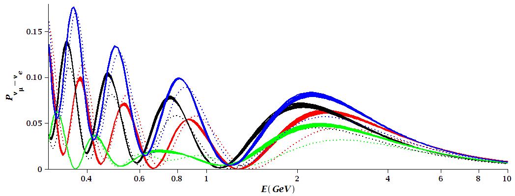
Figure 1: $\nu_{\mu}\to\nu_{e}$ oscillation probability at DUNE for normal mass hierarchy, $\delta_{cp}=0$ (red), $\delta_{cp}={\pi\over 2}$ (green), $\delta_{cp}={\pi}$ (black), $\delta_{cp}=-{\pi\over 2}$ (blue). Thickness of the plots are from varying constant/uniform matter density 2.5 - 3 g/cm³. Dotted plots are for vacuum oscillations

.

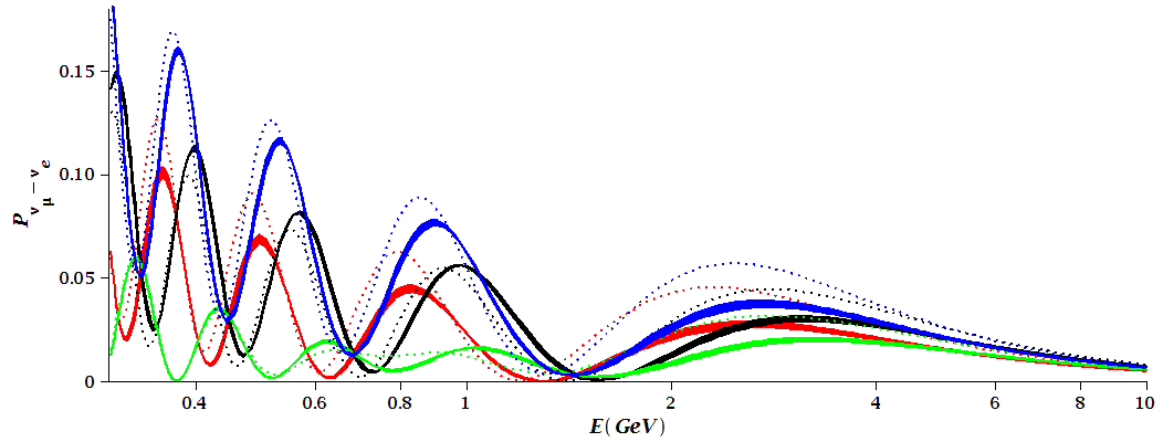
Figure 2: $\nu_{\mu}\to\nu_{e}$ oscillation probability at DUNE for inverted mass hierarchy, $\delta_{cp}=0$ (red), $\delta_{cp}={\pi\over 2}$ (green), $\delta_{cp}={\pi}$ (black), $\delta_{cp}=-{\pi\over 2}$ (blue). Thickness of the plots are from varying constant/uniform matter density 2.5 - 3 g/cm³. Dotted plots are for vacuum oscillations

.

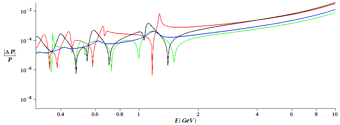
Figure 3: ${|\Delta P|\over P}\equiv{|P^{num}_{\nu_{\mu}\to\nu_{e}}-P^{anl}_{\nu_{\mu}\to\nu_{e}}|\over P^{num}_{\nu_{\mu}\to\nu_{e}}}$. The relative error of our analytic result to the exact (numeric) $\nu_{\mu}\to\nu_{e}$ oscillation probability for normal mass hierarchy, $\delta_{cp}=0$ (red), $\delta_{cp}={\pi\over 2}$ (green), $\delta_{cp}={\pi}$ (black), $\delta_{cp}=-{\pi\over 2}$ (blue). Matter density 2.6 g/cm³.

.

Appendix

In ordinary perturbation expansion in the basis of our solutions we estimate the size of effect of the neglected elements $(23),(32)$ in eq. (41).

We divide the hamiltonian into two parts

$$S=e^{-i{\cal H}L}=e^{-i{\cal H}_{0}L-i\Delta{\cal H}L}$$ (66)

Here ${\cal H}_{0}\equiv U_{m}diag(0,{\Delta m_{21}^{2}\over 2E}L,{\Delta m_{31}^{2}\over 2E}L)\ U_{m}^{\dagger}$ with our solutions for $U_{m}$ (eq 61) and mass square differences (eqs. 45 -47). $\Delta{\cal H}(23)=\Delta{\cal H}(32)=\sin\theta^{\prime}_{13}\sin 2\theta_{12}{\Delta m^{2}_{\odot}\over 4E}$ and all other elements in $\Delta{\cal H}$ are zeros. We treat $\Delta{\cal H}$ as a perturbation.

By making use well known identity $e^{a+b}=e^{a}Te^{\int_{0}^{1}dt\ e^{-a\ t}\ b\ e^{a\ t}}$ we get

$$S = S_{0}+S_{1}+\dots$$ (67)

$$S_{0} = U_{m}\left(\begin{array}[]{ccc}1&0&0\\ 0&e^{-i\phi_{21}}&0\\ 0&0&e^{-i\phi_{31}}\end{array}\right)U_{m}^{\dagger}\ \ ,\ \$$ (71)

$$S_{1} = U_{m}\left(\begin{array}[]{ccc}0&0&\cal A\\ 0&0&\cal B\\ \cal A&\cal B&0\end{array}\right)U_{m}^{\dagger}$$ (75)

where

$$\cal A = \sin\theta^{m}_{12}\ \sin\theta^{\prime}_{13}{\sin 2\theta_{12}\over 2}{\Delta m^{2}_{\odot}\over\Delta m_{31}^{2}}(1-e^{-i\phi_{31}})$$

$$\cal B = \cos\theta^{m}_{12}\ \sin\theta^{\prime}_{13}{\sin 2\theta_{12}\over 2}{\Delta m^{2}_{\odot}\over\Delta m_{31}^{2}-\Delta m_{21}^{2}}(e^{-i\phi_{31}}-e^{-i\phi_{21}})$$

$S_{0}$ is our solution for the neutrino transition matrix elements and the $S_{1}$ is its first order corrections. $|\cal A|$, $|\cal B|$ are at least smaller than 0.5% for all energies, therefore our 0^th order solution, $S_{0}$, is working excellently.

Acknowledgements. One of us (A.I.) is grateful to the CERN Theory group for its hospitality and to the DUNE members for useful discussions at Fermilab in summer 2017. A.I. is especially grateful to Pilar Coloma and Maury Goodman for underlining the importance of presenting the oscillation parameters in a simple form. S.P. is partially supported by the National Science Centre, Poland, under research grants DEC-2015/19/B/ST2/02848, DEC-2015/18/M/ST2/00054 and DEC-2014/15/B/ST2/02157.

References

• (1) L. Wolfenstein, Phys. Rev. D 17 (1978) 2369. S. P. Mikheev and A. Y. Smirnov, Sov. J. Nucl. Phys.  42 (1985) 913 [Yad. Fiz.  42 (1985) 1441].
• (2) R. Acciarri et al. [DUNE Collaboration], arXiv:1512.06148 [physics.ins-det].
• (3) S. T. Petcov, Phys. Lett. B 214 (1988) 259. doi:10.1016/0370-2693(88)91479-7 E. K. Akhmedov, R. Johansson, M. Lindner, T. Ohlsson and T. Schwetz, JHEP 0404 (2004) 078 doi:10.1088/1126-6708/2004/04/078 [hep-ph/0402175]. A. Cervera, A. Donini, M. B. Gavela, J. J. Gomez Cadenas, P. Hernandez, O. Mena and S. Rigolin, Nucl. Phys. B 579 (2000) 17 Erratum: [Nucl. Phys. B 593 (2001) 731] doi:10.1016/S0550-3213(00)00606-4, 10.1016/S0550-3213(00)00221-2 [hep-ph/0002108]. H. Nunokawa, S. J. Parke and J. W. F. Valle, Prog. Part. Nucl. Phys.  60 (2008) 338 doi:10.1016/j.ppnp.2007.10.001 [arXiv:0710.0554 [hep-ph]].
• (4) M. Blennow and A. Y. Smirnov, Adv. High Energy Phys.  2013 (2013) 972485 doi:10.1155/2013/972485 [arXiv:1306.2903 [hep-ph]].
• (5) P. B. Denton, H. Minakata and S. J. Parke, JHEP 1606 (2016) 051 doi:10.1007/JHEP06(2016)051 [arXiv:1604.08167 [hep-ph]].
• (6) P. B. Denton, H. Minakata and S. J. Parke, arXiv:1801.06514 [hep-ph].
• (7) P. I. Krastev and S. T. Petcov, Phys. Lett. B 205 (1988) 84. doi:10.1016/0370-2693(88)90404-2
• (8) O. L. G. Peres and A. Y. Smirnov, Nucl. Phys. B 680 (2004) 479 doi:10.1016/j.nuclphysb.2003.12.017 [hep-ph/0309312].
• (9) C. Patrignani et al. [Particle Data Group], Chin. Phys. C 40 (2016) no.10, 100001. doi:10.1088/1674-1137/40/10/100001
• (10) H. Nunokawa, S. J. Parke and R. Zukanovich Funchal, Phys. Rev. D 72 (2005) 013009 doi:10.1103/PhysRevD.72.013009 [hep-ph/0503283].