A mathematical solve on the three-interfering-resonances’ parameters

Abstract

The multiple-solution problem in determining the three-interfering-resonances’ parameters from a fit to an experimentally measured distribution is considered in a mathematical viewpoint. In this paper it is shown that there are four numerical solutions for the fit with three coherent Breit-Wigner functions. Although the explicit analytical formulae can not be derived in this case, we provide some constraint equations between the four solutions. For the cases of nonrelativistic and relativistic Breit-Wigner forms of amplitude functions, numerical method is provided to derive the other solutions from the already obtained one based on the obtained constraint equations. In real experimental measurements with more complicated amplitude forms similar to Breit-Wigner functions, the same method can be deduced and performed to get numerical solutions. The well agreement between the solved solutions using this mathematical method and those from the fit directly verifies the correctness of the supplied constraint equations and mathematical methodology.

I Introduction

One of the main aims during the physics analysis of experimental data is determination of the parameters of several resonances by fitting the cross sections or measured mass spectrum with possible interference between the resonances considered. In some cases, although the fitted results with interference are not taken as nominal results, the interference still needs to be considered as an estimate of the systematic uncertainty.

In particle physics, we usually take Breit-Wigner (BW) function to represent resonance amplitude. And a typical task is determination of the BW parameters from the fit to the measured distributions in experiment, such as cross sections. The measured physical quantities are usually in proportion to the modulus of the total amplitude squared, for examples, $|BW_{1}+BW_{2}e^{i\phi}|^{2}$ for two interfering resonances and $|BW_{1}+BW_{2}e^{i\phi_{1}}+BW_{3}e^{i\phi_{2}|^{2}}$ for three interfering resonances, where $\phi$, $\phi_{1}$, and $\phi_{2}$ are the relative phases between resonances. Due to this square operation in the amplitudes to connect with the measured physical quantities, we could find multi-solutions in extracting amplitudes from the fit to the experimental measurements. Often it occurs that these multi-solutions have the same goodness-of-the-fit, and resonance mass and width, but relative phases are different. This indicates that different solutions have different coupling strength to decay channels, which would result in different interpretations in physics. Therefore for the fit with interfering resonances, we need to make sure that all the solutions have been found. If there are multiple solutions, but only one is reported, the experimental results may be incomplete or even biased.

Recently, more and more experimental analyses, especially the studies of the vector charmonium-like $Y$ states, have indicated this. For example, in Ref. wang two or three coherent resonances plus an incoherent background shape are used to fit the $\pi^{+}\pi^{-}\psi(2S)$ invariant mass distribution. Correspondingly two or four solutions are found with identical resonance mass and width but different couplings to electron-positron pairs. Another example is presented in Ref. yuan2010multiple , where two solutions are found in the branching fraction measurement for $\phi\to\omega\pi^{0}$ process and the study of $\rho-\omega$ mixing.

In real physics analyses, all the multiple solutions are found via fitting process. Due to the background statistical fluctuation or limited statistics, not all the solutions can be found easily in some cases. Therefore, from the mathematical point of view, a nature question is raised: if a particular solution has been found, then whether other solutions can be derived from it. For the above question, the authors in Refs. zhu2011mathematical ; bukin proved that if we use two coherent BW functions to fit the measured distribution, there should be only two different solutions, and they can be derived each other by using analytical formulae and a numerical method. As pointed out in Ref. bukin , in the case of three resonances with constant widths there occurred four solutions with the same likelihood function minimum, but analytical solution of this problem appeared too hard due to technical difficulties.

In this paper, we discuss the multiple-solution problem in determining the resonant parameters of three interfering resonances in a mathematical viewpoint. Although the explicit analytical formulae can not be derived, we provide some constraint equations between four solutions. We also provide a mathematical method to get additional solutions from the obtained one.

This work is organized as follows. After the Introduction, we present a general mathematic model for the amplitudes of three coherent resonance states in Sec. II. If three resonances are described by the normal BW functions, the analytical expressions for the relationship between the four solutions are deduced and obtained. An effective approach is developed to obtain the algebra equations of the relationship between the four solutions. In Sec. III, the relations between the four solutions are also deduced for relativistic BW forms. In Sec. IV, two numerical examples produced by toy Monte Carlo (MC) are utilized to cross check and confirm our results. When the form of resonance amplitude is extremely complex, we can take a similar numerical procedure to obtain other unknown solutions from the known one. Finally, in Sec. V, a short discussion is given.

II Mathematical methodology for three simple-BW-amplitudes case

In the light of two distinct features: (1) all solutions have the same goodness-of-fit; (2) different solutions have identical resonance mass and width but different couplings to electron-positron pairs, we construct a general mathematical model for multiple solutions based on three interfering amplitude functions.

A sum of three quantum amplitudes can be described by a complex function $e(x,z_{1},z_{2},z_{3})$ with form

$$e(x,z_{1},z_{2},z_{3})=z_{1}\ g(x)+z_{2}\ f(x)+z_{3}\ h(x)~{},$$ (1)

where $x$ is a measured variable, $g(x)$, $h(x)$, and $f(x)$ are complex functions of $x$, and $z_{1}$, $z_{2}$, and $z_{3}$ are complex numbers. Our purpose is to find different parameters $z^{\prime}_{1}$, $z^{\prime}_{2}$, and $z^{\prime}_{3}$ satisfying

$$\left|e(x,z_{1},z_{2},z_{3})\right|^{2}=\left|e(x,z^{\prime}_{1},z^{\prime}_{2},z^{\prime}_{3})\right|^{2}~{}.$$ (2)

Since the global phase does not work on amplitude squared operation we can reduce the dimension of $\{z_{1},z_{2},z_{3}\}$ parameter space to a $\{d,z_{\alpha},z_{\beta}\}$ parameter space, where $d$ is a real number. The module of the amplitude squared of $e(x,z_{1},z_{2},z_{3})$, $\left|e(x,z_{1},z_{2},z_{3})\right|^{2}$, can be rewritten in a more convenient form by defining

$$\left|e(x,z_{1},z_{2},z_{3})\right|^{2}\equiv\frac{1}{d}\left|g(x)+z_{\alpha}f(x)+z_{\beta}h(x)\right|^{2}=\frac{\left|g(x)\right|^{2}}{d}\left|1+z_{\alpha}\frac{f(x)}{g(x)}+z_{\beta}\frac{h(x)}{g(x)}\right|^{2}$$ (3)

$$\equiv\frac{\left|g(x)\right|^{2}}{d}\left|1+z_{\alpha}F(x)+z_{\beta}H(x)\right|^{2}\equiv\frac{\left|g(x)\right|^{2}}{d}E(x,z_{\alpha},z_{\beta})~{}.$$ (4)

Here $F(x)\equiv f(x)/g(x)$, $H(x)\equiv h(x)/g(x)$. Considering $\left|g(x)\right|^{2}$ is only a product factor and is independent of $z_{\alpha}$, $z_{\beta}$, and $d$, we remove it in the following derivation. What we need to do now is to find different $z_{\alpha}$, $z_{\beta}$, and $d$ values which keep $E(x,z_{\alpha},z_{\beta})/d$ unchanged.

Taking ($R_{F}(x)$, $I_{F}(x)$), ($R_{H}(x)$, $I_{H}(x)$), ($R_{z_{\alpha}}$, $I_{z_{\alpha}}$), and ($R_{z_{\beta}}$, $I_{z_{\beta}}$) as real and imaginary parts of $F(x)$, $H(x)$, $z_{\alpha}$, and $z_{\beta}$, respectively, and using them to represent $E(x,z_{\alpha},z_{\beta})$, we get

$$E(x,z_{\alpha},z_{\beta})=1 +(R_{F}^{2}+I_{F}^{2})(R_{z_{\alpha}}^{2}+I_{z_{\alpha}}^{2})+2R_{z_{\alpha}}R_{F}-2I_{z_{\alpha}}I_{F}$$

$$+(R_{H}^{2}+I_{H}^{2})(R_{z_{\beta}}^{2}+I_{z_{\beta}}^{2})+2R_{z_{\beta}}R_{H}-2I_{z_{\beta}}I_{H}$$

$$+2(R_{F}R_{H}+I_{F}I_{H})(R_{z_{\alpha}}R_{z_{\beta}}+I_{z_{\alpha}}I_{z_{\beta}})$$

$$-2(R_{F}I_{H}-I_{F}R_{H})(R_{z_{\alpha}}I_{z_{\beta}}-I_{z_{\alpha}}R_{z_{\beta}}).$$ (5)

For the sake of brevity, the specific form of dependence of $R_{F}(x)$, $I_{F}(x)$, $R_{H}(x)$, and $I_{H}(x)$ on $x$ is removed here. Without loss of generality, we take $d=1$ as an initial solution for convenience. The next task is to find all the possible $z_{\alpha}^{\prime}$, $z_{\beta}^{\prime}$, and $d^{\prime}$ values to make $E(x,z_{\alpha}^{\prime},z_{\beta}^{\prime})/d^{\prime}=E(x,z_{\alpha},z_{\beta})$. To be more specific about our work, we consider that $g(x)$, $h(x)$, and $f(x)$ are widely accepted nonrelativistic BW functions as an example.

$$g(x)=\frac{\Gamma_{g}}{(x-M_{g})+i\Gamma_{g}},~{}~{}~{}~{}f(x)=\frac{\Gamma_{f}}{(x-M_{f})+i\Gamma_{f}},~{}~{}~{}~{}h(x)=\frac{\Gamma_{h}}{(x-M_{h})+i\Gamma_{h}},$$ (6)

where $M$ is the mass and $\Gamma$ is the width for a resonance, respectively. Using the above forms of $g(x)$, $h(x)$, and $f(x)$, the real and imaginary parts of $F(x)$ and $H(x)$ become

$$R_{F}=\frac{\Gamma_{f}[\Gamma_{g}\Gamma_{f}+(M_{g}-x)(M_{f}-x)]}{\Gamma_{g}[\Gamma_{f}^{2}+(M_{f}-x)^{2}]},~{}~{}~{}I_{F}=\frac{\Gamma_{f}[\Gamma_{f}(M_{g}-x)-\Gamma_{g}(M_{f}-x)]}{\Gamma_{g}[\Gamma_{f}^{2}+(M_{f}-x)^{2}]},$$

$$R_{H}=\frac{\Gamma_{h}[\Gamma_{g}\Gamma_{h}+(M_{g}-x)(M_{h}-x)]}{\Gamma_{g}[\Gamma_{h}^{2}+(M_{h}-x)^{2}]},~{}~{}~{}I_{H}=\frac{\Gamma_{h}[\Gamma_{h}(M_{g}-x)-\Gamma_{g}(M_{h}-x)]}{\Gamma_{g}[\Gamma_{h}^{2}+(M_{h}-x)^{2}]},$$

respectively. After some algebra, we obtain the interesting relations below:

$$R_{F}^{2}+I_{F}^{2}=a_{f}R_{F}+b_{f}I_{F}+c_{f},~{}~{}~{}R_{H}^{2}+I_{H}^{2}=a_{h}R_{H}+b_{h}I_{H}+c_{h},$$ (7)

with

$$a_{f}=\frac{\Gamma_{g}+\Gamma_{f}}{\Gamma_{g}}\;,\;\;b_{f}=\frac{M_{g}-M_{f}}{\Gamma_{g}}\;,\;\;c_{f}=-\frac{\Gamma_{f}}{\Gamma_{g}}\;,\;\;$$ (8)

$$a_{h}=\frac{\Gamma_{g}+\Gamma_{h}}{\Gamma_{g}}\;,\;\;b_{h}=\frac{M_{g}-M_{h}}{\Gamma_{g}}\;,\;\;c_{h}=-\frac{\Gamma_{h}}{\Gamma_{g}}\;.\;\;$$ (9)

With Eq. (7), $E(x,z_{\alpha},z_{\beta})$ is recast as

$$E(x,z_{\alpha},z_{\beta})=~{} R_{F}(a_{f}R_{z_{\alpha}}^{2}+a_{f}I_{z_{\alpha}}^{2}+2R_{z_{\alpha}})+I_{F}(b_{f}R_{z_{\alpha}}^{2}+b_{f}I_{z_{\alpha}}^{2}-2I_{z_{\alpha}})$$

$$+ R_{H}(a_{h}R_{z_{\beta}}^{2}+a_{h}I_{z_{\beta}}^{2}+2R_{z_{\beta}})+I_{H}(b_{h}R_{z_{\beta}}^{2}+b_{h}I_{z_{\beta}}^{2}-2I_{z_{\beta}})$$

$$+ 2\ (R_{F}R_{H}+I_{F}I_{H})(R_{z_{\alpha}}R_{z_{\beta}}+I_{z_{\alpha}}I_{z_{\beta}})$$ (10)

$$- 2\ (R_{F}I_{H}-I_{F}R_{H})(R_{z_{\alpha}}I_{z_{\beta}}-I_{z_{\alpha}}R_{z_{\beta}})$$

$$+ c_{f}(R_{z_{\alpha}}^{2}+I_{z_{\alpha}}^{2})+c_{h}(R_{z_{\beta}}^{2}+I_{z_{\beta}}^{2})+1.$$

Similar expression can be obtained for $E(x,z_{\alpha}^{\prime},z_{\beta}^{\prime})$. Notice that $R_{F}$, $I_{F}$, $R_{H}$, and $I_{H}$ are functions in variable space (namely $x$ space), and $[c_{f}(R_{z_{\alpha}}^{2}+I_{z_{\alpha}}^{2})+c_{h}(R_{z_{\beta}}^{2}+I_{z_{\beta}}^{2})+1]$ is a constant for $x$ space. We noticed that the term $(R_{F}R_{H}+I_{F}I_{H})$ and the linear combination of $R_{F}$, $I_{F}$, $R_{H}$, and $I_{H}$ have the same number of $x$ terms with the same power. It is the same for the term $(R_{F}I_{H}-I_{F}R_{H})$. So there are linear correlations for $(R_{F}R_{H}+I_{F}I_{H})$ and $(R_{F}I_{H}-I_{F}R_{H})$ by factors $\{c_{1},c_{2},c_{3},c_{4},c_{5}\}$ and $\{c_{6},c_{7},c_{8},c_{9},c_{10}\}$, respectively. That means $(R_{F}R_{H}+I_{F}I_{H})$ and $(R_{F}I_{H}-I_{F}R_{H})$ can be represented by $R_{F}$, $I_{F}$, $R_{H}$, $I_{H}$, and a constant term.

$$R_{F}R_{H}+I_{F}I_{H}=c_{1}R_{F}+c_{2}I_{F}+c_{3}R_{H}+c_{4}I_{H}+c_{5}[c_{f}(R_{z_{\alpha}}^{2}+I_{z_{\alpha}}^{2})+c_{h}(R_{z_{\beta}}^{2}+I_{z_{\beta}}^{2})+1],$$ (11)

$$R_{F}I_{H}-I_{F}R_{H}=c_{6}R_{F}+c_{7}I_{F}+c_{8}R_{H}+c_{9}I_{H}+c_{10}[c_{f}(R_{z_{\alpha}}^{2}+I_{z_{\alpha}}^{2})+c_{h}(R_{z_{\beta}}^{2}+I_{z_{\beta}}^{2})+1].$$

The factors $\{c_{1},c_{2},c_{3},c_{4},c_{5}\}$ and $\{c_{6},c_{7},c_{8},c_{9},c_{10}\}$ follow Eq. (II):

$$c_{1}= \frac{\Gamma_{h}(M_{f}^{2}+M_{g}M_{h}-M_{f}(M_{g}+M_{h})+(\Gamma_{f}+\Gamma_{g})(\Gamma_{f}+\Gamma_{h}))}{\Gamma_{g}(M_{f}^{2}-2M_{f}M_{h}+M_{h}^{2}+(\Gamma_{f}+\Gamma_{h})^{2})},$$

$$c_{2}= \frac{\Gamma_{h}(-M_{h}(\Gamma_{f}+\Gamma_{g})+M_{f}(\Gamma_{g}-\Gamma_{h})+M_{g}(\Gamma_{f}+\Gamma_{h}))}{\Gamma_{g}(M_{f}^{2}-2M_{f}M_{h}+M_{h}^{2}+(\Gamma_{f}+\Gamma_{h})^{2})},$$

$$c_{3}= \frac{\Gamma_{f}(M_{f}(M_{g}-M_{h})-M_{g}M_{h}+M_{h}^{2}+\Gamma_{f}\Gamma_{g}+\Gamma_{f}\Gamma_{h}+\Gamma_{g}\Gamma_{h}+\Gamma_{h}^{2})}{\Gamma_{g}(M_{f}^{2}-2M_{f}M_{h}+M_{h}^{2}+(\Gamma_{f}+\Gamma_{h})^{2})},$$

$$c_{4}= \frac{\Gamma_{f}(M_{h}(-\Gamma_{f}+\Gamma_{g})+M_{g}(\Gamma_{f}+\Gamma_{h})-M_{f}(\Gamma_{g}+\Gamma_{h}))}{\Gamma_{g}(M_{f}^{2}-2M_{f}M_{h}+M_{h}^{2}+(\Gamma_{f}+\Gamma_{h})^{2})},$$

$$c_{5}= -\frac{2\Gamma_{f}\Gamma_{h}(\Gamma_{f}+\Gamma_{h})}{\Gamma_{g}(M_{f}^{2}-2M_{f}M_{h}+M_{h}^{2}+(\Gamma_{f}+\Gamma_{h})^{2})},$$ (12)

$$c_{6}= \frac{\Gamma_{h}(-M_{h}(\Gamma_{f}+\Gamma_{g})+M_{f}(\Gamma_{g}-\Gamma_{h})+M_{g}(\Gamma_{f}+\Gamma_{h}))}{\Gamma_{g}(M_{f}^{2}-2M_{f}M_{h}+M_{h}^{2}+(\Gamma_{f}+\Gamma_{h})^{2})},$$

$$c_{7}= -\frac{\Gamma_{h}(M_{f}^{2}+M_{g}M_{h}-M_{f}(M_{g}+M_{h})+(\Gamma_{f}+\Gamma_{g})(\Gamma_{f}+\Gamma_{h}))}{\Gamma_{g}(M_{f}^{2}-2M_{f}M_{h}+M_{h}^{2}+(\Gamma_{f}+\Gamma_{h})^{2})},$$

$$c_{8}= \frac{\Gamma_{f}(M_{h}(\Gamma_{f}-\Gamma_{g})-M_{g}(\Gamma_{f}+\Gamma_{h})+M_{f}(\Gamma_{g}+\Gamma_{h}))}{\Gamma_{g}(M_{f}^{2}-2M_{f}M_{h}+M_{h}^{2}+(\Gamma_{f}+\Gamma_{h})^{2})},$$

$$c_{9}= \frac{\Gamma_{f}(M_{f}(M_{g}-M_{h})-M_{g}M_{h}+M_{h}^{2}+\Gamma_{f}\Gamma_{g}+\Gamma_{f}\Gamma_{h}+\Gamma_{g}\Gamma_{h}+\Gamma_{h}^{2})}{\Gamma_{g}(M_{f}^{2}-2M_{f}M_{h}+M_{h}^{2}+(\Gamma_{f}+\Gamma_{h})^{2})},$$

$$c_{10}= \frac{2(-M_{f}+M_{h})\Gamma_{f}\Gamma_{h}}{\Gamma_{g}(M_{f}^{2}-2M_{f}M_{h}+M_{h}^{2}+(\Gamma_{f}+\Gamma_{h})^{2})}.$$

Then we can get

$$E(x,z_{\alpha},z_{\beta})=~{} R_{F}(a_{f}R_{z_{\alpha}}^{2}+a_{f}I_{z_{\alpha}}^{2}+2R_{z_{\alpha}}+c_{1}A+c_{6}B)+I_{F}(b_{f}R_{z_{\alpha}}^{2}+b_{f}I_{z_{\alpha}}^{2}-2I_{z_{\alpha}}+c_{2}A+c_{7}B)$$

$$+ R_{H}(a_{h}R_{z_{\beta}}^{2}+a_{h}I_{z_{\beta}}^{2}+2R_{z_{\beta}}+c_{3}A+c_{8}B)+I_{H}(b_{h}R_{z_{\beta}}^{2}+b_{h}I_{z_{\beta}}^{2}-2I_{z_{\beta}}+c_{4}A+c_{9}B)$$

$$+ c_{f}R_{z_{\alpha}}^{2}+c_{f}I_{z_{\alpha}}^{2}+c_{h}R_{z_{\beta}}^{2}+c_{h}I_{z_{\beta}}^{2}+1+c_{5}A+c_{10}B,$$ (13)

with $A=2(R_{z_{\alpha}}R_{z_{\beta}}+I_{z_{\alpha}}I_{z_{\beta}})$ and $B=-2(R_{z_{\alpha}}I_{z_{\beta}}-I_{z_{\alpha}}R_{z_{\beta}})$.

We know that $R_{z_{\alpha}}$, $I_{z_{\alpha}}$, $R_{z_{\beta}}$, and $I_{z_{\beta}}$ are functions in parameter space $\{d,z_{\alpha},z_{\beta}\}$. If we want to make $E(x,z_{\alpha}^{\prime},z_{\beta}^{\prime})/d^{\prime}=E(x,z_{\alpha},z_{\beta})$ hold for any $x$, then the corresponding coefficients of the functions in parameter space should be equal, which immediately leads to the following equations:

$$\frac{1}{d^{\prime}}(a_{f}R_{z_{\alpha}}^{\prime 2}+a_{f}I_{z_{\alpha}}^{\prime 2}+2R_{z_{\alpha}}^{\prime}+c_{1}A^{\prime}+c_{6}B^{\prime}) =a_{f}R_{z_{\alpha}}^{2}+a_{f}I_{z_{\alpha}}^{2}+2R_{z_{\alpha}}+c_{1}A+c_{6}B,$$

$$\frac{1}{d^{\prime}}(b_{f}R_{z_{\alpha}}^{\prime 2}+b_{f}I_{z_{\alpha}}^{\prime 2}-2I_{z_{\alpha}}^{\prime}+c_{2}A^{\prime}+c_{7}B^{\prime}) =b_{f}R_{z_{\alpha}}^{2}+b_{f}I_{z_{\alpha}}^{2}-2I_{z_{\alpha}}+c_{2}A+c_{7}B,$$

$$\frac{1}{d^{\prime}}(a_{h}R_{z_{\beta}}^{\prime 2}+a_{h}I_{z_{\beta}}^{\prime 2}+2R_{z_{\beta}}^{\prime}+c_{3}A^{\prime}+c_{8}B^{\prime}) =a_{h}R_{z_{\beta}}^{2}+a_{h}I_{z_{\beta}}^{2}+2R_{z_{\beta}}+c_{3}A+c_{8}B,$$ (14)

$$\frac{1}{d^{\prime}}(b_{h}R_{z_{\beta}}^{\prime 2}+b_{h}I_{z_{\beta}}^{\prime 2}-2I_{z_{\beta}}^{\prime}+c_{4}A^{\prime}+c_{9}B^{\prime}) =b_{h}R_{z_{\beta}}^{2}+b_{h}I_{z_{\beta}}^{2}-2I_{z_{\beta}}+c_{4}A+c_{9}B,$$

$$\frac{1}{d^{\prime}}(c_{f}R_{z_{\alpha}}^{\prime 2}+c_{f}I_{z_{\alpha}}^{\prime 2}+c_{h}R_{z_{\beta}}^{\prime 2}+c_{h}I_{z_{\beta}}^{\prime 2}+1+c_{5}A^{\prime}+c_{10}B^{\prime}) =c_{f}R_{z_{\alpha}}^{2}+c_{f}I_{z_{\alpha}}^{2}+c_{h}R_{z_{\beta}}^{2}+c_{h}I_{z_{\beta}}^{2}+1+c_{5}A+c_{10}B,$$

with

$$A^{\prime}=2(R_{z_{\alpha}}^{\prime}R_{z_{\beta}}^{\prime}+I_{z_{\alpha}}^{\prime}I_{z_{\beta}}^{\prime}), A=2(R_{z_{\alpha}}R_{z_{\beta}}+I_{z_{\alpha}}I_{z_{\beta}}),$$

$$B^{\prime}=-2(R_{z_{\alpha}}^{\prime}I_{z_{\beta}}^{\prime}-I_{z_{\alpha}}^{\prime}R_{z_{\beta}}^{\prime}), B=-2(R_{z_{\alpha}}I_{z_{\beta}}-I_{z_{\alpha}}R_{z_{\beta}}).$$

All what we need is to solve the Eq. (II) to obtain the values of $R_{z_{\alpha}}^{\prime}$, $I_{z_{\alpha}}^{\prime}$, $R_{z_{\beta}}^{\prime}$, $I_{z_{\beta}}^{\prime}$, and $d^{\prime}$. Unfortunately, there are no explicit analytical expressions for them. So we can not prove there must be four solutions. Such conclusion agrees with that in Ref. bukin . However, by using mathematica tool mathe to input Eq. (II) and initial solution, we exactly get four numerical solutions quickly. The numerical solutions can be taken as cross checks and references compared with those from the fits. This definitely saves a lot of time and energy.

We need to point out that the Eqs. (7), (11), (II), and (II) are independent on the explicit expressions of BW functions, while the factors such as $a_{f}$, $b_{f}$, $c_{f}$, $a_{h}$, $b_{h}$, $c_{h}$, $\{c_{1},c_{2},c_{3},c_{4},c_{5}\}$, and $\{c_{6},c_{7},c_{8},c_{9},c_{10}\}$ are dependent.

III Mathematical Methodology for three relativistic-BW-amplitudes case

Here we take another form for $f(x)$ , $g(x)$, and $h(x)$, i.e., relativistic BW amplitudes that are usually used in $e^{+}e^{-}$ reactions to extract the parameters of $Y$ resonance:

$$BW(s)=\frac{\sqrt{12\pi\Gamma_{e^{+}e^{-}}^{R}{\cal B}_{R}\Gamma_{R}}}{s-M^{2}_{R}+iM_{R}\Gamma_{R}}\sqrt{\frac{PS(\sqrt{s})}{PS(M_{R})}},$$ (15)

where $s$ is the $e^{+}e^{-}$ center-of-mass square; $M_{R}$ is the mass of the resonance $R$; $\Gamma_{R}$ and $\Gamma_{e^{+}e^{-}}^{R}$ are the total width and partial width to $e^{+}e^{-}$, respectively; ${\cal B}_{R}$ is the branching fraction of the resonance $R$ decays into a final state; and $PS$ is the $n-$body decay phase space factor which increases smoothly from the mass threshold with the $\sqrt{s}$ pdg . Notice that the Eq. (II) is independent on the forms of amplitudes, while its coefficients will change. With some algebra, we can obtain the coefficients for other forms of amplitudes.

With Eq. (15), the $F(x)$ and $H(x)$ are changed to

$$F(x)=\frac{x^{2}-M_{g}^{2}+iM_{g}\Gamma_{g}}{x^{2}-M_{f}^{2}+iM_{f}\Gamma_{f}}\sqrt{\frac{\Gamma_{f}PS(M_{g})}{\Gamma_{g}PS(M_{f})}},$$

$$H(x)=\frac{x^{2}-M_{g}^{2}+iM_{g}\Gamma_{g}}{x^{2}-M_{h}^{2}+iM_{h}\Gamma_{h}}\sqrt{\frac{\Gamma_{h}PS(M_{g})}{\Gamma_{g}PS(M_{h})}}.$$

In this situation, $R_{F}$, $I_{F}$, $R_{H}$, and $I_{H}$ are changed. So we need resolve the parameters $a_{f}$, $b_{f}$, $c_{f}$, $a_{h}$, $b_{h}$, $c_{h}$, $\{c_{1},c_{2},c_{3},c_{4},c_{5}\}$, and $\{c_{6},c_{7},c_{8},c_{9},c_{10}\}$ using Eqs. (7) and (11), respectively. And we obtain

$$a_{f}=\frac{(\Gamma_{f}M_{f}+\Gamma_{g}M_{g})}{M_{f}\sqrt{\Gamma_{f}\Gamma_{g}}}\sqrt{\frac{PS(M_{g})}{PS(M_{f})}},\;\;b_{f}=-\frac{(M_{f}^{2}-M_{g}^{2})}{M_{f}\sqrt{\Gamma_{f}\Gamma_{g}}}\sqrt{\frac{PS(M_{g})}{PS(M_{f})}}\;,\;\;c_{f}=-\frac{M_{g}PS(M_{g})}{M_{f}PS(M_{f})}\;,\;$$ (16)

$$a_{h}=\frac{(\Gamma_{h}M_{h}+\Gamma_{g}M_{g})}{M_{h}\sqrt{\Gamma_{h}\Gamma_{g}}}\sqrt{\frac{PS(M_{g})}{PS(M_{h})}}\;,\;\;b_{h}=-\frac{(M_{h}^{2}-M_{g}^{2})}{M_{h}\sqrt{\Gamma_{h}\Gamma_{g}}}\sqrt{\frac{PS(M_{g})}{PS(M_{h})}}\;,\;\;c_{h}=-\frac{M_{g}PS(M_{g})}{M_{h}PS(M_{h})}\;,\;\;$$ (17)

and

$$c_{1}= \frac{\sqrt{\Gamma_{h}PS(g)}\left[M_{f}^{4}-M_{f}^{2}\left(-\Gamma_{f}^{2}+M_{g}^{2}+M_{h}^{2}\right)+\Gamma_{f}M_{f}(\Gamma_{g}M_{g}+\Gamma_{h}M_{h})+M_{g}M_{h}(\Gamma_{g}\Gamma_{h}+M_{g}M_{h})\right]}{\sqrt{\Gamma_{g}PS(h)}\left[M_{f}^{4}+M_{f}^{2}\left(\Gamma_{f}^{2}-2M_{h}^{2}\right)+2\Gamma_{f}\Gamma_{h}M_{f}M_{h}+M_{h}^{2}\left(\Gamma_{h}^{2}+M_{h}^{2}\right)\right]},$$

$$c_{2}= -\frac{\sqrt{\Gamma_{h}PS(g)}\left[M_{f}^{2}(\Gamma_{h}M_{h}-\Gamma_{g}M_{g})+\Gamma_{f}M_{f}\left(M_{h}^{2}-M_{g}^{2}\right)+M_{g}M_{h}(\Gamma_{g}M_{h}-\Gamma_{h}M_{g})\right]}{\sqrt{\Gamma_{g}PS(h)}\left[M_{f}^{4}+M_{f}^{2}\left(\Gamma_{f}^{2}-2M_{h}^{2}\right)+2\Gamma_{f}\Gamma_{h}M_{f}M_{h}+M_{h}^{2}\left(\Gamma_{h}^{2}+M_{h}^{2}\right)\right]},$$

$$c_{3}= \frac{\sqrt{\Gamma_{f}PS(g)}\left[M_{f}^{2}\left(M_{g}^{2}-M_{h}^{2}\right)+\Gamma_{f}M_{f}(\Gamma_{g}M_{g}+\Gamma_{h}M_{h})+M_{h}\left(-M_{g}^{2}M_{h}+\Gamma_{g}\Gamma_{h}M_{g}+M_{h}^{3}+\Gamma_{h}^{2}M_{h}\right)\right]}{\sqrt{\Gamma_{g}PS(f)}\left[M_{f}^{4}+M_{f}^{2}\left(\Gamma_{f}^{2}-2M_{h}^{2}\right)+2\Gamma_{f}\Gamma_{h}M_{f}M_{h}+M_{h}^{2}\left(\Gamma_{h}^{2}+M_{h}^{2}\right)\right]},$$

$$c_{4}= \frac{\sqrt{\Gamma_{f}PS(g)}\left[M_{f}^{2}(-(\Gamma_{g}M_{g}+\Gamma_{h}M_{h}))+\Gamma_{f}M_{f}\left(M_{g}^{2}-M_{h}^{2}\right)+M_{g}M_{h}(\Gamma_{h}M_{g}+\Gamma_{g}M_{h})\right]}{\sqrt{\Gamma_{g}PS(f)}\left[M_{f}^{4}+M_{f}^{2}\left(\Gamma_{f}^{2}-2M_{h}^{2}\right)+2\Gamma_{f}\Gamma_{h}M_{f}M_{h}+M_{h}^{2}\left(\Gamma_{h}^{2}+M_{h}^{2}\right)\right]},$$

$$c_{5}= -\frac{2M_{g}PS(g)\sqrt{\Gamma_{f}\Gamma_{h}}(\Gamma_{f}M_{f}+\Gamma_{h}M_{h})}{\sqrt{PS(f)PS(h)}\left[M_{f}^{4}+M_{f}^{2}\left(\Gamma_{f}^{2}-2M_{h}^{2}\right)+2\Gamma_{f}\Gamma_{h}M_{f}M_{h}+M_{h}^{2}\left(\Gamma_{h}^{2}+M_{h}^{2}\right)\right]},$$ (18)

$$c_{6}= -\frac{\sqrt{\Gamma_{h}PS(g)}\left[M_{f}^{2}(\Gamma_{h}M_{h}-\Gamma_{g}M_{g})+\Gamma_{f}M_{f}\left(M_{h}^{2}-M_{g}^{2}\right)+M_{g}M_{h}(\Gamma_{g}M_{h}-\Gamma_{h}M_{g})\right]}{\sqrt{\Gamma_{g}PS(h)}\left[M_{f}^{4}+M_{f}^{2}\left(\Gamma_{f}^{2}-2M_{h}^{2}\right)+2\Gamma_{f}\Gamma_{h}M_{f}M_{h}+M_{h}^{2}\left(\Gamma_{h}^{2}+M_{h}^{2}\right)\right]},$$

$$c_{7}= -\frac{\sqrt{\Gamma_{h}PS(g)}\left[M_{f}^{4}-M_{f}^{2}\left(-\Gamma_{f}^{2}+M_{g}^{2}+M_{h}^{2}\right)+\Gamma_{f}M_{f}(\Gamma_{g}M_{g}+\Gamma_{h}M_{h})+M_{g}M_{h}(\Gamma_{g}\Gamma_{h}+M_{g}M_{h})\right]}{\sqrt{\Gamma_{g}PS(h)}\left[M_{f}^{4}+M_{f}^{2}\left(\Gamma_{f}^{2}-2M_{h}^{2}\right)+2\Gamma_{f}\Gamma_{h}M_{f}M_{h}+M_{h}^{2}\left(\Gamma_{h}^{2}+M_{h}^{2}\right)\right]},$$

$$c_{8}= -\frac{\sqrt{\Gamma_{f}PS(g)}\left[M_{f}^{2}(-(\Gamma_{g}M_{g}+\Gamma_{h}M_{h}))+\Gamma_{f}M_{f}\left(M_{g}^{2}-M_{h}^{2}\right)+M_{g}M_{h}(\Gamma_{h}M_{g}+\Gamma_{g}M_{h})\right]}{\sqrt{\Gamma_{g}PS(f)}\left[M_{f}^{4}+M_{f}^{2}\left(\Gamma_{f}^{2}-2M_{h}^{2}\right)+2\Gamma_{f}\Gamma_{h}M_{f}M_{h}+M_{h}^{2}\left(\Gamma_{h}^{2}+M_{h}^{2}\right)\right]},$$

$$c_{9}= \frac{\sqrt{\Gamma_{f}PS(g)}\left[M_{f}^{2}\left(M_{g}^{2}-M_{h}^{2}\right)+\Gamma_{f}M_{f}(\Gamma_{g}M_{g}+\Gamma_{h}M_{h})+M_{h}\left(-M_{g}^{2}M_{h}+\Gamma_{g}\Gamma_{h}M_{g}+M_{h}^{3}+\Gamma_{h}^{2}M_{h}\right)\right]}{\sqrt{\Gamma_{g}PS(f)}\left[M_{f}^{4}+M_{f}^{2}\left(\Gamma_{f}^{2}-2M_{h}^{2}\right)+2\Gamma_{f}\Gamma_{h}M_{f}M_{h}+M_{h}^{2}\left(\Gamma_{h}^{2}+M_{h}^{2}\right)\right]},$$

$$c_{10}= -\frac{2M_{g}PS(g)\sqrt{\Gamma_{f}\Gamma_{h}}\left(M_{f}^{2}-M_{h}^{2}\right)}{\sqrt{PS(f)PS(h)}\left[M_{f}^{4}+M_{f}^{2}\left(\Gamma_{f}^{2}-2M_{h}^{2}\right)+2\Gamma_{f}\Gamma_{h}M_{f}M_{h}+M_{h}^{2}\left(\Gamma_{h}^{2}+M_{h}^{2}\right)\right]}.$$

Substitute the above factors into Eq. (II), the relationship between multi-solutions can be obtained, therefore, one can derive the other three solutions from the already obtained one mathe .

IV Check and Application

IV.1 Simple BW amplitudes

In order to verify our deduction on constraint equations and mathematical program in obtaining numerical solutions, let us take a random example for the case of three simple BW amplitudes with interference. The parameter values of the three BW functions as one solution are set as

$$M_{g}=3.80,\;\;\Gamma_{g}=0.03,$$

$$M_{f}=4.00,\;\;\Gamma_{f}=0.04,\;\;\phi_{f}=\pi/3,$$

$$M_{h}=4.25,\;\;\Gamma_{h}=0.06,\;\;\phi_{h}=3\pi/4.$$

The module of the amplitude squared of three interfering resonances is $\left|BW_{g}(m)+BW_{f}(m)e^{i\phi_{f}}+BW_{h}(m)e^{i\phi_{h}}\right|^{2}$ and the BW amplitudes use the formats shown in Eq. (6). That is to say $z_{\alpha}=e^{i\phi_{f}}=1/2+\sqrt{3}/2i$ and $z_{\beta}=e^{i\phi_{h}}=-1/\sqrt{2}+1/\sqrt{2}i$ for the above solution. According to the above probability density function and the first set of input solution, toy MC is used to generate a data sample of 100,000 events. The generated distributions with dots with error bars are shown in Fig. 1. An binned extended maximum likelihood fit is applied to such distribution with three interfering resonances to extract the parameters of resonances. Four sets of solutions are found. The fitted results are summarized in Table 1 and the corresponding fitted plots are shown in Fig. 1 in solid lines. Using the aforementioned method, we can also obtain another three sets of solutions numerically. We found the numerical solutions are exactly repeated by fitting. For those with little difference, they are consistent within $0.5\sigma$, where $\sigma$ is the error from the fit. The comparison of the results is shown in Table 1.

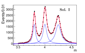
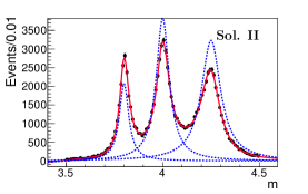
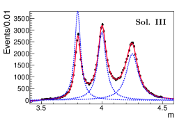
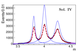
Figure 1: The four solutions from the fit to the toy MC produced mass spectra with the three interfering resonances included. The solid curves show the best fit and the dashed curves show the contributions from the three nonrelativistic BW components.

Table 1: Comparison between the extracted solution using mathematical method and that obtained from the fit with three interfering simple BW functions. A data sample of 100,000 events generated by toy MC is used in the fit.

Item	Sol. I (Input)	Fit I	Sol. II	Fit II	Sol. III	Fit III	Sol. IV	Fit IV
$\phi_{f}$	$\pi/3$	1.06	2.29	2.29	3.56	3.55	4.79	4.80
$\phi_{h}$	$3\pi/4$	2.37	6.02	6.02	5.66	5.67	3.05	3.05
$d$	1	—	0.81	—	0.46	—	0.37	—
$R_{z_{\alpha}}$	1/2	0.50	-0.89	-0.89	-0.81	-0.81	0.10	0.10
$I_{z_{\alpha}}$	$\sqrt{3}/2$	0.87	1.02	1.02	-0.36	-0.35	-1.19	-1.17
$R_{z_{\beta}}$	-$\sqrt{2}/2$	-0.72	1.20	1.19	0.60	0.60	-0.91	-0.91
$I_{z_{\beta}}$	$\sqrt{2}/2$	0.69	-0.32	-0.32	-0.43	-0.42	0.09	0.09
$M_{g}$	3.80	3.80	3.80	3.80	3.80	3.80	3.80	3.80
$\Gamma_{g}$	0.03	0.03	0.03	0.03	0.03	0.03	0.03	0.03
$M_{f}$	4.00	4.00	4.00	4.00	4.00	4.00	4.00	4.00
$\Gamma_{f}$	0.04	0.04	0.04	0.04	0.04	0.04	0.04	0.04
$M_{h}$	4.25	4.25	4.25	4.25	4.25	4.25	4.25	4.25
$\Gamma_{h}$	0.06	0.06	0.06	0.06	0.06	0.06	0.06	0.06

It is obvious that, for the case of three nonrelativistic BW amplitudes with interference, if one solution is known from the fit, the other three can be derived readily and numerically by solving Eq. (II).

IV.2 Relativistic BW amplitudes

For the case of relativistic BW amplitudes with interference, the values of the parameters as one solution are set as

$$M_{g}=4.20,\;\;\Gamma_{g}=0.09,$$

$$M_{f}=4.40,\;\;\Gamma_{f}=0.12,\;\;\phi_{f}=\pi/2,$$

$$M_{h}=4.60,\;\;\Gamma_{h}=0.18,\;\;\phi_{h}=3\pi/4.$$

The module of the amplitude squared of three interfering resonances is $\left|BW_{g}(m)+BW_{f}(m)e^{i\phi_{f}}+BW_{h}(m)e^{i\phi_{h}}\right|^{2}$ and the BW amplitudes use the formats shown in Eq. (15), where for the phase space factor we assume the reaction process is $e^{+}e^{-}\to\pi^{+}\pi^{-}J/\psi$. That is to say $z_{\alpha}=\sqrt{B_{f}\Gamma_{e^{+}e^{-}}^{f}/B_{g}\Gamma_{e^{+}e^{-}}^{g}}e^{i\phi_{f}}=i$ and $z_{\beta}=\sqrt{B_{h}\Gamma_{e^{+}e^{-}}^{h}/B_{g}\Gamma_{e^{+}e^{-}}^{g}}e^{i\phi_{h}}=-1/\sqrt{2}+1/\sqrt{2}i$ for the above solution, where the values of $B_{R}\Gamma^{R}_{e^{+}e^{-}}$ are set as 1 for $R=g,~{}f,$ and $h$.

According to the above probability density function and the first set of input solution, a data sample of 100,000 events is generated by using toy MC. Similarly, using the method mentioned earlier, another three sets of solutions can be found numerically, which are exactly repeated by fitting with the maximum likelihood method. The comparison of the results is shown in Table 2 and the fitted plots are shown in Fig. 2.

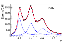
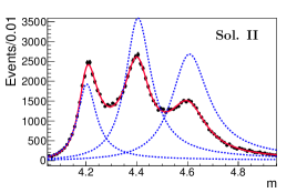
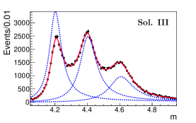
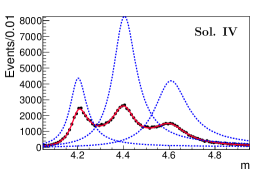
Figure 2: The four solutions from the fit to the toy MC produced mass spectra with the three interfering resonances included. The solid curves show the best fit and the dashed curves show the contributions from the three relativistic BW components.

Table 2: Comparison between the extracted solution using mathematical method and that from the fit with three interfering relativistic BW functions. A data sample of 100,000 events generated by toy MC is used in the fit.

Item	Sol. I (Input)	Fit I	Sol. II	Fit II	Sol. III	Fit III	Sol. IV	Fit IV
$\phi_{f}$	$\pi/2$	1.57	2.63	2.63	3.44	3.44	4.50	4.50
$\phi_{h}$	$3\pi/4$	2.36	6.14	6.14	5.12	5.12	2.62	2.62
$d$	1.00	—	0.77	—	0.45	—	0.35	—
$R_{z_{\alpha}}$	0.00	0.00	-1.43	-1.43	-0.98	-0.98	-0.35	-0.35
$I_{z_{\alpha}}$	1.00	1.00	0.80	0.80	-0.30	-0.30	-1.63	-1.63
$R_{z_{\beta}}$	-$1/\sqrt{2}$	-0.71	1.76	1.76	0.33	0.33	-1.31	-1.31
$I_{z_{\beta}}$	$1/\sqrt{2}$	0.71	-0.25	-0.25	-0.78	-0.78	0.75	0.75
$M_{g}$	4.20	4.20	4.20	4.20	4.20	4.20	4.20	4.20
$\Gamma_{g}$	0.09	0.09	0.09	0.09	0.09	0.09	0.09	0.09
$B_{g}\Gamma_{e^{+}e^{-}}^{g}$	1.00	1.03	1.29	1.30	2.20	2.21	2.85	2.85
$M_{f}$	4.40	4.40	4.40	4.40	4.40	4.40	4.40	4.40
$\Gamma_{f}$	0.12	0.12	0.12	0.12	0.12	0.12	0.12	0.12
$B_{f}\Gamma_{e^{+}e^{-}}^{f}$	1.00	1.02	3.46	3.45	2.29	2.28	7.94	7.94
$M_{h}$	4.60	4.60	4.60	4.60	4.60	4.60	4.60	4.60
$\Gamma_{h}$	0.18	0.18	0.18	0.18	0.18	0.18	0.18	0.18
$B_{h}\Gamma_{e^{+}e^{-}}^{h}$	1.00	1.01	4.07	4.07	1.60	1.60	6.53	6.52

V Discussion

As we found, when we need to describe a measured distribution using three interfering resonances $|g(x)+z_{\alpha}f(x)+z_{\beta}h(x)|^{2}/d$ , $F(x)=f(x)/g(x)$ and $H(x)=h(x)/g(x)$ satisfy the relation of Eq. (7). If $f(x)$, $h(x)$, and $g(x)$ are widely used BW functions, it has also been proved that such relation is exactly satisfied. In the case of three interfering resonances there occurred already four equivalent solutions with the same likelihood function minimum. Although the explicit analytical formulae can not be derived between different solutions, Eq. (II) can be utilized to derive the other three solutions numerically from the solution obtained by fitting. If three resonant amplitudes take simple or relativistic BW functions, two data samples generated by toy MC are used to cross check and verify our results. For other complicated BW functions, the relations Eqs. (7), (11), (II), and (II) still hold for $F(x)$ and $H(x)$. And for other forms of BW functions, with the coefficients obtained by Eqs. (7) and (11), the other solutions can be derived numerically by using the method mentioned earlier. The obtained numerical solutions agree well with those from the fit, which justifies our method. We believe with the help of finding other solutions numerically, it is easy to find all the solutions in real fits to the experimental distribution as long as the initial values of resonant parameters are set correctly.

References

• (1) X. L. Wang et al. (Belle Collaboration), Phys. Rev. D 91, 112007 (2015).
• (2) C. Z. Yuan, X. H. Mo and P. Wang, Int. J. Mod. Phys.  A 25, 5963 (2010).
• (3) K. Zhu, X. H. Mo, C. Z. Yuan, and P. Wang, Int. J. Mod. Phys. A. 26 4511 (2011).
• (4) A. D. Bukin, arXiv:0710.5627.
• (5) We provide an example on how to use mathematica software to solve Eq. (II) in order to derive the other three solutions from the already obtained one. The example can be downloaded in: http://shi.buaa.edu.cn/shencp/zh_CN/lwcg/7881/content/4850.htm
• (6) C. Patrignani et al. (Particle Data Group), Chin. Phys. C 40, 100001 (2016) and 2017 update.