Quantum anomaly and thermodynamics of one-dimensional
fermions with three-body interactions

Abstract

We show that a system of three species of one-dimensional fermions, with an attractive three-body contact interaction, features a scale anomaly directly related to the anomaly of two-dimensional fermions with two-body forces. We show, furthermore, that those two cases (and their multi-species generalizations) are the only non-relativistic systems with contact interactions that display a scale anomaly. While the two-dimensional case is well-known and has been under study both experimentally and theoretically for years, the one-dimensional case presented here has remained unexplored. For the latter, we calculate the impact of the anomaly on the equation of state, which appears through the generalization of Tan’s contact for three-body forces, and determine the pressure at finite temperature. In addition, we show that the third-order virial coefficient is proportional to the second-order coefficient of the two-dimensional two-body case.

Introduction.- The study of manifestations of scaling SO(2,1) anomalies in nonrelativistic systems has received considerable attention in recent years. Such anomalies appear when a symmetry is present at the classical level, but is broken by quantum fluctuations; the prime example in nonrelativistic physics is the two-dimensional (2D) Fermi gas with attractive contact interactions jackiw1991mab ; PitaevskiRosch ; Hofmann . On the experimental side, ultracold-atom experiments have shed light on the thermodynamic, collective-mode, and transport properties of that 2D system Experiments2D2010Observation ; Experiments2D2011Observation ; Experiments2D2011RfSpectroscopy ; Experiments2D2011DensityDistributionTrapped ; Experiments2D2011Crossover2D3D ; Experiments2D2012RfSpectraMolecules ; Experiments2D2012Crossover2D3D ; Experiments2D2012Polarons ; Experiments2D2012Viscosity ; ContactExperiment2D2012 ; Vale2Dcriteria ; Experiments2D2014 ; Experiments2D2015SpinImbalancedGas ; Experiments2D2015PairCondensation ; Experiments2D2015BKTObservation (see also RanderiaPairingFlatLand ; PieriDanceInDisk ). On the theory side, there have been multiple non-perturbative studies of basic ground-state  Bertaina ; ShiChiesaZhang ; Gezerlis and thermodynamic LiuHuDrummond ; Enss2D ; ParishEtAl ; AndersonDrut ; BarthHofmann quantities, and transport ChafinSchaefer ; EnssUrban ; EnssShear . In particular, Ref. UHetUNC2D spelled out the relationship between these anomalies and the Tan contact for 2D fermion systems with two-body contact interactions, and put forward a computational framework to access the shift of the virial coefficients $\Delta b_{n}$, $n\geq 2$ using a Hubbard-Stratonovich transformation.

In this work, we show that a system of one-dimensional (1D) fermions with an attractive three-body contact interaction presents a scaling anomaly of the same kind as that of the 2D case with two-body forces. Naturally, the system is non-trivial only if at least three fermion species are present in the problem, which implies straightforward results (e.g., the virial coefficients are non-trivial starting at third order) as well as more challenging aspects (namely dealing with a three-body problem for any useful calculation). While here we consider unpolarized distinguishable species (no mass asymmetry or population imbalance), generalizations to more species and asymmetric cases could and should also be studied.

Hamiltonian.- The system is defined by the following Hamiltonian

$$\hat{H}=\!\!\!\!\sum_{s=1,2,3}\int dp\;\epsilon(p)\;\hat{a}_{s,p}^{\dagger}\hat{a}_{s,p}+g\int dx\;\hat{n}_{1}(x)\hat{n}_{2}(x)\hat{n}_{3}(x),$$ (1)

where $\epsilon(p)=\frac{\hbar^{2}p^{2}}{2m}$. Here, $\hat{a}_{s,p}^{\dagger}$ and $\hat{a}_{s,p}$ are the creation and annihilation operators for particles of species $s$ and momentum $p$, and $\hat{n}_{s}(x)$ is the corresponding density at position $x$. In what follows we will take $\hbar=k_{B}=m=1$ (we will, however, show $m$ in the following equations in order to distinguish it from the total and reduced masses). A crucial feature of this system is that, since the 1D density has units of inverse length, the bare coupling $g$ is dimensionless. As we show below, however, the coupling runs non-trivially with the cutoff, and the physical coupling (dimensionally transmuted scale Camblong ) is the binding energy of the three-body system.

Renormalization and the three-body problem.- As anticipated, in order to renormalize the problem we determine the connection between the bare coupling $g$ and the binding energy $\epsilon_{B}$ of the three-body system. We will show here that the system forms such a three-body bound state at arbitrarily small $g$, and we will do so by mapping our problem onto a 2D one-body problem interacting with an external Dirac delta potential. That problem is of course what results from considering a two-body problem with a two-body delta function interaction, when going to the center-of-mass frame.

The 1D three-particle Schrödinger equation for our system takes the form

$$\left[-\frac{\nabla^{2}_{X}}{2m}+g\delta(x_{2}-x_{1})\delta(x_{3}-x_{2})\right]\psi(X)=E\psi(X)$$ (2)

where we used the shorthand notation $X=(x_{1},x_{2},x_{3})$ and $\nabla^{2}_{X}=\frac{\partial^{2}}{\partial x_{1}^{2}}\!+\!\frac{\partial^{2}}{\partial x_{2}^{2}}\!+\!\frac{\partial^{2}}{\partial x_{3}^{2}}$. One way to see the equivalence advertised above is already evident at this point: Eq. (2) corresponds to a 3D one-body problem (if we identify the coordinates by $(x,y,z)=(x_{1},x_{2},x_{3})$) with an external line-like delta potential saturating at $x=y=z$. By symmetry, we may factorize such a 3D problem into a trivial part for the unrestricted motion parallel to the line, and a non-trivial part for the 2D motion perpendicular to the line (which sees a point-like delta potential). As we show below, that factorization corresponds in the 1D problem to the center-of-mass (CM) and relative motions.

To be explicit, we proceed by separating the CM motion by the change of variables $Q=\frac{1}{3}(x_{1}+x_{2}+x_{3})$; $q_{1}=x_{2}-x_{1}$; $q_{2}=\frac{1}{{\sqrt{3}}}(x_{1}+x_{2}-2x_{3})$. Writing $\psi(X)=\Phi(Q)\phi(q_{1},q_{2})$, we obtain an equation for the CM motion, as usual,

$$\frac{-\nabla^{2}_{Q}}{2{M}}\Phi(Q)=E_{\text{CM}}\Phi(Q),$$ (3)

where $M=3m$. For the relative coordinates $q_{1}$, $q_{2}$ [Note $q_{2}=(2/\sqrt{3})(x_{2}-x_{3})$ when $q_{1}=x_{2}-x_{1}=0$],

$$\left[\frac{-\nabla^{2}_{q}}{2\bar{m}}+\tilde{g}\delta(q_{1})\delta(q_{2})\right]\phi(q_{1},q_{2})=E_{r}\phi(q_{1},q_{2}),$$ (4)

where $\bar{m}=m/2$ is the reduced mass, $\tilde{g}=(2/\sqrt{3})g$, is the effective coupling, $E_{r}$ is the energy of relative motion, and $\nabla^{2}_{q}=\frac{\partial^{2}}{\partial q_{1}^{2}}+\frac{\partial^{2}}{\partial q_{2}^{2}}$, which thus reduces the problem to that of a single particle in 2D with a delta function potential at the origin. The problem is easily solved in momentum space, where one finds that the wavefunction takes the form $\tilde{\phi}({\bf p})\propto 1/({\bf p}^{2}-E_{r})$, and the binding energy $\epsilon_{B}=-E_{r}$ of the three-body bound state (trimer) depends on the coupling as

$$\frac{\epsilon_{B}}{\Lambda^{2}}=e^{4\pi/\tilde{g}},$$ (5)

where $\tilde{g}<0$, and $\Lambda$ is a momentum cutoff that is required to regularize ultraviolet divergences. Using the above relation, one identifies the trimer binding energy $\epsilon_{B}$ as the physical coupling, and as the emerging scale that breaks scale invariance.

It is noteworthy that for $n$-body contact interactions in $d$ dimensions, the units of the bare coupling are $L^{-2+d(n-1)}$, such that there are only two physically relevant solutions for which the coupling is dimensionless: $n=d=2$, i.e. the 2D case with a two-body interaction, and $n=3$, $d=1$, which is the 1D case shown here.

Below, we will use a lattice regularization of the problem to arrive at many-body results. In that case, the relation between the bare lattice coupling $g_{\text{lat}}$ and the binding energy is given implicitly by

$$\frac{1}{g_{\text{lat}}}=-\frac{1}{L^{2}}\sum_{\bf k}\frac{1}{\epsilon_{\bf k}+\epsilon_{B}},$$ (6)

where $L=N_{x}\ell$ is the lattice size, $\ell$ is the lattice spacing, $\epsilon_{\bf k}=(k_{1}^{2}+k_{2}^{2}+k_{3}^{2})/2$, ${\bf k}=(2\pi/L)(n_{1},n_{2},n_{3})$, and the sum covers $0\leq|n_{1}+n_{2}|\leq\Lambda$, with the constraint $n_{1}+n_{2}+n_{3}=0$ (i.e. vanishing total momentum).

Results.- Anomaly in the equation of state. In truly scale invariant systems, such as noninteracting ones, the pressure $P$ may be written in terms of the inverse temperature $\beta$ and the chemical potential $\mu$ as $P=\beta^{\alpha}f(\beta\mu)$, where $\alpha=-d/2-1$ and $d$ is the number of spatial dimensions. The advantage of isolating the dependence on the dimensionful parameter $\beta$ is that one readily derives, using thermodynamic identities and partial differentiation with respect to $\beta$ and $\mu$, the well-known result

$$P=\frac{2}{d}\frac{E}{V},$$ (7)

where $E$ is the total energy and $V$ is the $d$-dimensional volume. In scale-anomalous systems like the one put forward here, the pressure acquires a second physical, dimensionless parameter via the anomaly, which we will write as $\beta\epsilon_{B}$, where $\epsilon_{B}$ is the binding energy of the three-body problem described above. Thus, $P=\beta^{\alpha}f(\beta\mu,\beta\epsilon_{B})$. Following the same derivation outlined above, one can easily see that

$$P-\frac{2}{d}\frac{E}{V}=\frac{2}{d}\beta^{\alpha}\frac{\partial f}{\partial(\beta\epsilon_{B})}\beta\epsilon_{B}=\frac{2}{d}\beta^{\alpha}\frac{\partial f}{\partial\ln(\beta\epsilon_{B})},$$ (8)

which shows that the emergence of the second parameter results in a contribution to the equation of state that breaks the scale invariant result of Eq. (7).

Anomaly as Tan’s contact. Specializing to our case, the anomalous term in Eq. (8) is proportional to a generalization of Tan’s contact to the case of 3-body forces. Indeed, since $\beta PV=\ln\mathcal{Z}$, where $V=L$ is the volume and $\mathcal{Z}=\text{Tr}\exp\left[-\beta(\hat{H}-\mu\hat{N})\right]$ is the grand-canonical partition function, the only way in which $f$ can depend on $\epsilon_{B}$ is through the dimensionless bare coupling $g$ that appears in $\hat{H}$:

$$\frac{\partial f}{\partial\ln(\beta\epsilon_{B})}=\frac{\sqrt{\beta}}{L}\frac{\partial\ln\mathcal{Z}}{\partial g}\frac{\partial g}{\partial\ln(\beta\epsilon_{B})},$$ (9)

where

$$\frac{1}{\beta L}\frac{\partial\ln\mathcal{Z}}{\partial g}=-\langle\hat{n}_{1}\hat{n}_{2}\hat{n}_{3}\rangle,$$ (10)

and the angle brackets denote a thermal expectation value in the grand-canonical ensemble. Thus, for our scale-anomalous 1D system

$$P-2\frac{E}{L}={\mathcal{C}_{3}},$$ (11)

where we have identified

$$\mathcal{C}_{3}=2\frac{\partial P}{\partial\ln(\beta\epsilon_{B})}=-2\frac{\partial g}{\partial\ln(\beta\epsilon_{B})}\langle\hat{n}_{1}\hat{n}_{2}\hat{n}_{3}\rangle,$$ (12)

as the generalization of Tan’s contact density for the case of three-body forces TanContact ; Valiente ; ContactReview ; WernerCastin . Note that the dimensions of the contact density are those of pressure or energy density, which in 1D amounts to $1/L^{3}$. Thus, the contact factorizes into a three-body piece (the change in the bare coupling with the physical coupling) and a many-body piece (the expectation value of the triple density operator). Note that, in the continuum, from Eq. (5) we find

$$\frac{\partial g}{\partial\ln(\beta\epsilon_{B})}=-\frac{1}{2\pi\sqrt{3}}g^{2}.$$ (13)

On the lattice, using the relationship between $g_{\text{lat}}$ and $\epsilon_{B}$,

$$\frac{\partial g_{\text{lat}}}{\partial\ln(\beta\epsilon_{B})}=-g^{2}_{\text{lat}}\frac{1}{L^{2}}\sum_{\bf k}\frac{\epsilon_{B}}{(\epsilon_{\bf k}+\epsilon_{B})^{2}}.$$ (14)

where the sum is constrained in the same way as that of Eq. (6).

Virial coefficients and high-temperature thermodynamics. Because the system proposed here contains no two-body forces, the coefficients $b_{n}$ of the virial expansion are identical to those of the non-interacting case up to second order: $b_{1}=1$; $b_{2}=b_{2}^{(0)}$, where in general $b_{n}^{(0)}=(-1)^{n+1}/n^{3/2}$. The third-order coefficient $b_{3}$ and above, however, are directly affected by the anomaly. Indeed, if the interacting $n$-body partition function is $Q_{n}$, the first nontrivial one in our system is $Q_{3}$. Therefore,

$$\Delta b_{3}\equiv b_{3}-b_{3}^{(0)}=\frac{\Delta Q_{3}}{Q_{1}},$$ (15)

where $b_{3}^{(0)}$ is the noninteracting third order virial coefficient, and we have used the definition $b_{3}\equiv{Q_{3}}/{Q_{1}}-Q_{2}+Q_{1}^{2}/3$ together with the fact that $Q_{1}$ and $Q_{2}$ are unaffected by the three-body interaction. Moreover, $\Delta Q_{3}=\Delta Q_{1,1,1}$, where $Q_{n_{1},n_{2},n_{3}}$ is the partition function of the system with $n_{j}$ particles of species $j$. In translation-invariant systems it is always possible to factor out the center-of-mass motion, such that $\Delta Q_{3}=Q_{3}^{\text{CM}}\Delta Q_{1,1,1}^{\text{rel}}$, where $Q_{3}^{\text{CM}}=\sqrt{3}L/\lambda_{T}$ and $\lambda_{T}=\sqrt{2\pi\beta}$. Similarly, the two-body 2D case satisfies

$$\Delta b_{2}^{\text{2D}}\equiv b^{\text{2D}}_{2}-b_{2}^{(0),\text{2D}}=\frac{\Delta Q^{\text{2D}}_{2}}{Q^{\text{2D}}_{1}}=\frac{Q_{2}^{\text{CM,2D}}\Delta Q^{\text{rel, 2D}}_{1,1}}{Q^{\text{2D}}_{1}},$$ (16)

where $Q_{2}^{\text{CM,2D}}=2L^{2}/\lambda_{T}^{2}$. Since we showed above that the relative motion of the three-body 1D problem is captured by the dynamics of the two-body problem in 2D, we have (at fixed $\beta\epsilon_{B}$), $\Delta Q_{1,1,1}^{\text{rel}}=\Delta Q_{1,1}^{\text{rel,2D}}$. Thus, putting together the above equations we arrive at

$$\Delta b_{3}=\frac{Q_{3}^{\text{CM}}}{Q_{1}}\frac{Q^{\text{2D}}_{1}}{Q_{2}^{\text{CM,2D}}}\Delta b_{2}^{\text{2D}}=\frac{\Delta b_{2}^{\text{2D}}}{\sqrt{3}},$$ (17)

where we used the expressions for the 1D, three-flavor single-particle partition function $Q_{1}=3L/\lambda_{T}$, and the 2D, two-flavor analogue $Q^{\text{2D}}_{1}=2L^{2}/\lambda^{2}_{T}$. It is important to note that the factor of $1/\sqrt{3}$ in the above equation relating $\Delta b_{3}$ and $\Delta b_{2}^{\text{2D}}$ is unrelated to the factor of $2/\sqrt{3}$ that appears in the relationship between $g$ and $\tilde{g}$.

From the above considerations we obtain the high-temperature (strictly speaking low-fugacity) behavior of the pressure and Tan’s contact using the corresponding virial expansions, namely

$$\beta L(P-P_{0}) = Q_{1}\sum_{k=1}^{\infty}\Delta b_{k}z^{k}$$ (18)

$$\beta L{\mathcal{C}_{3}} = Q_{1}\sum_{k=1}^{\infty}c_{k}z^{k},$$ (19)

where $c_{k}=2\partial b_{k}/\partial\ln(\beta\epsilon_{B})$.

In addition, the relationship between $\Delta b_{2}^{\text{2D}}$ and $\Delta b_{3}$ yields the thermodynamics of the three-body problem, since the change in the corresponding partition function is

$$Q_{3}-Q_{3}^{(0)}=Q_{1}\Delta b_{3},$$ (20)

where $Q_{3}^{(0)}=(Q_{1}/3)^{3}$.

Toward the many-body properties. Despite the close connection between the 1D and 2D problems explained above, in particular at the few-body level, the many-body properties certainly differ (e.g. we expect a superfluid transition in the 2D case, while no such behavior would appear in our 1D system). To provide a first look at the thermodynamics, we present here perturbative results for the pressure at finite temperature and density.

To obtain those results, we put the system on a spacetime lattice and use a Hubbard-Stratonovich transformation to represent the interaction. Specifically, we write for a given point in spacetime,

$$e^{-\tau g_{\text{lat}}\hat{n}_{1}\hat{n}_{2}\hat{n}_{3}}=\int_{\Gamma}\frac{d\sigma}{3\pi}\prod_{j=1,2,3}(1+B\hat{n}_{j}f(\sigma)),$$ (21)

where $\Gamma=[{-3\pi/2},{3\pi/2}]$, $f(\sigma)=e^{i2\sigma/3}\cos^{2}\sigma$, $B^{3}=C(e^{-\tau g_{\text{lat}}}-1)$ with $C=64/15$, $g_{\text{lat}}$ is the lattice bare coupling, and $\tau$ is the temporal lattice spacing. Using this transformation, we may write the partition function as

$$\mathcal{Z}=\int\mathcal{D}\sigma\;{\det}^{3}M[\sigma],$$ (22)

where the matrix $M[\sigma]$ is the usual fermion matrix encoding the dynamics and input parameters, including the fugacity $z$. One may use this formulation of the many-body problem to carry out Monte Carlo calculations Drut:2012md ; QMCReviews ; however, the imaginary parts of $f(\sigma)$ imply that there would be a so-called phase problem. Instead, for such calculations one should resort to fixed-node methods, which we will carry out elsewhere. Here, we evaluate the pressure at next-to-leading order in perturbation theory, as we outline next. Expanding the effective action $S[\sigma]=-3\ln\det M[\sigma]$ in powers of $B$, along the lines of the work of Ref. PRDAndrew , and keeping only the leading contribution, we obtain

$$\ln(\mathcal{Z}/\mathcal{Z}_{0})=N_{\tau}N_{x}\ln\left[\int_{\Gamma}\frac{d\sigma}{3\pi}\exp(3KBf(\sigma))\right],$$ (23)

where

$$K=\frac{1}{N_{x}}\sum_{p}\frac{ze^{-\beta p^{2}/2}}{1+ze^{-\beta p^{2}/2}},$$ (24)

all of which is evaluated numerically. To renormalize the coupling, we compute the change in the third-order virial coefficient in our approximation and tune $g_{\text{lat}}$ to match the exact $\Delta b_{3}$ derived above, and thus obtain the physical coupling $\beta\epsilon_{B}$. Using $\ln(\mathcal{Z}/\mathcal{Z}_{0})=\beta V(P-P_{0})$, in Fig. 1 we show $P/P_{0}$ as a function of $\beta\mu$ for $\beta\epsilon_{B}=0.1$, alongside the virial expansion, to illustrate the shape of the equation of state of this system. The increase $P/P_{0}$ as a function of $\beta\mu$ is characteristic of systems with attractive interactions (see e.g. EoS1D ; AndersonDrut ).

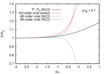
Figure 1: Solid line: Pressure, in units of of the noninteracting counterpart, of the 1D anomalous many-body system at $\beta\epsilon_{B}=0.1$, as a function of $\beta\mu$. The various virial-expansion results show the exact contribution up to third order ($\Delta b_{3}$ was used to tune the lattice coupling), and perturbative results up to fourth and fifth orders from the evaluation of the pressure at next-to-leading order in lattice perturbation theory.

Due to the formation of three-body bound states at vanishingly small attractive coupling, we expect to have an effective description in terms of composite fermions, i.e. trimers at strong coupling. As the trimer states become localized with increased coupling, Pauli exclusion dictates that their interaction should be repulsive. Thus, we expect a behavior that is rather different from the fermion-boson crossover phenomenon featured in 2D; instead, we expect a fermion–trimer crossover, where both ends are of fermionic character. For weak attraction, where the trimers are loosely bound, the trimer-trimer interaction may be attractive, which would result in trimer pairing. At fixed $\ln(\epsilon_{B}/\epsilon_{F})$, there should exist a crossover temperature $T^{*}$ above which the trimers break into unbound fermions.

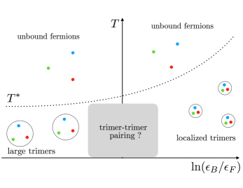
Figure 2: Conjectured many-body behavior of the 1D anomalous system as a function of temperature $T$ and dimensionless coupling $\ln(\epsilon_{B}/\epsilon_{F})$, where $\epsilon_{F}$ is the Fermi energy. At low temperatures, the system forms large trimers (at weak coupling) and localized repulsive trimers (point-like identical fermions, at strong coupling). Whether the attractive interaction is enough to overcome Pauli exclusion and lead to trimer-trimer pairing, it remains an open question. At high enough temperatures (crossover pictured here as $T^{*}$), the effective description should be in terms of unbound fermions with residual three-body correlations.

Finally, the more general situation where the particle population is asymmetric, e.g. majority or minority type 1 and equal population of types 2 and 3, or all different, may lead to a variety of situations (e.g. fermion-mediated attractive interaction between dimers), to be explored elsewhere.

Summary and Conclusions.- We have shown that a system of 1D fermions with an attractive three-body contact interaction features a scale invariance which, while present at the classical level (the coupling $g$ is dimensionless), is broken by quantum fluctuations which generate a three-body bound state at arbitrarily small couplings. To show it, we mapped the three-body 1D problem to a two-body 2D problem (or, rather, both are mapped onto the same one-body 2D problem in a Dirac delta potential). Thus, this system presents a scale anomaly in a remarkable way: it lives in 1D but it is locally (around any region where particles scatter) like its 2D two-body counterpart, which is reminiscent of the concept of holography. We have shown that the anomaly is directly related to Tan’s contact, which introduces a change in the equation of state in a way that is essentially identical to that of the 2D case. In addition, we have shown that the third order virial coefficient of our 1D system is proportional to the second-order coefficient of the 2D system. Finally, we provide an initial look into the many-body properties with a perturbative calculation of the pressure, and conjecture an overall picture of the physics of the system in the temperature-coupling plane.

We acknowledge useful discussions with L. Dolan, A. C. Loheac, and C. R. Shill. This work was supported by the U.S. National Science Foundation under Grant No. PHY1452635 (Computational Physics Program). This work was supported in part by the US Army Research Office Grant No. W911NF-15-1-0445.

References

- (1) R. Jackiw, in MAB Beg Memorial Volume , edited by A. Ali and P. Hoodbhoy (1991) p. 35.
- (2) L.P. Pitaevskii, A. Rosch, Phys. Rev. A 55, R 835 (1997).
- (3) J. Hofmann, Phys. Rev. Lett. 108, 185303 (2012); E. Taylor and M. Randeria, Phys. Rev. Lett. 109, 135301 (2012); Phys. Rev. Lett. 110, 089904 (2013);
- (4) K. Martiyanov, V. Makhalov, and A. Turlapov, Phys. Rev. Lett. 105, 030404 (2010).
- (5) M. Feld, B. Fröhlich, E. Vogt, M. Koschorreck, and M. Köhl, Nature (London) 480, 75 (2011).
- (6) B. Fröhlich, M. Feld, E. Vogt, M. Koschorreck, W. Zwerger, and M. Köhl, Phys. Rev. Lett. 106, 105301 (2011).
- (7) S.K. Baur, B. Fröhlich, M. Feld, E. Vogt, D. Pertot, M. Koschorreck, and M. Köhl, Phys. Rev. A 85, 061604 (2012).
- (8) P. Dyke, E.D. Kuhnle, S. Whitlock, H. Hu, M. Mark, S. Hoinka, M. Lingham, P. Hannaford, and C. J. Vale, Phys. Rev. Lett. 106, 105304 (2011).
- (9) A. T. Sommer, L. W. Cheuk, M. J. H. Ku, W. S. Bakr, and M. W. Zwierlein, Phys. Rev. Lett. 108, 045302 (2012).
- (10) Y. Zhang, W. Ong, I. Arakelyan, and J. E. Thomas, Phys. Rev. Lett. 108, 235302 (2012); M. Koschorreck, D. Pertot, E. Vogt, B. Fröhlich, M. Feld, and M. Köhl, Nature (London) 485, 619 (2012);
- (11) A. A. Orel, P. Dyke, M. Delehaye, C. J. Vale, and H. Hu, New J. Phys. 13, 113032 (2011).
- (12) E. Vogt, M. Feld, B. Fröhlich, D. Pertot, M. Koschorreck, M. Köhl, Phys. Rev. Lett. 108, 070404 (2012).
- (13) B. Fröhlich, M. Feld, E. Vogt, M. Koschorreck, M. Köhl, C. Berthod, and T. Giamarchi, Phys. Rev. Lett. 109, 130403 (2012).
- (14) P. Dyke, K. Fenech, T. Peppler, M. G. Lingham, S. Hoinka, W. Zhang, B. Mulkerin, H. Hu, X.-J. Liu, C. J. Vale, arXiv:1411.4703.
- (15) V. Makhalov, K. Martiyanov, A. Turlapov, Phys. Rev. Lett. 112, 045301 (2014).
- (16) W. Ong, C. Cheng, I. Arakelyan, and J. E. Thomas, Phys. Rev. Lett. 114, 110403 (2015).
- (17) M. G. Ries, A. N. Wenz, G. Zürn, L. Bayha, I. Boettcher, D. Kedar, P. A. Murthy, M. Neidig, T. Lompe, and S. Jochim, Phys. Rev. Lett. 114, 230401 (2015).
- (18) P .A. Murthy, I. Boettcher, L. Bayha, M. Holzmann, D. Kedar, M. Neidig, M. G. Ries, A. N. Wenz, G. Zürn, S. Jochim, Phys. Rev. Lett. 115, 010401 (2015).
- (19) M. Randeria, Physics 5, 10 (2012).
- (20) P. Pieri, Physics 8, 53 (2015).
- (21) G. Bertaina and S. Giorgini, Phys. Rev. Lett. 106, 110403 (2011).
- (22) H. Shi, S. Chiesa, and S. Zhang, Phys. Rev. A 92, 033603 (2015).
- (23) A. Galea, H. Dawkins, S. Gandolfi, A. Gezerlis, Phys. Rev. A 93, 023602 (2016).
- (24) X.-J. Liu, H. Hu, and P. D. Drummond, Phys. Rev. B 82, 054524 (2010).
- (25) M. Bauer, M. M. Parish, and T. Enss, Phys. Rev. Lett. 112, 135302 (2014).
- (26) V. Ngampruetikorn, J. Levinsen, and M. M. Parish, Phys. Rev. Lett. 111, 265301 (2013).
- (27) E. R. Anderson, J. E. Drut, Phys. Rev. Lett. 115, 115301 (2015)
- (28) M. Barth and J. Hofmann, Phys. Rev. A 89, 013614 (2014).
- (29) C. Chafin and T. Schäfer Phys. Rev. A 88, 043636 (2013).
- (30) S. Chiacchiera, D. Davesne, T. Enss, and M. Urban, Phys. Rev. A 88, 053616 (2013).
- (31) T. Enss, C. Küppersbusch, L. Fritz, Phys. Rev. A 86, 013617 (2012).
- (32) W. S. Daza, J. E. Drut, C. L. Lin, C. R. Ordóñez, arXiv:1801.08086
- (33) H. E. Camblong, L. N. Epele, H. Fanchiotti, C. A. Garcia Canal Ann. Phys. 287, 14 (2001).
- (34) S. Tan, Ann. Phys. 323, 2952 (2008); ibid. 323, 2971 (2008); ibid. 323, 2987 (2008); S. Zhang, A. J. Leggett, Phys. Rev. A 77, 033614 (2008); F. Werner, Phys. Rev. A 78, 025601 (2008); C. Langmack, M. Barth, W. Zwerger, E. Braaten, Phys. Rev. Lett. 108, 060402 (2012).
- (35) M. Valiente, N. T. Zinner, and K. Mølmer, Phys. Rev. A 84, 063626 (2011); Phys. Rev. A 86, 043616 (2012).
- (36) F. Werner and Y. Castin, Phys. Rev. A 86, 013626 (2012). E. Braaten, in The BCS-BEC Crossover and the Unitary Fermi Gas, edited by W. Zwerger (Springer-Verlag, 2012). X.-J. Liu Phys. Rep. 524, 37 (2013).
- (37) F. Werner and Y. Castin, Phys. Rev. A 86, 013626 (2012).
- (38) J. E. Drut and A. N. Nicholson, J. Phys. G 40, 043101 (2013).
- (39) D. Lee, Phys. Rev. C 78, 024001 (2008); Prog. Part. Nucl. Phys. 63, 117 (2009).
- (40) A. C. Loheac and J. E. Drut, Phys. Rev. D 95, 094502 (2017).
- (41) M. D. Hoffman, P. D. Javernick, A. C. Loheac, W. J. Porter, E. R. Anderson, and J. E. Drut. Phys. Rev. A 91, 033618 (2015).