$C^{1,\alpha}$ regularity for fully nonlinear elliptic equations with superlinear growth in the gradient

Abstract. We extend the Caffarelli-Świech-Winter $C^{1,\alpha}$ regularity estimates to $L^{p}$-viscosity solutions of fully nonlinear uniformly elliptic equations in nondivergence form with superlinear growth in the gradient and unbounded coefficients. As an application, in addition to the usual $W^{2,p}$ results, we prove the existence of positive eigenvalues for proper operators with nonnegative unbounded weight, in particular for Pucci’s operators with unbounded coefficients.

Résumé. Dans cet article on étend les résultats de régularité $C^{1,\alpha}$ de Caffarelli-Świech-Winter aux solutions de $L^{p}$ viscosité des équations complètement non-linéaires, uniformément elliptiques, sous forme non-divergence, avec croissance super-linéaire par rapport au gradient et coefficients non bornés. Dans le cadre d’une application, en plus des résultats habituels $W^{2,p}$, on prouve l’existence de valeurs propres positives pour les opérateurs propres avec poids non borné non négatif, en particulier pour les opérateurs de Pucci à coefficients non bornés.

Keywords. Regularity, Estimates, Superlinear gradient growth, Nondivergence form.

MSC2010. 35J15, 35B65, 35J60, 35P30, 35P15.

1 Introduction

The seminal work of Caffarelli [13] in 1989 brought an innovative approach of looking at Schauder type results via iterations from the differential quotients that are perturbations of solutions of the respective autonomous equations. The techniques in [13], which contains in particular $C^{1,\alpha}$ estimates for $L^{p}$-viscosity solutions of uniformly elliptic equations $F(x,D^{2}u)=f(x)$, allowed Świech [50] to extend them to more general operators $F(x,u,Du,D^{2}u)$ and later Winter [56] to boundary and global bounds. However, everything that is available in the literature, to our knowledge, for $L^{p}$-viscosity solutions in the fully nonlinear framework, concerns only structures with either linear gradient growth or bounded coefficients, except for some particular cases of extremal equations with small coefficients, see [32]. It is our goal here to obtain $C^{1,\alpha}$ regularity and estimates for general fully nonlinear uniformly elliptic equations, with at most quadratic growth in the gradient and unbounded coefficients.

The study of such quasilinear elliptic equations with quadratic dependence in the gradient had its beginning in the ’80s, essentially with the works of Boccardo, Murat and Puel [9], [10] and became a relevant research topic which still develops. This type of nonlinearity often appears in risk-sensitive stochastic problems, as well as in large deviations, control and game theory, mean-fields problems. Moreover, the class of equations in the form $Lu=g(x,u,Du)$, where $L$ is a second order general operator and $g$ has quadratic growth in the gradient, is invariant under smooth changes of the function $u$ and the variable $x$. Due to this fact, this class is usually referred as having natural growth in the gradient.

Rather complete $C^{\alpha}$ regularity results for fully nonlinear uniformly elliptic equations with up to quadratic growth in the gradient were obtained in [47], in the most general setting of unbounded coefficients, for $L^{p}$-viscosity solutions. Then, the question of $C^{1,\alpha}$ regularity for the same class arises naturally. In the present work we show, as can be expected, that $C^{1,\alpha}$ regularity and estimates are valid in this context. These $C^{1,\alpha}$ estimates are instrumental in the recent study of multiplicity for nonproper equations in [40].

We note that Trudinger, independently from [13], in [53] proved $C^{1,\alpha}$ regularity in a less general scenario than Świech and Winter, under a continuity hypothesis for $F$, dealing with $C$-viscosity solutions and approximations under supconvolutions. In that paper, it was stated that a priori estimates for solutions in $C^{1,\alpha}$ of superlinear equations could be derived from the arguments in [53] and [52]. However, the question of regularity is more complicated (for a discussion on differences between a priori bounds and regularity results we refer to [45]).

We also quote some other papers on $C^{1,\alpha}$ regularity, the classical works [33], [35], [36] for linear equations, [38] for Neumann boundary conditions, [46] for asymptotically convex operators, [24] (local) and [8] (global) for degenerate elliptic operators, [16] and [34] for parabolic equations possibly with VMO coefficients. Furthermore, Wang [55] has made an important contribution to $C^{1,\alpha}$ regularity for the parabolic equation $u_{t}+F(x,D^{2}u)=g(t,x,Du)$, where $|g(t,x,p)|\leq A\,|p|^{2}+g(t,x)$, for bounded coefficients, see lemma 1.6 in [55] (which uses theorem 4.19 in [54]). Sharp regularity results for general parabolic equations with linear gradient growth can be found in [17], and very complete $C^{1,\alpha}$ estimates on the boundary for solutions in the so called $S^{*}$-class for equations with linear gradient growth and unbounded coefficients in [11].

It is also essential to mention an important series of papers due to Koike and Świech [29], [30], [31], [32], in which they proved ABP and weak Harnack inequalities for $L^{p}$-viscosity solutions of equations with superlinear growth in the gradient, together with several theorems about existence, uniqueness and $W^{2,p}$ estimates for solutions of extremal equations involving Pucci’s operators with unbounded coefficients, see in particular theorem 3.1 in [32]. Many of our arguments depend on the machinery in these works.

Next we list our hypotheses. For $F(x,r,p,X)$ measurable in $x$, we consider the general structure condition

$$\mathcal{M}_{\lambda,\Lambda}^{-}(X-Y)-b(x)|p-q|-\mu|p-q|(|p|+|q|)-d(x)\,\omega(|r-s|)$$

$$\leq F(x,r,p,X)-F(x,s,q,Y) (SC)^{\mu}$$

$$\leq\mathcal{M}_{\lambda,\Lambda}^{+}(X-Y)+b(x)|p-q|+\mu|p-q|(|p|+|q|)+d(x)\,\omega(|r-s|)\;\textrm{ for }x\in\Omega$$

where $F(\cdot,0,0,0)\equiv 0$ and $0<\lambda\leq\Lambda$, $b\in L^{p}_{+}(\Omega)$ for some $p>n$, $d\in L^{\infty}_{+}(\Omega)$, $\mu\geq 0$ and $\omega$ is a modulus of continuity (see section 2).

In order to measure the oscillation of $F$ in the $x$ entry, we define, as in [13], [56],

$$\beta(x,x_{0})=\beta_{F}(x,x_{0}):=\sup_{X\in\mathbf{S}^{n}\setminus\{0\}}\frac{|F(x,0,0,X)-F(x_{0},0,0,X)|}{\|X\|}.$$ (1.1)

Notice that $\beta$ is a bounded function by 1 and consider the usual hypothesis, as in [13], [56]: given $\theta>0$, there exists $r_{0}=r_{0}\,(\theta)>0$ such that

$$\;\left(\frac{1}{r^{n}}\int_{B_{r}(x_{0})\cap\Omega}\beta(x,x_{0})^{p}\;\mathrm{d}x\right)^{\frac{1}{p}}\leq\theta\,,\;\textrm{ for all }r\leq r_{0}. H_{\theta}$$ ()

The following is our main result. To simplify its statement, here we assume $\omega(r)\leq\omega(1)r$ for all $r\geq 0$.

Theorem 1.1.

Assume $F$ satisfies 1, $f\in L^{p}(\Omega)$, where $p>n$, and $\Omega\subset{\mathbb{R}^{n}}$ is a bounded domain. Let $u$ be an $L^{p}$-viscosity solution of

$$F(x,u,Du,D^{2}u)=f(x)\quad\textrm{ in }\;\Omega$$ (1.2)

with $\|u\|_{L^{\infty}(\Omega)}+\|f\|_{L^{p}(\Omega)}\leq C_{0}$. Then, there exists $\alpha\in(0,1)$ and $\theta=\theta(\alpha)$, depending on $n,p,\lambda,\Lambda,\|b\|_{L^{p}(\Omega)}$, such that if ($H_{\theta}$) holds for all $r\leq\min\{r_{0},\mathrm{dist}(x_{0},\partial\Omega)\}$, for some $r_{0}>0$ and for all $x_{0}\in\Omega$, this implies that $u\in C^{1,\alpha}_{\mathrm{loc}}(\Omega)$ and for any subdomain $\Omega^{\prime}\subset\subset\Omega$,

$$\|u\|_{C^{1,\alpha}(\overline{\Omega^{\prime}})}\leq C\,\{\|u\|_{L^{\infty}(\Omega)}+\|f\|_{L^{p}(\Omega)}\}$$ (1.3)

where $C$ depends only on $\,r_{0},n,p,\lambda,\Lambda,\alpha,\mu,\|b\|_{L^{p}(\Omega)},\omega(1)\|d\|_{L^{\infty}(\Omega)},\mathrm{diam}(\Omega)$, $\mathrm{dist}(\Omega^{\prime},\partial\Omega),C_{0}$.

If in addition, $\partial\Omega\in C^{1,1}$ and $u\in C(\overline{\Omega})\cap C^{1,\tau}(\partial\Omega)$ is such that and $\|u\|_{L^{\infty}(\Omega)}+\|f\|_{L^{p}(\Omega)}+\|u\|_{C^{1,\tau}(\partial\Omega)}\leq C_{1}$, then there exists $\alpha\in(0,\tau)$ and $\theta=\theta(\alpha)$, depending on $n,p,\lambda,\Lambda,\|b\|_{L^{p}(\Omega)}$, so that if ($H_{\theta}$) holds for some $r_{0}>0$ and for all $x_{0}\in\overline{\Omega}$, this implies that $u\in C^{1,\alpha}(\overline{\Omega})$ and satisfies the estimate

$$\|u\|_{C^{1,\alpha}(\overline{\Omega})}\leq C\,\{\|u\|_{L^{\infty}(\Omega)}+\|f\|_{L^{p}(\Omega)}+\|u\|_{C^{1,\tau}(\partial\Omega)}\}$$ (1.4)

where $C$ depends on $\,r_{0},n,p,\lambda,\Lambda,\alpha,\mu$,$\|b\|_{L^{p}(\Omega)},\omega(1)\|d\|_{L^{\infty}(\Omega)},\mathrm{diam}(\Omega),C_{1}$ and on the $C^{1,1}$ diffeomorphisms that describe the boundary.

If $\mu=0$, then the constant $C$ does not depend on $C_{0}$, $C_{1}$.

We also consider, as in [50] and chapter 8 in [14], a slightly different (smaller) version of $\beta$,

$$\bar{\beta}(x,x_{0})=\bar{\beta}_{F}(x,x_{0}):=\sup_{X\in\mathbf{S}^{n}}\frac{|F(x,0,0,X)-F(x_{0},0,0,X)|}{\|X\|+1}.$$ (1.5)

Consider the hypothesis ${(\overline{H})}_{\theta}$, which is ($H_{\theta}$) with $\beta$ replaced by $\bar{\beta}$. This hypothesis is trivially satisfied if $F(x,0,0,X)$ is uniformly continuous in $x$.

Remark 1.2.

If $\omega$ is an arbitrary modulus, we still have regularity and estimates for bounded $b$, with the same dependence on constants as before, by adding 1 on the right hand side of (1.3) and (1.4). In this case, we can replace ($H_{\theta}$) by ${(\overline{H})}_{\theta}$ in Theorem 1.1, see remark 3.3.

Of course, explicit zero order unbounded terms that only depend on $u$ and $x$, can always be handled as being part of the right hand side $f(x)$.

Remark 1.3.

If $\mu=0$ we can also obtain Theorem 1.1 in terms of ${(\overline{H})}_{\theta}$, see remark 3.4.

The proof of Theorem 1.1 is based on Caffarelli’s iteration method. Compared to [50], [56], we use a simplified rescaling of variable which allows us to carry out the proof, without needing to use a twice differentiability property of viscosity solutions (whose validity is unknown for unbounded coefficients). We also use ideas of Wang to deal with superlinear terms.

The structure of the paper is as follows. In section 2 we recall some known results which are used along the text. In section 3 we give a detailed proof of theorem 1.1, splitting it into local and boundary parts. The final sections 4 and 5 are devoted to applications. Section 4 deals with $W^{2,p}$ regularity – see theorem 4.1 for the main regularity result; we also present a generalized Nagumo’s lemma 4.4. Section 5 is related to existence of eigenvalues for general operators with a nonnegative unbounded weight, see theorem 5.2 (these results play an important role in [40]).

Significant contributions on eigenvalues of continuous operators in nondivergence form in bounded domains include the fundamental work [5] for linear operators; [44] for convex fully nonlinear operators; [18] for nonlocal operators; [6], [7], [37], and the recent [4] for degenerate elliptic operators. Theorem 5.2 is a slight improvement to the general existence theory about nonconvex operators possessing first eigenvalues in [1] (see also [27]), since we are not supposing that our nonlinearity is uniformly continuous in $x$.

If, in addition, we have $W^{2,p}$ regularity of solutions, we can extend theorem 5.2 even further, allowing an unbounded first order coefficient. Eigenvalues for fully nonlinear operators with such coefficients have been previously studied, to our knowledge, only for radial operators and eigenfunctions, in [22] and [23]. As a particular case of theorem 5.2, we obtain the existence of positive eigenvalues with a nonnegative unbounded weight for the extremal Pucci’s operators with unbounded coefficients.

Proposition 1.4.

Let $\Omega\subset{\mathbb{R}^{n}}$ a bounded $C^{1,1}$ domain, $b,\,c\in L^{p}_{+}(\Omega)$, $c\gneqq 0$, for $p>n$. Then, there exists $\varphi_{1}^{\pm}\in W^{2,p}(\Omega)$ such that, for $\lambda_{1}^{\pm}$ defined in section 5, we have $\lambda_{1}^{\pm}>0$ and

$$\left\{\begin{array}[]{rclcc}\mathcal{M}^{\pm}_{\lambda,\Lambda}(D^{2}\varphi_{1}^{\pm})\pm b(x)|D\varphi_{1}^{\pm}|+\lambda_{1}^{\pm}c(x)\varphi_{1}^{\pm}&=&0&\mbox{in}&\Omega\\ \varphi_{1}^{\pm}&>&0&\mbox{in}&\Omega\\ \varphi_{1}^{\pm}&=&0&\mbox{on}&\partial\Omega.\end{array}\right.$$ (1.9)

Acknowledgments. I would like to thank my Ph.D. advisor, Professor Boyan Sirakov, for years of patient guidance, many valuable discussions and helpful suggestions.

I am also deeply indebted to Prof. Diego Moreira, whose valuable remarks and suggestions led to a substantial improvement of the paper, in particular by clarifying some arguments.

2 Preliminaries

We start detailing the hypothesis 1. Notice that the condition over the highest order term $X$, for $p=q$ and $r=s$, implies that $F$ is a uniformly elliptic operator. In 1,

$$\mathcal{M}^{+}_{\lambda,\Lambda}(X):=\sup_{\lambda I\leq A\leq\Lambda I}\mathrm{tr}(AX)\;\;\textrm{ and}\quad\mathcal{M}^{-}_{\lambda,\Lambda}(X):=\inf_{\lambda I\leq A\leq\Lambda I}\mathrm{tr}(AX)$$

are the Pucci’s extremal operators. See, for example, [14] and [44] for their properties.

By modulus we mean a function $\omega:[0,+\infty]\rightarrow[0,+\infty]$ continuous at $0$ with $\omega(0)=0$. We may consider $\omega$ increasing and continuous, up to replacing it by a larger function. We can also suppose $\omega$ subadditive, from where $\omega(k)\leq(k+1)\,\omega(1)$ for all $k\geq 0$. Moreover, we may assume that $d$ is bounded everywhere, up to defining it in a zero measure set. We stress that our results are not restricted to bounded zero order terms, since unbounded ones which only depend on $x$ and $u$ can always be treated as being part of the right hand side.

Next we recall the definition of $L^{p}$-viscosity solution.

Definition 2.1.

Let $f\in L^{p}_{\textrm{loc}}(\Omega)$. We say that $u\in C(\Omega)$ is an $L^{p}$-viscosity subsolution $($respectively, supersolution$)$ of (1.2) if whenever $\phi\in W^{2,p}_{\mathrm{loc}}(\Omega)$, $\varepsilon>0$ and $\mathcal{O}\subset\Omega$ open are such that

$$F(x,u(x),D\phi(x),D^{2}\phi(x))-f(x)\leq-\varepsilon\;\;(F(x,u(x),D\phi(x),D^{2}\phi(x))-f(x)\geq\varepsilon)$$

for a.e. $x\in\mathcal{O}$, then $u-\phi$ cannot have a local maximum $($minimum$)$ in $\mathcal{O}$.

We can think about $L^{p}$-viscosity solutions for any $p>\frac{n}{2}$, since this restriction makes all test functions $\phi\in W^{2,p}_{\mathrm{loc}}(\Omega)$ continuous and having a second order Taylor expansion [12]. We are going to deal mostly with the case $p>n$. In particular, for $\Omega$ bounded with $\partial\Omega\in C^{1,1}$, this implies that the continuous injection $W^{2,p}(\Omega)\subset C^{1}(\overline{\Omega})$ is compact, for all $n\geq 1$. Further, when $p>n$ and $F$ possesses the quadratic structure 1, the maximum or minimum in the definition 2.1 can taken to be strict (see for example proposition 1 in [28]).

If $F$ and $f$ are continuous in $x$, we can use the more usual notion of $C$-viscosity sub and supersolutions, as in [15]. Both definitions are equivalent when, moreover, $F$ satisfies 1 for bounded $b$, with $\mu,d\equiv 0$ and $p\geq n$, by proposition 2.9 in [12]; we will be using them interchangeably, in this case, throughout the text.

A strong sub or subsolution belongs to $W^{2,p}_{\mathrm{loc}}(\Omega)$ and satisfies the inequality at almost every point. Such notions are related, up to quadratic growth, as shows the next proposition.

Proposition 2.2.

Assume $F$ satisfies 1 with $b\in L^{q}_{+}(\Omega)$, $q\geq p\geq n$, $q>n$ and $f\in L^{p}(\Omega)$. Then, $u\in W^{2,p}_{\mathrm{loc}}(\Omega)$ is a strong subsolution $($supersolution$)$ of $F=f$ in $\Omega$ if and only if it is an $L^{p}$-viscosity subsolution $($supersolution$)$ of it.

See theorem 3.1 and proposition 9.1 in [29] for a proof, even for more general conditions on $\mu$ and the exponents $p,q$. A solution is always both sub and supersolution of the equation.

The next proposition follows from theorem 4 in [47] in the case $p=n$. For a version with more general exponents and coefficients, we refer to proposition 9.4 in [29].

Proposition 2.3.

$($Stability$)$ Let $F$, $F_{k}$ operators satisfying 1, $b\in L^{q}_{+}(\Omega),q\geq p\geq n,q>n$, $f,\,f_{k}\in L^{p}(\Omega)$. Let $u_{k}\in C(\Omega)$ be an $L^{p}$-viscosity subsolution $($supersolution$)$ of $F_{k}=f_{k}$ i.e.

$$F_{k}(x,u_{k},Du_{k},D^{2}u_{k})\geq f_{k}(x)\;\;\;\textrm{in}\;\;\;\Omega\quad(\leq)\quad\textrm{ for all }\;k\in\mathbb{N}.$$

Suppose $u_{k}\rightarrow u$ in $L_{\mathrm{loc}}^{\infty}(\Omega)$ as $k\rightarrow\infty$ and for each ball $B\subset\subset\Omega$ and $\varphi\in W^{2,p}(B)$, setting

$$g_{k}(x):=F_{k}(x,u_{k},D\varphi,D^{2}\varphi)-f_{k}(x);\;\;g(x):=F(x,u,D\varphi,D^{2}\varphi)-f(x),$$

we have $\|(g_{k}-g)^{+}\|_{L^{p}(B)}$ $(\|(g_{k}-g)^{-}\|_{L^{p}(B)})\rightarrow 0$ as $k\rightarrow\infty$. Then $u$ is an $L^{p}$-viscosity subsolution $($supersolution$)$ of $F=f$ i.e. $F(x,u,Du,D^{2}u)\geq f(x)$  $(\leq)\;$ in $\Omega$.

If $F$ and $f$ are continuous in $x$, then it is enough that the above holds for every $\varphi\in C^{2}(B)$, in which case $u$ is a $C$-viscosity subsolution $($supersolution$)$ of $F=f$ in $\Omega$.

Remark 2.4.

Proposition 2.3 is valid if we have $f_{k}\in L^{p}(\Omega_{k})$, $u_{k}\in C(\Omega_{k})$, for an increasing sequence of domains $\Omega_{k}\subset\Omega_{k+1}$ such that $\Omega:=\bigcup_{k\in\mathbb{N}}\Omega_{k}\,$, see proposition 1.5 in [56].

Denote $\mathcal{L}^{\pm}[u]:=\mathcal{M}^{\pm}_{\lambda,\Lambda}(D^{2}u)\pm b(x)|Du|$, where $b\in L^{p}_{+}(\Omega)$, and $F[u]:=F(x,u,Du,D^{2}u)$.

We recall Alexandrov-Bakelman-Pucci type results with unbounded ingredients and quadratic growth, which will be referred simply by ABP.

Proposition 2.5.

Let $\Omega$ bounded, $\mu\geq 0$, $b\in L^{q}_{+}(\Omega)$ and $f\in L^{p}(\Omega)$, for $q\geq p\geq n$, $q>n$. Then, there exist $\delta=\delta(n,p,\lambda,\Lambda,\mathrm{diam}(\Omega),\|b\|_{L^{q}(\Omega)})>0$ such that if

$$\quad\quad\quad\quad\mu\|f^{-}\|_{L^{p}(\Omega)}\,(\mathrm{diam}(\Omega))^{\frac{n}{p}}\leq\delta\quad\quad\quad(\mu\|f^{+}\|_{L^{p}(\Omega)}\,(\mathrm{diam}(\Omega))^{\frac{n}{p}}\leq\delta)$$

then every $u\in C(\overline{\Omega})$ which is an $L^{p}$-viscosity subsolution $($supersolution$)$ of

$$\mathcal{L}^{+}[u]+\mu|Du|^{2}\geq f(x)\;\;\mathrm{in}\;\;\Omega\cap\{u>0\}\quad\left(\mathcal{L}^{-}[u]-\mu|Du|^{2}\leq f(x)\;\;\mathrm{in}\;\;\Omega\cap\{u<0\}\,\right)$$

satisfies, for a constant $C_{A}$ depending on $n,p,\lambda,\Lambda,\|b\|_{L^{q}(\Omega)},\mathrm{diam}(\Omega)$, the estimate

$$\max_{\overline{\Omega}}u\leq\max_{\partial\Omega}u+C_{A}\,\|f^{-}\|_{L^{p}(\Omega)}\quad\left(\min_{\overline{\Omega}}u\geq\min_{\partial\Omega}u-C_{A}\|f^{+}\|_{L^{p}(\Omega)}\right).$$

Moreover, $C_{A}$ remains bounded if these quantities are bounded.

As a matter of fact, ABP is valid under more general conditions, even for unbounded $\mu$. We refer to theorem 2.6 and lemma 9.3 in [29], and theorem 3.4 in [39], for a precise dependence on constants (see also [31] and [32]). For a simplified proof in the case where $\mu>0$ is constant and $p>n$ (which is the only superlinear case that we need along the text) we also refer to [41].

Proposition 2.6.

$(C^{\beta}$ Regularity $)$ Assume $F$ satisfies 1 for $N=0$, $q=0$, $s=0$ and $b\in L^{q}_{+}(\Omega)$, for $q\geq p\geq n$, $q>n$. Let $u\in C(\Omega)$ be an $L^{p}$-viscosity solution of (1.2) with $f\in L^{p}(\Omega)$. Then there exists $\beta\in(0,1)$ depending on $n,p,\lambda,\Lambda$ and $\|b\|_{L^{q}(\Omega)}$ such that $u\in C^{\beta}_{\textrm{loc}}(\Omega)$ and for any subdomain $\Omega^{\prime}\subset\subset\Omega$ we have

$$\|u\|_{C^{\beta}(\Omega^{\prime})}\leq K_{1}\,\{\|u\|_{L^{\infty}(\Omega)}+\|f\|_{L^{p}(\Omega)}+\|d\|_{L^{p}(\Omega)}\,\omega(\|u\|_{L^{\infty}(\Omega)})\}$$

where $K_{1}$ depends only on $n,p,\lambda,\Lambda,\mu,\|b\|_{L^{q}(\Omega)},\|u\|_{L^{\infty}(\Omega^{\prime})},\mathrm{dist}(\Omega^{\prime},\partial\Omega)$.

If, in addition, $u\in C(\overline{\Omega})\cap C^{\tau}(\partial\Omega)$ and $\Omega$ satisfies a uniform exterior cone condition with size $L$, then there exists $\beta_{0}=\beta_{0}(n,p,\lambda,\Lambda,L,\|b\|_{L^{q}(\Omega)})\in(0,1)$ and $\beta=\min(\beta_{0},\frac{\tau}{2})$ such that

$$\|u\|_{C^{\beta}(\overline{\Omega})}\leq K_{1}\,\{\|u\|_{L^{\infty}(\Omega)}+\|f\|_{L^{p}(\Omega)}+\|u\|_{C^{\tau}(\partial\Omega)}+\|d\|_{L^{p}(\Omega)}\,\omega(\|u\|_{L^{\infty}(\Omega)})\}$$

where $K_{1}$ depends on $n,p,\lambda,\Lambda,\mu,L,\|b\|_{L^{q}(\Omega)},\omega(1)\|d\|_{L^{p}(\Omega)},\mathrm{diam}(\Omega),\|u\|_{L^{\infty}(\Omega)}$. In both cases, $K_{1}$ remains bounded if these quantities are bounded.

The same result holds if, instead of a solution of (1.2), $u$ is only an $L^{p}$-viscosity solution of the inequalities $\mathcal{L}^{-}[u]-\mu|Du|^{2}\leq g(x)$ and $\mathcal{L}^{+}[u]+\mu|Du|^{2}\geq-g(x)$ in $\Omega$.

If $\mu=0$, the final constant does not depend on a bound from above on $\|u\|_{L^{\infty}(\Omega)}$.

Proof.

This is a direct consequence of the proof of theorem 2 in [47], reading the $L^{n}$-viscosity sense there as $L^{p}$-viscosity one, changing $b\in L^{p},\,d,f\in L^{n}$ there by $b\in L^{q},\,d,f\in L^{p}$. The corresponding growth lemmas and exponents concerning $\rho$ must be replaced by $\rho^{1-\frac{n}{p}}$, which appear by using proposition 2.5 (for $\mu=0$) instead of theorem 3 there.

The zero order term is handled as being part of the right hand side, since the whole proof is valid if we only have $u$ as an $L^{p}$-viscosity solution of inequalities $\mathcal{L}^{+}[u]\geq-g(x)$ and $\mathcal{L}^{-}[u]\leq g(x)$ in the case $\mu=0$ (see the final remark in the end of the proof of theorem 2 in [47]). ∎

Next we recall some important results concerning the strong maximum principle and Hopf lemma. For a proof for $L^{p}$-viscosity solutions with unbounded coefficients, see [49], which in particular generalize the results for $C$-viscosity solutions in [3]. We will refer to them simply by SMP and Hopf throughout the text.

Theorem 2.7.

$($SMP $)$ Let $\Omega$ be a $C^{1,1}$ domain and $u$ an $L^{p}$-viscosity solution of $\mathcal{L}^{-}[u]-du\leq 0$, $u\geq 0$ in $\Omega$, where $d\in L^{p}(\Omega)$. Then either $u>0$ in $\Omega$ or $u\equiv 0$ in $\Omega$.

Theorem 2.8.

$($Hopf $)$ Let $\Omega$ be a $C^{1,1}$ domain and $u$ an $L^{p}$-viscosity solution of $\mathcal{L}^{-}[u]-du\leq 0$, $u>0$ in $\Omega$, where $d\in L^{p}(\Omega)$. If $u(x_{0})=0$ for some $x_{0}\in\partial\Omega$, then $\partial_{\nu}u(x_{0})>0$, where $\partial_{\nu}$ is the derivative in the direction of the interior unit normal.

In [49], theorems 2.7 and 2.8 are proved for $d\equiv 0$, but exactly the same proofs there work for any coercive operator. Moreover, since the function $u$ has a sign, they are also valid for nonproper operators, by splitting the positive and negative parts of $d$ and using $d^{-}u\geq 0$.

We finish the section recalling some results about pure second order operators $F(D^{2}u)$, i.e. uniformly elliptic operators $F$ depending only on $X$ (so Lipschitz continuous in $X$) and satisfying $F(0)=0$. These operators will play the role of $F(0,0,0,X)$ in the approximation lemmas.

The next proposition is corollary 5.7 in [14], which deals with $C^{1,\bar{\alpha}}$ interior regularity.

Proposition 2.9.

Let $u$ be a $C$-viscosity solution of $F(D^{2}u)=0$ in $B_{1}$. Then $u\in C^{1,\bar{\alpha}}(\overline{B}_{1/2})$ for some universal $\bar{\alpha}\in(0,1)$ and there exists a constant $K_{2}$, depending on $n,\lambda$ and $\Lambda$, such that

$$\|u\|_{C^{1,\bar{\alpha}}(\overline{B}_{1/2})}\leq K_{2}\,\|u\|_{L^{\infty}(B_{1})}.$$

We also need the following result about solvability of the Dirichlet problem for $F(D^{2}u)$.

Proposition 2.10.

Let $\Omega$ satisfies a uniform exterior cone condition, $\psi\in C(\partial\Omega)$. Then there exists a unique $C$-viscosity solution $u\in C(\overline{\Omega})$ of

$$\left\{\begin{array}[]{rclcc}F(D^{2}u)&=&0&\mbox{in}&\Omega\\ u&=&\psi&\mbox{on}&\partial\Omega\,.\end{array}\right.$$

Proof.

Uniqueness is corollary 5.4 in [14]. Let us recall how to obtain existence via Perron’s Method, proposition II.1 in [26] (see also [25]). Surely, comparison principle holds for $F(D^{2}u)$ by theorem 5.3 and corollary 3.7 in [14]. Further, we obtain a pair of strong sub and supersolutions $\underline{u},\,\overline{u}\in W^{2,p}_{\mathrm{loc}}(\Omega)\cap C(\overline{\Omega})$ of Pucci’s equations $\mathcal{M}^{+}(D^{2}\overline{u})\leq 0\leq\mathcal{M}^{-}(D^{2}\underline{u})$ in $\Omega$ with $\underline{u}=\overline{u}=\psi$ on $\partial\Omega$ by lemma 3.1 of [12]. They are $L^{p}$ (so $C$) viscosity sub and supersolutions of $F(D^{2}u)=0$. ∎

We use the following notation from [38] and [56],

$$B_{r}^{\nu}(x_{0}):=B_{r}(x_{0})\cap\{x_{n}>-\nu\},\;\;\mathbb{T}^{\nu}_{r}(x_{0}):=B_{r}(x_{0})\cap\{x_{n}=-\nu\},\textrm{ for }r>0,\,\nu>0,$$

simply $\mathbb{T}:=B_{1}\cap\{x_{n}=0\}$ and $B_{r}^{+}:=B_{r}\cap\{x_{n}>0\}$, where $B_{r}=B_{r}(0)$.

Proposition 2.11.

Let $u\in C(\overline{B_{1}^{\nu}})$ be a $C$-viscosity solution of

$$\left\{\begin{array}[]{rclcc}F(D^{2}u)&=&0&\mbox{in}&B_{1}^{\nu}\\ u&=&\psi&\mbox{on}&\mathbb{T}_{1}^{\nu}\end{array}\right.$$

such that $\psi\in C(\partial B_{1}^{\nu})\cap C^{1,\tau}(\mathbb{T}_{1}^{\nu})$ for some $\tau>0$. Then $u\in C^{1,\bar{\alpha}}(\overline{B_{1/2}^{\nu}})$, where $\bar{\alpha}=\min(\tau,\alpha_{0})$ for a universal $\alpha_{0}$. Moreover, for a constant $K_{3}$, depending only on $n,\lambda,\Lambda$ and $\tau$, we have

$$\|u\|_{C^{1,\bar{\alpha}}(\overline{B_{1/2}^{\nu}})}\leq K_{3}\,\{\|u\|_{L^{\infty}(B_{1}^{\nu})}+\|\psi\|_{C^{1,\tau}(\mathbb{T}_{1}^{\nu})}\}.$$

For a proof of proposition 2.11 see proposition 2.2 in [38]; see also remark 3.3 in [56].

3 Proof of theorem 1.1.

3.1 Local Regularity

Fix a domain $\Omega^{\prime}\subset\subset\Omega$. Consider $K_{1}$ and $\beta$ the pair given by the $C^{\beta}$ local superlinear estimate (proposition 2.6) for $\Omega^{\prime}$, related to the initial $n,p,\lambda,\Lambda,\mu,\|b\|_{L^{p}(\Omega)}$, $\mathrm{dist}(\Omega^{\prime},\partial\Omega)$ and $C_{0}$ such that

$$\|u\|_{C^{\beta}(\Omega^{\prime})}\leq K_{1}\,\{\|u\|_{L^{\infty}(\Omega)}+\|f\|_{L^{p}(\Omega)}+\|d\|_{L^{p}(\Omega)}\,\omega(\|u\|_{L^{\infty}(\Omega)})\}.$$

Also, let $K_{2}$ (which we can suppose greater than 1) and $\bar{\alpha}$ be the constants of $C^{1,\bar{\alpha}}$ local estimate (proposition 2.9) associated to $n,\lambda,\Lambda$ in the ball $B_{1}(0)$.

By taking $K_{1}$ larger and $\beta$ smaller, we can suppose $K_{1}\geq\widetilde{K}_{1}$ and $\beta\leq\widetilde{\beta}$, where $\widetilde{K}_{1},\widetilde{\beta}$ is the pair of $C^{\beta}$ local estimate in the ball $B_{1}$ (or $B_{1/2}$), with respect to an equation with given constants $n,p,\lambda,\Lambda$ and bounds for the coefficients $\mu\leq 1$, $\|b\|_{L^{p}(B_{2})}\leq 1+2K_{2}|B_{1}|^{1/p}$ and $\omega(1)\|d\|_{L^{p}(B_{2})}\leq 1$, for all solutions in the ball $B_{2}$ with $\|u\|_{L^{\infty}(B_{2})}\leq 1$ (or for all solutions in the ball $B_{1}$ with bounds on the coefficients in $B_{1}$).

The first step is to approximate our equation with one which already has the corresponding regularity and estimates that we are interested in. Denote $\|\cdot\|_{p}=\|\cdot\|_{L^{p}(B_{1})}$.

Lemma 3.1.

Assume $F$ satisfies 1 in $B_{1}$, $f\in L^{p}(B_{1})$, where $p>n$. Let $\psi\in C^{\tau}(\partial B_{1})$ with $\|\psi\|_{C^{\tau}(\partial B_{1})}\leq K_{0}$. Moreover, set $L(x)=A+B\cdot x$ in $B_{1}$, for $A\in\mathbb{R}$, $B\in{\mathbb{R}^{n}}$. Then, for every $\varepsilon>0$, there exists $\delta\in(0,1)$, $\delta=\delta(\varepsilon,n,p,\lambda,\Lambda,\tau,K_{0})$, such that

$$\|{\bar{\beta}}_{F}(\cdot,0)\|_{p}\,,\;\|f\|_{p}\,,\;\mu(|B|^{2}+|B|+1)\,,\;\|b\|_{p}(|B|+1)\,,\;\omega(1)\|d\|_{p}(|A|+|B|+1)\leq\delta$$

imply that any two $L^{p}$-viscosity solutions $v$ and $h$ of

$$\left\{\begin{array}[]{rclcc}F(x,v+L(x),Dv+B,D^{2}v)&=&f(x)&\mbox{in}&B_{1}\\ v&=&\psi&\mbox{on}&\partial B_{1}\end{array}\right.,\;\left\{\begin{array}[]{rclcc}F(0,0,0,D^{2}h)&=&0&\mbox{in}&B_{1}\\ h&=&\psi&\textrm{on}&\partial B_{1}\end{array}\right.$$

respectively, with $\omega(1)\|d\|_{p}\|v\|_{\infty}\leq\delta$, satisfy $\|v-h\|_{L^{\infty}(B_{1})}\leq\varepsilon$.

Proof.

In this proof denote $\alpha_{n}$ as the measure of the ball $B_{1}(0)$. We are going to prove that for all $\varepsilon>0$, there exists a $\delta\in(0,1)$ satisfying the above, with $\delta\leq 2^{-\frac{n}{2p}}C_{n}^{-\frac{1}{2}}\,\widetilde{\delta}^{1/2}$, where $\widetilde{\delta}$ is the constant from proposition 2.5 for $\tilde{b}=b+2|B|\mu$, $C_{n}=4+2\alpha_{n}^{{1}/{p}}$. Assume the conclusion is not satisfied, then there exist some $\varepsilon_{0}>0$ and a sequence of operators $F_{k}$ satisfying $(SC)^{\mu_{k}}$ for $b_{k},\,d_{k}\in L^{p}_{+}(B_{1})$, $\mu_{k}\geq 0$, $\omega_{k}$ modulus, also $f_{k}\in L^{p}(B_{1})$, $A_{k}\in\mathbb{R}$, $B_{k}\in{\mathbb{R}^{n}}$, $L_{k}(x)=A_{k}+B_{k}\cdot x$, and $\delta_{k}\in(0,1)$ such that $\delta_{k}\leq 2^{-\frac{n}{2p}}C_{n}^{-\frac{1}{2}}\,\widetilde{\delta}_{k}^{1/2}$ for all $k\in\mathbb{N}$, where $\widetilde{\delta}_{k}$ is the number from ABP related to $\tilde{b}_{k}=b_{k}+2|B_{k}|\mu_{k}$, in addition to

$$\|{\bar{\beta}}_{F_{k}}(\cdot,0)\|_{p},\;\|f_{k}\|_{p},\;\mu_{k}(|B_{k}|^{2}+|B_{k}|+1),\;\|b_{k}\|_{p}(|B_{k}|+1),\;\omega_{k}(1)\|d_{k}\|_{p}(|A_{k}|+|B_{k}|+1)\leq\delta_{k}$$

with $\delta_{k}\rightarrow 0$, and $v_{k}$, $h_{k}\in C(\overline{B}_{1})$ $L^{p}$-viscosity solutions of

$$\left\{\begin{array}[]{rclc}F_{k}(x,v_{k}+L_{k}(x),Dv_{k}+B_{k},D^{2}v_{k})&=&f_{k}(x)&B_{1}\\ v_{k}&=&\psi_{k}&\partial B_{1}\end{array}\right.,\;\left\{\begin{array}[]{rclc}F_{k}(0,0,0,D^{2}h_{k})&=&0&B_{1}\\ h_{k}&=&\psi_{k}&\partial B_{1}\end{array}\right.$$

where $\|\psi_{k}\|_{C^{\tau}(\partial B_{1})}\leq K_{0}$, $\omega_{k}(1)\|d_{k}\|_{p}\|v_{k}\|_{\infty}\leq\delta_{k}$, but $\|v_{k}-h_{k}\|_{L^{\infty}(B_{1})}>\varepsilon_{0}.$ We first claim that

$$\|v_{k}\|_{L^{\infty}(B_{1})}\,,\;\|h_{k}\|_{L^{\infty}(B_{1})}\leq C_{0}$$ (3.1)

for large $k$, where $C_{0}=C_{0}(n,p,\lambda,\Lambda,K_{0})$. Indeed, in the first place, since we have $\mathcal{M}^{-}(D^{2}h_{k})\leq 0\leq\mathcal{M}^{+}(D^{2}h_{k})$ in the viscosity sense, we obtain directly that $\|h_{k}\|_{L^{\infty}(B_{1})}\leq\|\psi_{k}\|_{L^{\infty}(\partial B_{1})}\leq K_{0}.$ For $v_{k}$, we initially observe that

$$2^{\frac{n}{p}}C_{n}\,\mu_{k}\,\delta_{k}\leq 2^{\frac{n}{p}}C_{n}\,\delta_{k}^{2}\leq\widetilde{\delta}_{k}\,,\;\;\;\textrm{for all }k\in\mathbb{N}.$$

Further, $v_{k}$ is an $L^{p}$-viscosity solution of

$$\mathcal{{L}}_{k}^{+}[v_{k}]+\mu_{k}|Dv_{k}|^{2}+d_{k}(x)\omega_{k}(|v_{k}+L_{k}|)+g_{k}\geq f_{k}\geq\mathcal{{L}}_{k}^{-}[v_{k}]-\mu_{k}|Dv_{k}|^{2}-d_{k}(x)\omega_{k}(|v_{k}+L_{k}|)-g_{k}.$$

Here $\mathcal{{L}}_{k}^{\pm}[w]=\mathcal{M}^{\pm}(D^{2}w)\pm\widetilde{b}_{k}|Dw|$, and $g_{k}(x)=b_{k}(x)|B_{k}|+\mu_{k}|B_{k}|^{2}$. Then, applying ABP in its quadratic form in $B_{1}(0)$, with RHS $d_{k}\,\omega_{k}(|v_{k}+L_{k}|)+g_{k}+|f_{k}|$, we obtain that

$$\|v_{k}\|_{L^{\infty}(B_{1})} \leq\|v_{k}\|_{L^{\infty}(\partial B_{1})}+C_{A}^{k}\,\{\|{f}_{k}\|_{p}+\|{g}_{k}\|_{p}+\|d_{k}\|_{p}\,\omega_{k}(1)(|A_{k}|+|B_{k}|+\|v_{k}\|_{L^{\infty}(B_{1})}+1)\}.$$

Since $\|\tilde{b}_{k}\|_{L^{n}(B_{1})}\leq\alpha_{n}^{\frac{p-n}{np}}$ for large $k$, then the constant in ABP is uniformly bounded, say $C_{A}^{k}\leq C_{A}$. Using the assumptions and $C_{A}\,\omega_{k}(1)\|d_{k}\|_{p}\leq 1/2$ for large $k$ as in [56], we obtain that $\|v_{k}\|_{L^{\infty}(B_{1})}\leq C_{0}$, with $C_{0}=C_{0}(n,p,\lambda,\Lambda,K_{0})$, proving the claim (3.1).

Then, by the $C^{\beta}$ global estimate (proposition 2.6), there exists $\beta\in(0,1)$ such that

$$\|v_{k}\|_{C^{\beta}(\overline{B}_{1})}\,,\;\|h_{k}\|_{C^{\beta}(\overline{B}_{1})}\leq C,$$

where $\beta=\min{(\beta_{0},\frac{\tau}{2})}$ for some $\beta_{0}=\beta_{0}(n,p,\lambda,\Lambda)$, $C=C(n,p,\lambda,\Lambda,C_{0})$. Here, $\beta$ and $C$ do not depend on $k$, since $\mu_{k},\,\|\widetilde{b}_{k}\|_{L^{p}(B_{1})},\,\omega_{k}(1)\|d_{k}\|_{L^{p}(B_{1})},\,\|f_{k}\|_{L^{p}(B_{1})}\leq 1$ for large $k$. Then, by the compact inclusion $C^{\beta}(\overline{B}_{1})\subset C(\overline{B}_{1})$ we have, up to subsequences, that

$$v_{k}\longrightarrow v_{\infty}\,,\;\;\;h_{k}\longrightarrow h_{\infty}\;\;\;\textrm{in}\;C(\overline{B}_{1})\;\;\;\;\textrm{as}\;{k\rightarrow\infty},$$

for some $v_{\infty},\;h_{\infty}\in C(\overline{B}_{1})$ with $v_{\infty}=h_{\infty}=\psi_{\infty}$ on $\partial B_{1}$. Moreover, by Arzelà-Ascoli theorem, a subsequence of $F_{k}(0,0,0,X)$ converges uniformly on compact sets of $\mathbb{S}^{n}$ to some uniformly elliptic operator $F_{\infty}(X)$, since $\mathcal{M}^{-}_{\lambda,\Lambda}(X-Y)\leq F_{k}(0,0,0,X)-F_{k}(0,0,0,Y)\leq\mathcal{M}^{+}_{\lambda,\Lambda}(X-Y)$.

We claim that both $v_{\infty}$ and $h_{\infty}$ are viscosity solutions of

$$\left\{\begin{array}[]{rclcc}F_{\infty}(D^{2}u)&=&0&\mbox{in}&B_{1}\\ u&=&\psi_{\infty}&\mbox{on}&\partial B_{1}\,.\end{array}\right.$$

This implies that they are equal, by proposition 2.10, which contradicts $\|v_{\infty}-h_{\infty}\|_{L^{\infty}(B_{1})}\geq\varepsilon_{0}$.

The claim for $h_{\infty}$ follows by taking the uniform limits at the equation satisfied by $h_{k}$. On the other hand, for $v_{\infty}$ we apply stability (proposition 2.3) by noticing that, for $\varphi\in C^{2}(B_{1})$,

$$F_{k}(x,v_{k}+L_{k},D\varphi+B_{k},D^{2}\varphi)-f_{k}(x)-F_{\infty}(D^{2}\varphi)=\{F_{k}(x,v_{k}+L_{k},D\varphi+B_{k},D^{2}\varphi)-$$

$$F_{k}(x,0,0,D^{2}\varphi)\}+\{F_{k}(x,0,0,D^{2}\varphi)-F_{k}(0,0,0,D^{2}\varphi)\}+\{F_{k}(0,0,0,D^{2}\varphi)-F_{\infty}(D^{2}\varphi)\}-f_{k}(x)$$

and that each one of the addends in braces tends to zero in $L^{p}$ as $k\rightarrow\infty$. Indeed, the first one in modulus is less or equal than $\mu_{k}(|D\varphi|^{2}+2B_{k}|D\varphi|+|B_{k}|^{2})+b_{k}(x)(|D\varphi|+|B_{k}|)+\omega_{k}(\|v_{k}\|_{\infty}+|A_{k}|+|B_{k}|)\,d_{k}(x)$, so its $L^{p}$-norm is bounded by $\mu_{k}\alpha_{n}^{1/p}\|D\varphi\|_{\infty}^{2}+\|b_{k}\|_{p}\|D\varphi\|_{\infty}+(C_{0}+1)\,\omega_{k}(1)\,\|d_{k}\|_{p}+C_{n}\delta_{k}$; while the $L^{p}$-norm of the second and third are bounded by $\|{\bar{\beta}}_{F_{k}}(\cdot,0)\|_{p}(\|D^{2}\varphi\|_{\infty}+1)$ and $\alpha_{n}^{{1}/{p}}\|F_{k}(0,0,0,D^{2}\varphi)-F_{\infty}(D^{2}\varphi)\|_{L^{\infty}(B_{1})}$ respectively, what concludes the proof. ∎

Proof of Local Regularity Estimates in the set $\Omega^{\prime}$..

The main difference from the case $\mu=0$, in the present proof, consists of defining a slightly different scaling on the function, which allows us to have $\mu$ small in order to obtain the conditions of the approximation lemma 3.1. For this, we will bring forward an argument due to Wang [55], that uses the $C^{\beta}$ regularity of $u$.

Set $W:=\|u\|_{L^{\infty}(\Omega)}+\|f\|_{L^{p}(\Omega)}+\|d\|_{L^{p}(\Omega)}\,\omega(\|u\|_{L^{\infty}(\Omega)})$, which is less or equal than $W_{0}$, a constant that depends on $C_{0}$ and $\omega(1)\|d\|_{L^{p}(\Omega)}$.

Suppose, to simplify the notation, that $0\in\Omega^{\prime}$ and set $s_{0}:=\min(r_{0},\mathrm{dist}(0,\partial\Omega^{\prime}))$. Recall that this $r_{0}=r_{0}(\theta)$ is such that ($H_{\theta}$) holds for all $r\leq\min\{r_{0},\mathrm{dist}(x_{0},\partial\Omega)\}$, for all $x_{0}\in\Omega$. We will see, in the sequel, how the choice of $\theta$ is done.

We start assigning some constants. Fix an $\alpha\in(0,\bar{\alpha})$ with $\alpha\leq\min(\beta,1-{n}/{p})$. Then, choose $\gamma=\gamma(\alpha,\bar{\alpha},K_{2})\in(0,\frac{1}{4}]$ such that

$$2^{2+\bar{\alpha}}K_{2}\,\gamma^{\bar{\alpha}}\leq\gamma^{\alpha}$$ (3.2)

and define

$$\varepsilon=\varepsilon(\gamma):=K_{2}\,(2\gamma)^{1+\bar{\alpha}}.$$ (3.3)

This $\varepsilon$ provides a $\delta=\delta(\varepsilon)\in(0,1)$, the constant of the approximation lemma 3.1 that, up to diminishing, can be supposed to satisfy

$$(5+2K_{2})\,\delta\leq\gamma^{\alpha}.$$ (3.4)

Now let $\sigma=\sigma(s_{0},n,p,\alpha,\bar{\alpha},\beta,\delta,\mu,\|b\|_{L^{p}(\Omega)},\omega(1)\|d\|_{L^{\infty}(\Omega)},K_{1},K_{2},C_{0})\leq\frac{s_{0}}{2}$ such that

$$\sigma^{\min{({1-\frac{n}{p}},\beta)}}m\leq{\delta}\,\{{32K^{2}(K_{2}+K+1)|B_{1}|^{1/p}}\}^{-1}$$ (3.5)

where $m:=\max{\{1,\|{b}\|_{L^{p}(\Omega)},\omega(1)\|{d}\|_{L^{\infty}(\Omega)},\mu(1+2^{\beta}K_{1})W_{0}\}}$. Consider the constant $K(\gamma,\alpha,K_{2})$ defined as $K={K_{2}}\,{{\gamma^{-\alpha}}(1-\gamma^{\alpha})^{-1}}+{K_{2}}\,{{\gamma^{-1-\alpha}}(1-\gamma^{1+\alpha})^{-1}}$ which is greater than $K_{2}\geq 1$. Hence, in particular, $\overline{B}_{2\sigma}(0)\subset\Omega^{\prime}$ and we can define

$$N=N_{\sigma}(0):=\sigma W+\sup_{x\in B_{2}}|u(\sigma x)-u(0)|.$$

By construction and $C^{\beta}$ local quadratic estimate, $N$ is uniformly bounded by

$$\sigma W\leq N\leq(\sigma+2^{\beta}K_{1}\sigma^{\beta})W\leq(1+2^{\beta}K_{1})W_{0}\,\sigma^{\beta}.$$ (3.6)

Claim 3.2.

$\widetilde{u}(x):=\frac{1}{N}\{u(\sigma x)-u(0)\}$ is an $L^{p}$-viscosity solution of $\widetilde{F}[\,\widetilde{u}\,]=\widetilde{f}(x)$ in $B_{2}$, where

$$\widetilde{F}(x,r,p,X):=\frac{\sigma^{2}}{N}F\left(\sigma x,Nr+u(0),\frac{N}{\sigma}p,\frac{N}{\sigma^{2}}X\right)-\frac{\sigma^{2}}{N}F\left(\sigma x,u(0),0,0\right)$$

and $\widetilde{f}:=\widetilde{f}_{1}+\widetilde{f}_{2}$ for

$$\widetilde{f}_{1}(x):={\sigma^{2}}f(\sigma x)/N,\quad\widetilde{f}_{2}(x):=-{\sigma^{2}}F\left(\sigma x,u(0),0,0\right)/N,$$

with $\widetilde{F}$ satisfying $(\widetilde{SC})^{\widetilde{\mu}}$ for $\widetilde{b}(x):=\sigma b(\sigma x)$, $\widetilde{\mu}:=N\mu$, $\widetilde{d}(x):=\sigma^{2}d(\sigma x)$ and $\widetilde{\omega}(r):=\omega(Nr)/N$.

Proof.

Let $\varepsilon>0$ and $\widetilde{\varphi}\in W^{2,p}_{\textrm{loc}}(B_{2})$ such that $\widetilde{u}-\widetilde{\varphi}$ has a minimum (maximum) at $x_{0}\in B_{2}$. Define $\varphi(x):={N}\widetilde{\varphi}(x/\sigma)+u(0)$ in $B_{2\sigma}(0)$ and notice that $u-\varphi$ has a minimum (maximum) at $\sigma x_{0}\in B_{2\sigma}$. Since $u$ is an $L^{p}$-viscosity solution on $B_{2\sigma}$, for this $\varepsilon>0$ there exists $r>0$ such that

$$F(\sigma x,u(\sigma x),D\varphi(\sigma x),D^{2}\varphi(\sigma x))\leq(\geq)\,f(\sigma x)+(-)\,{N\varepsilon}/{\sigma^{2}}\quad\textrm{a.e. in }B_{r}(x_{0}),$$

which is equivalent to

$$\frac{\sigma^{2}}{N} F\left(\sigma x,N\widetilde{u}(x)+u(0),\frac{N}{\sigma}D\widetilde{\varphi}(x),\frac{N}{\sigma^{2}}D^{2}\widetilde{\varphi}(x)\right)\leq(\geq)\,\frac{\sigma^{2}}{N}f(\sigma x)+(-)\,\varepsilon\quad\textrm{a.e. in }B_{r}(x_{0}).$$

Adding $-{\sigma^{2}}F\left(\sigma x,u(0),0,0\right)/N$ in both sides, we have

$$\widetilde{F}(x,\widetilde{u}(x),D\widetilde{\varphi}(x),D^{2}\widetilde{\varphi}(x))\leq(\geq)\,\widetilde{f}(x)+(-)\,\varepsilon\quad\textrm{a.e. in }B_{r}(x_{0}).$$

Furthermore, $\widetilde{F}(x,0,0,0)=0\,$ for $x\in B_{2}$ and for all $r\in\mathbb{R}$, $p\in{\mathbb{R}^{n}}$, $X\in\mathbb{S}^{n}$, we have

$$\widetilde{F} (x,r,p,X)-\widetilde{F}(x,s,q,Y)$$

$$=\frac{\sigma^{2}}{N}\left\{F\left(\sigma x,Nr+u(0),\frac{N}{\sigma}p,\frac{N}{\sigma^{2}}X\right)-F\left(\sigma x,Ns+u(0),\frac{N}{\sigma}q,\frac{N}{\sigma^{2}}Y\right)\right\}$$

$$\leq\mathcal{M}^{+}_{\lambda,\Lambda}(X-Y)+\sigma b(\sigma x)\,|p-q|+N\mu|p-q|(|p|+|q|)+\sigma^{2}d(\sigma x)\,{\omega(N|r-s|)}/{N}$$

$$=\mathcal{M}^{+}_{\lambda,\Lambda}(X-Y)+\widetilde{b}(x)|p-q|+\widetilde{\mu}|p-q|(|p|+|q|)+\widetilde{d}(x)\,{\widetilde{\omega}}(|r-s|).$$

The estimate from below in $(\widetilde{SC})^{\widetilde{\mu}}$ is analogous. ∎Claim 3.2.

Notice that, with this definition and the choice of $\sigma$ in (3.5), we have

• $\|\widetilde{u}\|_{L^{\infty}(B_{2})}\leq 1$ since $N\geq\sup_{B_{2}}|u(\sigma x)-u(0)|$;

• $\|\widetilde{f}_{1}\|_{L^{p}(B_{2})}=\frac{\sigma^{2-\frac{n}{p}}}{N}\|{f}\|_{L^{p}(B_{2\sigma})}\leq\sigma^{1-\frac{n}{p}}\frac{\|{f}\|_{L^{p}(\Omega)}}{W}\leq\frac{\delta}{16}$;

• $\|\widetilde{f}_{2}\|_{L^{p}(B_{2})}\leq\frac{\sigma^{2-\frac{n}{p}}}{N}\omega(|u(0)|)\,\|d\|_{L^{p}(B_{2\sigma})}$ $\leq\sigma^{1-\frac{n}{p}}\frac{\omega(\|u\|_{\infty})\|d\|_{L^{p}(\Omega)}}{W}\leq\frac{\delta}{16}$ ; thus $\|\widetilde{f}\|_{L^{p}(B_{2})}\leq\frac{\delta}{8}$;

• $\widetilde{\mu}=N\mu\leq(1+2^{\beta}K_{1})W_{0}\,\mu\,\sigma^{\beta}\leq\frac{\delta}{8K^{2}|B_{1}|^{1/p}}$;

• $\|\widetilde{b}\|_{L^{p}(B_{2})}=\sigma^{1-\frac{n}{p}}\|{b}\|_{L^{p}(B_{2\sigma})}\leq\frac{\delta}{16K}$;

• $\widetilde{\omega}(1)\|\widetilde{d}\|_{L^{p}(B_{2})}={\sigma^{2-\frac{n}{p}}}\frac{\omega(N)}{N}\|{d}\|_{L^{p}(B_{2\sigma})}\leq\sigma^{2-\frac{n}{p}}\omega(1)\|{d}\|_{L^{p}(\Omega)}\leq\frac{\delta}{32(K_{2}+K+1)}$ from the hypothesis $\omega(r)\leq\omega(1)r$ for all $r\geq 0$;

• $\|{\bar{\beta}}_{\widetilde{F}}(\cdot,0)\|_{L^{p}(B_{1})}\leq\delta/4$, by choosing $\theta=\delta/8$. Indeed,

$$\bar{\beta}_{\widetilde{F}}(x,x_{0}) \leq\frac{\sigma^{2}}{N}\sup_{X\in\mathbb{S}^{n}}\frac{|F(\sigma x,u(0),0,\frac{N}{\sigma^{2}}X)-F(\sigma x,0,0,\frac{N}{\sigma^{2}}X)|}{\|X\|+1}$$

$$\quad+\sup_{X\in\mathbb{S}^{n}}\frac{|F(\sigma x,0,0,\frac{N}{\sigma^{2}}X)-F(\sigma x_{0},0,0,\frac{N}{\sigma^{2}}X)|}{\frac{N}{\sigma^{2}}(\|X\|+1)}$$

$$\quad+\frac{\sigma^{2}}{N}\sup_{X\in\mathbb{S}^{n}}\frac{|F(\sigma x_{0},0,0,\frac{N}{\sigma^{2}}X)-F(\sigma x_{0},u(0),0,\frac{N}{\sigma^{2}}X)|}{\|X\|+1}$$

$$\quad+\frac{\sigma^{2}}{N}\sup_{X\in\mathbb{S}^{n}}\frac{|F(\sigma x,u(0),0,0)|+|F(\sigma x_{0},u(0),0,0)|}{\|X\|+1}$$

$$\leq\frac{2\sigma^{2}}{N}\{d(\sigma x)+d(\sigma x_{0})\}\,\omega(|u(0)|)\sup_{X\in\mathbb{S}^{n}}({\|X\|+1})^{-1}+\beta_{F}(\sigma x,\sigma x_{0})$$ (3.7)

and therefore,

$$\|\bar{\beta}_{\widetilde{F}}(\cdot,0)\|_{L^{p}(B_{1})} \leq 4\sigma|B_{1}|^{\frac{1}{p}}\,\frac{\omega(\|u\|_{L^{\infty}(\Omega)})\|d\|_{L^{\infty}(\Omega)}}{W}+\left(\frac{1}{\sigma^{n}}\int_{B_{\sigma}(0)}\beta_{F}(y,0)^{p}\mathrm{d}y\right)^{\frac{1}{p}}$$

$$\leq\delta/8+\theta\,=\,\delta/4.$$

In particular $\widetilde{F},\widetilde{u},\widetilde{\mu},\widetilde{b},\widetilde{d},\widetilde{\omega},A=0,B=0$ satisfy lemma 3.1 hypotheses. Further, if we show $\|\widetilde{u}\|_{C^{1,\alpha}(\overline{B}_{1})}\leq C$, we will obtain $\|{u(\sigma x)-u(0)}\|_{C^{1,\alpha}(\overline{B}_{1})}\leq CN\leq(1+2^{\beta}K_{1})CW$ by (3.6), then

$$\|{u}\|_{C^{1,\alpha}(\overline{B}_{\sigma})}\leq C\,\{\|u\|_{L^{\infty}(\Omega)}+\|f\|_{L^{p}(\Omega)}\},$$

where the constant depends on $\sigma$; the local estimate following by a covering argument.

Remark 3.3.

In the case we have an arbitrary modulus of continuity, we define $N=\sigma\max\{W,1\}\\ +\sup_{x\in B_{2}}|u(\sigma x)-u(0)|,$ which by construction and $C^{\beta}$ local superlinear estimate,

$$\sigma\leq N\leq(\sigma+2^{\beta}K_{1}\sigma^{\beta})\max\{W,1\}\leq(1+2^{\beta}K_{1})W_{0}\,\sigma^{\beta}\leq 1.$$

Then we have $\widetilde{\omega}(1)\|\widetilde{d}\|_{L^{p}(B_{2})}=\frac{\sigma^{2-\frac{n}{p}}}{N}\omega(N)\|{d}\|_{L^{p}(B_{2\sigma})}\leq\sigma^{1-\frac{n}{p}}\omega(1)\|{d}\|_{L^{p}(\Omega)}$.

Moreover, we can consider the smallness assumption in terms of $(\overline{H})_{\theta}$, with $\bar{\beta}$ instead of $\beta$ in (3.1). In fact, in this case we use $N/{\sigma^{2}}\geq 1$. In the end, we obtain that the original function $u$ is such that $\|u\|_{C^{1,\alpha}(\overline{\Omega})}$ is bounded by $C\max\{W,1\}\leq C(W+1)$, in place of $CW$.

Notice that the only place we had to use the dependence on the bound $C_{0}$ is to measure the smallness of $\mu$. Thus, if $\mu=0$, the final constant does not depend on $W_{0}$, neither on $C_{0}$.

Remark 3.4.

Still for $\mu=0$, if we split our analysis in two cases $($as usual for linear growth in the gradient, see for instance [48]$\,)$, then we can obtain the conditions in terms of $(\overline{H}_{\theta})$. Indeed, set $N:=W$. If $N\leq 1$, we just define $\widetilde{u}=u(\sigma x)$ and use that each of the addends in $W$ is less or equal than $1$, and $\widetilde{\omega}(1)\|\widetilde{d}\|_{L^{p}(B_{2})}={\sigma^{2-\frac{n}{p}}}{\omega(N)}\|{d}\|_{L^{p}(B_{2\sigma})}\leq\sigma^{2-\frac{n}{p}}\omega(1)\|{d}\|_{L^{p}(\Omega)}$; this yields the estimate $\|u\|_{C^{1,\alpha}}\leq C\leq C(N+1)$. If $N\geq 1$, $\widetilde{u}$ is as in claim 3.2, and using $N/{\sigma^{2}}\geq 1$ we can replace $\beta$ by $\bar{\beta}$ in (3.1); for the estimate in $\widetilde{\omega}(1)\|\widetilde{d}\|_{L^{p}(B_{2})}$ we only need $\omega(r)\leq\omega(1)r$ for $r\geq 1$.

With these rescalings in mind, we write $F,u,M,\mu,b,d,\omega$ as the shorthand notation for $\widetilde{F},\widetilde{u},\widetilde{\mu},\widetilde{b},\widetilde{d},\widetilde{\omega}$. Now we can proceed with Caffarelli’s iterations as in [13], [14], [50], which consists of finding a sequence of linear functions $l_{k}(x):=a_{k}+b_{k}\cdot x$ such that

$(i)_{k}\;\;\|u-l_{k}\|_{L^{\infty}(B_{r_{k}})}\leq r_{k}^{1+\alpha}$

$(ii)_{k}\;\;|a_{k}-a_{k-1}|\leq K_{2}\,r_{k-1}^{1+\alpha}\;,\;\;|b_{k}-b_{k-1}|\leq K_{2}\,r_{k-1}^{\alpha}$

$(iii)_{k}\;\;|(u-l_{k})(r_{k}x)-(u-l_{k})(r_{k}y)|\leq(1+3K_{1})\,r_{k}^{1+\alpha}|x-y|^{\beta}\;\;\textrm{for all }x,y\in B_{1}$
for $r_{k}=\gamma^{k}$ for some $\gamma\in(0,1)$, for all $k\geq 0$, with the convention that $l_{-1}\equiv 0$.

Observe that this proves the result. Indeed, $b_{k}=b_{0}+(b_{1}-b_{0})+\ldots+(b_{k}-b_{k-1})$ converges to some $b$, since $\sum_{k=0}^{\infty}|b_{k}-b_{k-1}|\leq K_{2}\sum_{k=0}^{\infty}(\gamma^{\alpha})^{k-1}<\infty$; also $|b_{k}-b|\leq\sum_{l=k}^{\infty}|b_{l+1}-b_{l}|\leq K_{2}\sum_{l=k}^{\infty}\gamma^{\alpha l}=K_{2}\frac{\gamma^{\alpha k}}{1-\gamma^{\alpha}}.$ Similarly, $|a_{k}-a|\leq K_{2}\frac{\gamma^{k(1+\alpha)}}{1-\gamma^{1+\alpha}}$ and $a_{k}$ converges to some $a$.

Next, for each $x\in B_{1}$, there exists $k\geq 0$ such that $r_{k+1}<|x|\leq r_{k}$. Then, $|u(x)-a_{k}-b_{k}\cdot x|=|u(x)-l_{k}(x)|\leq r_{k}^{1+\alpha}$, since $x\in\overline{B}_{r_{k}}$, thus

$$|u(x)-a-b\cdot x| \leq|u(x)-a_{k}-b_{k}\cdot x|+|a_{k}-a|+|b_{k}-b|\,|x|$$

$$\leq r_{k}^{1+\alpha}+K_{2}\frac{r_{k}^{1+\alpha}}{1-\gamma^{1+\alpha}}+K_{2}\frac{r_{k}^{\alpha}}{1-\gamma^{\alpha}}r_{k}$$

$$=\left\{1+\frac{K_{2}}{1-\gamma^{1+\alpha}}+\frac{K_{2}}{1-\gamma^{\alpha}}\right\}\frac{1}{\gamma^{1+\alpha}}\,r_{k+1}^{1+\alpha}\leq C_{\gamma}\,|x|^{1+\alpha}.$$

By definition of a differentiable function, $a=u(0)\,,\;b=Du(0)$ and we will have obtained $|u(x)-u(0)-Du(0)\cdot x|\leq C|x|^{1+\alpha}$ and $|Du(0)|\leq C$.

Notice that there was nothing special in doing the initial argument around $0$, which we had supposed in the beginning of the proof, belonging to $\Omega^{\prime}$. Actually, by replacing it by any $x_{0}\in\Omega$ and setting the corresponding $s_{0}=\min\{r_{0},\mathrm{dist}(x_{0},\partial\Omega^{\prime})\}$, we define $N=N_{\sigma}(x_{0})$ by changing $0$ by $x_{0}$ in there. With this, we show that our initial function $u$ is differentiable at $x_{0}$ with

$$\,|u(x)-u(x_{0})-Du(x_{0})\cdot(x-x_{0})|\leq CW|x-x_{0}|^{1+\alpha},\quad|Du(x_{0})|\leq CW$$

which implies that $Du\in C^{\alpha}(\overline{B}_{\sigma})$ and $\|u\|_{C^{1,\alpha}(\overline{B}_{\sigma})}\leq CW$. Thus, for the complete local estimate, we just take finitely many such points in order to cover $\Omega^{\prime}$.

We stress that $(i)_{k}$ and $(ii)_{k}$ are completely enough to imply the result, as above, while $(iii)_{k}$ is an auxiliary tool to get them. So, let us prove $(i)_{k}-(iii)_{k}$ by induction on $k$.

For $k=0$ we set $a_{0}=b_{0}=0$. Recall that $\beta$ and $K_{1}$ are the constants from the $C^{\beta}$ superlinear local estimate in $B_{1}$ such that $\|u\|_{C^{\beta}(\overline{B}_{1})}\leq\widetilde{K}_{1}(1+\delta+1)\leq 3K_{1},$ which implies $(iii)_{0}$. Obviously $(i)_{0}$ and $(ii)_{0}$ are satisfied too.

Notice that $|b_{k}|\leq\sum_{l=0}^{k}|b_{l}-b_{l-1}|\leq\frac{K_{2}}{\gamma^{\alpha}}\sum_{k=0}^{\infty}\gamma^{\alpha k}=\frac{K_{2}}{{\gamma^{\alpha}}(1-\gamma^{\alpha})}\leq K$ and also, for all $x\in B_{1}$, $|l_{k}(x)|\leq|a_{k}|+|b_{k}||x|\leq\frac{K_{2}}{\gamma^{(1+\alpha)}}\sum_{k=0}^{\infty}\gamma^{(1+\alpha)k}+\frac{K_{2}}{\gamma^{\alpha}}\sum_{k=0}^{\infty}\gamma^{\alpha k}=K.$

As the induction step, we suppose the items $(i)_{k}-(iii)_{k}$ valid in order to construct $a_{k+1}$ and $b_{k+1}$ for which $(i)_{k+1}-(iii)_{k+1}$ hold. Define

$$v(x)=v_{k}({x}):=\frac{(u-l_{k})(r_{k}{x})}{r_{k}^{1+\alpha}}=\frac{u(r_{k}{x})-a_{k}-b_{k}\cdot xr_{k}}{r_{k}^{1+\alpha}}\,,\;\textrm{ for all }\,{x}\in B_{2}.$$

Note that $(i)_{k}$ says precisely that $|v({x})|\leq 1$ for all $x\in B_{1}.$ Further, from this and $(iii)_{k}$ we get

$$\|v\|_{C^{\beta}(\overline{B}_{1})}=\|v\|_{L^{\infty}({B}_{1})}+\sup_{\begin{subarray}{c}x,y\in B_{1}\\ x\neq y\end{subarray}}\frac{|v(x)-v(y)|}{|x-y|^{\beta}}\leq 2+3K_{1}=:K_{0}.$$

Claim 3.5.

$v$ is an $L^{p}$-viscosity solution of $F_{k}[v]=f_{k}(x)$ in $B_{2}$, for $f_{k}:=f_{k}^{1}+f_{k}^{2}$ with $f_{k}^{1}(x):=r_{k}^{1-\alpha}f(r_{k}x);\;f_{k}^{2}(x):=-r_{k}^{1-\alpha}F(r_{k}x,l_{k}(r_{k}x),b_{k},0)$ and $F_{k}$ satisfying $(SC)_{F_{k}}^{\mu_{F_{k}}}$, where

$$F_{k}(x,s,p,X):=r_{k}^{1-\alpha}F(r_{k}x,r_{k}^{1+\alpha}s+l_{k}(r_{k}x),r_{k}^{\alpha}p+b_{k},r_{k}^{\alpha-1}X)-r_{k}^{1-\alpha}F(r_{k}x,l_{k}(r_{k}x),b_{k},0),$$

$b_{F_{k}}(x):=r_{k}b(r_{k}x)+2r_{k}\mu K$, $\mu_{F_{k}}:=r_{k}^{1+\alpha}\mu$, $d_{F_{k}}(x):=r_{k}^{2}d(r_{k}x)$ and $\omega_{F_{k}}(s):=r_{k}^{-1-\alpha}\omega(r_{k}^{1+\alpha}s)$.

Proof.

Let $\varepsilon>0$ and $\psi\in W^{2,p}_{\textrm{loc}}(B_{2})$ such that $v-\psi$ has a minimum (maximum) at $x_{0}$. Define $\varphi(x):=r_{k}^{1+\alpha}\psi(x/r_{k})+l_{k}(x)$ for all $x\in B_{2r_{k}}$; then $u-\psi$ has a minimum (maximum) at $r_{k}x_{0}$. Since $u$ is an $L^{p}$-viscosity solution in $B_{2r_{k}}(0)$, there exists $r\in(0,2)$ such that

$$F(r_{k}x,u(r_{k}x),D\varphi(r_{k}x),D^{2}\varphi(r_{k}x))\leq(\geq)\,f(r_{k}x)+(-)\,r_{k}^{\alpha-1}\varepsilon\;\;\textrm{ a.e. in }B_{r}(x_{0}).$$

Using that $D\psi(x)=r_{k}^{-\alpha}\{D\varphi(r_{k}x)-b_{k}\}$ and $D^{2}\psi(x)=r_{k}^{1-\alpha}D^{2}\varphi(r_{k}x)$ a.e., we get

$$r_{k}^{1-\alpha} F(r_{k}x,r_{k}^{1+\alpha}v(x)+l_{k}(r_{k}x),r_{k}^{\alpha}D\psi(x)+b_{k},r_{k}^{\alpha-1}D^{2}\psi(x))\leq(\geq)\,r_{k}^{1-\alpha}f(r_{k}x)+(-)\,\varepsilon$$

a.e. in $B_{r}(x_{0})$. Adding $-r_{k}^{1-\alpha}F(r_{k}x,l_{k}(r_{k}x),b_{k},0)$ in both sides we obtain

$$F_{k}(x,v(x),D\psi,D^{2}\psi)\leq(\geq)\,f_{k}(x)+(-)\,\varepsilon\quad\textrm{a.e. in }B_{r}(x_{0}).$$

Moreover, $F_{k}$ satisfies $(SC)_{F_{k}}^{\mu_{F_{k}}}$, since $F_{k}(x,0,0,0)=0$ for $x\in B_{2}$ and

$$F_{k}(x,r,p,X)-F_{k}(x,s,q,Y)=r_{k}^{1-\alpha}\{F(r_{k}x,r_{k}^{1+\alpha}r+l_{k}(r_{k}x),r_{k}^{\alpha}p+b_{k},r_{k}^{\alpha-1}X)$$

$$\qquad-F(r_{k}x,r_{k}^{1+\alpha}s+l_{k}(r_{k}x),r_{k}^{\alpha}q+b_{k},r_{k}^{\alpha-1}Y)\}$$

$$\leq\mathcal{M}^{+}_{\lambda,\Lambda}(X-Y)+r_{k}b(r_{k}x)|p-q|+r_{k}\mu|p-q|\{r_{k}^{\alpha}(|p|+|q|)+b_{k}\}+r_{k}^{1-\alpha}d(r_{k}x)\omega(r_{k}^{1+\alpha}|r-s|)$$

$$=\mathcal{M}^{+}_{\lambda,\Lambda}(X-Y)+b_{F_{k}}(x)|p-q|+\mu_{F_{k}}|p-q|(|p|+|q|)+d_{F_{k}}(x)\omega_{F_{k}}(|r-s|)$$

and the left hand side is completely analogous. ∎Claim 3.5.

Notice that $F_{k},v,\mu_{F_{k}},b_{F_{k}},d_{F_{k}},\omega_{F_{k}},A=0,B=0$ satisfy the hypotheses of lemma 3.1, since

$$\|b_{F_{k}}\|_{L^{p}(B_{1})}\leq r_{k}^{1-\frac{n}{p}}\|b\|_{L^{p}(B_{r_{k}})}+2\mu K|B_{1}|^{1/p}\leq\delta;\;\|f_{k}^{1}\|_{L^{p}(B_{1})}\leq r_{k}^{1-\frac{n}{p}-\alpha}\|f\|_{L^{p}(B_{r_{k}})}\leq\frac{\delta}{2}\,;$$

$$\|f_{k}^{2}\|_{L^{p}(B_{1})}\leq r_{k}^{1-\frac{n}{p}-\alpha}\{\|b\|_{L^{p}(B_{r_{k}})}|b_{k}|+(K+1)\omega(1)\|d\|_{L^{p}(B_{r_{k}})}\}+r_{k}^{1-\alpha}\mu|b_{k}|^{2}|B_{1}|^{\frac{1}{p}}\leq\frac{\delta}{2};$$

$$\omega_{{F_{k}}}(1)\|d_{F_{k}}\|_{L^{p}(B_{1})}=r_{k}^{1-\frac{n}{p}-\alpha}\omega(r_{k}^{1+\alpha})\|d\|_{L^{p}(B_{r_{k}})}\leq r_{k}^{1-\frac{n}{p}-\alpha}\omega(1)\|d\|_{L^{p}(B_{1})}\leq\delta;\;\|v\|_{\infty}\leq 1;$$

(recall tilde notations from claim 3.2), and up to defining $b$ in a zero measure set,

$$\bar{\beta}_{F_{k}}(x,x_{0}) \leq r_{k}^{1-\alpha}\sup_{X\in\mathbb{S}^{n}}\frac{|F(r_{k}x,l_{k}(r_{k}x),b_{k},r_{k}^{\alpha-1}X)-F(r_{k}x,0,0,r_{k}^{\alpha-1}X)|}{\|X\|+1}$$

$$\qquad+\sup_{X\in\mathbb{S}^{n}}\frac{|F(r_{k}x,0,0,r_{k}^{\alpha-1}X)-F(r_{k}x_{0},0,0,r_{k}^{\alpha-1}X)|}{r_{k}^{\alpha-1}(\|X\|+1)}$$

$$\qquad+r_{k}^{1-\alpha}\sup_{X\in\mathbb{S}^{n}}\frac{|F(r_{k}x_{0},0,0,r_{k}^{\alpha-1}X)-F(r_{k}x_{0},l_{k}(r_{k}x_{0}),b_{k},r_{k}^{\alpha-1}X)|}{\|X\|+1}$$

$$\qquad+r_{k}^{1-\alpha}\sup_{X\in\mathbb{S}^{n}}\frac{|F(r_{k}x,l_{k}(r_{k}x),b_{k},0)|+|F(r_{k}x_{0},l_{k}(r_{k}x_{0}),b_{k},0)|}{\|X\|+1}$$

$$\leq{2r_{k}^{1-\alpha}}\{(d(r_{k}x)+d(r_{k}x_{0}))\,\omega(\|l_{k}(r_{k}x)\|_{L^{\infty}(\Omega)})+(\,b(r_{k}x)+b(r_{k}x_{0})\,)|b_{k}|+\mu|b_{k}|^{2}\}$$

$$\qquad\sup_{X\in\mathbb{S}^{n}}({\|X\|+1})^{-1}+\bar{\beta}_{F}(r_{k}x,r_{k}x_{0})$$

since $r_{k}^{\alpha-1}\geq 1$; then if $b$ is bounded,

$$\|\bar{\beta}_{F_{k}}(\cdot,0)\|_{L^{p}(B_{1})} \leq 4r_{k}^{1-\alpha}|B_{1}|^{\frac{1}{p}}(K+1)\,\omega(1)\|d\|_{L^{\infty}(B_{r_{k}})}+4Kr_{k}^{1-\alpha}|B_{1}|^{\frac{1}{p}}\|b\|_{L^{\infty}(B_{r_{k}})}+2\mu K^{2}|B_{1}|^{\frac{1}{p}}$$

$$+\|\bar{\beta}_{F}(\cdot,0)\|_{L^{p}(B_{r_{k}})}\leq\delta.$$

In particular, this gives an alternative proof of $C^{1,\alpha}$ results in [50] in the case $\mu=0$.

On the other hand, without boundedness assumption on $b$, we note that it also follows from the proof of claim 3.5 that $v$ is an $L^{p}$-viscosity solution of

$F_{k}(x,v+L_{k}(x),Dv+B_{k},D^{2}v)=f_{k}^{1}(x)$  in $B_{1}$,

where $F_{k}$ is now defined as $F_{k}(x,s,p,X)=r_{k}^{1-\alpha}F(r_{k}x,r_{k}^{1+\alpha}s,r_{k}^{\alpha}p,r_{k}^{\alpha-1}X)$, for $L_{k}(x)=A_{k}+B_{k}\cdot x$, $A_{k}=r_{k}^{-1-\alpha}a_{k}$ and $B_{k}=r_{k}^{-\alpha}b_{k}$, which satisfies $(SC)^{\mu_{F_{k}}}_{F_{k}}$ for $b_{F_{k}}(x)=r_{k}b(r_{k}x)$, but $\mu_{F_{k}}$, $d_{F_{k}}$, $\omega_{F_{k}}$, $f_{k}^{1}$ remaining as in claim 3.5. Observe that we trivially have $\|\bar{\beta}_{F_{k}}(\cdot,0)\|_{L^{p}(B_{1})}\leq\delta$ for such $F_{k}$. Furthermore, $|B_{k}|\|b_{F_{k}}\|_{L^{p}(B_{1})}$ $=r_{k}^{1-\alpha-\frac{n}{p}}\|b\|_{L^{p}(B_{r_{k}})}|b_{k}|\leq K\|b\|_{L^{p}(B_{1})}\leq\delta$; $\mu_{F_{k}}|B_{k}|(|B_{k}|+1)=(r_{k}^{1-\alpha}|b_{k}|^{2}+r_{k}|b_{k}|)\mu\leq K(K+1)\mu\leq\delta$; and we finally get $\omega_{F_{k}}(1)\|d_{F_{k}}\|_{L^{p}(B_{1})}(|A_{k}|+|B_{k}|)\leq r_{k}^{1-\alpha-\frac{n}{p}}(|a_{k}|+r_{k}|b_{k}|)\omega(1)\|d\|_{L^{p}(B_{r_{k}})}$ $\leq 2K\omega(1)\|d\|_{L^{p}(B_{1})}\leq\delta$ if $\omega(r)\leq\omega(1)r$ for $r\geq 0$. Thus, such $F_{k},v,\mu_{F_{k}},b_{F_{k}},d_{F_{k}},\omega_{F_{k}},A_{k},B_{k}$ also satisfy lemma 3.1 hypotheses if $\omega$ is a Lipschitz modulus.

In any case, let $h=h_{k}\in C(\overline{B}_{1})$ be the $C$-viscosity solution of

$$\left\{\begin{array}[]{rclcc}F_{k}(0,0,0,D^{2}h)&=&0&\mbox{in}&B_{1}\\ h&=&v&\mbox{on}&\partial B_{1}\,.\end{array}\right.$$

By ABP we have $\|h\|_{L^{\infty}(B_{1})}\leq\|h\|_{L^{\infty}(\partial B_{1})}\leq 1$ and by the $C^{1,\bar{\alpha}}$ local estimate (proposition 2.9), $\|h\|_{C^{1,\bar{\alpha}}(\overline{B}_{1/2})}\leq K_{2}\,\|h\|_{L^{\infty}(B_{1})}\leq K_{2}$. Hence, by lemma 3.1 applied to $F_{k},v,\mu_{F_{k}},b_{F_{k}},d_{F_{k}},\omega_{F_{k}}$, $\psi:=v\mid_{\partial B_{1}},\tau:=\beta$, $K_{0}$ and $h$ we get, for $\varepsilon$ given in (3.3), that $\|v-h\|_{L^{\infty}(B_{1})}\leq\varepsilon.$

Define $\overline{l}(x)=\overline{l}_{k}(x):=h(0)+Dh(0)\cdot x$ in $B_{1}$, then,

$$\|v-\overline{l}\|_{L^{\infty}(B_{2\gamma})}\leq\gamma^{1+\alpha}.$$ (3.8)

In fact, by the choice of $\gamma\leq\frac{1}{4}$ in (3.2), we have for all $x\in B_{2\gamma}(0)$ that

$$|v(x)-\overline{l}(x)| \leq|v(x)-h(x)|+|h(x)-h(0)-Dh(0)\cdot x|$$

$$\leq K_{2}\,(2\gamma)^{1+\bar{\alpha}}+K_{2}|x|^{1+\bar{\alpha}}\leq 2K_{2}\,(2\gamma)^{1+\bar{\alpha}}\leq\gamma^{1+\alpha}.$$

However, inequality (3.8) and the definition of $v$ imply

$$|u(r_{k}{x})-l_{k}(r_{k}x)-r_{k}^{1+\alpha}h(0)-r_{k}^{1+\alpha}Dh(0)\cdot x|\leq r_{k}^{1+\alpha}\gamma^{1+\alpha}=r_{k+1}^{1+\alpha}\,\;\textrm{ for all }x\in B_{2\gamma}\,,$$

which is equivalent to

$$|u(y)-l_{k+1}(y)|\leq r_{k}^{1+\alpha}\gamma^{1+\alpha}=r_{k+1}^{1+\alpha}\,\;\textrm{ for all }y=r_{k}x\in B_{2\gamma r_{k}}=B_{2r_{k+1}}\,,$$

where $l_{k+1}(y):=l_{k}(y)+r_{k}^{1+\alpha}h(0)+r_{k}^{\alpha}Dh(0)\cdot y\,$. Then, we define

$$a_{k+1}:=a_{k}+h(0)\,r_{k}^{1+\alpha},\;\;\;b_{k+1}:=b_{k}+Dh(0)\,r_{k}^{\alpha}$$

obtaining $(i)_{k+1}$. Further, $|a_{k+1}-a_{k}|\leq K_{2}\,r_{k}^{1+\alpha}$, $|b_{k+1}-b_{k}|\leq K_{2}\,r_{k}^{\alpha}$, which is $(ii)_{k+1}$. To finish we observe that, in order to prove $(iii)_{k+1}$, it is enough to show

$$\|v-\overline{l}\|_{C^{\beta}(\overline{B}_{\gamma})}\leq(1+2K_{1})\,\gamma^{1+\alpha-\beta}.$$ (3.9)

Indeed, if $x,y\in B_{1}$ and (3.9) is true, then

$$|(v-\overline{l})(\gamma x)-(v-\overline{l})(\gamma y)|\leq(1+2K_{1})\gamma^{1+\alpha-\beta}|\gamma x-\gamma y|^{\beta}$$

$$\Leftrightarrow|(u-l_{k})(\gamma r_{k}x)-(u-l_{k})(\gamma r_{k}y)-r_{k}^{\alpha}Dh(0)\cdot(x-y)\gamma r_{k}|\leq(1+2K_{1})\gamma^{1+\alpha}r_{k}^{1+\alpha}|x-y|^{\beta}$$

$$\Leftrightarrow|(u-l_{k+1})(r_{k+1}x)-(u-l_{k+1})(r_{k+1}y)|\leq(1+2K_{1})\,r_{k+1}^{1+\alpha}|x-y|^{\beta}.$$

Now, we obtain (3.9) applying the local quadratic $C^{\beta}$ estimate (proposition 2.6) to the function $w:=v-\overline{l}$, which is an $L^{p}$-viscosity solution in $B_{2}$ of the inequalities

$$\mathcal{L}_{k}^{-}[w]-\mu_{F_{k}}|Dw|^{2}\leq g_{k}(x),\;\;\mathcal{L}_{k}^{+}[w]+\mu_{F_{k}}|Dw|^{2}\geq-g_{k}(x),$$ (3.10)

where $g_{k}:=g_{k}^{1}+g_{k}^{2}\,$, for $g_{k}^{1}(x):=|f_{k}(x)-F_{k}(x,\overline{l}(x),Dh(0),0)|$ and $g_{k}^{2}(x):=d_{F_{k}}(x)\omega_{F_{k}}(|w|)$, with $\mathcal{L}^{\pm}_{k}[u]:=\mathcal{M}^{\pm}_{\lambda,\Lambda}(D^{2}u)\pm(b_{F_{k}}+2K_{2}\,\mu_{F_{k}})|Du|$. Surely, this finishes the proof of (3.9), since

$$|g_{k}^{1}(x)|\leq|f_{k}(x)|+b_{F_{k}}(x)|Dh(0)|+\omega_{F_{k}}(|\overline{l}(x)|)\,d_{F_{k}}(x)+\mu_{F_{k}}|Dh(0)|^{2},$$

then using that $|\overline{l}(x)|\leq|h(0)|+|Dh(0)|\,|x|\leq\|h\|_{C^{1,\bar{\alpha}}(\overline{B}_{1/2})}\leq K_{2}$ for all $x\in B_{1}$, we have

$$\|\,g_{k}\|_{L^{p}(B_{1})} \leq\|f_{k}\|_{L^{p}(B_{1})}+\|b_{F_{k}}\|_{L^{p}(B_{1})}K_{2}+(K_{2}+1)\,\omega_{{F_{k}}}(1)\|d_{F_{k}}\|_{L^{p}(B_{1})}$$

$$+\mu K_{2}^{2}\,|B_{1}|^{\frac{1}{p}}+(1+\|w\|_{L^{\infty}({B_{1}})})\,\omega_{F_{k}}(1)\|d_{F_{k}}\|_{L^{p}(B_{1})}\leq(5+2K_{2})\,\delta\leq\gamma^{\alpha}$$

from the definition of $\delta$ in (3.4). Thus, using the estimate above and (3.8) in the $C^{\beta}$ local estimate, properly scaled to the ball of radius $\gamma$, we obtain in particular that

$$[w]_{\beta,\overline{B_{\gamma}}} \leq\gamma^{-\beta}\widetilde{K}_{1}\,\{\,\|w\|_{L^{\infty}({B_{2\gamma}})}+\gamma^{2-\frac{n}{p}}\|g_{k}\|_{L^{p}({B_{2\gamma}})}\,\}$$

$$\leq\gamma^{-\beta}{K}_{1}\,\{\,\gamma^{1+\alpha}+\gamma^{2-\frac{n}{p}}\gamma^{\alpha}\,\}\leq 2K_{1}\,\gamma^{1+\alpha-\beta}$$

and so $\|w\|_{C^{\beta}(\overline{B_{\gamma}})}=\|w\|_{L^{\infty}({B_{\gamma}})}+[w]_{\beta,\overline{B_{\gamma}}}\leq\gamma^{1+\alpha}+2K_{1}\,\gamma^{1+\alpha-\beta}\leq(1+2K_{1})\,\gamma^{1+\alpha-\beta}$ as desired. ∎

Remark 3.6.

By the proof above we see that, under $\mu,\|b\|_{L^{p}(\Omega)},\omega(1)\|d\|_{L^{\infty}(\Omega)}\leq C_{1}$, both $\sigma$ and the final constant $C$ depends on $n,p,\lambda,\Lambda,\alpha,\beta,K_{1},K_{2},C_{0}$ and $C_{1}$. This is very useful in applications, when we have, for example, a sequence of solutions $u_{k}$ with their respective coefficients uniformly bounded; with $\|u_{k}\|_{L^{\infty}}$ and the $L^{p}$ norm of the right hand side a priori bounded. Then we can uniformly bound the $C^{1,\alpha}$ norm of $u_{k}$.

3.2 Boundary Regularity

Since our equation is invariant under diffeomorphisms and $\partial\Omega\in C^{1,1}$, we only need to prove regularity and estimates for some half ball, say $B_{1}^{+}(0)$. Indeed, near a boundary point we make a diffeomorphic change of independent variable, which takes a neighborhood of $\partial\Omega$ into $B_{1}^{+}$. This change only depends on the coefficients of the equation and the $C^{1,1}$ diffeomorphisms that describe the boundary, see details in [56] (see also [41] for a version with superlinear growth).

Then, consider $K_{1}$ and $\beta$ the pair of $C^{\beta}$ global superlinear estimate (proposition 2.6) in $B_{1}^{+}$, related to the initial $n,p,\lambda,\Lambda,\mu$, $\|b\|_{L^{p}(\Omega)},\tau$ and $C_{1}$, such that

$$\|u\|_{C^{\beta}(\overline{B}_{1}^{+})}\leq K_{1}\,\{\|u\|_{L^{\infty}(B_{1}^{+})}+\|f\|_{L^{p}(B_{1}^{+})}+\|u\|_{C^{\tau}(\mathbb{T})}+\|d\|_{L^{p}(B_{1}^{+})}\,\omega(\|u\|_{L^{\infty}(B_{1}^{+})})\}.$$

As in [56], we start proving a boundary version of the approximation lemma in $B_{1}^{\nu}$. For this set, let $K_{3}\geq 1$ and $\bar{\alpha}$ be the pair of $C^{1,\bar{\alpha}}$ boundary estimate (proposition 2.11) associated to $n,\lambda,\Lambda$ and $\tau$, independently of $\nu>0$.

We can suppose that $K_{1}\geq\widetilde{K}_{1}$ and $\beta\leq\widetilde{\beta}$, where $\widetilde{K}_{1},\widetilde{\beta}$ is the pair of $C^{\beta}$ global estimate for the set $B_{1}^{\nu}$ (or $B_{1/2}^{\nu}$), independently of $\nu>0$, with respect to an equation with given constants $n,p,\lambda,\Lambda$ and bounds for the coefficients $\mu\leq 1$, $\|b\|_{L^{p}(B_{2}^{\nu})}\leq 1+2K_{3}\,(3+2C_{n})|B_{1}|^{1/p}$ (for a constant $C_{n}$, depending only on $n$, from lemma 6.35 of [20] for $\epsilon=1/2$, that will appear in the sequel) and $\omega(1)\|d\|_{L^{p}(B_{2}^{\nu})}\leq 1$, for any solution in $B_{2}^{\nu}$ satisfying $\|u\|_{L^{\infty}(B_{2}^{\nu})}\leq 1$ and $\|\psi\|_{C^{1,\tau}(\mathbb{T}_{2}^{\nu})}\leq 2$ (or for any solution in $B_{1}^{\nu}$ with coefficients in $B_{1}^{\nu}$). Denote $\|\cdot\|_{L^{p}_{\nu}}=\|\cdot\|_{L^{p}(B_{1}^{\nu})}$.

Lemma 3.7.

Assume $F$ satisfies 1 in $B_{1}^{\nu}$ for some $\nu\in[0,1]$ and $f\in L^{p}(B_{1}^{\nu})$, where $p>n$. Let $\psi\in C^{\tau}(\partial B_{1}^{\nu})$ with $\|\psi\|_{C^{\tau}(\partial B_{1}^{\nu})}\leq K_{0}$. Set $L(x)=A+B\cdot x$ in $B_{1}^{\nu}$, for $A\in\mathbb{R}$, $B\in{\mathbb{R}^{n}}$. Then, for every $\varepsilon>0$, there exists $\delta\in(0,1)$, $\delta=\delta(\varepsilon,n,p,\lambda,\Lambda,\tau,K_{0})$, such that if

$$\|{\bar{\beta}}_{F}(\cdot,0)\|_{L^{p}_{\nu}}\,,\;\|f\|_{L^{p}_{\nu}}\,,\;\mu(|B|^{2}+|B|+1)\,,\;\|b\|_{L^{p}_{\nu}}(|B|+1)\,,\;\omega(1)\|d\|_{L^{p}_{\nu}}(|A|+|B|+1)\leq\delta$$

then any two $L^{p}$-viscosity solutions $v$ and $h$ of

$$\left\{\begin{array}[]{rclcc}F(x,v+L(x),Dv+B,D^{2}v)&=&f(x)&\mbox{in}&B_{1}^{\nu}\\ v&=&\psi&\mbox{on}&\partial B_{1}^{\nu}\end{array}\right.,\;\left\{\begin{array}[]{rclcc}F(0,0,0,D^{2}h)&=&0&\mbox{in}&B_{1}^{\nu}\\ h&=&\psi&\mbox{on}&\partial B_{1}^{\nu}\end{array}\right.$$

respectively, with $\omega(1)\|d\|_{L^{p}_{\nu}}\|v\|_{L^{\infty}_{\nu}}\leq\delta$, satisfy $\|v-h\|_{L^{\infty}(B_{1}^{\nu})}\leq\varepsilon$.

Proof.

For $\varepsilon>0$, we will prove the existence of $\delta\in(0,1)$ as above with $\delta\leq 2^{-\frac{n}{2p}}C_{n}^{-\frac{1}{2}}\,\widetilde{\delta}^{1/2}$, for $\widetilde{\delta}$ as in lemma 3.1. Suppose the contrary, then there exist $\varepsilon_{0}>0$ and sequences $\nu_{k}\in[0,1]$, $F_{k}$ satisfying $(SC)^{\mu_{k}}$ for $b_{k},\,d_{k}\in L^{p}_{+}(B_{1}^{\nu_{k}})$, $\mu_{k}\geq 0$, $\omega_{k}$ modulus; $f_{k}\in L^{p}(B_{1}^{\nu_{k}})$, $A_{k}\in\mathbb{R}$, $B_{k}\in{\mathbb{R}^{n}}$, $L_{k}(x)=A_{k}+B_{k}\cdot x$, and $\delta_{k}\in(0,1)$ with $\delta_{k}\leq 2^{-\frac{n}{2p}}C_{n}^{-\frac{1}{2}}\,\widetilde{\delta_{k}}^{1/2}$ for $\widetilde{b}_{k}=b_{k}+2|B_{k}|\mu_{k}$, such that

$$\|\bar{\beta}_{F_{k}}(\cdot,0)\|_{L^{p}_{\nu_{k}}},\;\|f_{k}\|_{L^{p}_{\nu_{k}}},\;\mu_{k}(|B_{k}|^{2}+|B_{k}|+1),\;\|b_{k}\|_{L^{p}_{\nu_{k}}}(|B_{k}|+1),\;\omega_{k}(1)\|d_{k}\|_{L^{p}_{\nu_{k}}}(|A_{k}|+|B_{k}|+1)$$

are less or equal than $\delta_{k}$ with $\delta_{k}\rightarrow 0$, and $v_{k}$, $h_{k}\in C(\overline{B_{1}^{\nu_{k}}})$ are $L^{p}$-viscosity solutions of

$$\left\{\begin{array}[]{rclc}F_{k}(x,v_{k}+L_{k}(x),Dv_{k}+B_{k},D^{2}v_{k})&=&f_{k}(x)&B_{1}^{\nu_{k}}\\ v_{k}&=&\psi_{k}&\partial B_{1}^{\nu_{k}}\end{array}\right.,\;\left\{\begin{array}[]{rclc}F_{k}(0,0,0,D^{2}h_{k})&=&0&B_{1}^{\nu_{k}}\\ h_{k}&=&\psi_{k}&\partial B_{1}^{\nu_{k}}\end{array}\right.$$

where $\|\psi_{k}\|_{C^{\tau}(\partial B_{1}^{\nu_{k}})}\leq K_{0}$, $\omega_{k}(1)\|d_{k}\|_{L^{p}_{\nu_{k}}}\|v_{k}\|_{L^{\infty}_{\nu_{k}}}\leq\delta_{k}$, but $\|v_{k}-h_{k}\|_{L^{\infty}(B_{1}^{\nu_{k}})}>\varepsilon_{0}.$

Analogously to the proof of lemma 3.1, ABP implies that $\|v_{k}\|_{L^{\infty}(B_{1}^{\nu_{k}})}\,,\;\|h_{k}\|_{L^{\infty}(B_{1}^{\nu_{k}})}\leq C_{0}$ for large $k$, where $C_{0}$ is a constant that depends only on $n,p,\lambda,\Lambda$ and $K_{0}$.

Notice that $B_{1}^{\nu_{k}}$ has the exterior cone property, then by the $C^{\beta}$ global quadratic estimate (proposition 2.6) we obtain $\beta\in(0,1)$ such that

$$\|v_{k}\|_{C^{\beta}(\overline{B_{1}^{\nu_{k}}})}\,,\;\|h_{k}\|_{C^{\beta}(\overline{B_{1}^{\nu_{k}}})}\leq C\,,\quad\textrm{for large }k,$$ (3.11)

where $\beta=\min{(\beta_{0},{\tau}/{2})}$ for some $\beta_{0}=\beta_{0}(n,p,\lambda,\Lambda)$ and $C=C(n,p,\lambda,\Lambda,C_{0})$. Observe that $\beta$ and $C$ do not depend on $k$, since $\mu_{k},\,\|\tilde{b}_{k}\|_{L^{p}(B_{1}^{\nu_{k}})},\,\omega_{k}(1)\,\|d_{k}\|_{L^{p}(B_{1}^{\nu_{k}})},\,\|f_{k}\|_{L^{p}(B_{1}^{\nu_{k}})}\leq 1$ and $\mathrm{diam}(B_{1}^{\nu_{k}})\leq 2$, for large $k$. Here we have different domains, what prevents us from directly using the compact inclusion $C^{\beta}$ into the set of continuous functions in order to produce convergent subsequences. But this is just a technicality, as in [56], by taking a subsequence of $\nu_{k}$ that converges to some $\nu_{\infty}\in[0,1]$, which we can suppose monotonous. Hence we consider two cases: $B_{1}^{\nu_{\infty}}\subset B_{1}^{\nu_{k}}\subset B_{1}^{\nu_{k+1}}\subset...$ or $...\subset B_{1}^{\nu_{k+1}}\subset B_{1}^{\nu_{k}}\subset B_{1}^{\nu_{\infty}}$, for all $k\in\mathbb{N}$. In the first one, we use the compact inclusion on $\overline{B_{1}^{\nu_{\infty}}}$. In the second, we make a trivial extension of our functions to the larger domain $\overline{B_{1}^{\nu_{\infty}}}$, i.e. by defining $\psi_{k}$ in $\widetilde{B}_{k}=B_{1}\cap\{-\nu_{\infty}\leq x_{n}\leq-\nu_{k}\}$ in such a way that $\|\psi_{k}\|_{C^{\tau}(\widetilde{B}_{k})}\leq C_{0}$, from where we may suppose that (3.11) holds on $\overline{B_{1}^{\nu_{\infty}}}$ for the extended $v_{k}$ and $h_{k}$. In both cases, we obtain convergent subsequences $v_{k}\longrightarrow v_{\infty}$, $h_{k}\longrightarrow h_{\infty}$ in $C(\overline{B_{1}^{\nu_{\infty}}})$ as ${k\rightarrow\infty}$, for some continuous functions $v_{\infty},\;h_{\infty}$ in $\overline{B_{1}^{\nu_{\infty}}}$, with $v_{\infty}=h_{\infty}=\psi_{\infty}$ on $\partial B_{1}^{\nu_{\infty}}$.

Finally, we claim that $v_{\infty}$ and $h_{\infty}$ are viscosity solutions of

$$\left\{\begin{array}[]{rclcc}F_{\infty}(D^{2}u)&=&0&\mbox{in}&B_{1}^{\nu_{\infty}}\\ u&=&\psi_{\infty}&\mbox{on}&\partial B_{1}^{\nu_{\infty}}\end{array}\right.$$

and therefore equal by proposition 2.10, which contradicts $\|v_{\infty}-h_{\infty}\|_{L^{\infty}(B_{1}^{\nu_{\infty}})}\geq\varepsilon_{0}$.

For $h_{\infty}$, it follows by taking the uniform limits on the inequalities satisfied by $h_{k}$. For $v_{\infty}$, we apply proposition 2.3 together with observation 2.4, since we have, for each $\varphi\in C^{2}(D)$, where $D\subset B_{1}^{\nu_{\infty}}$, that $F_{k}(x,v_{k}+L_{k}(x),D\varphi+B_{k},D^{2}\varphi)-f_{k}(x)-F_{\infty}(D^{2}\varphi)\rightarrow 0$ as ${k\rightarrow\infty}$ in $L^{p}(D)$, analogously to the end of the proof of lemma 3.1. ∎

Proof of Boundary Regularity Estimates in the set $B_{1}^{+}$..

We proceed as in the local case, introducing the corresponding changes, in order to deal with the boundary. Our approach is similar to [56]. Now we set $W:=\|u\|_{L^{\infty}(B_{1}^{+})}+\|f\|_{L^{p}(B_{1}^{+})}+\|u\|_{C^{1,\tau}(\mathbb{T})}+\|d\|_{L^{p}(B_{1}^{+})}\,\omega(\|u\|_{L^{\infty}(B_{1}^{+})})\leq W_{0}$ and $s_{0}:=\min(r_{0},\frac{1}{2})$.

Fix $\alpha\in(0,\bar{\alpha})$ with $\alpha\leq\min(\beta,1-\frac{n}{p},\tau,\bar{\alpha}(1-\tau))$ and choose $\gamma=\gamma(n,\alpha,\bar{\alpha},K_{3})\in(0,\frac{1}{4}]$ such that $2^{2+\bar{\alpha}}K_{4}\,\gamma^{\bar{\alpha}}\leq\gamma^{\alpha}$, where $K_{4}=K_{4}\,(K_{3},n)\geq 1$ will be specified later. Thus, define $\varepsilon=\varepsilon(\gamma)$ by $K_{4}\,(2\gamma)^{1+\bar{\alpha}}.$ This $\varepsilon$ provides a $\delta=\delta(\varepsilon)\in(0,1)$, the constant of the approximation lemma 3.7 which, up to diminishing, can be supposed to satisfy $(5+2K_{4})\,\delta\leq\gamma^{\alpha}.$ Next we chose $\sigma=\sigma(s_{0},n,p,\alpha,\bar{\alpha},\beta,\delta,\mu,\|b\|_{L^{p}(B_{1}^{+})},\omega(1)\|d\|_{L^{\infty}(B_{1}^{+})},K_{1},K_{3},C_{0})\leq\frac{s_{0}}{2}$ such that

$$\sigma^{\min{({1-\frac{n}{p}},\beta)}}m\leq{\delta}\,\{{32K^{2}(K_{4}+K+1)|B_{1}|^{1/p}}\}^{-1}$$

where $m:=\max{\{1,\|{b}\|_{L^{p}(B^{+}_{1})},\omega(1)\|{d}\|_{L^{\infty}(B^{+}_{1})},\mu(1+2^{\beta}K_{1})W_{0}\}}$ and $K:={K_{4}}\,{{\gamma^{-\alpha}}(1-\gamma^{\alpha})^{-1}}+{K_{4}}\,{{\gamma^{-1-\alpha}}(1-\gamma^{1+\alpha})^{-1}}\geq K_{4}\geq 1$.

Fix $z=(z^{\prime},z_{n})\in B_{1/2}^{+}(0)$. We split our analysis in two cases, depending on the distance of the point $z$ to the bottom boundary: 1) $z_{n}<\frac{\sigma}{2}\;\Leftrightarrow\;\nu<\frac{1}{2}$ and 2) $z_{n}\geq\frac{\sigma}{2}\;\Leftrightarrow\;\nu\geq\frac{1}{2}$, for $\nu:=\frac{z_{n}}{\sigma}$.

Suppose the first one. In this case we will be proceeding as in [56] by translating the problem to the set $B_{2}^{\nu}$, in order to use the approximation lemma in its boundary version 3.7. Notice that

$$x\in B_{2}^{\nu}(0)\;\Leftrightarrow\;\sigma x+z\in{B_{2\sigma}^{+}}(z)\subset B_{1}^{+}(0).$$

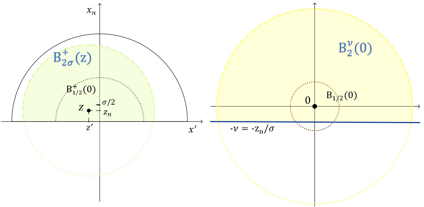
Figure 1: Illustration of the change of variable, from $B^{+}_{2\sigma}(z)=B_{2\sigma}(z)\cap\{x_{n}>0\}$, which is a subset of $B_{1}^{+}(0)$, to $B_{2}^{\nu}(0)=B_{2}(0)\cap\{x_{n}>-\nu\}$.

Then we define $N=N_{\sigma}(z):=\sigma W+\sup_{x\in B_{2}^{\nu}(0)}|u(\sigma x+z)-u(z)|.$ The $C^{\beta}$ quadratic estimate, this time the global one, restricted to the set $B_{2\sigma}^{+}(z)$, yields

$$\sigma W\leq N\leq(\sigma+2^{\beta}K_{1}\sigma^{\beta})W\leq(1+2^{\beta}K_{1})\sigma^{\beta}W_{0}.$$ (3.12)

Next we set $\widetilde{u}(x)=\frac{1}{N}\{u(\sigma x+z)-u(z)\}$, which is, as in claim 3.2, an $L^{p}$-viscosity solution of

$$\left\{\begin{array}[]{rclcc}\widetilde{F}(x,\widetilde{u},D\widetilde{u},D^{2}\widetilde{u})&=&\widetilde{f}(x)&\mbox{in}&B_{2}^{\nu}\\ \widetilde{u}&=&\widetilde{\psi}&\textrm{on}&\mathbb{T}^{\nu}_{2}\end{array}\right.$$

for

$$\widetilde{F}(x,r,p,X):=\frac{\sigma^{2}}{N}F\left(\sigma x+z,Nr+u(z),\frac{N}{\sigma}p,\frac{N}{\sigma^{2}}X\right)-\frac{\sigma^{2}}{N}F(\sigma x+z,u(z),0,0),$$

$\widetilde{\psi}(x):=\frac{1}{N}\{\psi(\sigma x+z)-u(z)\}$ and $\widetilde{f}:=\widetilde{f}_{1}+\widetilde{f}_{2}$ where

$$\widetilde{f}_{1}(x):={\sigma^{2}}f(\sigma x+z)/{N};\;\;\widetilde{f}_{2}(x):=-{\sigma^{2}}F(\sigma x+z,u(z),0,0)/{N},$$

$\widetilde{F}$ satisfying $(\widetilde{SC})^{\widetilde{\mu}}$ for $\widetilde{b}(x)=\sigma b(\sigma x+z)$, $\widetilde{\mu}=N\mu$, $\widetilde{d}(x)=\sigma^{2}d(\sigma x+z)$ and $\widetilde{\omega}(r)=\omega(Nr)/N$.

With this definition and the choice of $\sigma$ in (3.5), we obtain $\|\widetilde{u}\|_{L^{\infty}(B_{2}^{\nu})}\leq 1$, $\|\widetilde{f}\|_{L^{p}(B_{2}^{\nu})}\leq\frac{\delta}{8}$, $\widetilde{\mu}\leq\frac{\delta}{8K^{2}|B_{1}|^{1/p}}$, $\|\widetilde{b}\|_{L^{p}(B_{2}^{\nu})}\leq\frac{\delta}{16K}$, $\widetilde{\omega}(1)\|\widetilde{d}\|_{L^{p}(B_{2}^{\nu})}\leq\frac{\delta}{32(K_{4}+K+1)}$ and $\|\bar{\beta}_{\widetilde{F}}(0,\cdot)\|_{L^{p}(B_{1}^{\nu})}\leq\delta/4$ by choosing $\theta=\delta/8$, as in the local case.

Furthermore, we have $\|\widetilde{\psi}\|_{L^{\infty}(\mathbb{T}^{\nu}_{2})}\leq\|\widetilde{u}\|_{L^{\infty}(B_{2}^{\nu})}\leq 1$ and then $\|D\widetilde{\psi}\|_{C^{\tau}(\mathbb{T}^{\nu}_{2})}$ is bounded by

$$\frac{\sigma}{N}\|D\psi\|_{L^{\infty}(B_{2\sigma}(z)\cap\mathbb{T})}+\frac{\sigma}{N}\sup_{\begin{subarray}{c}x\neq y\in\mathbb{T}_{2}^{\nu}\end{subarray}}\frac{|D\psi(\sigma x+z)-D\psi(\sigma y+z)|}{|\sigma x-\sigma y|^{\tau}}\sigma^{\tau}\leq\frac{\|\psi\|_{C^{1,\tau}(\mathbb{T})}}{W}\leq 1$$

since $N\geq\sigma W$. Therefore, we obtain $\|\widetilde{\psi}\|_{C^{1,\tau}(\mathbb{T}^{\nu}_{2})}=\|\widetilde{\psi}\|_{L^{\infty}(\mathbb{T}^{\nu}_{2})}+\|D\widetilde{\psi}(x)\|_{C^{\tau}(\mathbb{T}^{\nu}_{2})}\leq 2$.

We can suppose, up to this rescaling, that $F,u,\mu,b,d,\omega$ satisfy the former hypotheses related to $\widetilde{F},\widetilde{u},\widetilde{\mu},\widetilde{b},\widetilde{d},\widetilde{\omega}$. Thus, we move to the construction of $l_{k}(x):=a_{k}+b_{k}\cdot x$ such that

$(i)_{k}\;\;\|u-l_{k}\|_{L^{\infty}(B_{r_{k}}^{\nu})}\leq r_{k}^{1+\alpha}$

$(ii)_{k}\;\;|a_{k}-a_{k-1}|\leq K_{4}\,r_{k-1}^{1+\alpha}\;,\;\;|b_{k}-b_{k-1}|\leq K_{4}\,r_{k-1}^{\alpha}$

$(iii)_{k}\;\;|(u-l_{k})(r_{k}x)-(u-l_{k})(r_{k}y)|\leq C_{1,4}\,r_{k}^{1+\alpha}|x-y|^{\beta}\;\;\textrm{ for all }x,y\in B_{1}^{\nu_{k}}$
where $C_{1,4}=C_{1,4}\,(K_{1},K_{4})$ and $\nu_{k}:=\frac{\nu}{r_{k}}$, $r_{k}=\gamma^{k}$ for some $\gamma\in(0,1)$, for all $k\geq 0$ ($l_{-1}\equiv 0$).

We emphasize that these iterations will prove that the function $u$ (which plays the role of $\widetilde{u}$) is differentiable at $0$ and provide $|u(x)-u(0)-Du(0)\cdot x|\leq C|x|^{1+\alpha}$, $|Du(0)|\leq C$ for every $x\in B_{1}^{\nu}$. In terms of our original function defined on $B_{1}^{+}$, it means that $u$ will be differentiable at $z$, for all $z$ with $z_{n}<\frac{\sigma}{2}$. On the other hand, the second case $z_{n}\geq\frac{\sigma}{2}$ is covered by the local part, section 3.1, since in this situation we are far away from the bottom boundary. Consequently, boundary superlinear regularity and estimates on $B_{1}^{+}$ will follow by a covering argument.

For the proof of $(i)_{k}-(iii)_{k}$, we use induction on $k$. For $k=0$ we set $a_{0}=b_{0}=0$. Recall that $\beta$ and $K_{1}$ are the constants from $C^{\beta}$ quadratic global estimate in the set $B_{1}^{\nu}$, then we have $\|u\|_{C^{\beta}(\overline{B_{1}^{\nu}})}\leq\widetilde{K}_{1}(1+\delta+2+1)\leq 5K_{1}$ and so $(iii)_{0}$ for $\nu_{0}=\nu$, $(i)_{0}$ and $(ii)_{0}$ are valid.

Analogously to the the local case, we have $|b_{k}|,\;\|l_{k}\|_{L^{\infty}(B_{r_{k}}^{\nu})}\leq K.$ For the induction’s step we suppose $(i)_{k}-(iii)_{k}$ and construct $a_{k+1}$, $b_{k+1}$ such that $(i)_{k+1}-(iii)_{k+1}$ are valid. Define

$$v(x)=v_{k}({x}):=\frac{(u-l_{k})(r_{k}{x})}{r_{k}^{1+\alpha}}=\frac{u(r_{k}{x})-a_{k}-b_{k}\cdot xr_{k}}{r_{k}^{1+\alpha}}\,,\;\textrm{ for all }\,{x}\in B_{2}^{\nu_{k}}.$$

Since $r_{k}x\in B_{r_{k}}^{\nu}\Leftrightarrow x\in B_{1}^{\nu_{k}}$, $(i)_{k}$ says that $|v|\leq 1$ in $B_{1}^{\nu_{k}}.$ From this and $(iii)_{k}$, we get

$$\|v\|_{C^{\beta}(\overline{B_{1}^{\nu_{k}}})}=\|v\|_{L^{\infty}({B}_{1}^{\nu_{k}})}+\sup_{\begin{subarray}{c}x,y\in B_{1}^{\nu_{k}}\\ x\neq y\end{subarray}}\frac{|v(x)-v(y)|}{|x-y|^{\beta}}\leq 1+C_{1,4}=:K_{0}.$$

Notice that, as in the local case, it follows from claim 3.5 that $v$ is as an $L^{p}$-viscosity solution of

$$\left\{\begin{array}[]{rclcc}F_{k}(x,v+L_{k}(x),Dv+B_{k},D^{2}v)&=&f_{k}(x)&\mathrm{in}&B_{2}^{\nu_{k}}\\ v&=&\psi_{k}&\mathrm{on}&\mathbb{T}_{2}^{\nu_{k}}\end{array}\right.$$

where $f_{k}(x):=r_{k}^{1-\alpha}f(r_{k}x)$, $L_{k}(x)=A_{k}+B_{k}\cdot x$ in $B_{2}^{\nu_{k}}$ for $A_{k}=r_{k}^{-1-\alpha}a_{k}$, $B_{k}=r_{k}^{-\alpha}b_{k}$, and

$$F_{k}(x,s,p,X):=r_{k}^{1-\alpha}F(r_{k}x,r_{k}^{1+\alpha}s,r_{k}^{\alpha}p,r_{k}^{\alpha-1}X)$$

satisfying $(SC)_{F_{k}}^{\mu_{F_{k}}}$ for $b_{F_{k}}(x)=r_{k}b(r_{k}x)$, $\mu_{F_{k}}=r_{k}^{1+\alpha}\mu$, $d_{F_{k}}(x)=r_{k}^{2}d(r_{k}x)$, and $\omega_{F_{k}}(s)=r_{k}^{-1-\alpha}\omega(r_{k}^{1+\alpha}s)$, for the Lipschitz modulus $\omega$.

The above coefficients satisfy the hypotheses of lemma 3.7, since $\|b_{F_{k}}\|_{L^{p}(B_{1}^{\nu_{k}})}(|B_{k}|+1)\leq\delta$, $\mu_{F_{k}}(|B_{k}|^{2}+|B_{k}|+1)\leq\delta$, $\omega_{F_{k}}(1)\|d_{F_{k}}\|_{L^{p}(B_{1}^{\nu_{k}})}(|A_{k}|+|B_{k}|+1)\leq\delta$, $\|v\|_{\infty}\leq 1$, $\|f_{k}\|_{L^{p}(B_{1}^{\nu_{k}})}\leq\delta$, and $\|\bar{\beta}_{F_{k}}(\cdot,0)\|_{L^{p}(B_{1}^{\nu_{k}})}\leq\delta$, see section 3.1.

Let $h=h_{k}\in C(\overline{B_{1}^{\nu_{k}}})$ be the $C$-viscosity solution of

$$\left\{\begin{array}[]{rclcc}F_{k}(0,0,0,D^{2}h)&=&0&\mbox{in}&B_{1}^{\nu_{k}}\\ h&=&v&\mbox{on}&\partial B_{1}^{\nu_{k}}\end{array}\right.$$

given by proposition 2.10, since $B_{1}^{\nu_{k}}$ has the uniform exterior cone condition. From ABP we get $\|h\|_{L^{\infty}(B_{1}^{\nu_{k}})}\leq\|h\|_{L^{\infty}(\partial B_{1}^{\nu_{k}})}\leq 1$. Further, $h=v=\psi_{k}\in C^{1,\tau}(B_{1}\cap\{x_{n}=-\nu_{k}\})$ and we can find a uniform bound for the $C^{1,\tau}$ norm of $\psi_{k}$. Indeed, $\|\psi_{k}\|_{L^{\infty}(\mathbb{T}_{1}^{\nu_{k}})}\leq\|v\|_{L^{\infty}(\overline{B_{1}^{\nu_{k}}})}\leq 1$ and

$$[D\psi_{k}]_{\tau,\mathbb{T}_{1}^{\nu_{k}}}=\sup_{\begin{subarray}{c}x,y\in\mathbb{T}_{1}^{\nu_{k}}\\ x\neq y\end{subarray}}\frac{|D\psi_{k}(x)-D\psi_{k}(y)|}{|x-y|^{\tau}}=\sup_{\begin{subarray}{c}\tilde{x},\tilde{y}\in\mathbb{T}_{r_{k}}^{\nu}\\ \tilde{x}=r_{k}x,\,\tilde{y}=r_{k}y\end{subarray}}\frac{|D\psi(\tilde{x})-D\psi(\tilde{y})|}{|\tilde{x}-\tilde{y}|^{\tau}}r_{k}^{\tau-\alpha}\leq 1$$

since $\|D\psi\|_{C^{\tau}(\mathbb{T}_{1}^{\nu})}\leq 1$ and $\alpha\leq\tau$. Moreover, using the global Holder interpolation in smooth domains, lemma 6.35 of [20], for $\epsilon=\frac{1}{2}$, there exists a constant $C_{n}$ such that

$$\|\psi_{k}\|_{C^{1}(\mathbb{T}_{1}^{\nu_{k}})}\leq C_{n}\,\|\psi_{k}\|_{C(\mathbb{T}_{1}^{\nu_{k}})}+\frac{1}{2}\|\psi_{k}\|_{C^{1,\tau}(\mathbb{T}_{1}^{\nu_{k}})}$$

hence

$$\|\psi_{k}\|_{C^{1,\tau}(\mathbb{T}_{1}^{\nu_{k}})}=\|\psi_{k}\|_{C^{1}(\mathbb{T}_{1}^{\nu_{k}})}+[D\psi_{k}]_{\tau,\mathbb{T}_{1}^{\nu_{k}}}\leq C_{n}+\frac{1}{2}\|\psi_{k}\|_{C^{1,\tau}(\mathbb{T}_{1}^{\nu_{k}})}+1$$

i.e. $\|\psi_{k}\|_{C^{1,\tau}(\mathbb{T}_{1}^{\nu_{k}})}\leq 2(C_{n}+1)$. Thus, the $C^{1,\bar{\alpha}}$ global estimate (proposition 2.11) yields

$$\|h\|_{C^{1,\bar{\alpha}}(\overline{B_{1/2}^{\nu_{k}}})}\leq K_{3}\,\{\|h\|_{L^{\infty}(B_{1}^{\nu_{k}})}+\|\psi_{k}\|_{C^{1,\tau}(\mathbb{T}_{1}^{\nu_{k}})}\}\leq K_{3}\,(3+2C_{n})=:K_{4}.$$

Now, the approximation boundary lemma 3.1 applied to $F_{k},v,h,\nu_{k},\mu_{F_{k}},b_{F_{k}},d_{F_{k}},\omega_{F_{k}},A_{k},B_{k},\psi_{k}$, $\beta,K_{0}$ gives us that $\|v-h\|_{L^{\infty}(B_{1}^{\nu_{k}})}\leq\varepsilon.$

Therefore, defining $\overline{l}(x)=\overline{l}_{k}(x):=h(0)+Dh(0)\cdot x$ in $B_{1}^{\nu_{k}}$, we have

$$\|v-\overline{l}\|_{L^{\infty}(B_{2\gamma}^{\nu_{k}})}\leq\gamma^{1+\alpha}.$$ (3.13)

In fact, by the choice of $\gamma$ we have, for all $x\in B_{2\gamma}^{\nu_{k}}(0)$,

$$|v(x)-\overline{l}(x)|\leq|v(x)-h(x)|+|h(x)-h(0)-Dh(0)\cdot x|\leq 2K_{4}\,(2\gamma)^{1+\bar{\alpha}}\leq\gamma^{1+\alpha}.$$

Next, (3.13) and the definition of $v$ imply

$$|u(r_{k}{x})-l_{k}(r_{k}x)-r_{k}^{1+\alpha}h(0)-r_{k}^{1+\alpha}Dh(0)\cdot x|\leq r_{k}^{1+\alpha}\gamma^{1+\alpha}=r_{k+1}^{1+\alpha}\,\;\textrm{ for all }x\in B_{2\gamma}^{\nu_{k}}\,,$$

which is equivalent to

$$|u(y)-l_{k+1}(y)|\leq r_{k}^{1+\alpha}\gamma^{1+\alpha}=r_{k+1}^{1+\alpha}\,\;\textrm{ for all }y=r_{k}x\in B_{2\gamma r_{k}}^{\nu}=B_{2r_{k+1}}^{\nu}\,,$$

where $l_{k+1}(y):=l_{k}(y)+r_{k}^{1+\alpha}h(0)+r_{k}^{\alpha}Dh(0)\cdot y$. Then, we define $a_{k+1}:=a_{k}+h(0)r_{k}^{1+\alpha}$, $b_{k+1}:=b_{k}+Dh(0)r_{k}^{\alpha}$, obtaining $(i)_{k+1}$. Also, $|a_{k+1}-a_{k}|\leq K_{4}\,r_{k}^{1+\alpha}$, $|b_{k+1}-b_{k}|\leq K_{4}\,r_{k}^{\alpha}$, which is $(ii)_{k+1}$. As in the local case, to finish the proof of $(iii)_{k+1}$, it is enough to show that

$$\|v-\overline{l}\|_{C^{\beta}(\overline{B_{\gamma}^{\nu_{k}}})}\leq C_{1,4}\,\gamma^{1+\alpha-\beta}.$$

Let us see that this is obtained by applying the global superlinear $C^{\beta}$ estimate in proposition 2.6 to the function $w:=v-\overline{l}$.

Analogously to the local case, $w$ is an $L^{p}$-viscosity solution in $B_{2}^{\nu_{k}}$ of (3.10) (see notations and coefficients there), in addition to $w=\psi_{k}-\overline{l}$ on $\mathbb{T}_{2}^{\nu_{k}}$. The definition of $\delta$ gives us $\|g_{k}\|_{L^{p}(B_{1}^{\nu_{k}})}\leq(5+2K_{4})\delta\leq\gamma^{\alpha}$. Further, using that $\psi_{k}=h$ on $\mathbb{T}_{2\gamma}^{\nu_{k}}$, we obtain $\|\psi_{k}-\overline{l}\|_{L^{\infty}(\mathbb{T}_{2\gamma}^{\nu_{k}})}\leq\gamma^{1+{\alpha}}.$

Now, since $\psi_{k}-\overline{l}\in C^{1}(\mathbb{T}_{2\gamma}^{\nu_{k}})$, it is a Lipschitz function with constant less or equal than $\|D\psi_{k}-D\overline{l}\,\|_{C(\mathbb{T}_{2\gamma}^{\nu_{k}})}\leq 2(C_{n}+1)+K_{4}\leq 2K_{4}$ and thus

$$|(\psi_{k}-\overline{l})(x)-(\psi_{k}-\overline{l})(y)| =|(\psi_{k}-\overline{l})(x)-(\psi_{k}-\overline{l})(y)|^{\tau}|(\psi_{k}-\overline{l})(x)-(\psi_{k}-\overline{l})(y)|^{1-\tau}$$

$$\leq(2K_{4})^{\tau}(2K_{4})^{1-\tau}|x-y|^{\tau}\,\gamma^{(1+\bar{\alpha})(1-\tau)}=2K_{4}\,|x-y|^{\tau}\,\gamma^{1-\tau+\bar{\alpha}(1-\tau)}.$$

Then, the choice of $\alpha$ implies that $[\psi_{k}-\overline{l}]_{\tau,\mathbb{T}_{2\gamma}^{\nu_{k}}}\leq 4K_{4}\,\gamma^{1-\tau+\alpha}.$ Hence, from this, (3.13) and $C^{\beta}$ global estimate, properly scaled for the radius $\gamma$, we obtain

$$[w]_{\beta,\overline{B_{\gamma}^{\nu_{k}}}} \leq\gamma^{-\beta}\widetilde{K}_{1}\,\{\,\|w\|_{L^{\infty}({B_{2\gamma}^{\nu_{k}}})}+\gamma^{2-\frac{n}{p}}\|g_{k}\|_{L^{p}({B_{2\gamma}^{\nu_{k}}})}+\|\psi_{k}-\overline{l}\|_{L^{\infty}(\mathbb{T}_{2\gamma}^{\nu_{k}})}+\gamma^{\tau}[\psi_{k}-\overline{l}]_{\tau,\mathbb{T}_{2\gamma}^{\nu_{k}}}\,\}$$

$$\leq\gamma^{-\beta}K_{1}\,\{\,2\gamma^{1+\alpha}+\gamma^{2-\frac{n}{p}}\gamma^{\alpha}+4K_{4}\,\gamma^{1+\alpha}\,\}\leq K_{1}\,(3+4K_{4})\,\gamma^{1+\alpha-\beta}$$

and finally, for $C_{1,4}:=1+(3+4K_{4})K_{1}=C_{1,4}\,(K_{1},K_{4})$, we conclude

$$\|w\|_{C^{\beta}(\overline{B_{\gamma}^{\nu_{k}}})}=\|w\|_{L^{\infty}({B_{\gamma}^{\nu_{k}}})}+[w]_{\beta,\overline{B_{\gamma}^{\nu_{k}}}}\leq\gamma^{1+\alpha}+(3+4K_{4})K_{1}\,\gamma^{1+\alpha-\beta}\leq C_{1,4}\,\gamma^{1+\alpha-\beta}.$$

∎

Therefore, the complete proof of regularity and estimates in the global case is done by a covering argument over the domain $\Omega$, using local and boundary results.

4 $W^{2,p}$ Results

The first application of the $C^{1,\alpha}$ theory is $W^{2,p}$ regularity for solutions of fully nonlinear equations with superlinear growth in the gradient, which are convex or concave in the variable $X$. This extends the results in [56] to superlinear growth in the gradient in the case $p>n$.

In the next two sections we make the convention that $\omega$ is a Lipschitz modulus in the sense that $\omega(r)\leq\omega(1)r$, for all $r\geq 0$, unless otherwise specified.

Theorem 4.1.

$(W^{2,p}$ Regularity $)$ Let $\Omega\subset{\mathbb{R}^{n}}$ be a bounded domain and $u\in C(\Omega)$ an $L^{p}$-viscosity solution of

$$F(x,u,Du,D^{2}u)+g(x,Du)=f(x)\quad\textrm{in}\;\;\;\Omega$$ (4.1)

where $f\in L^{p}(\Omega)$, $p>n$, $g$ is a measurable function in $x$ such that $g(x,0)=0$ and $|g(x,p)-g(x,q)|\leq\gamma|p-q|+\mu|p-q|(|p|+|q|)$, $F$ is convex or concave in $X$ satisfying $(SC)^{0}$, for $b,\,d\in L^{\infty}_{+}(\Omega)$ and $\omega$ a Lipschitz modulus. Also, suppose $\|u\|_{L^{\infty}(\Omega)}+\|f\|_{L^{p}(\Omega)}\leq C_{0}$. Then, there exists $\theta=\theta(n,p,\lambda,\Lambda,\|b\|_{L^{p}(\Omega)})$ such that, if ($H_{\theta}$) holds for all $r\leq\min\{r_{0},\mathrm{dist}(x_{0},\partial\Omega)\}$, for some $r_{0}>0$ and for all $x_{0}\in\Omega$, this implies that $u\in W^{2,p}_{\mathrm{loc}}(\Omega)$ and for every $\Omega^{\prime}\subset\subset\Omega$,

$$\|u\|_{W^{2,p}(\Omega^{\prime})}\leq C\,\{\|u\|_{L^{\infty}(\Omega)}+\|f\|_{L^{p}(\Omega)}\}$$

where $C$ depends on $\,r_{0},n,p,\lambda,\Lambda,\mu,\|b\|_{L^{p}(\Omega)},\omega(1)\|d\|_{L^{\infty}(\Omega)},\mathrm{dist}(\Omega^{\prime},\partial\Omega),\mathrm{diam}(\Omega)$ and $C_{0}$.

If, moreover, $\partial\Omega\in C^{1,1}$, $u\in C(\overline{\Omega})$ and $u=\psi$ on $\partial\Omega$ for some $\psi\in W^{2,p}(\Omega)$ with $\|u\|_{L^{\infty}(\Omega)}+\|f\|_{L^{p}(\Omega)}+\|\psi\|_{W^{2,p}(\Omega)}\leq C_{1}$ then, there exists $\theta=\theta(n,p,\lambda,\Lambda,\|b\|_{L^{p}(\Omega)})$ such that, if ($H_{\theta}$) holds for some $r_{0}>0$ and for all $x_{0}\in\overline{\Omega}$, this implies that $u\in W^{2,p}(\Omega)$ and satisfies the estimate

$$\|u\|_{W^{2,p}(\Omega)}\leq C\,\{\|u\|_{L^{\infty}(\Omega)}+\|f\|_{L^{p}(\Omega)}+\|\psi\|_{W^{2,p}(\Omega)}\}$$

where $C$ depends on $r_{0},n,p,\lambda,\Lambda,\mu,\|b\|_{L^{p}(\Omega)},\omega(1)\|d\|_{L^{\infty}(\Omega)},\partial\Omega,\mathrm{diam}(\Omega)$ and $C_{1}$.

Proof.

We prove only the global case, since in the local one we just ignore the term with $\psi$, by considering it equal to zero in what follows. Notice that $\psi\in W^{2,p}(\Omega)\subset C^{1,\tau}(\overline{\Omega})$ for some $\tau\in(0,1)$ with continuous inclusion, then $\|u\|_{L^{\infty}(\Omega)}+\|f\|_{L^{p}(\Omega)}+\|\psi\|_{C^{1,\tau}(\partial\Omega)}\leq C_{2}$.

Thus, by $C^{1,\alpha}$ regularity theorem, we have that $\bar{f}(x):=f(x)-g(x,Du)\in L^{p}(\Omega)$ and also

$$\|u\|_{C^{1,\alpha}(\overline{\Omega})}\leq C_{3}\,\{\|u\|_{L^{\infty}(\Omega)}+\|\bar{f}\|_{L^{p}(\Omega)}+\|\psi\|_{C^{1,\tau}(\partial\Omega)}\}.$$

Claim 4.2.

$u$ is an $L^{p}$-viscosity solution of $F(x,u,Du,D^{2}u)=\bar{f}(x)$ in $\Omega$.

Proof.

Let us prove the subsolution case; for the supersolution it is analogous. Assuming the contrary, there exists some $\phi\in W^{2,p}_{\mathrm{loc}}(\Omega)$, $x_{0}\in\Omega$ and $\varepsilon>0$ such that $u-\phi$ has a local maximum at $x_{0}$ and $F(x,u,D\phi,D^{2}\phi)-\bar{f}(x)\leq-\varepsilon$  a.e. in $B_{r}(x_{0})$.

In turn, by the definition of $u$ being an $L^{p}$-viscosity subsolution of (4.1), we have that

$F(x,u,D\phi,D^{2}\phi)+g(x,D\phi)\geq f(x)-\varepsilon/2$  a.e. in $B_{r}(x_{0})$

up to diminishing $r>0$. By subtracting the last two inequalities, we obtain that

$$-\{\gamma+\mu(|Du|+|D\phi|)\}\,|Du-D\phi|\leq g(x,Du)-g(x,D\varphi)\leq-\varepsilon/2\,\textrm{ a.e. in }B_{r}(x_{0}).$$ (4.2)

Since $u-\phi\in C^{1}(B_{r}(x_{0}))$ has a local maximum at $x_{0}$, we have $D(u-\phi)(x_{0})=0$ and, moreover, $|D(u-\phi)(x)|<\varepsilon\,\{\gamma+\mu(\|Du\|_{L^{\infty}(B_{r}(x_{0}))}+\|D\phi\|_{L^{\infty}(B_{r}(x_{0})})+1\}^{-1}/4\,$ for all $x\in B_{r}(x_{0})$, possibly for a smaller $r$, which contradicts (4.2). ∎Claim 4.2.

Thus by Winter’s result, theorem 4.3 in [56] (or Świech [50] in the local case), we have that $u\in W^{2,p}(\Omega)$ (respectively $u\in W^{2,p}_{\mathrm{loc}}(\Omega)$) and

$$\|u\|_{W^{2,p}(\Omega)}\leq C\,\{\|u\|_{L^{\infty}(\Omega)}+\|\bar{f}\|_{L^{p}(\Omega)}+\|\psi\|_{W^{2,p}(\Omega)}\}$$

$$\leq C\,\{\|u\|_{L^{\infty}(\Omega)}+\|f\|_{L^{p}(\Omega)}+\mu\|u\|_{C^{1}(\overline{\Omega})}^{2}+\gamma\|u\|_{C^{1}(\overline{\Omega})}+\|\psi\|_{W^{2,p}(\Omega)}\}$$

$$\leq C\,\{\|u\|_{L^{\infty}(\Omega)}+\|f\|_{L^{p}(\Omega)}+\|\psi\|_{W^{2,p}(\Omega)}+(\mu\,C_{2}+\gamma)C_{3}\{\|u\|_{L^{\infty}(\Omega)}+\|f\|_{L^{p}(\Omega)}+\|\psi\|_{C^{1,\tau}(\partial\Omega)}\}\}$$

which implies the estimate. ∎

In theorem 4.1, the final constants only depend on the $L^{p}$-norm of the coefficient $b$, despite the boundedness hypothesis on it. The latter hypothesis is needed to conclude that solutions are twice differentiable a.e. Observe that, in [56] (see theorem 4.3 there), $W^{2,p}$ results consist of two parts: (i) introducing a new equation $F(x,0,0,D^{2}u)=\tilde{f}(x)$ (via corollary 1.6 in [50]), in which $u$ remains a solution in the $L^{p}$-viscosity sense; (ii) obtaining $W^{2,p}$ estimates for solutions of $F(x,0,0,D^{2}u)=\widetilde{f}(x)$, which are independent of the zero and first order coefficients.

From the regularity and estimates related to $\mu=0$, we can give an alternative proof of proposition 2.4 in [32], concerning existence and uniqueness for the Pucci’s extremal operators with unbounded coefficients in the case $p>n$.

Proposition 4.3.

$($Solvability of the Dirichlet problem $)$ Let $\Omega\subset{\mathbb{R}^{n}}$ be a bounded $C^{1,1}$ domain. Let $b,\,d\in L^{p}_{+}(\Omega)$, $p>n$ and $\omega$ a Lipschitz modulus. Let $f\in L^{p}(\Omega)$ and $\psi\in W^{2,p}(\Omega)$. Then, there exists $u_{\pm}\in C(\overline{\Omega})$ which are the unique $L^{p}$-viscosity solutions of the problems

$$\left\{\begin{array}[]{rllll}\mathcal{M}^{\pm}_{\lambda,\Lambda}(D^{2}u_{\pm})\pm b(x)|Du_{\pm}|\pm d(x)w((\mp\,u_{\pm})^{+})&=&f(x)&\mbox{in}&\Omega\\ u_{\pm}&=&\psi&\mbox{on}&\partial\Omega\,.\end{array}\right.$$

Moreover, $u_{\pm}\in W^{2,p}(\Omega)$ and satisfies the estimate

$$\|u_{\pm}\|_{W^{2,p}(\Omega)}\leq C\,\{\|u_{\pm}\|_{L^{\infty}(\Omega)}+\|f\|_{L^{p}(\Omega)}+\|\psi\|_{W^{2,p}(\Omega)}\}$$

where $C$ depends only on $n,p,\lambda,\Lambda,\|b\|_{L^{p}(\Omega)},\omega(1)\,\|d\|_{L^{p}(\Omega)},\partial\Omega$ and $\mathrm{diam}(\Omega)$.

Proof.

It is enough to treat the upper extremal case. Let $b_{k},\,d_{k}\in L^{\infty}_{+}(\Omega)$ be such that $b_{k}\rightarrow b$ and $d_{k}\rightarrow d$ in $L^{p}(\Omega)$. Let $u_{k}\in W^{2,p}(\Omega)$ be the unique $L^{p}$-viscosity solution of

$$\left\{\begin{array}[]{rllll}\mathcal{M}^{+}_{\lambda,\Lambda}(D^{2}u_{k})+b_{k}(x)|Du_{k}|+d_{k}(x)\,\omega(u_{k}^{-})&=&f(x)&\mbox{in}&\Omega\\ u_{k}&=&\psi&\mbox{on}&\partial\Omega\end{array}\right.$$

given by theorem 4.6 of [56]. From the estimates in theorem 4.1, with $d_{k}(x)\omega(u_{k}^{-})$ as RHS,

$$\|u_{k}\|_{W^{2,p}(\Omega)}\leq C_{k}\,\{\|u_{k}\|_{L^{\infty}(\Omega)}+\|f\|_{L^{p}(\Omega)}+\|\psi\|_{W^{2,p}(\Omega)}\},$$ (4.3)

where $C_{k}$ remains bounded, since $b_{k}$ and $d_{k}$ are bounded in $L^{p}(\Omega)$.

Now, by ABP we have that that $\|u_{k}\|_{L^{\infty}(\Omega)}\leq\|\psi\|_{L^{\infty}(\partial\Omega)}+C\,\|f\|_{L^{p}(\Omega)}$. From this and (4.3) we get $\|u_{k}\|_{W^{2,p}(\Omega)}\leq C$ and hence there exists $u\in C^{1}(\overline{\Omega})$ such that $u_{k}\rightarrow u$ in $C^{1}(\overline{\Omega})$.

Next, proposition 2.3 implies that $u$ is an $L^{p}$-viscosity solution of

$$\left\{\begin{array}[]{rllll}\mathcal{M}^{+}_{\lambda,\Lambda}(D^{2}u)+b(x)|Du|+d(x)\,\omega(u^{-})&=&f(x)&\mbox{in}&\Omega\\ u&=&\psi&\mbox{on}&\partial\Omega\,.\end{array}\right.$$ (4.6)

Notice that $W^{2,p}(\Omega)$ is reflexive, so there exists $\tilde{u}\in W^{2,p}(\Omega)$ such that $u_{k}$ converges weakly to $\tilde{u}$. By uniqueness of the limit, $\tilde{u}=u$ a.e. in $\Omega$, and $u$ is a strong solution of (4.6).

Finally, if there would exist another $L^{p}$-viscosity solution of (4.6), say $v\in C(\overline{\Omega})$, then the function $w:=u-v$ satisfies $w=0$ on $\partial\Omega$ and it is an $L^{p}$-viscosity solution of $\mathcal{L}^{+}[w]\geq 0$ in $\Omega\cap\{w>0\}$. Indeed, since $u$ is strong, we can apply the definition of $v$ as an $L^{p}$-viscosity supersolution with $u$ as a test function; we also use that $u^{-}\leq v^{-}+(u-v)^{-}$, monotonicity and subadditivity of the modulus. Then, by ABP we have that $w\leq 0$ in $\Omega$. Analogously, from the definition of subsolution of $v$, we obtain $w\geq 0$ in $\Omega$, and so $w\equiv 0$ in $\Omega$. ∎

The approximation procedure in the above proof cannot be used to extend theorem 4.1 for unbounded $b$ and $d$, since in this case we do not have uniqueness results to infer that the limiting function is the same as the one we had started with. However, knowing a priori that the solution is strong, we can obtain $W^{2,p}$ a priori estimates in the general case, as a kind of generalization of Nagumo’s lemma (for instance, lemma 5.10 in [51]).

Lemma 4.4.

$($Generalized Nagumo’s lemma $)$ Let $\Omega\subset{\mathbb{R}^{n}}$ be a bounded $C^{1,1}$ domain. Let $F$ be a convex or concave operator in the $X$ entry, satisfying 1, with $b,\,d\in L^{p}_{+}(\Omega)$ for $p>n$ and $\omega$ an arbitrary modulus. Suppose that there exists $\theta>0$ such that ($H_{\theta}$) holds for some $r_{0}>0$ and for all $x_{0}\in\overline{\Omega}$. Let $f\in L^{p}(\Omega)$, $\psi\in W^{2,p}(\Omega)$ and let $u\in W^{2,p}(\Omega)$ be a strong solution of

$$\left\{\begin{array}[]{rllll}F(x,u,Du,D^{2}u)&=&f(x)&\mbox{in}&\Omega\\ u&=&\psi&\mbox{on}&\partial\Omega\end{array}\right.$$

such that $\|u\|_{L^{\infty}(\Omega)}+\|f\|_{L^{p}(\Omega)}+\|\psi\|_{W^{2,p}(\Omega)}\leq C_{1}$. Then we have

$$\|u\|_{W^{2,p}(\Omega)}\leq C\,\{\|u\|_{L^{\infty}(\Omega)}+\|f\|_{L^{p}(\Omega)}+\|\psi\|_{W^{2,p}(\Omega)}+\|d\|_{L^{p}(\Omega)}\,\omega(\|u\|_{L^{\infty}(\Omega)})\}$$ (4.7)

where $C$ depends on $r_{0},n,p,\lambda,\Lambda,\mu,\|b\|_{L^{p}(\Omega)},C_{1},\partial\Omega$ and $\mathrm{diam}(\Omega)$. The local case is analogous.

If $\mu=0$, then the above constant $C$ does not depend on $C_{1}$.

Proof.

Note that, in particular, $u\in C^{1,\alpha}(\overline{\Omega})$ and satisfies $F(x,0,0,D^{2}u)=g(x)$ a.e. in $\Omega$, where

$$g(x):=f(x)-F(x,u,Du,D^{2}u)+F(x,0,0,D^{2}u)\in L^{p}(\Omega),$$

since $|F(x,u,Du,D^{2}u)-F(x,0,0,D^{2}u)|\leq b(x)|Du|+\mu|Du^{2}|+d(x)\,\omega(|u|)\in L^{p}(\Omega).$ Now, by theorem 4.1 (for $b,d,\mu,\gamma=0$) and the proof there dealing with $C^{1,\alpha}$ estimates,

$$\hskip 85.35826pt\|u\|_{W^{2,p}(\Omega)}\leq C\,\{\|u\|_{L^{\infty}(\Omega)}+\|g\|_{L^{p}(\Omega)}+\|\psi\|_{W^{2,p}(\Omega)}\}$$

$$\leq C\,\{\|u\|_{L^{\infty}(\Omega)}+\|f\|_{L^{p}(\Omega)}+\mu\|u\|_{C^{1}(\overline{\Omega})}^{2}+\|\psi\|_{W^{2,p}(\Omega)}+\|b\|_{L^{p}(\Omega)}\|u\|_{C^{1}(\overline{\Omega})}+\|d\|_{L^{p}(\Omega)}\,\omega(\|u\|_{\infty})\}$$

from where (4.7) follows. ∎

5 The weighted eigenvalue problem

We start recalling some notations.

A subset $K\subset E$ of a Banach space is an ordered cone if it is closed, convex, $\lambda K\subset K$ for all $\lambda\geq 0$ and $K\cap(-K)=\{0\}$. This cone induces a partial order on $E$, for $u,v\in E$, given by $u\leq v\Leftrightarrow v-u\in K.$ We say that $K$ is solid if $\mathrm{int}K\neq\emptyset$. Further, a completely continuous operator, defined in $E$, is continuous and takes bounded sets into precompact ones.

Following the construction of [2], [43], we have the following Krein-Rutman theorem for nonlinear operators – see [41].

Theorem 5.1.

$($Generalized Krein-Rutman $)$ Let $K\subset E$ be an ordered solid cone and let $T:K\rightarrow K$ be a completely continuous operator that is also

1. positively 1-homogeneous, i.e. $T(\lambda u)=\lambda Tu$, for all $\lambda\geq 0,u\in K$;

2. monotone increasing, i.e. for all $u,v\in K$, $u\leq v$ we have $Tu\leq Tv$;

3. strongly positive with respect to the cone, in the sense that $T(K\setminus\{0\})\subset\mathrm{int}K$.

Then $T$ has a positive eigenvalue $\alpha_{1}>0$ associated to a positive eigenfunction $w_{1}\in\mathrm{int}K$.

Consider $\Omega\subset{\mathbb{R}^{n}}$ a bounded $C^{1,1}$ domain. The application of Krein-Rutman is very standard for positive weights [2], [21]. Let us recall its use when we have a fully nonlinear operator with unbounded coefficients. About structure, we suppose

$$\mathcal{M}_{\lambda,\Lambda}^{-}(X-Y)-b(x)|p-q|-d(x)\,\omega((r-s)^{+})\leq F(x,r,p,X)-F(x,s,q,Y)$$ (SC)

$$\leq\mathcal{M}_{\lambda,\Lambda}^{+}(X-Y)+b(x)|p-q|+d(x)\,\omega((s-r)^{+})\;\;\textrm{ for }x\in\Omega$$

with $F(\cdot,0,0,0)\equiv 0$, where $0<\lambda\leq\Lambda$, $b\in L^{p}_{+}(\Omega)$, $p>n$, $d\in L^{\infty}_{+}(\Omega)$, $\omega$ a Lipschitz modulus. Here, the condition over the zero order term in (SC) means that $F$ is proper, i.e. decreasing in $r$.

Consider $E=C_{0}^{1}(\overline{\Omega})$ and the usual ordered solid cone $K=\{u\in E;\,u\geq 0\textrm{ in }\Omega\}$ in $E$.

Let $c(x)\in L^{p}_{+}(\Omega)$ with $c>0$ in $\overline{\Omega}$, $p>n$. As the operator on $K$, we take $T=-F^{-1}\circ c$ in the sense that $U=Tu$ iff $U$ is the unique $L^{n}$-viscosity solution of the Dirichlet problem

$$\left\{\begin{array}[]{rclcc}F(x,U,DU,D^{2}U)&=&-c(x)u&\mbox{in}&\Omega\\ U&=&0&\mbox{on}&\partial\Omega\end{array}\right.$$ (5.3)

where $F$ satisfies the following hypotheses

$$\left\{\begin{array}[]{l}\textrm{there exists }\theta>0\textrm{ such that }(\overline{H})_{\theta}\textrm{ holds for for all }x_{0}\in\overline{\Omega},\\ \eqref{SC}\textrm{ and }\eqref{ExistUnic T bem definido}\textrm{ hold},\;\,F(x,tr,tp,tX)=tF(x,r,p,X)\textrm{ for all }t\geq 0.\end{array}\right.$$ (5.6)

Here, hypothesis ($S$) means the solvability in $L^{n}$- sense with data in $L^{p}$, i.e. for any $f\in L^{p}(\Omega)$,

$$\textrm{there exists a unique }u\in C(\overline{\Omega})\;L^{n}\textrm{-viscosity solution of }F[u]=f(x)\textrm{ in }\Omega;\;u=0\textrm{ on }\partial\Omega. S$$ ()

Of course, Pucci’s extremal operators

$$\mathcal{L}^{\pm}[u]:=\mathcal{M}^{\pm}(D^{2}u)\pm b(x)|Du|\pm d(x)\omega(u^{\mp}),\;\;b,\,d\in L^{p}_{+}(\Omega),$$

where $\omega$ is a Lipschitz modulus, are particular examples of $F$ satisfying (5.6). Indeed, recall that proposition 4.3 provides a strong solution $u\in W^{2,p}(\Omega)\subset W^{2,n}(\Omega)$, which is an $L^{n}$-viscosity solution by proposition 2.2. Furthermore, since it is unique among $L^{p}$-viscosity solutions, it is also unique among $L^{n}$-viscosity ones. Here all the coefficients can be unbounded. Observe that ($S$) and $(\overline{H})_{\theta}$ also holds when $F$ is a uniformly continuous operator in $x$ satisfying the growth conditions in [1] (see also [27]), in this case concerning $C$-viscosity notions of solutions.

On the other hand, $(\overline{H})_{\theta}$, (SC) and ($S$) are completely enough to ensure existence, uniqueness and $C^{1,\alpha}$ global regularity and estimates for the problem 5.3 from Theorem 1.1, which in turn implies that the operator $T$ is well defined and completely continuous.

Furthermore, $T=-F^{-1}\circ c$ is strictly positive with respect to the cone, thanks to SMP and Hopf. In general, without the strict positiveness of $c$ in $\Omega$ there is no guarantee on this property, i.e., under $c\geq 0$ and $c\not\equiv 0$ in $\Omega$, we only obtain that $T(K\setminus\{0\})\subset K$.

Notice that $T=-F^{-1}\circ c\,$ has an eigenvalue $\alpha_{1}>0$ associated to the positive eigenfunction $\varphi_{1}$ if and only if $\varphi_{1}$ is an $L^{n}$-viscosity solution of

$$\left\{\begin{array}[]{rclcc}F[\varphi_{1}]+1/\alpha_{1}\,c(x)\varphi_{1}&=&0&\mbox{in}&\Omega\\ \varphi_{1}&>&0&\mbox{in}&\Omega\\ \varphi_{1}&=&0&\mbox{on}&\partial\Omega\,.\end{array}\right.$$

For any $c\in L^{p}(\Omega)$ with $p>n$ and $F$ satisfying (5.6), we can define, as in [5], [44],

$$\lambda_{1}^{\pm}=\lambda_{1}^{\pm}\,(F(c),\Omega) =\sup\left\{\lambda>0;\;\Psi^{\pm}(F(c),\Omega,\lambda)\neq\emptyset\right\}$$

where $\Psi^{\pm}(F(c),\Omega,\lambda):=\left\{\psi\in C(\overline{\Omega});\;\pm\psi>0\textrm{ in }\Omega,\;\pm(F[\psi]+\lambda c(x)\psi)\leq 0\textrm{ in }\Omega\right\}$; with inequalities holding in the $L^{n}$-viscosity sense. Notice that, by definition, $\lambda_{1}^{\pm}(G(c),\Omega)=\lambda_{1}^{\mp}(F(c),\Omega),$ where $G(x,r,p,X):=-F(x,-r,-p,-X)$.

With an approximation procedure by positive weights given by Krein-Rutman theorem as above, for $F$ satisfying (5.6), we obtain existence of eigenvalues with nonnegative weight.

Theorem 5.2.

Let $\Omega\subset{\mathbb{R}^{n}}$ be a bounded $C^{1,1}$ domain, $c\in L^{p}(\Omega)$, $c\gneqq 0$ for $p>n$ and $F$ satisfying (5.6) for $b,\,d\in L_{+}^{\infty}(\Omega)$. Then $F$ has two positive weighted eigenvalues $\alpha_{1}^{\pm}>0$ corresponding to normalized and signed eigenfunctions $\varphi_{1}^{\pm}\in C^{1,\alpha}(\overline{\Omega})$ that satisfies

$$\left\{\begin{array}[]{rclcc}F[\varphi_{1}^{\pm}]+\alpha_{1}^{\pm}c(x)\varphi_{1}^{\pm}&=&0&\mbox{in}&\Omega\\ \pm\varphi_{1}^{\pm}&>&0&\mbox{in}&\Omega\\ \varphi_{1}^{\pm}&=&0&\mbox{on}&\partial\Omega\end{array}\right.$$ (5.10)

in the $L^{p}$-viscosity sense, with $\max_{\overline{\Omega}}\,(\pm\varphi_{1}^{\pm})=1$.

If, moreover, the operator $F$ has $W^{2,p}$ regularity of solutions $($in the sense that every $u\in C(\overline{\Omega})$ which is an $L^{p}$-viscosity solution of $F[u]=f(x)\in L^{p}(\Omega)$, $u=0$ on $\partial\Omega$, satisfies $u\in W^{2,p}(\Omega))$, then $\alpha_{1}^{\pm}=\lambda^{\pm}_{1}$ and the conclusion is valid also for $b\in L^{p}_{+}(\Omega)$.

Notice that we obtain positive eigenvalues because $F$ is proper. For general existence related to nonproper operators see the script in [44] for bounded coefficients. We also stress that, without regularity assumptions on the domain, it is still possible to obtain the existence of an eigenpair, as in [5] and [44]; in such cases the eigenfunction belongs to $C^{1,\alpha}_{\mathrm{loc}}(\Omega)\cap C(\overline{\Omega})$ by using $C^{1,\alpha}$ local regularity instead of the global one.

We start proving some auxiliary results which take into account the unboundedness of $c$.

Proposition 5.3.

Let $u,v\in C(\overline{\Omega})$ be $L^{n}$-viscosity solutions of

$$\left\{\begin{array}[]{rclcc}F[u]+c(x)u&\geq&0&\mbox{in}&\Omega\\ u&<&0&\mbox{in}&\Omega\end{array}\right.,\quad\left\{\begin{array}[]{rcll}F[v]+c(x)v&\leq&0&\mbox{in}\;\;\;\Omega\\ v&\geq&0&\mbox{on}\;\;\partial\Omega\\ v(x_{0})&<&0&x_{0}\in\Omega\end{array}\right.$$ (5.16)

with $F$ satisfying (5.6), $c\in L^{p}(\Omega)$, $p>n$. Suppose one, $u$ or $v$, is a strong solution. Then, $u=tv$ for some $t>0$. The conclusion is the same if $F[u]+c(x)u\leq 0$, $F[v]+c(x)v\geq 0$ in $\Omega$, with $u>0$ in $\Omega$, $v\leq 0$ on $\partial\Omega$ and $v(x_{0})>0$ for some $x_{0}\in\Omega$.

For the proof of proposition 5.3, as in [1], [5], [44], we need the following consequence of ABP, which is MP for small domains.

Lemma 5.4.

Assume $F$ satisfies (SC) and $c\in L^{p}(\Omega)$, $p>n$. Then there exists $\varepsilon_{0}>0$, depending on $n,p,\lambda,\Lambda$, $\|b\|_{L^{p}(\Omega)}$, $\|c^{+}\|_{L^{p}(\Omega)}$ and $\mathrm{diam}(\Omega)$, such that if $|\Omega|\leq\varepsilon_{0}$ then any $u\in C(\overline{\Omega})$ which is an $L^{n}$-viscosity solution of

$$\left\{\begin{array}[]{rclcc}F[u]+c(x)u&\geq&0&\mbox{in}&\Omega\\ u&\leq&0&\mbox{on}&\partial\Omega\end{array}\right.$$ (5.19)

satisfies $u\leq 0$ in $\Omega$. Analogously, any $v\in C(\overline{\Omega})$ that is an $L^{n}$-viscosity solution of $F[v]+c(x)v\leq 0$ in $\Omega$, with $v\geq 0$ on $\partial\Omega$, is such that $v\geq 0$ in $\Omega$ provided $|\Omega|\leq\varepsilon_{0}$.

Proof.

Assume $u$ satisfies (5.19). In order to obtain a contradiction, suppose that $\Omega^{+}:=\{u>0\}$ is not empty. By (SC), we have that $u$ is an $L^{n}$-viscosity solution of

$\mathcal{M}^{+}(D^{2}u)+b(x)|Du|\geq\mathcal{M}^{+}(D^{2}u)+b(x)|Du|-c^{-}(x)u\geq-c^{+}(x)u$   in $\Omega^{+}$.

Hence, ABP gives us that

$$\sup_{\Omega^{+}}u\leq C_{1}\,\textrm{diam}(\Omega)\,\|c^{+}\|_{L^{n}(\Omega)}\sup_{\Omega^{+}}u\leq C_{1}\,\textrm{diam}(\Omega)\,|\Omega|^{1-\frac{n}{p}}\|c^{+}\|_{L^{p}(\Omega)}\sup_{\Omega^{+}}u.$$

Then we choose $\epsilon_{0}>0$ such that $C_{1}\,\textrm{diam}(\Omega)\,\varepsilon_{0}^{1-\frac{n}{p}}\|c^{+}\|_{L^{p}(\Omega)}\leq 1/2$ to produce a contradiction. If $v$ is a supersolution it is similar, by using ABP in the opposite direction. ∎ Lemma 5.4.

Proof of Proposition 5.3..

We are going to prove the first case, since the second is analogous. Let $u,v$ be $L^{n}$-viscosity solutions of (5.16). Say both are strong, otherwise just use test functions for one of them and read all inequalities below in the $L^{n}$-viscosity sense. Set $z_{t}:=tu-v$ for $t>0$. Then, using 1-homogeneity and (SC), we have that $z_{t}$ is a solution of

$$\mathcal{M}^{+}(D^{2}z_{t}) +b(x)|Dz_{t}|+d(x)\omega((-z_{t})^{+})+c(x)z_{t}\geq F[tu]-F[v]+c(x)z_{t}$$

$$=t\,\{F[u]+c(x)u\}-\{F[v]+c(x)v\}\geq 0\;\;\textrm{in }\Omega\,.$$ (5.20)

Let $K$ be a compact subset of $\Omega$ such that $x_{0}\in K$ and MP lemma 5.4 holds for $\Omega\setminus K$. Further, let $t_{0}>0$ be large enough such that $z_{t_{0}}\leq 0$ in $K$. In fact, this $t_{0}$ can be taken as $\min_{K}v/\max_{K}u>0$, since $u<0$ in $K$ and $\min_{K}v\leq v(x_{0})<0$. Then, since $z_{t_{0}}\leq 0$ in $\partial\,(\Omega\setminus K)\subset\partial\Omega\cup\partial K$, we obtain from lemma 5.4 that $z_{t_{0}}\leq 0$ in $\Omega\setminus K$ and so in $\Omega$.

Define $\tau:=\inf\{t>0;\;z_{t}\leq 0\;\textrm{ in }\Omega\}\geq t_{0}>0$. Hence, using (SC), we have that $z_{\tau}$ is a nonpositive solution of $\mathcal{L}^{-}[-z_{\tau}]+\{c(x)-d(x)\,\omega(1)\}(-z_{\tau})\leq 0\;\;\textrm{ in }\Omega$ and so by SMP we have either $z_{\tau}\equiv 0$ or $z_{\tau}<0$ in $\Omega$. In the first case we are done. Suppose, then, $z_{\tau}<0$ in $\Omega$ in order to obtain a contradiction.

Next we choose some $\varepsilon>0$ such that $z_{\tau-\varepsilon}<0$ in $K$. Indeed, we can take, for example, $\varepsilon=\min\{-\min_{K}z_{\tau}/(2\|u\|_{L^{\infty}(K)}),\tau/2\}$, which implies, as in [42],

$$z_{\tau-\varepsilon}=z_{\tau}-\varepsilon u\leq\min_{K}z_{\tau}+\varepsilon\|u\|_{L^{\infty}(K)}<0\textrm{ in }K.$$

In particular, $z_{t}$ satisfies (5) for $t=\tau-\varepsilon>0$ . Thus, $z_{\tau-\varepsilon}\leq 0$ by MP in $\Omega\setminus K$. By SMP, $z_{\tau-\varepsilon}<0$ in $\Omega$, which contradicts the definition of $\tau$ as an infimum. ∎Proposition 5.3.

The next result was first introduced in [5] and extended in [44] to nonlinear operators. When we add an unbounded weight $c$, all we need is its positiveness on a subset of positive measure in order to obtain a bound from above on $\lambda_{1}$.

Lemma 5.5.

Suppose (5.6) with $b,\,d\in L_{+}^{\infty}(\Omega)$. If $c\geq\delta>0$ a.e. in $B_{R}\subset\subset\Omega$, for $R\leq 1$, then

$$\lambda_{1}^{\pm}(F(c),\Omega)\leq\frac{C_{0}}{\delta R^{2}}$$

for a positive constant $C_{0}$ that depends on $n,\lambda,\Lambda,R,\|b\|_{L^{\infty}(\Omega)}$ and $\omega(1)\|d\|_{L^{\infty}(\Omega)}$.

If, moreover, $F$ has no term of order zero (i.e. $d$ or $\omega$ is equal to zero), then $R$ can be any positive number. On the other hand, if $b\equiv 0$, then $C_{0}$ does not depend on $R$.

Proof.

Observe that $\lambda_{1}^{\pm}(F(c),\Omega)\leq\lambda_{1}^{\pm}(F(c),B_{R})$ by definition.

Consider, as in [5] and [44], the radial function $\sigma(x):=-(R^{2}-|x|^{2})^{2}<0$ in $B_{R}$. Let us treat the case of $\lambda_{1}^{-}$, since for $\lambda_{1}^{+}$ it is just a question of looking at $-\sigma$.

Suppose, in order to obtain a contradiction, that there exists some $\lambda>\frac{C_{0}}{\delta R^{2}}$ such that $\Psi^{-}(F(c),\Omega,\lambda)\neq\emptyset$, i.e. let $\psi\in C(\overline{\Omega})$ be a negative $L^{n}$-viscosity solution of $F[\psi]+\lambda c(x)\psi\geq 0$ in $\Omega$; also of $F[\psi]+\frac{C_{0}}{\delta R^{2}}c(x)\psi\geq 0$ in $B_{R}$.

Claim 5.6.

We have $F[\sigma]+\frac{C_{0}}{\delta R^{2}}c(x)\,\sigma\leq 0$ a.e. in $B_{R}$.

Proof.

Say, for example, $b(x)\leq\gamma$ and $d(x)\leq\eta$ a.e., then it holds (see [5] or [41])

$$\frac{F[\sigma]}{\sigma}\geq\frac{8\lambda\,|x|^{2}}{(R^{2}-|x|^{2})^{2}}-\frac{4n\Lambda}{R^{2}-|x|^{2}}-\frac{4\gamma R}{R^{2}-|x|^{2}}-\eta\,\omega(1)\;\textrm{ a.e. in }B_{R}\,.$$

Hence, if we take $\alpha=({n\Lambda+\gamma R})(2\lambda+n\Lambda+\gamma R)^{-1}\in(0,1)$, we have two cases.

$(a)$ $|x|^{2}\geq\alpha R^{2}$: From construction, ${F[\sigma]}/{\sigma}\geq-\eta\,\omega(1)\geq-{\eta\,\omega(1)}\,c(x)/({\delta R^{2}}).$

$(b)$ $|x|^{2}\leq\alpha R^{2}$: In this case we just bound the first term by zero; the others are such that ${F[\sigma]}/{\sigma}\geq-{4(n\Lambda+\gamma R)}/({(1-\alpha)R^{2}})-\eta\,\omega(1)\geq-{C_{0}}\,c(x)/({\delta R^{2}}).$ ∎Claim 5.6.

Now we apply proposition 5.3, since $\sigma\in C^{2}(\overline{B}_{R})$, obtaining that $\psi=t\sigma$, for some $t>0$. However, this is not possible, since $\psi<0$ on $\partial B_{R}\subset\Omega$ while $\sigma=0$ on $\partial B_{R}\,$. ∎Lemma 5.5.

Moving to the last statement in theorem 5.2, we first prove an eigenvalue bound that takes into account an unbounded $b$, when the weight is a continuous and positive function in $\overline{\Omega}$. Note that, in this case, theorem 5.1 gives us a pair $\alpha_{1}>0$ and $\varphi_{1}\in C^{1}(\overline{\Omega})$ such that

$$\left\{\begin{array}[]{rclcc}G[\varphi_{1}]+\alpha_{1}\,c(x)\varphi_{1}&=&0&\mbox{in}&\Omega\\ \varphi_{1}&>&0&\mbox{in}&\Omega\\ \varphi_{1}&=&0&\mbox{on}&\partial\Omega\end{array}\right.$$ (5.24)

in the $L^{n}$-viscosity sense, with $\max_{\overline{\Omega}}\,\varphi_{1}=1$ and $0<\alpha_{1}\leq\lambda_{1}^{+}(G(c),\Omega)=\lambda_{1}^{-}(F(c),\Omega).$

The following lemma is a delicate point in our construction of an eigenpair. It states that $\alpha_{1}$ in (5.24) is bounded, and this does not seem to be a consequence of the usual methods for bounding a first eigenvalue, such as the one in lemma 5.5. Instead, we use the classical blow-up method [19] of Gidas and Spruck.

Lemma 5.7.

Let $c\in C(\overline{\Omega})$, $c>0$ in $\overline{\Omega}$ and $G$ satisfying (5.6) with $b\in L^{p}_{+}(\Omega)$, $d\in L_{+}^{\infty}(\Omega)$. Let $\alpha_{1}$ and $\varphi_{1}$ as in (5.24). Then $\alpha_{1}\leq C$, for $C=C(n,\lambda,\Lambda,\Omega,\|b\|_{L^{p}(\Omega)},\omega(1)\|d\|_{L^{\infty}(\Omega)})$.

Proof.

If the conclusion is not true, then exists a sequence $b_{k}\in L^{\infty}_{+}(\Omega)$, with $\|b_{k}\|_{L^{p}(\Omega)}\leq C$, $\|b_{k}\|_{L^{\infty}(\Omega)}\rightarrow+\infty$ and the respective eigenvalue problem

$$\left\{\begin{array}[]{rclcc}G_{k}\,[\varphi_{k}]+\alpha_{1}^{k}\,c(x)\varphi_{k}&=&0&\mbox{in}&\Omega\\ \varphi_{k}&>&0&\mbox{in}&\Omega\\ \varphi_{k}&=&0&\mbox{on}&\partial\Omega\end{array}\right.$$ (5.28)

in the $L^{n}$-viscosity sense, with $\max_{\overline{\Omega}}\,\varphi_{k}=1$ for all $k\in\mathbb{N}$ and $\alpha_{1}^{k}\rightarrow+\infty$ as $k\rightarrow+\infty$, where $G_{k}$ is a fully nonlinear operator satisfying $(H)_{k}\,$, i.e. (5.6) for $b_{k}$ and $d_{k}$. Say $d_{k}\leq\eta$ and $\max_{\overline{\Omega}}\varphi_{k}=\varphi_{k}(x_{0}^{k})$ for $x_{0}^{k}\in\Omega$. Then, $x_{0}^{k}\rightarrow x_{0}\in\overline{\Omega}$ as $k\rightarrow+\infty$, up to a subsequence.

Case 1: $x_{0}\in\Omega$. Let $2\rho=\mathrm{dist}(x_{0},\partial\Omega)>0$ and notice that $x_{0}^{k}\in B_{\rho}(x_{0})$ for all $k\geq k_{0}$. Set $r_{k}={(\alpha_{1}^{k})}^{-{1}/{2}}$ and define $\psi_{k}(x)=\varphi_{k}(x_{0}^{k}+r_{k}x)$. Thus, $\psi_{k}$ is an $L^{n}$ (so $L^{p}$) viscosity solution of

$$\widetilde{G}_{k}(x,\psi_{k},D\psi_{k},D^{2}\psi_{k})+c_{k}(x)\psi_{k}(x)=0\quad\textrm{ in }\;\widetilde{B}_{k}:=B_{\rho/{r_{k}}}(0)$$

where ${c}_{k}(x):=c(x_{0}^{k}+r_{k}x)$, $\widetilde{G}_{k}(x,r,p,X):=r^{2}_{k}\,G_{k}(x_{0}^{k}+r_{k}x,r,p/{r_{k}},X/{r_{k}^{2}})$ satisfies $(\widetilde{H})_{k}$, i.e. (5.6) for $\widetilde{b_{k}}$ and $\eta_{k}$, where $\widetilde{b}_{k}(x):=r_{k}\,b_{k}(x_{0}^{k}+r_{k}x)$ and ${\eta}_{k}=r_{k}^{2}\,\eta$. Notice that $b_{k}$ and $\eta_{k}$ converge locally to zero in $L^{p}(\widetilde{B}_{k})$ as $k\rightarrow+\infty$, since $p>n$.

Furthermore, $\sup_{\widetilde{B}_{k}}\psi_{k}=\psi_{k}(0)=1$ for all $k\in\mathbb{N}$ and $B_{R}(0)\subset\subset\widetilde{B}_{k}$ for large $k$, for any fixed $R>0$. By theorem 1.1 we have that $\psi_{k}$ is locally in $C^{1,\alpha}$ and satisfies the estimate

$$\|\psi_{k}\|_{C^{1,\alpha}(\overline{B}_{R}(0))}\leq C_{k}\|\psi_{k}\|_{L^{\infty}(\widetilde{B_{k}})}\leq C,$$

since $\psi_{k}$ attains its maximum at $0$ and $C_{k}$ depends only on the $L^{p}$-norm of the coefficients $b_{k}$ and $c_{k}$, which are uniformly bounded in there. Hence, by compact inclusion we have that there exists $\psi\in C^{1}(\overline{B}_{R}(0))$ such that $\psi_{k}\rightarrow\psi$ as $k\rightarrow+\infty$, up to a subsequence. Doing the same for each ball $B_{R}(0)$, for every $R>0$, we obtain in particular that $\psi_{k}\rightarrow\psi$ in $L^{\infty}_{\mathrm{loc}}({\mathbb{R}^{n}})$, by using the uniqueness of the limit for $\psi_{k}$ in the smaller balls.

Using stability (proposition 2.3 together with observation 2.4) and the continuity of $c$, we have that $\psi$ is an $L^{p}$-viscosity solution of $J(x,D^{2}\psi)+{c}(x_{0})\psi=0$ in ${\mathbb{R}^{n}}$ for some measurable operator $J$ still satisfying (5.6) with coefficients of zero and first order term, $d$ and $b$, equal to zero. Also, $\psi(0)=1$ and $\psi>0$ in ${\mathbb{R}^{n}}$ by SMP. This implies that $1\leq\lambda_{1}^{+}(J({c(x_{0})}),B_{R})\leq\frac{C_{0}}{c(x_{0})R^{2}}$ for all $R>0$, which gives a contradiction when we take $R\rightarrow+\infty$.

Case 2: $x_{0}\in\partial\Omega$. By passing to new coordinates, that come from the smoothness property of the domain $\partial\Omega\in C^{1,1}$, we can suppose that $\partial\Omega\subset\{x_{n}=0\}$ and $\Omega\subset\{x_{n}>0\}$.

Set $\rho_{k}=\mathrm{dist}(x_{0}^{k},\partial\Omega)=x_{0}^{k}\cdot e_{n}=x_{0,n}^{k}\,$, where $e_{n}=(0,\ldots,0,1)$, $x_{0}^{k}=(x_{0,1}^{k},\ldots,x_{0,n}^{k})$. Analogously, consider $\psi_{k}(y)$ in $y\in B_{\rho_{k}/{r_{k}}}(0)$ and the respective equation $\widetilde{G}_{k}$ as in case 1. Thus, we have for $x,y$ satisfying $r_{k}y=x-x_{0}^{k}\,$, that the set $\{x_{n}>0\}$ is equivalent to $A_{k}:=\{y_{n}=(x-x_{0}^{k})\cdot e_{n}/{r_{k}}>-\rho_{k}/{r_{k}}\}$. Now we need to analyze the behavior of the set $A_{k}$ when we take the limit as $k\rightarrow+\infty$.

We first claim that $\rho_{k}/{r_{k}}$ is bounded below by a constant $C_{1}>0$, which means that $A_{k}$ does not converge to $\{y_{n}>0\}$. This is an easy consequence of our $C^{1,\alpha}$ boundary regularity and estimates in a half ball, applied to $\psi_{k}$ and $\widetilde{G}_{k}$. Indeed, since $\|D\psi_{k}\|_{L^{\infty}(B_{r}^{+}(0))}\leq C$, then $1=|\varphi(x_{0}^{k})-\varphi(\bar{x}_{0}^{k})|=|\psi_{k}(0,0)-\psi_{k}(0,-\rho_{k}/{r_{k}})|\leq C\rho_{k}/{r_{k}}$, with $\bar{x}_{0}^{k}=(x_{0,1}^{k},\ldots,x_{0,n-1}^{k},0)\in\partial\Omega$ and fixed $r>0$, from where we obtain the desired bound.

Next observe that we have two possibilities about the fraction $\rho_{k}/{r_{k}}$, either it converges to $+\infty$ or it is uniformly bounded. In the first one, $A_{k}\rightarrow{\mathbb{R}^{n}}$ and we finish as in case 1. In the second, $A_{k}\rightarrow\{y_{n}>\varrho\}$, $\varrho\in(0,+\infty)$, by passing to a subsequence, and the proof carries on as in the case 1, since we have a smooth domain that contains a ball with radius $R=(2\,C_{0}/c(x_{0})\,)^{1/2}$; this derives the final contradiction. ∎

Lemma 5.8.

Let $c\in L^{p}(\Omega)$, $c\geq\delta$ in $B_{R}$ for some $B_{R}\subset\subset\Omega$ and $F$ satisfying (5.6), then

$$\lambda_{1}^{\pm}(F(c),\Omega)\leq\frac{\lambda_{1}^{\pm}(F(1),B_{R})}{\delta}.$$

Proof.

Let us prove the $\lambda^{+}_{1}$ case; for $\lambda_{1}^{-}$ we use $G$ instead of $F$. We already know that both quantities are nonnegative, by the properness of the operator $F$. Hence, it is enough to verify that $\mathcal{A}\cap\{\lambda\geq 0\}\subset\mathcal{B}/\delta\cap\{\lambda\geq 0\}$, where

$$\lambda_{1}^{+}(F(c),\Omega)=\sup_{\mathcal{A}}\lambda=\sup_{\mathcal{A}\cap\{\lambda\geq 0\}}\lambda\;,\;\;\lambda_{1}^{+}(F(1),B_{R})=\sup_{\mathcal{B}}\lambda=\sup_{\mathcal{B}\cap\{\lambda\geq 0\}}\lambda$$

as defined before. Let $\lambda\in\mathcal{A}\cap\{\lambda\geq 0\}$, then there exists $\psi\in C(\overline{\Omega})$ a nonnegative $L^{n}$-viscosity solution of $F[\psi]+c(x)\lambda\psi\leq 0$ in $\Omega$. Then, $\psi$ is also a nonnegative $L^{n}$-viscosity solution of $F[\psi]+\delta\lambda\psi\leq 0$ in $B_{R}$ , from where $\delta\lambda\in\mathcal{B}$. ∎

Proof of Theorem 5.2..

First, from the fact that $c>0$ in a set of positive measure, there exists $\delta>0$ such that $\{c\geq\delta\}$ is a nontrivial set. In fact, if this was not true, i.e. if $|\{c\geq\delta\}|=0$ for all $\delta$, then $\{c>0\}=\bigcup_{\delta>0}\{c\geq\delta\}$ would have measure zero, as the union of such sets, contradicting the hypothesis. Namely, then, $c\geq\delta>0$ a.e. in some ball $B_{R}\subset\subset\Omega$.

Let us prove the $\lambda_{1}^{-}$ case, applying Krein-Rutman results to $G$; for $\lambda_{1}^{+}$ replace $G$ by $F$.

Let $\varepsilon\in(0,1)$ and define $c_{\varepsilon}:=c+\varepsilon>0$ in $\Omega$, for all $\varepsilon$. From theorem 5.1, we obtain the existence of pairs $\alpha_{1}^{\varepsilon}>0$ and $\varphi_{1}^{\varepsilon}\in C^{1}(\overline{\Omega})$ such that

$$\left\{\begin{array}[]{rclcc}G[\varphi_{1}^{\varepsilon}]+\alpha_{1}^{\varepsilon}\,c_{\varepsilon}(x)\varphi_{1}^{\varepsilon}&=&0&\mbox{in}&\Omega\\ \varphi_{1}^{\varepsilon}&>&0&\mbox{in}&\Omega\\ \varphi_{1}^{\varepsilon}&=&0&\mbox{on}&\partial\Omega\end{array}\right.$$ (5.32)

with $\max_{\overline{\Omega}}\,\varphi_{1}^{\varepsilon}=1$ for all $\varepsilon\in(0,1)$. Then,

$$0<\alpha_{1}^{\varepsilon}\leq\lambda_{1}^{+}(G(c_{\varepsilon}),\Omega)=\lambda_{1}^{-}(F(c_{\varepsilon}),\Omega)\leq\frac{C_{0}}{\delta R^{2}}\,\;\textrm{ for all }\varepsilon\in(0,1).$$ (5.33)

Next, $\alpha_{1}^{\varepsilon}\rightarrow\alpha_{1}\in[0,C_{0}/{\delta R^{2}}]$ up to a subsequence. Then, applying $C^{1,\alpha}$ global regularity and estimates (theorem 1.1) in the case $\mu=0$ (recall again that $L^{n}$-viscosity solutions are $L^{p}$-viscosity for $p>n$), by considering $\alpha_{1}^{\varepsilon}\,c_{\varepsilon}(x)\,\varphi_{1}^{\varepsilon}\in L^{p}(\Omega)$ as the right hand side, we obtain

$$\|\varphi_{1}^{\varepsilon}\|_{C^{1,\alpha}(\overline{\Omega})} \leq C\,\{\,\|\varphi_{1}^{\varepsilon}\|_{L^{\infty}(\Omega)}+\alpha_{1}^{\varepsilon}\,\|c_{\varepsilon}\|_{L^{p}(\Omega)}\,\|\varphi_{1}^{\varepsilon}\|_{\infty}+1\,\}\leq C\,C_{1}\,(\|c\|_{L^{p}(\Omega)}+1)\,\}\leq C.$$

Hence the compact inclusion $C^{1,\alpha}(\overline{\Omega})\subset C^{1}(\overline{\Omega})$ yields $\varphi_{1}^{\varepsilon}\rightarrow\varphi_{1}\in C^{1}(\overline{\Omega})$, up to a subsequence. Of course this implies that $\max_{\overline{\Omega}}\,\varphi_{1}=1$, $\varphi_{1}\geq 0$ in $\Omega$ and $\varphi_{1}=0$ on $\partial\Omega$.

Since $c_{\varepsilon}\rightarrow c$ in $L^{p}(\Omega)$ as $\varepsilon\rightarrow 0$, by proposition 2.3 we have that $\varphi_{1}$ is an $L^{p}$-viscosity solution of $G[\varphi_{1}]+\alpha_{1}c(x)\varphi_{1}=0$ in $\Omega$, which allows us to apply $C^{1,\alpha}$ regularity again to obtain that $\varphi_{1}\in C^{1,\alpha}(\overline{\Omega})$.

Using now that $\varphi_{1}$ is an $L^{p}$-viscosity solution of $\mathcal{L}^{-}[\varphi_{1}]-(d(x)\omega(1)-\alpha_{1}c(x))\,\varphi_{1}\leq 0$ in $\Omega$, together with SMP, we have that $\varphi_{1}>0$ in $\Omega$, since $\max_{\overline{\Omega}}\,\varphi_{1}=1$. Moreover, we must have $\alpha_{1}>0$, because the case $\alpha_{1}=0$ would imply that $\varphi_{1}$ is an $L^{p}$-viscosity solution of $\mathcal{L}^{+}[\varphi_{1}]\geq 0$ in $\Omega\cap\{\varphi_{1}>0\}$ (since $F$ is proper, and so $G$) which, in turn, would give us $\varphi_{1}\leq 0$ in $\Omega$, by ABP. Thus, the existence property is completed.

In order to conclude that, under $W^{2,p}$ regularity assumptions over $F$, the $\alpha_{1}$ obtained is equal to $\lambda_{1}^{-}=\lambda_{1}^{-}(F(c),\Omega)$, related to $\varphi_{1}^{-}=\varphi_{1}^{-}(F(c),\Omega)=-\varphi_{1}<0$ in $\Omega$, we have to work a little bit more, as in proposition 4.7 in [44].

We already have that $\alpha_{1}\leq\lambda_{1}^{-}$. Suppose by contradiction that $\alpha_{1}<\lambda_{1}^{-}$. By definition of $\lambda_{1}^{-}$ as a supremum, we know that $\alpha_{1}$ cannot be an upper bound, i.e. there exists $\lambda>0$ such that $\Psi^{-}(F(c),\Omega,\lambda)\neq\emptyset$ and $\alpha_{1}<\lambda\leq\lambda_{1}^{-}$. Then we obtain $\psi\in C(\overline{\Omega})$ such that $F[\psi]+\lambda c(x)\psi\geq 0$ in $\Omega$ in the $L^{n}$-viscosity sense, with $\psi<0$ in $\Omega$. Now, since $c\gneqq 0$, we have $c(x)(\lambda-\alpha_{1})\gneqq 0$. Next, $\psi$ is an $L^{n}$-viscosity solution of

$$F[\psi]+\alpha_{1}\,c(x)\psi\gneqq F[\psi]+\lambda\,c(x)\psi\geq 0\;\textrm{ in }\Omega\,.$$ (5.34)

Then, under $W^{2,p}$ regularity, we have that $\varphi_{1}^{-}\in W^{2,p}(\Omega)\subset W^{2,n}(\Omega)$ is a strong solution of

$$\left\{\begin{array}[]{rclcc}F[\varphi_{1}^{-}]+\alpha_{1}\,c(x)\varphi_{1}^{-}&=&0&\mbox{in}&\Omega\\ \varphi_{1}^{-}&<&0&\mbox{in}&\Omega\\ \varphi_{1}^{-}&=&0&\mbox{on}&\partial\Omega\,.\end{array}\right.$$

Applying proposition 5.3 we obtain that $\psi=t\varphi^{-}_{1}$ for some $t>0$; but this contradicts the strict inequality in (5.34). Thus, we must have $\alpha_{1}=\lambda_{1}^{-}$. The case of $\lambda_{1}^{+}$ is completely analogous, by reversing the inequalities.

From this last paragraph, under $W^{2,p}$ regularity of the solutions, the only possibility to $\alpha_{1}$ is to coincide with $\lambda_{1}$. Therefore, by using lemmas 5.7 (with $c\equiv 1$) and 5.8, we obtain that $\lambda_{1}^{-}(F(c_{\varepsilon}),\Omega)\leq C_{1}/\delta$, for all $\varepsilon\in(0,1)$, where $C_{1}$ depends on $n,\lambda,\Lambda,R$, $\|b\|_{L^{p}(\Omega)}$ and $\omega(1)\|d\|_{L^{\infty}(\Omega)}$. Thus, we carry on this bound on $\lambda_{1}$, instead of (5.33), in the limiting procedure, in order to get the desired existence result for $b\in L^{p}(\Omega)$. ∎Theorem 5.2.

References

- [1] S. N. Armstrong. Principal eigenvalues and an anti-maximum principle for homogeneous fully nonlinear elliptic equations. J. Differential Equations, 246(7):2958–2987, 2009.
- [2] C. Bandle and W. Reichel. Solutions of quasilinear second-order elliptic boundary value problems via degree theory. In Stationary partial differential equations. Vol. I, Handb. Differ. Equ., pages 1–70. North-Holland, Amsterdam, 2004.
- [3] M. Bardi and F. Da Lio. On the strong maximum principle for fully nonlinear degenerate elliptic equations. Arch. Math. (Basel), 73(4):276–285, 1999.
- [4] H. Berestycki, I. C. Dolcetta, A. Porretta, and L. Rossi. Maximum principle and generalized principal eigenvalue for degenerate elliptic operators. Journal de Mathématiques Pures et Appliquées, 103(5):1276–1293, 2015.
- [5] H. Berestycki, L. Nirenberg, and S. R. S. Varadhan. The principal eigenvalue and maximum principle for second-order elliptic operators in general domains. Communications on Pure and Applied Mathematics, 47(1):47–92, 1994.
- [6] I. Birindelli and F. Demengel. Eigenvalue, maximum principle and regularity for fully non linear homogeneous operators. Commun. Pure Appl. Anal., 6(2):335–366, 2007.
- [7] I. Birindelli and F. Demengel. Regularity and uniqueness of the first eigenfunction for singular fully nonlinear operators. Journal of Differential Equations, 249(5):1089–1110, 2010.
- [8] I. Birindelli and F. Demengel. regularity for Dirichlet problems associated to fully nonlinear degenerate elliptic equations. ESAIM: Control, Optimisation and Calculus of Variations, 20(4):1009–1024, 2014.
- [9] L. Boccardo, F. Murat, and J. P. Puel. Existence de solutions faibles pour des équations elliptiques quasi-linéaires à croissance quadratique. In Nonlinear partial differential equations and their applications, Collège de France Seminar, vol. 4, volume 4, pages 19–73. Research Notes in Mathematics, vol. 84, Pitman London, 1983.
- [10] L. Boccardo, F. Murat, and J. P. Puel. Résultats d’existence pour certains problèmes elliptiques quasilinéaires. Annali Della Scuola Normale Superiore Di Pisa-Classe Di Scienze, 11(2):213–235, 1984.
- [11] J. E. M. Braga, Moreira, and L. Wang. Inhomogeneous Hopf-Oleinik lemma and applications. part iv: Sharp Krylov boundary gradient type estimates for solutions to fully nonlinear differential inequalities with unbounded coefficients and boundary data. arXiv:1608.02352, 2016.
- [12] L. Caffarelli, M. G. Crandall, M. Kocan, and A. Świȩch. On viscosity solutions of fully nonlinear equations with measurable ingredients. Communications on Pure and Applied Mathematics, 49(4):365–398, 1996.
- [13] L. A. Caffarelli. Interior a priori estimates for solutions of fully non-linear equations. Annals of Mathematics, 130(1):189–213, 1989.
- [14] L. A. Caffarelli and X. Cabré. Fully nonlinear elliptic equations, volume 43. Colloquium Publications, 43. American Mathematical Society, Providence, RI, 1995.
- [15] M. G. Crandall, H. Ishii, and P.-L. Lions. User’s guide to viscosity solutions of second order partial differential equations. Bulletin of the American Mathematical Society, 27(1):1–67, 1992.
- [16] M. G. Crandall, M. Kocan, and A. Świȩch. -theory for fully nonlinear uniformly parabolic equations: Parabolic equations. Communications in Partial Differential Equations, 25(11-12):1997–2053, 2000.
- [17] J. V. da Silva and E. V. Teixeira. Sharp regularity estimates for second order fully nonlinear parabolic equations. Mathematische Annalen, 369(3-4):1623–1648, 2017.
- [18] J. García-Melián and J. D. Rossi. On the principal eigenvalue of some nonlocal diffusion problems. Journal of Differential Equations, 246(1):21–38, 2009.
- [19] B. Gidas and J. Spruck. A priori bounds for positive solutions of nonlinear elliptic equations. Communications in Partial Differential Equations, 6(8):883–901, 1981.
- [20] D. Gilbarg and N. S. Trudinger. Elliptic partial differential equations of second order. Springer, 2nd ed, 2001.
- [21] P. Hess and T. Kato. On some linear and nonlinear eigenvalue problems with an indefinite weight function. Communications in Partial Differential Equations, 5(10):999–1030, 1980.
- [22] N. Ikoma and H. Ishii. Eigenvalue problem for fully nonlinear second-order elliptic PDE on balls. Ann. Inst. H. Poincaré Anal. Non Linéaire, 29(5):783–812, 2012.
- [23] N. Ikoma and H. Ishii. Eigenvalue problem for fully nonlinear second-order elliptic PDE on balls, ii. Bulletin of Mathematical Sciences, 5(3):451–510, 2015.
- [24] C. Imbert and L. Silvestre. regularity of solutions of some degenerate fully non-linear elliptic equations. Advances in Mathematics, 233(1):196–206, 2013.
- [25] H. Ishii. On uniqueness and existence of viscosity solutions of fully nonlinear second-order elliptic PDE’s. Communications on pure and applied mathematics, 42(1):15–45, 1989.
- [26] H. Ishii and P.-L. Lions. Viscosity solutions of fully nonlinear second-order elliptic partial differential equations. Journal of Differential equations, 83(1):26–78, 1990.
- [27] H. Ishii and Y. Yoshimura. Demi-eigenvalues for uniformly elliptic Isaacs operators. preprint, 2005.
- [28] S. Koike. Perron’s method : revisited (viscosity solution theory of differential equations and its developments). Departmental Bulletin Paper, 1428(4):1–8, 2005.
- [29] S. Koike and A. Świȩch. Weak Harnack inequality for fully nonlinear uniformly elliptic PDE with unbounded ingredients. J. Math. Soc. Japan, 61(3):723–755, 2009.
- [30] S. Koike and A. Świȩch. Maximum principle and existence of -viscosity solutions for fully nonlinear uniformly elliptic equations with measurable and quadratic terms. Nonlinear Differential Equations and Applications NoDEA, 11(4):491–509, 2004.
- [31] S. Koike and A. Świȩch. Maximum principle for fully nonlinear equations via the iterated comparison function method. Mathematische Annalen, 339(2):461–484, 2007.
- [32] S. Koike and A. Świȩch. Existence of strong solutions of Pucci extremal equations with superlinear growth in . Journal of Fixed Point Theory and Applications, 5(2):291–304, 2009.
- [33] N. V. Krylov. Nonlinear elliptic and parabolic equations of the second order, volume 7. Springer, 1987.
- [34] N. V. Krylov. On regularity of solutions of Isaacs parabolic equations with VMO coefficients. Nonlinear Differential Equations and Applications NoDEA, 21(1):63–85, 2014.
- [35] O. A. Ladyzhenskaya and N. N. Ural’tseva. Linear and quasilinear equations of elliptic type. Academic Press, New York, 1968.
- [36] O. A. Ladyzhenskaya and N. N. Ural’tseva. Estimates on the boundary of the domain of first derivatives of functions satisfying an elliptic or a parabolic inequality. Trudy Mat. Inst. Steklov., 179:102–125, 243, 1988. Translated in Proc. Steklov Inst. Math. 1989, no. 2, 109–135, Boundary value problems of mathematical physics, 13 (Russian).
- [37] P.-L. Lions. Bifurcation and optimal stochastic control. Nonlinear Analysis: Theory, Methods and Applications, 7(2):177–207, 1983.
- [38] E. Milakis and L. E. Silvestre. Regularity for fully nonlinear elliptic equations with Neumann boundary data. Communications in Partial Differential Equations, 31(8):1227–1252, 2006.
- [39] K. Nakagawa. Maximum principle for -viscosity solutions of fully nonlinear equations with unbounded ingredients and superlinear growth terms. Advances in Mathematical Sciences and Applications, 19(1):89–107, 2009.
- [40] G. Nornberg and B. Sirakov. A priori bounds and multiplicity for fully nonlinear equations with quadratic growth in the gradient. Journal of Functional Analysis, 276(6):1806–1852, 2019.
- [41] G. S. Nornberg. Methods of the regularity theory in the study of partial differential equations with natural growth in the gradient. PhD thesis, PUC-Rio, 2018.
- [42] S. Patrizi. Principal eigenvalues for Isaacs operators with Neumann boundary conditions. Nonlinear Differential Equations and Applications NoDEA, 16(1):79–107, 2009.
- [43] A. Quaas. Existence of a positive solution to a “semilinear” equation involving Pucci’s operator in a convex domain. Differential Integral Equations, 17(5-6):481–494, 2004.
- [44] A. Quaas and B. Sirakov. Principal eigenvalues and the Dirichlet problem for fully nonlinear elliptic operators. Advances in Mathematics, 218(1):105–135, 2008.
- [45] L. Silvestre and B. Sirakov. Boundary regularity for viscosity solutions of fully nonlinear elliptic equations. Communications in Partial Differential Equations, 39(9):1694–1717, 2014.
- [46] L. Silvestre and E. V. Teixeira. Regularity estimates for fully non linear elliptic equations which are asymptotically convex. In Contributions to Nonlinear Elliptic Equations and Systems, pages 425–438. Progr. Nonlinear Differential Equations Appl., 86, Birkhäuser/Springer, Cham, 2015.
- [47] B. Sirakov. Solvability of uniformly elliptic fully nonlinear PDE. Archive for Rational Mechanics and Analysis, 195(2):579–607, 2010.
- [48] B. Sirakov. Modern theory of nonlinear elliptic PDE. 30th Colóquio Brasileiro de Matemática, 2015.
- [49] B. Sirakov. Boundary Harnack estimates and quantitative strong maximum principles for uniformly elliptic PDE. International Mathematics Research Notices, pages 1–26, 2017.
- [50] A. Świȩch. -interior estimates for solutions of fully nonlinear, uniformly elliptic equations. Advances in Differential Equations, 2(6):1005–1027, 1997.
- [51] G. M. Troianiello. Elliptic differential equations and obstacle problems. Springer Science & Business Media, New York, 1987.
- [52] N. S. Trudinger. Hölder gradient estimates for fully nonlinear elliptic equations. Proceedings of the Royal Society of Edinburgh Section A: Mathematics, 108(1-2):57–65, 1988.
- [53] N. S. Trudinger. On regularity and existence of viscosity solutions of nonlinear second order, elliptic equations. In Partial differential equations and the calculus of variations, pages 939–957. Birkhauser, Boston, 1989.
- [54] L. Wang. On the regularity theory of fully nonlinear parabolic equations: I. Communications on pure and applied mathematics, 45(1):27–76, 1992.
- [55] L. Wang. On the regularity theory of fully nonlinear parabolic equations: II. Communications on pure and applied mathematics, 45(2):141–178, 1992.
- [56] N. Winter. and -estimates at the boundary for solutions of fully nonlinear, uniformly elliptic equations. Z. Anal. Anwend., 28(2):129–164, 2009.