Particle Production in Ultra-Strong Coupling Waveguide QED

Abstract

Understanding large-scale interacting quantum matter requires dealing with the huge number of quanta that are produced by scattering even a few particles against a complex quantum object. Prominent examples are found from high energy cosmic ray showers, to the optical or electrical driving of degenerate Fermi gases. We tackle this challenge in the context of many-body quantum optics, as motivated by the recent developments of circuit quantum electrodynamics at ultrastrong coupling. The issue of particle production is addressed quantitatively with a simple yet powerful concept rooted in the quantum superposition principle of multimode coherent states. This key idea is illustrated by the study of multi-photon emission from a single two-level artificial atom coupled to a high impedance waveguide, driven by a nearly-monochromatic coherent tone. We find surprisingly that the off-resonant inelastic emission lineshape is dominated by broadband particle production, due to the large phase space associated with contributions that do not conserve the number of excitations. Such frequency conversion processes produce striking signatures in time correlation measurements, which can be tested experimentally in quantum waveguides. These ideas open new directions for the simulation of a variety of physical systems, from polaron dynamics in solids to complex superconducting quantum architectures.

I Introduction

Exploring the quantum world Haroche and Raimond (2006) is an ongoing quest fueled by the search for fundamental understanding, which has enabled the creation of unexpected technologies. The advent of lasers and semiconducting microelectronics has indeed crucially relied on building blocks that are determined at the microscopic level by quantum effects. Whether intrinsically quantum effects such as entanglement can provide further practical scientific developments is at present intensely investigated. However, addressing increasingly complex quantum systems is pushing the boundaries of what simulations can cope with on present day hardware, due to the exponential complexity growth when working with states from the Hilbert space. This question is certainly very acute when dealing with the temporal driving of large-scale quantum circuits, which can lead to a rapid proliferation of propagating quanta. How to encode quantum information efficiently in such a situation, using only available classical computers, is a very general challenge in contemporary physics.

Because quantum many-body scattering is relevant for a wide range of physical systems (solid state materials, cold atomic gases, high energy collisions in particle accelerators), fruitful concepts are best developed with the relevant physics at hand. For this reason, we focus in this article on the topic of many-body quantum optics, which combines discrete atomic states (the scatterer) with broadband photonic fields (leading to a huge Hilbert space of quanta). Historically, light-matter interaction has been thoroughly studied in the regime of standard quantum optics Meystre and Sargent (2010); Loudon (2003), where the combination of small atomic dipoles and perturbative fine structure constant $\alpha_{\mathrm{QED}}\simeq 1/137$ leads to small radiative corrections, such as the famous Lamb shift at order $[\alpha_{\mathrm{QED}}]^{3}$ (in units of the atomic frequencies). Quantum electrodynamics (QED) corrections to the bare atom picture also control the natural linewidth of atomic transitions Loudon (2003); Eikema et al. (2001) associated to vacuum fluctuations of the electromagnetic field, occurring also at third order in $\alpha_{\mathrm{QED}}$. As a consequence, the electromagnetic modes that may strongly interact with an atom are limited to those very close to its resonance frequency. A variety of strategies are being pursued in atomic quantum optics in order to enhance the strength of light-matter coupling. First, there is extensive work on confining light to a cavity in order to increase the magnitude of the electric field Mabuchi and Doherty (2002); Haroche and Raimond (2006); Haroche (2013); however, in this case, interesting effects involving a photon continuum are discarded. Under strong pumping, multi-photon non-resonant contributions can become sizable, but this suffers from the same problem of rather limited bandwidth. Finally, several strategies involving photonic crystals or Rydberg atoms are being pursued in which a collective light-matter coupling is made strong by using a large number of weakly coupled components Hartmann (2016); Haapamaki et al. (2016); Solano et al. (2017); Roy et al. (2017).

We wish to address, however, regimes where radiative effects become of order one in a system with a single emitter and a broad continuum of photonic modes, an area known as ultra-strong coupling waveguide quantum electrodynamics (wQED). Access to this regime is becoming possible Forn-Díaz et al. (2017); Puertas Martínez et al. (2018) through circuit quantum electrodynamics in which artificial superconducting atoms interact on-chip with microwave transmission lines (see Refs. Roy et al. (2017); Gu et al. (2017) for general reviews on the topic); in fact, in cavities, ultra-strong coupling has been achieved in this system Devoret et al. (2007); Schoelkopf and Girvin (2008); Bourassa et al. (2009); Niemczyk et al. (2010); Forn-Díaz et al. (2010); Yoshihara et al. (2017). In ultra-strong wQED, many-body phenomena are expected to occur that have no counterpart in standard quantum optics Meystre and Sargent (2010); Loudon (2003) or in low-coupling superconducting transmission lines Astafiev et al. (2010); Abdumalikov et al. (2011); Hoi et al. (2011, 2012, 2013); van Loo et al. (2014); Sundaresan et al. (2015). A non-exhaustive list of theoretical predictions includes giant Lamb shifts Leggett et al. (1987); Le Hur (2012); Peropadre et al. (2013); Bera et al. (2014a); Díaz-Camacho et al. (2016), single-photon down-conversion Goldstein et al. (2013); Sanchez-Burillo et al. (2014), non-RWA transmission lineshapes Le Hur (2012); Bera et al. (2016); Shi et al. (2018a), multi-mode entanglement Bera et al. (2014b); Snyman and Florens (2015); Shi et al. (2018b), and non-classical emission Gheeraert et al. (2017). The key element in all of the novel many-body phenomena in ultra-strong wQED is that the number of excitations is no longer conserved because the rotating-wave approximation is not legitimate anymore. It is worthwhile then to focus directly on this non-conservation. We show here that a key signature of scattering or excitation in the ultra-strong regime is broadband photon production: a greater number of photons come out than go in, even in the very low power single-photon excitation regime.

In contrast to previous studies which focused on effects that become prominent when the light-matter coupling $\alpha$ reaches values of order one (the so-called Kondo regime), we investigate here many-body effects that are realistically observable when entering the ultra-strong coupling regime, with typically $0.1\lesssim\alpha\lesssim 0.3$. These many-body effects are nevertheless dramatic and have the additional advantage that they may be probed experimentally in the very near future. This regime is characterized by a qubit linewidth $\Gamma$ that is a sizeable fraction of its resonance frequency $\Delta$, owing to the perturbative relation $\Gamma\simeq\pi\alpha\Delta$. For $\alpha\ll 1$, it is widely believed in the quantum optics context that dominant physical processes are well captured by the so-called rotating wave approximation (RWA), upon which non-resonant transitions are discarded from the outset. While it is true that RWA provides quantitatively accurate results for the linear response of an atom weakly coupled to a waveguide, we find that low-power non-linear scattering properties are however dominated by non-RWA contributions, even for arbitrarily small coupling in which the RWA is thought to become exact.

The scenario that we consider is shown in Fig. 1. A right-going coherent state pulse is injected into a waveguide. The waveguide and qubit are initially in their ground state, implying that the qubit is non-perturbatively dressed by a cloud of waveguide photons Snyman and Florens (2015). The incoming coherent state pulse then scatters from this dressed state, leading to outgoing transmitted and reflected pulses, that have acquired on general grounds a many-body character Shi et al. (2015).

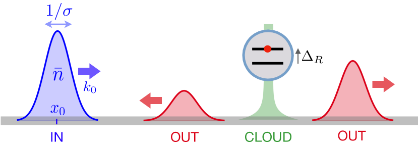
Figure 1: Illustration of the setup considered in this paper: a long transmission waveguide (grey horizontal line) is side-coupled to a two-level system, allowing the measurement of multi-photon scattering matrices in a typical two-terminal geometry from the reflection and transmission (outgoing states with arrows pointing outward) of a coherent state Gaussian wavepacket (incoming state with arrow pointing inward). A many-body polarization cloud lives in the central region (tied to the qubit) Snyman and Florens (2015). Frequency-conversion processes are extracted by a spectral and number state analysis of the outgoing wavepackets.

Our goal here is two-fold. First, we uncover new physical effects in non-linear many-body photon scattering by analyzing the photonic content of non-resonant emission spectra. One major observation is that significant non-linear emission arises from both RWA and non-RWA pathways. In light of standard knowledge in quantum optics, it comes as a surprise that non-RWA processes are found to dominate in magnitude the RWA non-linear response when off resonance. Indeed, in the regime of ultra-strong coupling, the linewidth of the qubit broadens substantially, leading to important non-resonant inelastic contributions to the scattering cross-section. Under a drive that is detuned in frequency above the resonance of the qubit, for instance, inelastic down-conversion occurs by the “splitting” of an incoming photon into several lower energy ones Goldstein et al. (2013). For larger power, there are similar processes involving an increasing number of incoming photons, all of which are described by counter-rotating terms. These processes are favored by a wide continuum of available outgoing multi-photon states. The surprising dominance of non-RWA processes can thus be interpreted as a consequence of the larger phase space of outgoing states for particle production.

Another dramatic many-body effect is uncovered by studying the correlations in time. We find that ultra-strong coupling leads to striking qualitative signatures in the photon statistics of a single emitter, namely incomplete anti-bunching on resonance at zero time-delay and strong bunching at finite delay, that are very prominent in the off-resonant case. These previously unrecognized features are quantitatively different from RWA results and constitute important signatures of particle production from an experimental point of view. A further indication of interesting many-body effects is that perturbative expansions for the elastic and inelastic emission spectra cannot be captured quantitatively.

Our second objective is to provide a general and powerful simulation toolbox to access the non-linear and inelastic processes involved to any order in the incoming beam power. This methodology relies on an expansion of the full many-body wavefunction (qubit+waveguide) in terms of multi-mode coherent states, using quantum superpositions of several classical-like configurations. It was introduced recently as a numerically controlled technique to capture the ground state Bera et al. (2014a, b) or quenched dynamics Gheeraert et al. (2017) in ultra-strong coupling wQED. Two original developments are made in the present manuscript. First, a new and more numerically efficient algorithm is proposed, which allows for the first time to tackle in a controlled way the many-body dynamics in waveguides composed of several thousands of modes. Second, we develop a many-body scattering protocol, that can be used to simulate realistic scattering setups, as shown in Fig. 1, allowing to deal with the challenging problem of many-body particle production in quantum optics. The resulting multi-photon emission processes in the output field are characterized precisely. Despite the coupling being weak to intermediate in magnitude, non-RWA contributions to these multi-photon processes open the door to a tremendously large Hilbert space. Typically our calculations manage up to five photons in the outgoing beam, which, for a long waveguide accounting for about 1000 environmental modes, leads to an effective Hilbert space of order $10^{15}\simeq 2^{50}$. It is quite remarkable that a quantum superposition of classical-like multi-mode coherent states can be harnessed as an efficient computing resource to address quantum many-body problems that are currently well beyond the reach of any brute force numerical method.

Regarding waveguides, several strategies are possible in order to bring these systems into a truly many-body territory, such as using the inductive coupling of a flux qubit to a low-impedance coplanar waveguide transmission line Forn-Díaz et al. (2017); Haeberlein et al. (2015), or tayloring a charge-like qubit with a capacitive coupling to a high impedance metamaterial Le Hur (2012); Goldstein et al. (2013); Snyman and Florens (2015). For this latter purpose, long chains of Josephson junctions Masluk et al. (2012); Bell et al. (2012); Altimiras et al. (2013); Weissl et al. (2015) constitute a promising platform that is currently under investigation Puertas Martínez et al. (2018) in the context of multi-mode ultra-strong coupling quantum optics. In any case, it remains challenging at present to control experimentally a strongly non-linear element constituting a true two-level system (such as the Cooper pair box or a flux qubit) that is also very well coupled to a designed environment, because non-linearity brings a high sensitivity to external noise sources. Designs based on a weakly non-linear qubit, such as a transmon Koch et al. (2007) ultra-strongly coupled to a waveguide Andersen and Blais (2017); Puertas Martínez et al. (2018) could offer an interesting alternative for high precision measurements, at the expense however of weakening the sought-after non-linear effects.

The paper is organized as follows. We first review in Sec. II the basic model of waveguide quantum electrodynamics, and develop a general many-body wavefunction approach for the study of inelastic photon emission by a single two-level system. Section III presents detailed inelastic emission spectra, in connection with the relevant physical processes. Section IV provides a comparison to standard results in quantum optics, based on the RWA, which can only account for processes in which two input photons are inelastically scattered, keeping the number of outgoing photons equal to two. This section closes with a discussion of the temporal correlations of the emitted light, showing several qualitative features of ultrastrong coupling. Finally, the perspectives section, Sec. V, discusses prospects for experimental measurements of these effects in superconducting circuits, and the need for developing further our theoretical tools in order to capture realistic aspects of Josephson waveguides beyond the spin-boson limit. Appendices contain technical derivations that should make the manuscript self-contained, and present details on the new algorithm proposed in this work.

II Many-body coherent state scattering formalism

II.1 Modeling a two-level system coupled to a waveguide

The main assumption that will be made in this study is the restriction of the atom to a perfect two-level system. This hypothesis is perfectly legitimate for strongly non-linear qubits, such as the Cooper pair box or the flux qubit Astafiev et al. (2010); Abdumalikov et al. (2010); Forn-Díaz et al. (2017); Magazzù et al. (2018), although these devices typically experience more strongly charge or flux noise compared to a transmon qubit (which is however weakly non-linear). Focusing on a two-level system aims to capture the maximum inelastic scattering cross-sections, due to its intrinsically high non-linearity. It is thus an excellent testbed to examine physics that is already quite rich, and to develop state-of-the-art methodologies in the most challenging situation from a computational point of view. Following this path, a qubit coupled to a full one-dimensional waveguide is quite generically expressed by the so-called spin-boson Hamiltonian (setting $\hbar$ to unity):

$$H=\frac{\Delta}{2}\sigma_{x}-\frac{\sigma_{z}}{2}\sum_{k\in\mathbb{R}}g_{k}^{\mathrm{full}}(a^{\phantom{e\dagger}}_{k}+a^{\dagger}_{k})+\sum_{k\in\mathbb{R}}\omega_{k}a^{\dagger}_{k}a^{\phantom{e\dagger}}_{k},$$ (1)

with $\Delta$ the bare splitting of the qubit levels. We stress that we do not work in the qubit eigenbasis here, but rather in a basis that makes the qubit-waveguide coupling diagonal, as described by the $\sigma_{z}$ term above (this corresponds for instance to the charge basis for a Cooper pair box that is capacitively coupled to a waveguide). This choice allows a natural description of the driving force behind the entanglement between the qubit and the waveguide, and sets the natural language for our numerical technique based on coherent states. The momentum dependence of the coupling constant $g_{k}^{\mathrm{full}}$ to mode $a^{\dagger}_{k}$ of the full waveguide depends on the device geometry and its physical parameters, such as inter-island capacitances, ground capacitances and inter-island Josephson energy. In the case where the waveguide is constructed from a Josephson junction array, Refs. Goldstein et al. (2013); Snyman and Florens (2015); Parra-Rodriguez et al. (2018) proposed explicit microscopic derivations of the coupling constants based on rather different designs. Similarly, the momentum dispersion of the eigenfrequencies $\omega_{k}$ of the photonic modes is determined by the microscopic details of the waveguide.

In what follows we will consider for simplicity a linear dispersion relation given by $\omega_{k}=|k|$ (taking the speed of light in the metamaterial $c=1$), and a simple parametrization of the coupling constant. For this purpose, and in order to simplify the problem, we start by folding the bosonic modes of the full waveguide onto a half-line, by defining even and odd modes:

$$a_{k}^{e}=\frac{1}{\sqrt{2}}\left(a_{k}+a_{-k}\right)\quad\textrm{and}\quad a_{k}^{o}=\frac{1}{\sqrt{2}}\left(a_{k}-a_{-k}\right),$$ (2)

so that the Hamiltonian (1) can be rewritten as

$$H=\frac{\Delta}{2}\sigma_{x}-\frac{\sigma_{z}}{2}\sum_{k>0}g_{k}(a^{e\phantom{\dagger}}_{k}+a^{e\dagger}_{k})+\sum_{k>0}\omega_{k}[a^{e\dagger}_{k}a^{e\phantom{\dagger}}_{k}\!+a^{o\dagger}_{k}a^{o\phantom{\dagger}}_{k}],$$ (3)

with the coupling constant to the even modes, $g_{k}=\sqrt{2}g_{k}^{\mathrm{full}}$. We choose a parametrization of the effective coupling constant $g_{k}$ given by the following spectral function:

$$J(\omega)=\sum_{k>0}\pi g_{k}^{2}\delta(\omega-\omega_{k})=2\pi\alpha\,\omega\,\mathrm{e}^{-\omega/\omega_{c}}.$$ (4)

This form of spectral function, although not completely generic, contains the main realistic ingredients of the qubit-waveguide interaction, such as a linear ohmic frequency dependence at low energy, and a rapid falloff near the plasma edge $\omega_{c}$, that we assume to be exponential in form. For a discretized momentum grid, we deduce that the coupling constant $g_{k}$ to even modes reads:

$$g_{k}=\sqrt{2\,\alpha\,\omega_{k}\,\delta k\,\mathrm{e}^{-\omega_{k}/\omega_{c}}},$$ (5)

where $\delta k$ is the wave-number spacing corresponding to the discretisation of the continuous momentum integral.

In the form of Hamiltonian (3), only the even modes are interacting with the qubit, while the odd modes are freely propagating. This allows us to write the state vector $\ket{\psi}$ as the direct product of the even sector $\ket{\psi^{e}}$ and the odd sector $\ket{\psi^{o}}$:

$$\ket{\psi}=\ket{\psi^{e}}_{e}\otimes\ket{\psi^{o}}_{o}=\ket{\psi^{e}}_{e}\ket{\psi^{o}}_{o}$$ (6)

provided the initial state can be decomposed accordingly. The dynamics in the odd sector is essentially trivial, while many-body effects have to be considered to capture the dynamics in the even sector, a topic that we address now.

II.2 Many-body quantum dynamics with multi-mode coherent states

The rationale behind the multi-mode coherent state (MCS) expansion is as follows. The only source of non-linearity in Hamiltonian (3) is the two-level system, and this non-linearity is transferred from a single degree of freedom (the qubit) to a large number of degrees of freedom (the modes of the waveguide). A first effect of this coupling is to dress the two qubit states by displacing the oscillators, as is clear from the $\sigma_{z}$ term in Eq. (3). This picture, which is only approximate when a single coherent state displacement is used, becomes quantitavely exact for the many-body ground state when superposing a small set of coherent states Bera et al. (2014b). Regarding the quantum dynamics, an input coherent state (as is relevant in our description of the scattering problem) remains stable only when turning the coupling to zero (classical-like propagation). At finite coupling, quantum fluctuations of the output field around the dominant classical trajectory are again accounted for by the superposition of additional Gaussian states. The strategy is thus to write the state vector in the even sector as a coherent state expansion, also referred to in the following as the multi-mode coherent state (MCS) ansatz Bera et al. (2014a, b); Snyman and Florens (2015):

$$|\Psi^{e}(t)\rangle=\sum_{m=1}^{N_{\mathrm{cs}}}\Big{[}p_{m}(t)|f_{m}(t)\rangle|\uparrow\rangle+q_{m}(t)|h_{m}(t)\rangle|\downarrow\rangle\Big{]},$$ (7)

where we have introduced the complex and time-dependent amplitudes $p_{m}(t)$ and $q_{m}(t)$ for each qubit component, with $m$ an index that labels the states used in the superposition. These multi-mode coherent states also occur as two discrete sets of states (one for each qubit component):

$$|f_{m}(t)\big{>}=\prod_{k=1}^{N_{\mathrm{modes}}}e^{[f_{k,m}(t)a^{e\dagger}_{k}-f_{k,m}^{*}(t)a^{e\phantom{\dagger}}_{k}]}|0\big{>}$$ (8)

and similar for $|h_{m}(t)\big{>}$. Due to the completeness of the coherent state basis on a discrete von-Neumann lattice Boon and Zak (1978), which naturally extends to the case of many modes, this discrete decomposition can target in principle an arbitrary state of the full Hilbert space for $N_{\mathrm{cs}}\to\infty$. However, for a fixed choice of Gaussian states, this leads to the unfathomable exponential cost that is typical of many-body quantum mechanics. The advantage of the MCS ansatz (7) lies in the variationally optimized time-dependent displacements $f_{k,m}(t)$, which allows one to track with high precision and low numerical cost the dynamics of the full state vector.

What is truly remarkable about such a multi-component multi-mode wavefunction is the relatively small number of coherent states $N_{\mathrm{cs}}$ that are necessary to capture both the static many-body ground state Bera et al. (2014b) and the complex dynamics resulting from quantum quenches Gheeraert et al. (2017), even deep in the ultra-strong coupling regime. The method works efficiently from the case of single mode cavities Bera et al. (2013); Cong et al. (2017); Leroux et al. (2018) up to the challenging situation of an infinite continuum Florens and Snyman (2015). As we will see later, addressing frequency conversion brings an additional difficulty in that non-linear emission signals are extremely faint when driving off resonance compared to the dominant elastic contributions, which requires very careful convergence of the numerics.

In principle, the exact Schrödinger dynamics, controlled by the Hamiltonian (3), can be derived from the real Lagrangian density:

$$\mathcal{L}=\big{<}\Psi(t)|\frac{i}{2}\overrightarrow{\partial_{t}}-\frac{i}{2}\overleftarrow{\partial_{t}}-\mathcal{H}|\Psi(t)\big{>},$$ (9)

by applying the time-dependent variational principle Kramer and Saraceno (1981), $\delta\int\mathrm{d}t\mathcal{L}=0$, upon arbitrary variations of the state vector (7) with respect to its set of variational parameters. This minimization obviously provides Euler-Lagrange equations

$$\frac{d}{dt}\frac{\partial\mathcal{L}}{\partial\dot{v}}=\frac{\partial\mathcal{L}}{\partial v}$$ (10)

for the set of variables $v=\{p_{m},q_{m},f_{k,m},h_{k,m}\}$, which can be solved by numerical integration Burghardt et al. (2003); Yao et al. (2013); Zhou et al. (2014); Bera et al. (2016); Gheeraert et al. (2017). The detailed form of the dynamical equations is provided in Appendix A.1. A new numerical algorithm, which supersedes the one proposed in Ref. Gheeraert et al. (2017) and allows to deal with up to thousands of modes, is presented in Appendix A.2.

II.3 General coherent state scattering formalism

Now that we have obtained exact dynamical equations for the time evolution under the spin-boson Hamiltonian (1), we need to prepare our initial state in order to perform scattering simulations according to the scheme in Fig. 1. The generic difficulty is that the qubit is dressed non-perturbatively by a cloud of photons Leggett et al. (1987); Peropadre et al. (2013); Bera et al. (2014b); Sanchez-Burillo et al. (2014); Snyman and Florens (2015); Díaz-Camacho et al. (2016) in the ultra-strong coupling regime, so that this ground state assumes a many-body character. Thanks to the MCS ansatz introduced in eq. (7), we can efficiently express the static ground state of the joint qubit and waveguide system in terms of multi-mode coherent states:

$$|\Psi^{\mathrm{GS}}\rangle=\sum_{m=1}^{N^{\mathrm{GS}}_{\textrm{cs}}}p^{\mathrm{GS}}_{m}\Big{[}|f^{\mathrm{GS}}_{m}\rangle_{e}|\uparrow\rangle-|-f^{\mathrm{GS}}_{m}\rangle_{e}|\downarrow\rangle\Big{]}|0\rangle_{o},$$ (11)

where we enforced the $\mathbb{Z}_{2}$ spin-symmetry of the spin-boson Hamiltonian (3) to simplify the expression. We have also used the fact that the odd modes do not interact with the qubit, so that the ground state displacements include only even modes in Eq. (11), and the odd modes are placed in the vacuum state.

By implementing numerically a variational optimization Bera et al. (2014b, a), one can determine the set of weights $p^{\mathrm{GS}}_{m}$ and displacements $f^{\mathrm{GS}}_{k,m}$, and thus obtain a nearly exact result for the ground state up to negligible numerical error. Conveniently, only a small number of coherent states $N^{\mathrm{GS}}_{\textrm{cs}}$, typically less than 10, are required in the realistic domain of parameters of the spin-boson model.

The second step in the scattering picture of Fig. 1 is to include a wavepacket (with arrow pointing inward) impinging on the dressed ground state. We will work in what follows with a single coherent state pulse as input, which is realistic in terms of the classical sources used in actual experiments. Let us denote $z_{k}$ the displacement of the incoming wave-packet in mode $k$ of the physical waveguide, and $z_{x}$ its Fourier transform to real space:

$$z_{x}=\int_{-\infty}^{\infty}\frac{dk}{\sqrt{2\pi}}e^{+ikx}z_{k}.$$ (12)

We choose to use here a Gaussian-shaped wavepacket

$$z_{k}=\sqrt{\bar{n}}\left(\frac{1}{2\pi\sigma^{2}}\right)^{\frac{1}{4}}e^{-\frac{(k-k_{0})^{2}}{4\sigma^{2}}}e^{-i(k-k_{0})x_{0}}e^{-ik_{0}x_{0}/2},$$ (13)

corresponding to a signal initially centered around position $x_{0}$ in the waveguide, with mean wavenumber $k_{0}$, spatial extent $1/\sigma$, and total intensity corresponding to $\bar{n}$ photons on average, as illustrated on Fig. 1. The associated real space wavepacket is then

$$z_{x}=\sqrt{\bar{n}}\left(\frac{2\sigma^{2}}{\pi}\right)^{\frac{1}{4}}e^{-(x-x_{0})^{2}\sigma^{2}}e^{+ik_{0}(x-x_{0})}e^{+ik_{0}x_{0}/2}.$$ (14)

Note that these amplitudes are both normalized so that $\int_{-\infty}^{\infty}dx|z_{x}|^{2}=\int_{-\infty}^{\infty}dk|z_{k}|^{2}=\bar{n}$.

The even and odd parts of the incoming wavepacket are then defined strictly for $k>0$ as

$$z_{k}^{e}=\frac{1}{\sqrt{2}}\left(z_{k}+z_{-k}\right)\quad\textrm{and}\quad z_{k}^{o}=\frac{1}{\sqrt{2}}\left(z_{k}-z_{-k}\right).$$ (15)

Since even and odd modes commute, we can then define a displacement operator $D(z)$ for the initial incoming wave-packet which verifies:

$$\ket{z^{e},z^{o}} =D(z)\ket{0}=D(z^{e})D(z^{o})\ket{0}$$ (16)

$$=e^{\sum_{k>0}\left(z_{k}^{e}a_{k}^{e\dagger}-z_{k}^{e*}a_{k}^{e}\right)}e^{\sum_{k>0}\left(z_{k}^{o}a_{k}^{o\dagger}-z_{k}^{o*}a_{k}^{o}\right)}\ket{0}.$$

The final step in the initialization of the state vector is to combine the incoming wavepacket coherent state $z_{k}$ with the displacements entering the full many-body ground state (11). Straightforward calculations, shown in Appendix A.3, lead to the following explicit expression for the input state:

$$\ket{\Psi^{\mathrm{IN}}} = \sum_{m=1}^{N^{\mathrm{GS}}_{\textrm{cs}}}p^{\mathrm{GS}}_{m}\Big{[}\ket{\uparrow}e^{\frac{1}{2}\sum_{k>0}\left(z_{k}^{e}f_{k,m}^{\mathrm{GS}*}-z_{k}^{e*}f_{k,m}^{\mathrm{GS}}\right)}e^{\sum_{k>0}\left[\left(f_{k,m}^{\mathrm{GS}}+z_{k}^{e}\right)a_{k}^{e\dagger}-\left(f_{k,m}^{\mathrm{GS}}+z_{k}^{e}\right)^{*}a_{k}^{e}\right]}$$ (17)

$$-\ket{\downarrow}e^{\frac{1}{2}\sum_{k>0}\left(-z_{k}^{e}f_{k,m}^{\mathrm{GS}*}+z_{k}^{e*}f_{k,m}^{\mathrm{GS}}\right)}e^{\sum_{k>0}\left[\left(-f_{k,m}^{\mathrm{GS}}+z_{k}^{e}\right)a_{k}^{e\dagger}-\left(-f_{k,m}^{\mathrm{GS}}+z_{k}^{e}\right)^{*}a_{k}^{e}\right]}\Big{]}\ket{0}_{e}\ket{z^{o}}_{o}.$$

The many-body scattering theory thus amounts to use state (17) as the initial condition for the dynamical equations of motion (10) performed in the even sector, see Eqs. (28)-(29) for their full explicit form. During the dynamics, as the incoming wavepacket impinges on the qubit, the necessary number of coherent states $N_{\mathrm{cs}}$ will sensibly grow from the initial value $N_{\mathrm{cs}}^{\mathrm{GS}}$ due to non-classical emission, therefore requiring to add extra coherent states to the state vector when needed (the procedure is detailed in Appendix A.5). In the odd sector, which is completely decoupled from the qubit, the related displacements are trivially evolving in time according to $i\dot{z}_{k}^{o}=\omega_{k}z_{k}^{o}$, and a single coherent state is enough for the whole time-evolution.

After a given time $T$ long enough to ensure interaction of the wavepacket with the qubit and subsequent decoupling of the two outgoing wavepackets from the many-body cloud surrounding the qubit (in the reflection and transmission channel of the full 1D waveguide), one expects on general grounds (since the spin-boson model is non-integrable with a realistic dispersion) a factorization of the final wavefunction as:

$$\ket{\Psi(T)}=\ket{\Psi^{\mathrm{GS}}}\otimes\ket{\Psi^{\mathrm{OUT}}},$$ (18)

where $\ket{\Psi^{\mathrm{GS}}}$ is the many-body ground state of the spin-boson model and $\ket{\Psi^{\mathrm{OUT}}}$ a many-body outgoing wavepacket that contains a non-trivial decomposition of the emitted signal in terms of a large number of multi-mode coherent states (typically $N_{cs}^{\rm OUT}\sim 20-30$):

$$\ket{\Psi^{\mathrm{OUT}}}=\sum_{m=1}^{{N^{\mathrm{OUT}}_{\textrm{cs}}}}p^{\mathrm{OUT}}_{m}\prod_{k=1}^{N_{\mathrm{modes}}}e^{[f_{k,m}^{\mathrm{OUT}}a^{e\dagger}_{k}-f_{k,m}^{\mathrm{OUT*}}a^{e\phantom{\dagger}}_{k}]}|0\big{>}.$$ (19)

The extraction procedure for the outgoing weights $p^{\mathrm{OUT}}_{m}$ and displacements $f_{k,m}^{\mathrm{OUT}}$ is given in Appendix A.3. The factorization property (18) occurs because the spin-boson model (with a macroscopic number of modes) is a truly dissipative system, always showing a path for relaxation. In practice, this hypothesis can be checked from the numerical calculations by observing that the dressed qubit does not show correlations with the outgoing photons. Indeed, any observable of the qubit relaxes back to its initial equilibrium value at the end of the scattering protocol. Also, the nature of the scattered photons does not depend on how one traces out the qubit density matrix. We now proceed to the analysis of the transmission and spectral properties of this scattered many-body wave-packet.

III Multiphoton inelastic scattering

III.1 Elastic emission and high power saturation

As a first illustration for our dynamical many-body scattering method, we investigate the elastic reflection as a function of the frequency and power of the incoming signal. This problem is particularly challenging because of the combination of non-perturbative ultra-strong coupling with non-equilibrium effects that arise at finite input power. Ultra-strong coupling scattering at non-vanishing power has been addressed previously with approximate techniques Le Hur (2012); Bera et al. (2016); Shi et al. (2018a); Magazzù et al. (2018) and with more advanced numerical methods Peropadre et al. (2013); Sanchez-Burillo et al. (2014). However, systematic extraction of many-body scattering matrices has not been performed to our knowledge.

Our calculation scheme proceeds similarly to an experimental setup: the incoming Gaussian coherent-state wavepacket, shown schematically as the incoming distribution of photons in real space in Fig. 1, is initialized to the left of the qubit. The qubit is placed at position $x=0$ as seen from its sharply decreasing photonic cloud Snyman and Florens (2015) which is present in both the input and output ports, but remains statically bound to the central impurity. After propagation towards the qubit and subsequent interaction, the photon flux decouples at long times, and is separated into a reflected left going ($k<0$) signal and a transmitted right going ($k>0$) signal, both shown with arrows pointing outward in Fig. 1. Note that in all the simulations made in this paper, we have considered the linewidth $\sigma$ of the wavepacket in $k$-space to be smaller than the qubit linewidth $\Gamma$ (in order to achieve high spectroscopic resolution), but large enough to keep the simulations on a reasonable system size (typically we consider from $N_{\mathrm{modes}}=1000$ to $N_{\mathrm{modes}}=3000$ modes for the chain used in the even sector). All calculations are done in the units of the plasma frequency $\omega_{c}$ as defined in the spectral density (4), and the wavepacket linewidth appearing in Eq. (13) is taken as $\sigma=0.005\omega_{c}$, unless indicated otherwise.

We define the reflection and transmission coefficients in the following way:

$$T=\frac{\sum_{k>0}\braket{a^{\dagger}_{k}a^{\phantom{e\dagger}}_{k}}_{\mathrm{out}}}{\sum_{k>0}\braket{a^{\dagger}_{k}a^{\phantom{e\dagger}}_{k}}_{\mathrm{in}}}\quad\textrm{and}\quad R=\frac{\sum_{k<0}\braket{a^{\dagger}_{k}a^{\phantom{e\dagger}}_{k}}_{\mathrm{out}}}{\sum_{k>0}\braket{a^{\dagger}_{k}a^{\phantom{e\dagger}}_{k}}_{\mathrm{in}}},$$ (20)

where we have denoted $\braket{\ldots}_{\mathrm{in}}$ the average over the state vector corresponding to the coherent incoming wave-packet before scattering, and $\braket{\ldots}_{\mathrm{out}}$ the average over the many-body outgoing wave-packet after scattering. Both are obtained from the full state vector (19) by simply filtering out in real-space the polarization cloud associated with the ground state, as explained in Appendix A.3.

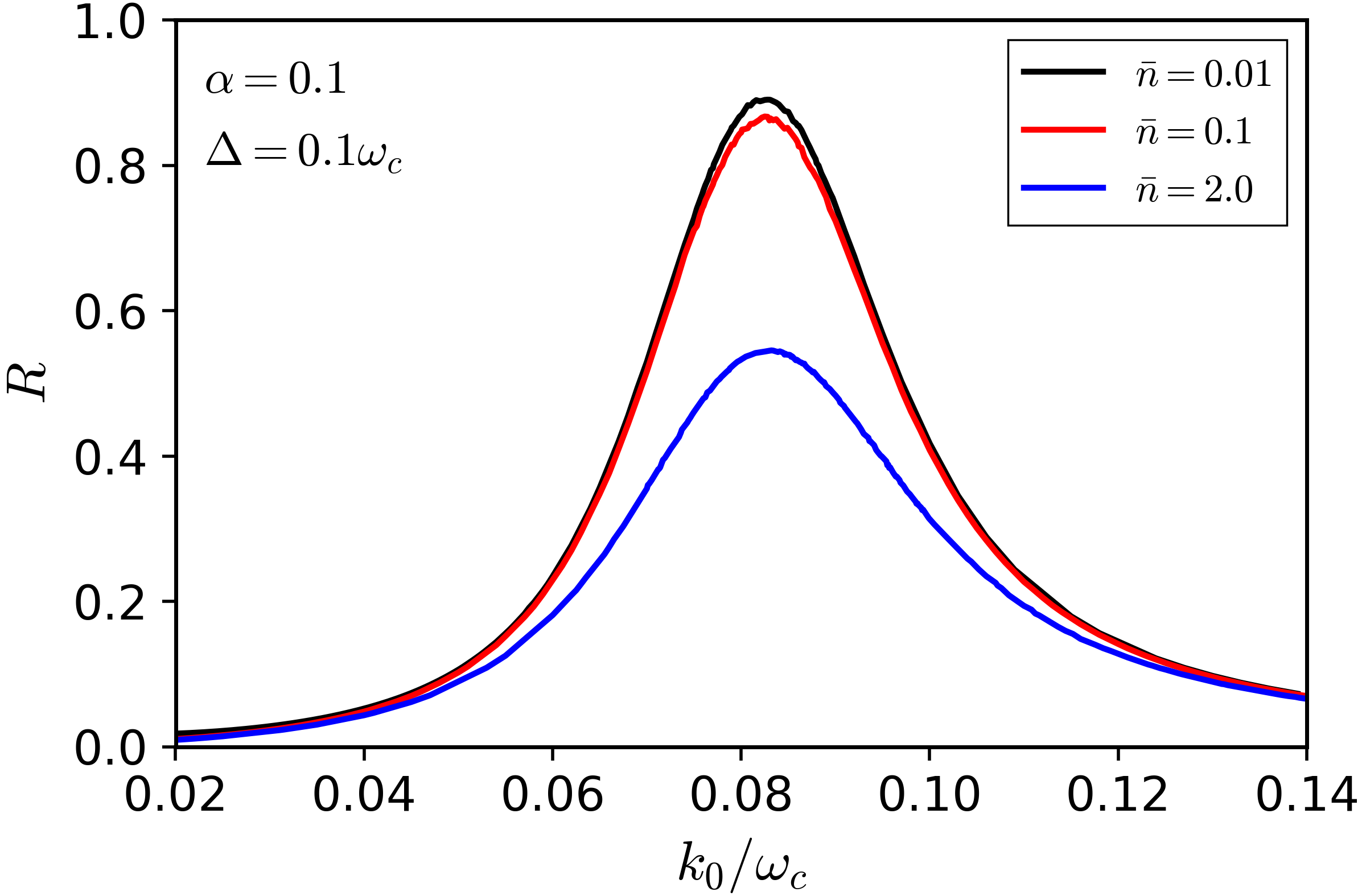
Figure 2: Saturation effects in the reflection coefficient Eq. (20) as a function of incoming wavevector $k_{0}$, for three different amplitudes $\bar{n}=0.01,0.1,2.0$ of the input, with a wavepacket width $\sigma=0.005\omega_{c}$. These curves correspond to converged numerical data with up to $N_{\mathrm{cs}}=16$ coherent states in the MCS wavefunction (7). The bare qubit frequency is $\Delta=0.1\omega_{c}$ and the dimensionless light-matter interaction is $\alpha=0.1$, leading to a sizeable renormalized qubit frequency $\Delta_{R}\simeq 0.08\omega_{c}$.

Results for different values of the incoming power are shown in Fig. 2. The probability of reflection generally increases on resonance; indeed, for elastically scattered photons, interference effects cause almost complete reflection when exactly on resonance. For small values of the incoming power ($\bar{n}=0.01$ and $\bar{n}=0.1$), for which the initial coherent state wavepacket has a very small probability of containing Fock states with more than 1 photon, one can note that the reflection only reaches $R\simeq 0.9$ at peak value. This incomplete reflection of the photons arises from the finite linewidth of the incoming wavepacket, and not from inelastic losses. Since our incoming Gaussian pulse is not perfectly monochromatic, the modes at the edge of a resonant incoming beam (centered at $k_{0}=\Delta_{R}$) are slightly off-resonant and do not get fully reflected by the qubit. Even in the present case of a relatively small light matter coupling $\alpha=0.1$, many-body effects due to the ultra-strong coupling are apparent in the reflection curve of Fig. 2. First, a non-Lorentzian asymmetric lineshape is obtained, with a high energy tail more prominent than at low energy. In addition, we clearly observe a substantial renormalization of the qubit frequency $\Delta_{R}\simeq 0.08\omega_{c}$ from its bare value $\Delta=0.1\omega_{c}$.

For higher incoming power, one physically expects saturation effects to take place, and these are clearly evidenced by the curve with average number of photons $\bar{n}=2.0$ in Fig. 2. We stress that converging such computations in the high power regime is quite challenging, and approximate techniques such as a single coherent state truncation lead to uncontrollable noise levels, as found in previous work Bera et al. (2016). We show in detail in Appendix A.4 that the reflection curve converges smoothly at $\bar{n}=2.0$ for about $N_{\mathrm{cs}}=16$ coherent states in the MCS state vector (7). This is also confirmed by a systematic control of the error, as done previously for quantum quench protocols Gheeraert et al. (2017).

III.2 Off-resonant frequency-conversion spectra

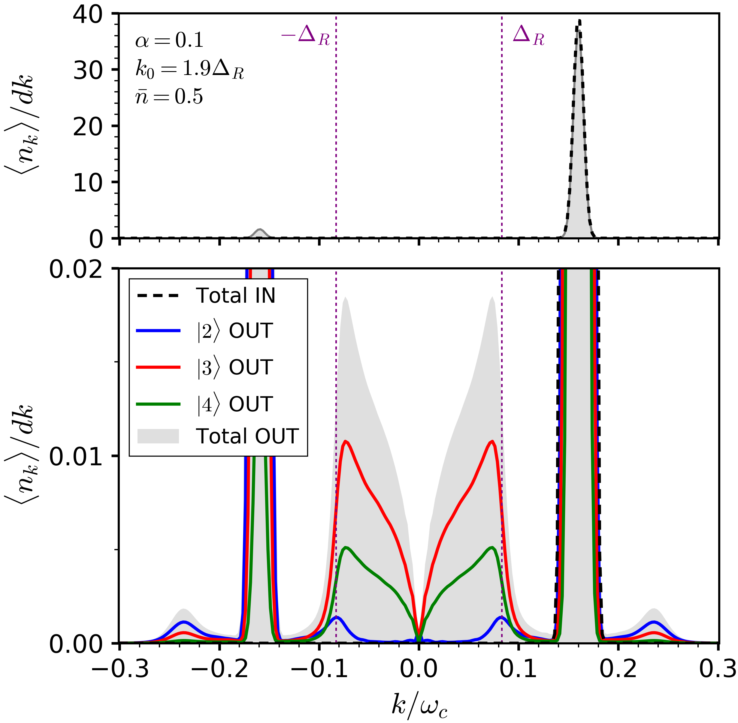
Figure 3: Mean density of photons at momentum $k$ in the outgoing wave-packet (the incoming wavepacket is displayed as a dashed line); bottom panel is a zoom of top. The total outgoing signal (gray shaded) is decomposed into Fock resolved excitations (in full lines) with $N=2$ (bottom curve), $N=3$ (top curve) and $N=4$ (middle curve) photons, in order to highlight the processes of Fig. 4. The parameters for this simulation are the incoming wave-packet wave-number $k_{0}=0.16\omega_{c}$ and linewidth $\sigma=0.005\omega_{c}$, the mean photon number $\bar{n}=0.5$, the qubit bare energy $\Delta=0.1\omega_{c}$, and the coupling strength $\alpha=0.1$. Simulations were performed by considering a wavefunction containing $N_{\mathrm{cs}}=30$ coherent states, and $N_{\mathrm{modes}}=1200$ modes.

We now turn to analyzing the emitted radiation in the off-resonant case, in which the system is excited at a frequency $k_{0}$ above the renormalized qubit transition frequency $\Delta_{R}$. A typical inelastic spectrum is shown in Fig. 3, here for $k_{0}=0.16\omega_{c}$, $\Delta_{R}=0.08\omega_{c}$, and an injected $\bar{n}$ of $0.5$. The stronger transmission relative to reflection (upper panel) simply reflects the off-resonant situation $k_{0}\approx 2\Delta_{R}$, in agreement with the reflection curve in Fig. 2. The vertical scale is expanded in the lower panel, so that the inelastic contributions are made apparent at the foot of the large reflection and transmission elastic peaks located at $\pm k_{0}$. Note that the actual linewidth of this elastic peak, set by $\sigma=0.005\omega_{c}$, is in fact much smaller than what the lower panel seems to indicate, because the maximum peak amplitude is 2000 times higher that the scale of the graph. The gray-shaded curve displays the expectation value of the total number of outgoing photons $\braket{a^{\dagger}_{k}a^{\phantom{e\dagger}}_{k}}_{\rm{out}}$ while the dashed line indicates the total number of incoming photons $\braket{a^{\dagger}_{k}a^{\phantom{e\dagger}}_{k}}_{\rm{in}}$ centered around $k_{0}$. The first striking result is the broad spectrum of emission extending from the qubit frequency $\Delta_{R}$ all the way down to $k=0$.

The full lines display how the total outgoing photon contribution is distributed among different Fock states $\ket{N}$ with photon number $N=2,3,4$, allowing us to assess the nature of particle production. Our method to obtain these photon-number resolved amplitudes by considering the probability of all the possible single- and multi-photon states for a given momentum $k$ is explained in Appendix A.6. Note that the majority of the inelastic emission involves 3 and 4 photon contributions. Since the incoming average photon number is only $0.5$, clearly substantial particle production is occurring! Both the broad inelastic spectrum and particle production are quintessentially ultra-strong coupling phenomenona.

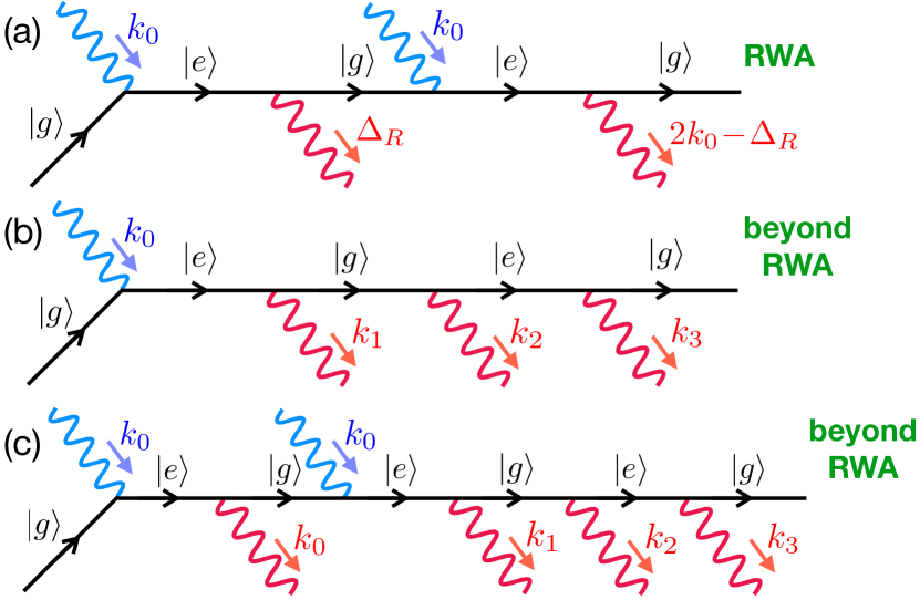
Figure 4: Diagrammatic representation of some non-linear photon processes occurring during scattering onto a two-level system. Panel (a) is a RWA frequency exchange process restricted at the two photon level, which shows two sharp emission lines at $\Delta_{R}$ and $2k_{0}-\Delta_{R}$ (due to energy conservation). Panel (b) shows the non-RWA one photon to three photon conversion Goldstein et al. (2013), which leads to a broad emission continuum, sharply peaked at the resonance $\Delta_{R}$ in the case of an off-resonant drive. Panel (c) is a similar particle producing process, now with two input photons, one being down converted to three photons, the other photon being elastically scattered.

For an initial understanding of the various contributions to this spectrum, we consider a schematic diagrammatic perturbation theory as shown in Fig. 4. For two incoming photons, an inelastic RWA process can occur by distributing the total incoming energy $2k_{0}$ into a resonant photon at $\Delta_{R}$ and another at $2k_{0}-\Delta_{R}$ as shown in panel (a). However, for a single incoming photon with momentum $k_{0}$, since the emission is still maximum at the (renormalized) resonant qubit frequency $\Delta_{R}$, an excess energy of $k_{0}-\Delta_{R}$ must be distributed between two extra outgoing photons (in order to properly relax to the ground state). The accessible non-resonant states thus lead to the non-RWA 3-photon emission process shown in panel (b). In general, the two extra photons that are produced are not resonant, and the amplitude of the total process is sizable only because of the ultra-strong coupling regime. Indeed, the elastic reflection curve of Fig. 2 is spectrally very broad, and emission does not necessarily occur strictly on resonance.

The non-RWA nature of the particle production process is obvious from the non-conservation of excitations: the middle outgoing arrow in Fig. 4(b) corresponds to the emission of a photon upon excitation of the two-level system (instead of the usual de-excitation). Four photon production is also displayed in panel (c) for an input state with two photons. In this case, one input photon is elastically scattered at $k_{0}$, while the second input photon splits into three photons similar to the process in panel (b). Since the RWA $2\to 2$ process in panel (a) and the non-RWA $2\to 4$ process in panel (c) come at the same order in the input power, they can be used to directly compare the relative strength of RWA and non-RWA processes. All three processes of Fig. 4 are clearly observed in the spectrum shown in Fig. 3, as the emission amplitude is decomposed into photon number states $N=2,3,4$. In view of the wide use of the RWA in the quantum optics context, the main surprise in these results (to be discussed in more detail below) is that non-RWA processes strongly dominate in amplitude the RWA processes.

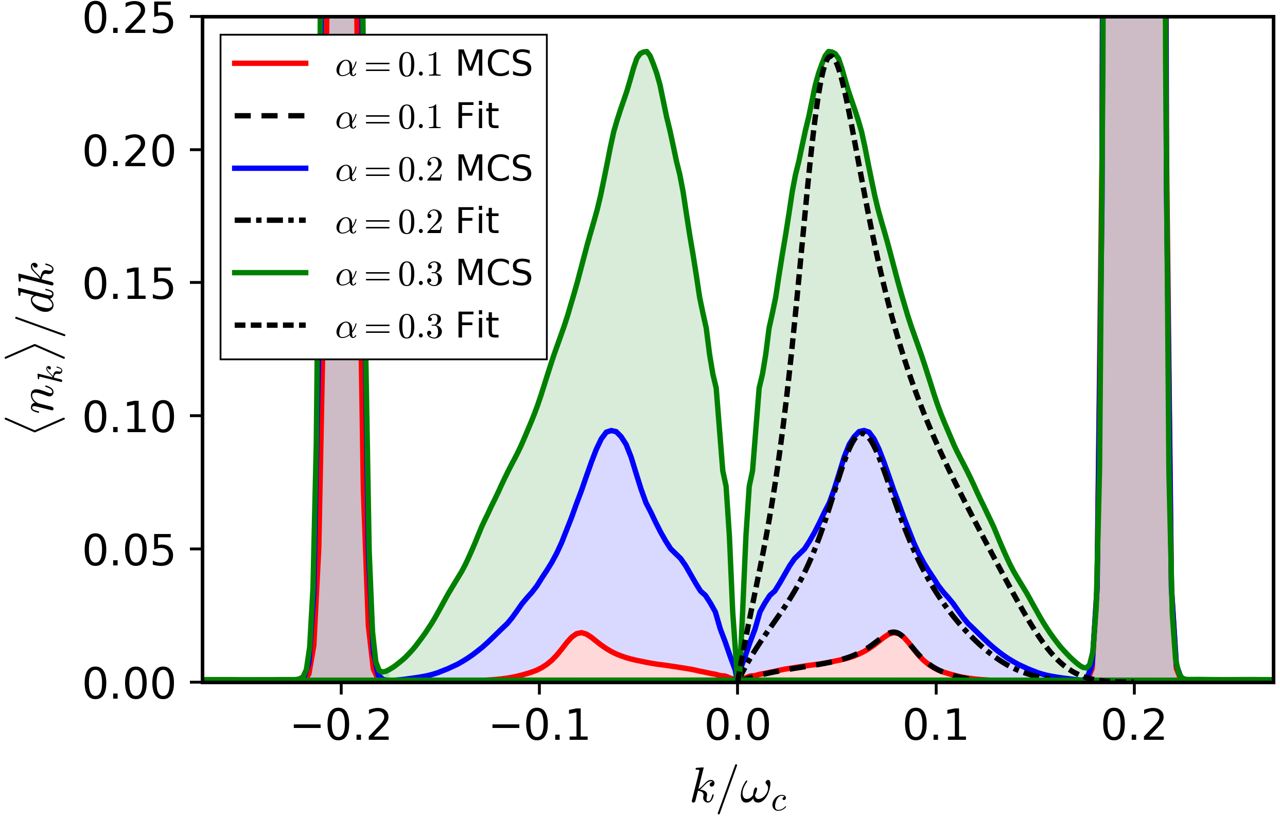
Figure 5: Frequency conversion spectrum by going deeper in the ultra-strong coupling regime ($\alpha=0.1,0.2,0.3$, bottom to top curves) for an off-resonant incoming wavevector $k_{0}=0.2\omega_{c}$. Parameters are otherwise taken as in Fig. 3. Although the resonance frequency $\Delta_{R}$ and inelastic linewidth $\gamma_{R}^{\mathrm{inel}}$ were fitted, one observes increasing deviations to the fitting formula (B.1) at larger $\alpha$. Enhanced scattering of low-energy modes, precursor of the Kondo regime, originate from non-perturbative many-body corrections beyond the lowest order perturbation theory of Ref. Goldstein et al. (2013).

Some of the off-resonant processes were previously predicted perturbatively by Goldstein et al. Goldstein et al. (2013) in the $\alpha\to 0$ limit and at the Toulouse limit, and we are able to characterize quantitatively the non-linear emission for the first time at finite $\alpha$ values, as seen in Fig. 5. The main effect brought by stronger coupling is a further renormalization of the spontaneous emission line $\Delta_{R}$ down to lower values, as well as a global increase of the probability for inelastic conversion. Interestingly, we find that the perturbative formula (B.1) cannot quantitatively describe our data anymore in this regime, even when allowing to fit the inelastic linewidth. Perturbation theory thus fails to capture the pile-up of low-energy photons found in the numerical simulations, which signals the approach to the incoherent Kondo regime, in which the qubit resonance is fully washed out. A detailed study of non-linear spectra as a function of incoming momentum is given in Appendix B.1.

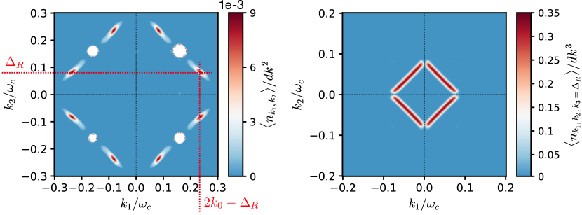
Figure 6: Left panel: probability distribution of the two-photon states $|\alpha_{k_{1},k_{2}}|^{2}/dk^{2}$ corresponding to the 2-photon curve in Fig. 3. The clear inelastic sidebands correspond to frequency exchange between 2 photons. Right panel: probability density distribution $|\alpha_{k_{1},k_{2},k_{3}=\Delta_{R}}|^{2}/dk^{3}$ of the three-photon states in which one photon is at the resonance frequency $k_{3}\approx\Delta_{R}$, corresponding to the 3-photon curve in Fig. 3. The emission continuum associated to particle production is revealed by the diamond-shaped line.

III.3 Particle production processes

We now investigate more precisely the photonic content of the emitted radiation in the inelastic channel. Let us start with the 2-photon particle-conserving RWA contribution (bottom full line $N=2$ in Fig. 3) forming two lobes symmetrically arranged around the main elastic peak (at $k_{0}=0.16\omega_{c}$). The lowest energy lobe is centered around $k\simeq 0.08\omega_{c}\simeq\Delta_{R}$ corresponding to the spontaneous reemission of the qubit, while the high energy lobe is located around $k\simeq 0.24\omega_{c}\simeq 2k_{0}-\Delta_{R}$, as expected from energy conservation [panel (a) in Fig. 4]. A closer view into this two-photon joint emission process is given by the complete two-photon probability distribution $|\alpha_{k_{1}\,k_{2}}|^{2}$ that is plotted in the top panel of Fig. 6 (see Appendix A.6 for details). The main 2-photon elastic peaks are the white disks located at $[\pm k_{0},\pm k_{0}]$, that have been cut off in order to magnify the small inelastic contributions. From the lateral inelastic peaks, one can immediately read-off the two-photon frequency conversion process in which two photons with energy $k_{0}$ redistribute their energy into one photon with momentum $\Delta_{R}$ and another with energy $2k_{0}-\Delta_{R}$.

The inelastic spectrum originating from the conversion of a single incoming photon into three outgoing photons, with probability $\braket{n_{k}}_{\mathrm{3photon}}$ of measuring one of these photons at energy $k$, is represented by the middle full line in Fig. 3. This inelastic lineshape presents quite unusual features: a sharp resonance at the qubit frequency $\Delta_{R}$, a broad continuum extending from zero energy up to the foot of the elastic peak, and a small lobe at the same energy $2k_{0}-\Delta_{R}$ as the previous two-photon conversion process. The latter is easily understood as an input of three photons with momentum $k_{0}$, out of which one photon is elastically scattered, while the other two are RWA frequency converted to $\Delta_{R}$ and $2k_{0}-\Delta_{R}$ (similar to the previous $2\to 2$ RWA process). We have checked that this $3\to 3$ RWA process becomes relatively weaker in amplitude as the input power $\bar{n}$ is turned down, and is indeed associated to a three-photon input.

The broad low-energy continuum is readily explained by the 1-photon to 3-photon non-RWA conversion process shown in panel (b) of Fig. 4. This interpretation is backed up by studying in the right panel of Fig. 6 the probability distribution $|\alpha_{k_{1}k_{2}k_{3}=\Delta_{R}}|^{2}$ of 3-photon outgoing states for which one of the three outgoing modes is resonant, $k_{3}=\Delta_{R}$. To understand this diamond-shaped pattern, one can observe that the process leading to the diagonal line in the top-left quadrant can easily be parametrized as:

$$\ket{k_{0}}\rightarrow\ket{\Delta_{R}}\ket{\Omega}\ket{k_{0}-\Delta_{R}-\Omega}\;\mathrm{with}\;\Omega\in[0:k_{0}-\Delta_{R}].$$

which basically expresses the conservation of energy between the input and the output. Note that in the on-resonant situation (or for a drive at frequency below $\Delta_{R}$), all emitted photons present energies below the qubit frequency.

The next section investigates how the complete inelastic emission spectra compare with the standard RWA prediction in quantum optics. This comparison will provide not only a benchmark of our simulations, but also several physical signatures that cannot be captured without the inclusion of particle production processes.

IV Success and failure of the RWA for non-linear emission

IV.1 RWA inelastic conversion

To highlight particle production that arises at ultra-strong coupling, we now compare our MCS simulations to a direct treatment within the RWA, an approximation which conserves the number of excitations. Transport under the RWA is obtained in the framework of input-output theory. Within the RWA, it is convenient to work in the basis that diagonalizes the qubit. After applying the rotating wave approximation to the Hamiltonian (1) and assuming a frequency-independent coupling constant $g_{k}=\sqrt{\alpha\Delta_{R}}$, one finds that the system is described by the Hamiltonian

$$H = \frac{1}{2}\Delta\sigma^{z}+\int d\omega\,\,\frac{g}{2}\big{[}\sigma^{+}(r_{\omega}+l_{\omega})+h.c.\big{]}$$

$$+\int d\omega\,\,\omega\big{(}r_{\omega}^{\dagger}r_{\omega}-l_{\omega}^{\dagger}l_{\omega}\big{)},$$

where $\sigma^{+}$ is the raising operator of the qubit and $r_{\omega}(l_{\omega})$ is the annihilation operator for the right(left)-going mode of frequency $\omega$. We adapt standard input-output theory for a monochromatic input Walls and Milburn (2007); Fan et al. (2010); Kocabaş et al. (2012); Lalumière et al. (2013) to our case of an incoming wavepacket with finite energy resolution. The input-output relation remains the usual one, $r_{\text{out}}(t)=r_{\text{in}}(t)-i\sqrt{\pi/2}\,g\,\sigma^{-}(t)$ and similarly for the left-going field $l_{\text{in/out}}$. This allows one to find the properties of the outgoing field from a master equation for the qubit. In this way the power spectrum is calculated through the first-order correlation function $G^{(1)}(t_{1},t_{2})=\braket{a_{\text{out}}^{\dagger}(t_{1})a_{\text{out}}(t_{2})}$ by a Fourier transform

$$S[\omega]=\frac{1}{2\pi}\int_{0}^{T}dt_{1}\int_{0}^{T}dt_{2}\,G^{(1)}(t_{1},t_{2})e^{i\omega(t_{2}-t_{1})}.$$ (22)

We assume that the qubit is located at $x=0$ while the input and output ends are located at $x=-T/2$ and $T/2$ respectively ($c=1$). From the definition (13), we can write the wavepacket in frequency as

$$z(\omega)=\sqrt{\bar{n}}\left(\frac{1}{2\pi\sigma^{2}}\right)^{\frac{1}{4}}e^{-\frac{(\omega-k_{0})^{2}}{4\sigma^{2}}}e^{i(\omega-k_{0})T/2},$$ (23)

through which the input coherent state is defined as $\ket{z^{+}}=\exp{\big{[}\int dk\,z(\omega)\,r_{\text{in}}^{\dagger}(\omega)-h.c.\big{]}}\ket{0}$, where $r_{\text{in}}^{\dagger}(\omega)$ is the standard monochromatic input operator Walls and Milburn (2007); Fan et al. (2010); Kocabaş et al. (2012); Lalumière et al. (2013) of input-output theory. The input operator describing our wavepacket then satisfies

$$r_{\text{in}}(t)\ket{z^{+}}=\frac{1}{\sqrt{2\pi}}A(t)e^{-ik_{0}t}\ket{z^{+}}\text{ and }l_{\text{in}}(t)\ket{z^{+}}=0,$$ (24)

where $A(t)=\tilde{A}e^{-\sigma^{2}(t-T/2)^{2}}$ with $\tilde{A}=\sqrt{2\bar{n}\sigma}(2\pi)^{1/4}$ is the change of driving amplitude on the qubit with time as the Gaussian wavepacket passes by.

A master equation for the qubit density matrix $\rho_{s}$ is then obtained by transforming to the Schrödinger picture,

$$\begin{split}\frac{\partial}{\partial t}\rho_{\text{s}}=&-i\big{[}\frac{\delta}{2}\sigma^{z}+gA(t)\sigma_{+}+h.c.\,,\rho_{\text{s}}\big{]}\\ &+\pi g^{2}\big{(}\sigma_{-}\rho_{\text{s}}\sigma_{+}-\frac{1}{2}\{\rho_{\text{s}},\sigma_{+}\sigma_{-}\}\big{)},\end{split}$$ (25)

where a rotating frame given by $k_{0}\sigma^{z}/2$ has been used. Note that decay rate is $\Gamma=\pi g^{2}=\pi\alpha\Delta_{\text{R}}$. For the reflected light, the power spectrum can be shown to be

$$S_{\text{L}}[\omega]=g^{2}\int_{0}^{T}dt\int_{-t}^{T-t}d\tau\braket{\sigma_{+}(t)\sigma_{-}(t+\tau)}e^{i(\omega-k_{0})\tau};$$ (26)

two additional interference terms appear in the power spectrum for the transmitted light and are not given here. The desired correlation function $\braket{\sigma_{+}(t)\sigma_{-}(t+\tau)}$ can be calculated through the master equation (25) and the quantum regression theorem Carmichael (1993).

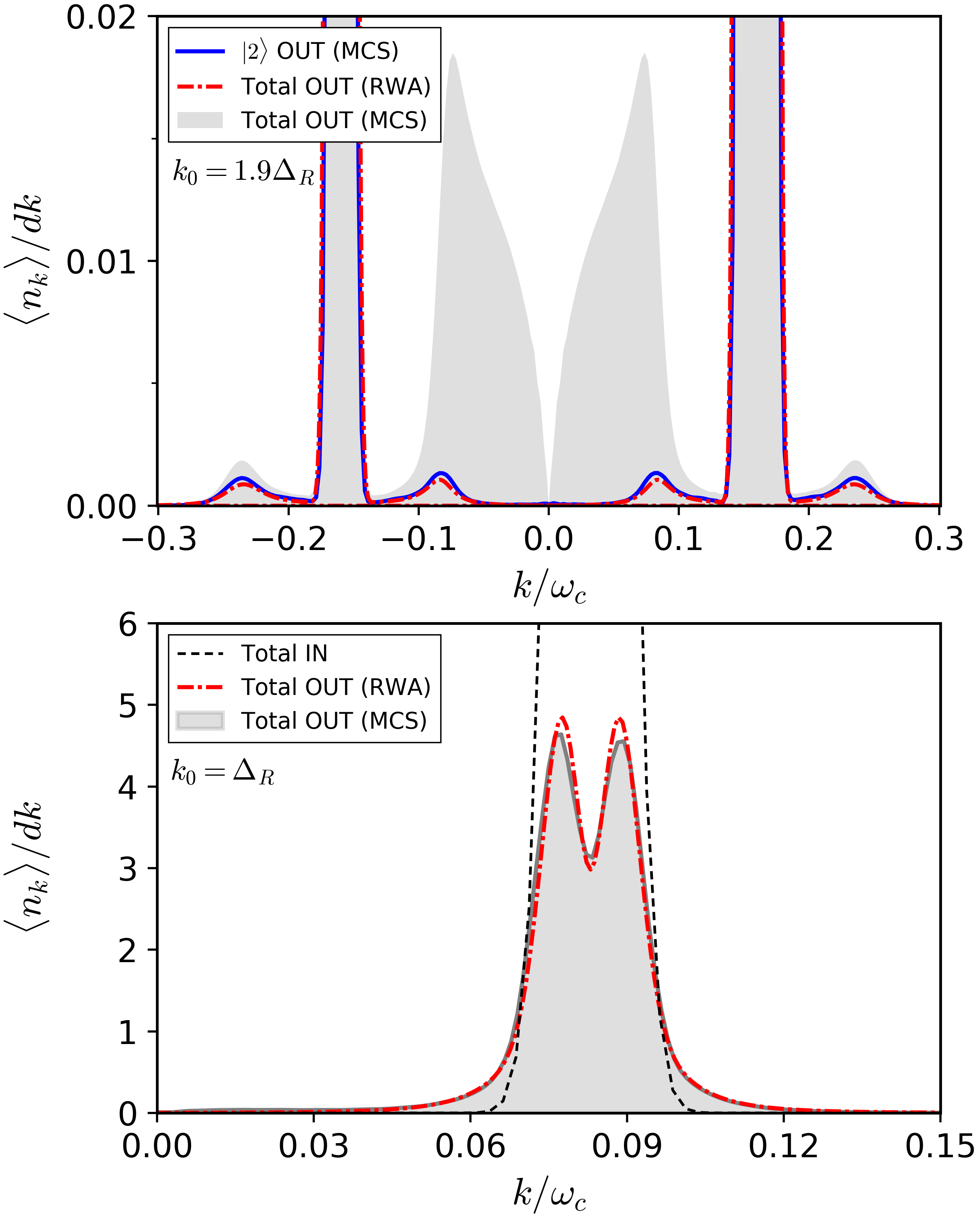
Figure 7: Comparison of MCS simulations to RWA input-output theory with regard to frequency conversion spectra for the off-resonant case (upper panel) and on-resonant case (lower panel). The parameters are the same as in Figs. 3 and 12. This confirms the previous interpretation that RWA inelastic processes dominate only on-resonance, and miss the main contributions to the off-resonant signal.

Comparison to the RWA power spectrum in the off-resonant and resonant cases is shown in the upper and lower panels of Fig. 7 respectively. In making this comparison, we used as input to the RWA calculation the numerically found renormalized level spacing and width, $\Delta_{R}$ and $\Gamma_{R}=\pi\alpha\Delta_{R}$, as this is essential to get the elastic peak correctly. The dominant inelastic process within the RWA is the scattering of two incoming photons into two outgoing photons, see panel (a) in Fig. 4. One sees that this process explains most of the total scattered spectrum in the resonant case. Indeed, the lower panel in Fig. 7 shows that the RWA and numerical MCS results are nearly identical on the scale shown. In particular both the overall width and shape of the inelastic power spectrum agree well. However, it is clear that the RWA prediction is only a small fraction of the total inelastic scattering in the off-resonant case (upper panel in Fig. 7), as particle production leads to qualitatively different and much larger cross-sections. Thus for these parameters, the RWA fails badly, even though the coupling constant $\alpha=0.1$ is not very large.

IV.2 Temporal correlations associated to particle production

It is interesting to study photon number temporal correlations, a standard measure of non-linearities, but now in light of the large inelastic effects that we uncovered in the ultra-strong coupling regime. We have computed the photon-number autocorrelation function $g_{2}(\tau)$ of the reflected signal ($x<0$, $k<0$), defined by

$$g_{2}(\tau)=\frac{\braket{a^{\dagger}_{x}a^{\dagger}_{x+\tau}a_{x+\tau}a_{x}}}{\braket{a^{\dagger}_{x+\tau}a_{x+\tau}}\braket{a^{\dagger}_{x}a_{x}}},$$ (27)

where $x$ is a point within the left-going wavepacket, such that both $x$ and $x+\tau$ are within the wavepacket. In principle, $g_{2}(\tau)$ also depends on $x$, but this dependence is weak provided the wavepacket is almost monochromatic, and the location $x$ is taken deep within the outgoing photon wavepacket. Details of the computation in the context of an MCS expansion are given in Appendix A.7.

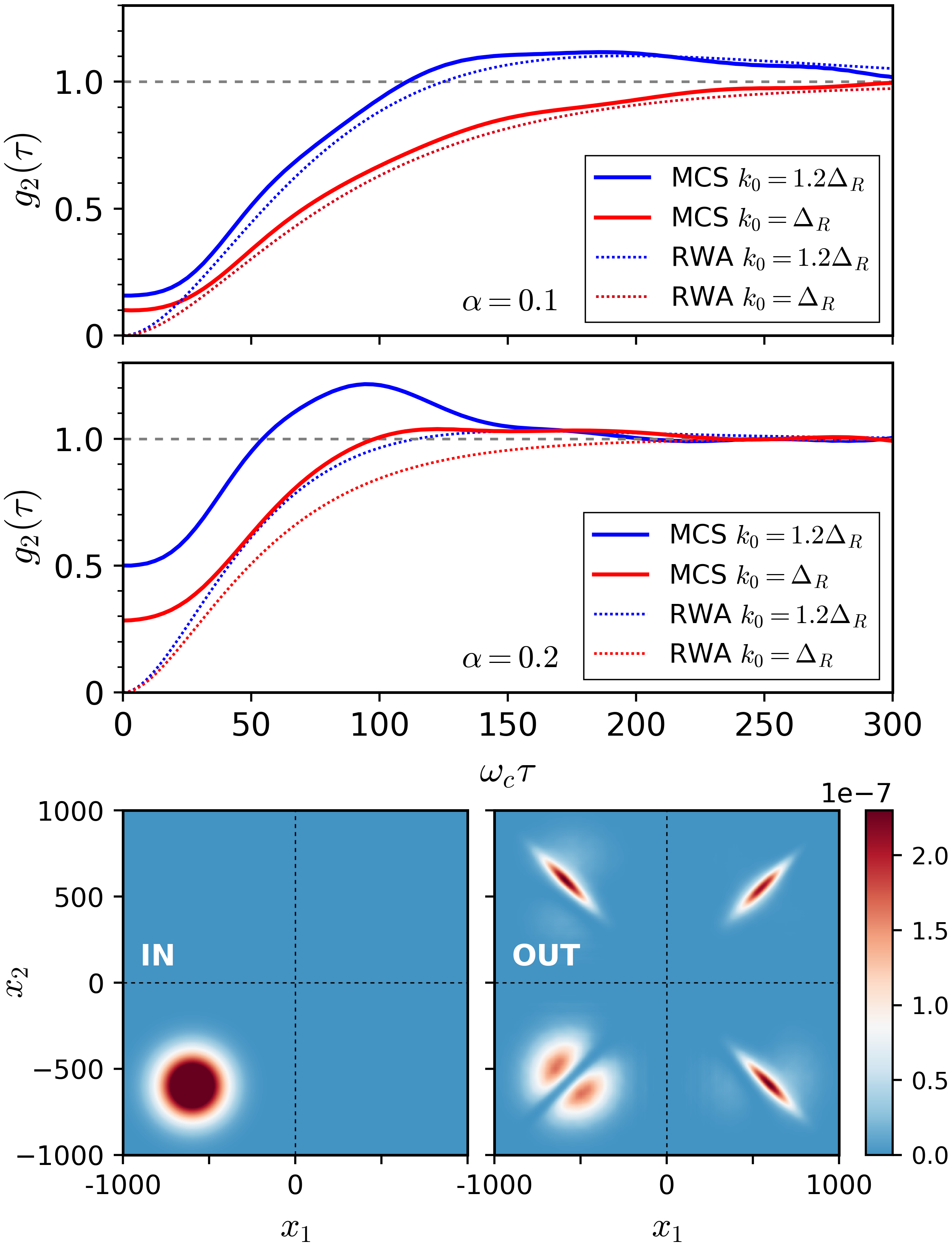
Figure 8: Second order correlation function $g_{2}(\tau)$ in reflection, at $\alpha=0.1$ (upper panel) and $\alpha=0.2$ (middle panel). The dip at $\tau=0$ is a standard signature of anti-bunching, but multiple photon emission seen in Fig. 3 at ultra-strong coupling leads to an incomplete cancellation, $g_{2}(0)>0$. In the off-resonant case ($k_{0}=1.2\Delta_{R}$), particle production is enhanced relative to the single photon reflection, resulting in a stronger bunching ($g_{2}(\tau)>1$) than predicted in the RWA. The MCS simulations were performed with the same parameters as in Fig. 12, except for the stronger coupling $\alpha=0.2$, $\sigma=0.004\omega_{c}$ and a hard cut-off that was used (see Appendix A.7). Bottom panel: Real space probability distribution of the two-photon states $|\alpha_{x_{1},x_{2}}|^{2}/dx^{2}$ at the initial (left panel) and final (right panel) times of the simulation. One remarks the absence of reflection for two photons arriving at the same time on the qubit, as seen by the dip within the probability distribution located in the bottom left quadrant of the right panel.

We find that temporal correlations are a very sensitive measure of ultra-strong coupling effects. In the resonant case (see the top panel of Fig. 8), the correlations are typical of single photon emission. The comparison to the RWA is globally quantitative, as expected from the previous agreement in the inelastic spectrum on-resonance (small oscillations at long time in $g_{2}(\tau)$ reflect the improper convergence of our MCS numerics near the edges of the outgoing wavepacket). In disagreement with the RWA however, we notice that the numerical data shows partial antibunching at zero delay, $g_{2}(0)>0$, signaling the production of particles, as was revealed by the low energy spectrum in Fig. 12. Thus particle production leads to physical effects that are potentially observable experimentally even when on resonance. This offset, which is zero in the RWA, is found to increase with $\alpha$ (see the upper middle of Fig. 8 for $k_{0}=\Delta_{R}$). The incomplete cancellation here can be readily interpreted as a probability of emitting many-photon states due to frequency down-conversion. Even more striking is the appearance of a large bunching signal at intermediate times in the off-resonant case (see the middle panel of Fig. 8 for $k_{0}=1.2\Delta_{R}$), which was not reported to our knowledge for the radiation of a single level qubit (bunching can be observed in spontaneous emission from multilevel atoms Sánchez-Burillo et al. (2016), due to a simpler cascade effect Gasparinetti et al. (2017), or from multiqubit systems Zheng and Baranger (2013); Laakso and Pletyukhov (2014); Fang and Baranger (2015)). Here, bunching originates from the single-shot emission of three photons by the two-level system, a property that is only allowed at ultra-strong coupling. The bunching signal becomes sizable in the off-resonant case, even though the particle production is comparable to that in the resonant case, because the reflection amplitude for single photon emission is reduced.

As a nice illustration of the partitioning of the incoming beam by the two-level system, we show in the bottom panels of Fig. 8 the real space probability distribution of the two-photon states $|\alpha_{x_{1},x_{2}}|^{2}/dx^{2}$ at the beginning and at the end of the time evolution. These results were obtained in the on resonant case with $\alpha=0.1$, by Fourier transforming to real space the $k$-space displacements. One can clearly see within the reflected signal (bottom left quadrant in the right panel) a deep trench on the diagonal $x_{1}=x_{2}<0$ with vanishing photon content (the incoming coherent state is shown in the bottom left panel for comparison). Two photons impinging simultaneously on the qubit have thus very low likelihood of both being reflected. This provides a direct visualization of photon anti-bunching, which arises because a single emitter can only reflect one photon at a time.

V Conclusion and perspectives

In this work we have developed a powerful methodology, namely the MCS technique, based on multi-mode and multi-configuration coherent state wavefunctions, to address many-body scattering properties of a two-level system that is embedded in a waveguide in the regime of ultra-strong coupling. This problem is intrinsically non-perturbative in nature due to the large production of particles, and cannot be reliably addressed by standard methods in quantum optics.

Our main finding is that excitation-preserving processes, described by the rotating wave approximation (RWA), dominate the inelastic spectrum only in the resonant situation. In contrast, when the frequency of the incoming photons is larger than the renormalized transition frequency of the two-level system, particle production becomes very favorable and dominates the inelastic signal.

We have been able to characterize precisely the output field, by decomposing the reflected and transmitted photon wavepackets into Fock states, and also by computing temporal correlations. The main results are as follows. (i) The process by which one photon is absorbed and three photons are emitted dominates in the off-resonant low power limit and leads to a broad spectrum of emission extending from zero frequency to the renormalized qubit frequency. (ii) Even in the resonant case, while the dominant inelastic emission near the resonant frequency is captured by the rotating wave approximation, there is still a broad spectrum of weak inelastic transmission produced by the counter-rotating terms. (iii) The correlation function $g_{2}(\tau)$ in reflection is a sensitive measure of ultra-strong coupling physics. In particular, particle production implies that it needs not vanish at zero delay, $g_{2}(0)>0$, and that it shows a strong bunching effect at a delay of order the inverse lifetime. (iv) Finally, we have found that perturbative predictions for the inelastic response Goldstein et al. (2013) cannot be used simply by renormalizing the bare qubit resonance frequency and linewidth when the coupling becomes ultrastrong. A more consistent theory including self-energy effects should be developed for the future.

All our quantitive predictions have relevance for the ongoing experimental effort in pushing waveguide quantum electrodynamics to the ultra-strong coupling regime. The connection to future experiments opens in addition various research directions. One important issue is that superconducting qubits are rarely operated as truly perfect two-level systems. Reducing the non-linearity of the qubit is typically important to minimize the effect of random noise from the circuit, but this strongly diminishes of course the amplitude of the interesting non-linear signals. Thus, extending our methodology to fully realistic superconducting quantum circuits will be crucial to address whether particle-production can be sizeable in practice.

The ability of the multi-coherent state method to deal naturally with coherent state pulses and open environments is also relevant for the large interest in quantum manipulation within complex architectures. It would thus be very useful to adapt techniques from signal treatment in order to numerically optimize the quantum evolution of the displacements that are used to simulate the Schrödinger dynamics of the complete system. Such developments will certainly be useful, because the description of strongly driven open quantum systems is a very important topic currently. Based on the physical artifacts that we can observe in our simulations of the scattering problem when the wavefunction is far from being converged, we suggest that the description of non-linear effects in quantum circuits for arbitrary pulse sequences is a very delicate subject that has to be examined with advanced and reliable many-body techniques.

Appendix A Technical aspects of the simulations

A.1 Dynamics of the MCS state vector

The multi-mode coherent state decomposition (7) leads to compact Euler-Lagrange equations (10) that determine the full quantum dynamics the spin-boson model (1):

$$P_{j} = \sum_{m}\left(\dot{p}_{m}-\frac{1}{2}p_{m}\kappa_{mj}\right)M_{jm},$$ (28)

$$F^{k}_{j} = \sum_{m}\left(p_{m}\dot{f}_{k,m}+\left(\dot{p}_{m}-\frac{1}{2}p_{m}\kappa_{mj}\right)f_{k,m}\right)M_{jm},$$ (29)

$$\kappa_{ij} = \sum_{k}\left(\dot{f}_{k,m}f^{\star}_{k,m}+\dot{f}^{\star}_{k,m}f_{k,m}-2f^{\star}_{k,j}\dot{f}_{k,m}\right).$$ (30)

Here, $M_{ij}=\braket{f_{i}}{f_{j}}={\rm e}^{-\frac{1}{2}\sum_{k}[|f_{k,i}|^{2}+|f_{k,j}|^{2}-2f_{k,i}^{*}f_{k,j}]}$ corresponds to the overlap between two multi-mode coherent states, and arises in the equations because of the over-completeness of the coherent state basis. Identical equations (up to a minus sign in all terms containing $g_{k}$) are obtained for the variables $q_{n}$ and $h_{k,n}$. We have denoted respectively in Eq. (28) and Eq. (29): $P_{j}=-i\frac{\partial E}{\partial p^{\star}_{j}}$ and $F^{k}_{j}=-i\frac{\partial E}{\partial f^{\star k}_{j}}-\frac{i}{2}\left(\frac{\partial E}{\partial p^{\star}_{j}}p^{\star}_{j}+\frac{\partial E}{\partial p_{j}}p_{j}\right)f^{k}_{j}$, with $E=\langle\Psi|H|\Psi\rangle$ the average energy, which reads explicitely:

$$E= \frac{\Delta}{2}\sum_{n,m}\Big{(}{p_{n}^{*}}q_{m}\langle f_{n}|h_{m}\rangle+p_{m}{q_{n}^{*}}\langle h_{n}|f_{m}\rangle\Big{)}$$

$$+\sum_{n,m}\Big{(}{p_{n}^{*}}p_{m}\langle f_{n}|f_{m}\rangle W_{nm}^{f}+{q_{n}^{*}}q_{m}\langle h_{n}|h_{m}\rangle W_{nm}^{h}\Big{)}$$

$$-\frac{1}{2}\sum_{n,m}\Big{(}{p_{n}^{*}}p_{m}\langle f_{n}|f_{m}\rangle L_{nm}^{f}-{q_{n}^{*}}q_{m}\langle h_{n}|h_{m}\rangle L_{nm}^{h}\Big{)},$$ (31)

where we have defined $W_{nm}^{f}=\sum_{k>0}\omega_{k}f_{k,n}^{*}f_{k,m}$, $W_{nm}^{h}=\sum_{k>0}\omega_{k}h_{k,n}^{*}h_{k,m}$, $L_{nm}^{f}=\sum_{k>0}g_{k}(f_{k,n}^{*}+f_{k,m})$, $L_{nm}^{h}=\sum_{k>0}g_{k}(h_{k,n}^{*}+h_{k,m})$. We now proceed with the implementation of a new and efficient numerical solution of the dynamical equations.

A.2 New integration algorithm

One can note that the dynamical equation (29) for the displacement field $f_{k,m}(t)$ is not yet in the proper form where a unique time derivative $\dot{f}_{k,m}(t)$ is extracted on one side of the set of equations. Achieving such a decomposition is required for efficient time integration, but considering that the system under study will require $N_{\mathrm{modes}}\simeq 1000$ (for accurate spectral resolution) and $N_{\mathrm{cs}}\simeq 40$ (for convergence of the quantum many-body state), a brute force inversion of equations (28-29) would scale prohibitively as $(N_{\mathrm{cs}}\times N_{\mathrm{modes}})^{3}$ operations for each time step. A more efficient algorithm, allowing to cope with a few hundred modes was proposed in Ref. Gheeraert et al. (2017), used an inversion technique with only $(N_{\mathrm{cs}})^{6}$ operations, which is favorable provided $N_{\mathrm{cs}}\ll N_{\mathrm{modes}}$. We present here an improved version of this algorithm, which enables us to reach the realistic situation of several thousands of modes.

The first step is to multiply Eq. (28) by $M^{-1}$, with $M$ the overlap matrix $M_{ij}=\braket{f_{i}}{f_{j}}$:

$$\sum_{j}M^{-1}_{nj}P_{j} = \dot{p_{n}}-\frac{1}{2}\sum_{mj}p_{m}\kappa_{mj}M^{-1}_{mj}M_{jn}$$ (33)

$$= \dot{p_{n}}-\frac{1}{2}p_{n}\sum_{q}(\dot{f}_{q,m}f^{\star}_{q,m}+\dot{f}^{\star}_{q,m}f_{q,m})$$

$$+\sum_{mjq}p_{m}M^{-1}_{nj}M_{jm}f^{\star}_{q,j}\dot{f}_{q,m},$$

and similarly for Eq. (29):

$$\sum_{j}M^{-1}_{nj}F^{k}_{j} = p_{n}\dot{f}_{k,n}+\dot{p}_{n}f_{k,n}$$ (34)

$$-\frac{1}{2}p_{n}f_{k,n}\sum_{q}(\dot{f}_{q,n}f^{\star}_{q,n}+\dot{f}^{\star}_{q,n}f_{q,n})$$

$$+\sum_{jmq}p_{m}M^{-1}_{nj}M_{jm}f_{k,m}f^{\star}_{q,j}\dot{f}_{q,m}.$$

We now substitute Eq. (33) in Eq. (34):

$$p_{n}\dot{f}_{k,n} = \sum_{j}(M^{-1}_{nj}F^{k}_{j}-f_{k,n}M^{-1}_{nj}P_{j})$$

$$-\sum_{mjq}M^{-1}_{nj}M_{jm}p_{m}f^{\star}_{q,j}\dot{f}_{q,m}\left(f_{k,m}-f_{k,n}\right),$$

which allowed to eliminate the complex conjugate time derivative $\dot{f}^{\star}_{q,m}$. Eq. (A.2) is not yet in explicit form since time derivatives of all possible displacement fields appear in the right hand side. We define the mode-independent quantities $a_{in}=p_{n}\sum\limits_{k}f^{\star}_{k,i}\dot{f}_{k,n}$ and $b_{in}=\sum\limits_{k}f^{\star}_{k,i}f_{k,n}$ and solve for $a_{in}$ by inserting Eq. (A.2) in its expression:

$$a_{in}+\sum_{mj}a_{jm}M^{-1}_{nj}M_{jm}\left(b_{im}-b_{in}\right) = A_{in},$$ (36)

with $A_{in}=\sum_{jk}f^{\star}_{k,i}\left(M^{-1}_{nj}F^{k}_{j}-f_{k,n}M^{-1}_{nj}P_{j}\right)$.

After solving the linear system (36) with the $(N_{\mathrm{cs}})^{2}$ unknown parameters $a_{in}$, the evolution equation for each displacement field is then cast into explicit form:

$$p_{n}\dot{f}_{k,n} = \sum_{jk}(M^{-1}_{nj}F^{k}_{j}-f_{k,n}M^{-1}_{nj}P_{j})$$ (37)

$$-\sum_{mj}M^{-1}_{nj}M_{jm}a_{jm}(f_{k,m}-f_{k,n}),$$

which can be integrated numerically using an RK4 method. The numerical inversion of the system (36) can be sped up below the naive $(N_{\mathrm{cs}})^{6}$ cost by defining $d_{in}=\sum_{j}M^{-1}_{nj}M_{jm}a_{jm}$ and $\alpha_{inm}=\sum_{l}M^{-1}_{in}M_{ln}(b_{lm}-b_{ln})$, so that we can solve a linear system for $d_{in}$:

$$\sum_{mj}\left(\delta_{ij}\delta_{nm}+\alpha_{inm}\delta_{nj}\right)d_{mj}=\sum_{j}M^{-1}_{nj}M_{jm}A_{jm}$$ (38)

which assumes a sparse form suitable for Krylov based methods (provided a good preconditioner can be found).

A.3 Incoming and outgoing many-body states

Combining the incoming coherent state, described by the displacement $z_{k}$ in Eq. (13), with the static polarization cloud wavefunction Eq. (11) can be done by transforming the incoming signal in the even/odd basis (see Sec. II.3). For the spin-up projection of the wavefunction, we readily find:

$$\ket{\Psi_{\uparrow}} =D(z^{e})D(z^{o})\ket{\Psi^{\mathrm{GS}}_{\uparrow}}$$ (39)

$$=e^{\sum_{k>0}z_{k}^{e}a_{k}^{e\dagger}-c.c.}\sum_{m}^{{N^{\mathrm{GS}}_{\textrm{cs}}}}p^{\mathrm{GS}}_{m}e^{\sum_{k>0}f_{k,m}^{\mathrm{GS}}a_{k}^{e\dagger}-c.c.}\ket{0}_{e}\ket{z^{o}}_{o}$$

which can be recombined using the standard relation $e^{A}e^{B}=e^{A+B}e^{\frac{1}{2}[A,B]}$, valid as the commutator here is only a number. The initial state associated to the $\uparrow$ qubit state thus reads:

$$\ket{\Psi_{\uparrow}} = \sum_{m}^{{N^{\mathrm{GS}}_{\textrm{cs}}}}p^{\mathrm{GS}}_{m}e^{\frac{1}{2}\sum_{k>0}\left(z_{k}^{e}f_{k,m}^{\mathrm{GS}*}-z_{k}^{e*}f_{k,m}^{\mathrm{GS}}\right)}$$

$$\times\,e^{\sum_{k>0}\left[\left(f_{k,m}^{\mathrm{GS}}+z_{k}^{e}\right)a_{k}^{e\dagger}-\left(f_{k,m}^{\mathrm{GS}}+z_{k}^{e}\right)^{*}a_{k}^{e}\right]}\ket{0}_{e}\ket{z^{o}}_{o}.$$

For the spin-down projection, one simply replaces $f_{k,m}^{\mathrm{GS}}$ by $-f_{k,m}^{\mathrm{GS}}$ without changing the sign of $z_{k}^{e}$, so that our total initial wavefunction is given by Eq. (17).

The outgoing wavepacket is constructed in a similar spirit:

$$\ket{\Psi^{\mathrm{OUT}}}=\sum_{m=1}^{{N^{\mathrm{OUT}}_{\textrm{cs}}}}p^{\mathrm{OUT}}_{m}e^{\frac{1}{2}\sum_{x>0}\left(f_{x,m}^{\mathrm{OUT}}a_{x}^{\dagger}-f_{x,m}^{\mathrm{OUT}*}a_{x}\right)}\ket{0},$$ (41)

where we have written the displacements of the outgoing state in real space because they have no spatial overlap with the real space modes that populate the many-body ground state (working in momentum space would complicate the analysis). This decoupling occurs in fact when the wavepacket reaches distances away from the qubit that are larger than the inverse Kondo energy Snyman and Florens (2015), or said otherwise, that are larger than the entanglement cloud around the qubit. Clearly the quantum many-body character of the scattering process is encoded in the sum over more than a unique coherent state, in contrast to the incoming wavepacket (16) that is characterized by a single coherent state (namely a classical-like signal). Contrarily to the driven dynamics for an isolated few level quantum system, this long time equilibration between the many-body ground state and the wavepacket is physically expected because the waveguide acts as a bath for the dressed two-level system, and thus provides a natural pathway for relaxation, even in a many-body system.

Extracting the wavepacket contribution (41) from the long-time wavefunction (18) can be performed as follows. The complete set of displacements $\{f_{k,n}^{e}(T),h_{k,n}^{e}(T)\}$ in the even sector at a fixed long time $T$ for the full wavefunction (7) are first Fourier transformed to real space using (12). The local photon density $n(x)$ associated to these displacements is sketched in Fig. 1: photons are either bound statically near the qubit (associated to the dressed vacuum) or travel in the outgoing wavepackets. The displacements are then simply set to zero in the region surrounding the qubit, and Fourier transformed back to the momentum basis. Due to factorization (18), the outgoing wavefunction is recovered, up to a normalization factor, which is supplemented accordingly. The even modes thus obtained and the trivial odd mode wavefunctions are finally combined together in the case of the incoming wavepacket, allowing reconstruction of the full outgoing wavefunction for the physical waveguide.

A.4 Convergence properties

Assessing the good convergence of the numerical results is important to gain confidence in the time-dependent variational MCS technique Indeed, we find that using too few variational parameters imposes strong constraints on the dynamics, which may result in unphysical behavior and numerical artifacts. One delicate test is the strong power saturation spectrum shown in Fig. 2 of the main text. Indeed, the calculations that use only a single coherent state, as done in a previous publication Bera et al. (2016), are found to be problematic in the strong power regime. This behavior is illustrated in the top panel of Fig. 9, showing the power reflection spectrum as a function of incoming frequency at a strong input power ($\bar{n}=2$) for three different values of the number of coherent states $N_{\mathrm{cs}}=1,4,16$. The computation with $N_{\mathrm{cs}}=1$ is indeed quite noisy and imprecise, and a smooth and converged curve is only obtained at $N_{\mathrm{cs}}=16$. We find that the inelastic spectra shown in Fig. 3 are also delicate to compute, because they consist of a tiny fraction of the total signal, and encode complex quantum states. A relatively large number of coherent state is also necessary here for success, even at small input power.

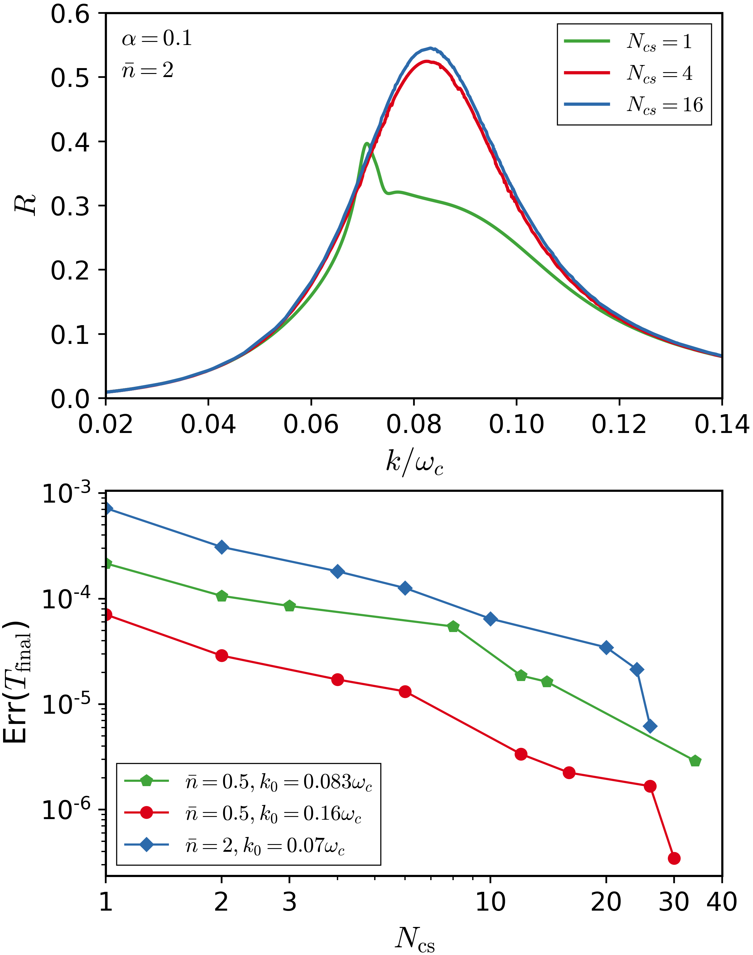
Figure 9: Top panel: Power reflection spectrum shown for different number of coherent states $N_{\mathrm{cs}}=1,4,16$ included in the MCS wavefunction (7), with the same parameters as in Fig. 2 in the case of $\bar{n}=2$ photons in the incoming beam. Bottom panel: Convergence of the error defined in the text at the final time $T_{\rm{final}}$ of the simulations, as a function of coherent state number in the wavefunction for various incoming momenta and power.

An unbiased criterion for the convergence of our algorithm for this non-equilibrium many-body dynamics is also shown in the lower panel of Fig. 9. Here we demonstrate that the error with respect to the exact Schrödinger dynamics vanishes with the number of coherent states. The error is defined Gheeraert et al. (2017) by the squared norm

$$\mathrm{Err}(t)\equiv\big{<}\Phi(t)|\Phi(t)\big{>}$$ (42)

of the auxiliary state $|\Phi(t)\big{>}\equiv(i\partial_{t}-H)|\Psi(t)\big{>}$. Indeed, this error decreases steadily and scales as $[N_{\textrm{cs}}]^{-2}$. For the off-resonant case of Fig. 3 (see bottom curve in the lower panel of Fig. 9) we managed to reach an error of the order of $10^{-7}$.

A.5 Protocol for adding coherent states during the time evolution

Because the coherent state basis is over-complete, all the coherent states required for good convergence (typically $N_{\mathrm{cs}}>16$) cannot be initialised simultaneously at the initial time. Indeed, two coherent states with identical displacements will result in a singularity in the matrices to be inverted for solving the dynamics, due to a vanishing determinant. During the initial stage of the dynamics, this is not an issue, as only a small number of coherent states (typically 6 to 10) is needed to describe the static many-body cloud and the incoming coherent state. After some time however, the wavepacket starts to interact with the dressed qubit, which would increase the error should the number of coherent states remain the same. Therefore, to account for the emerging complexity of the many-body scattered state, we progressively increase the number of coherent states $N_{\textrm{cs}}$ in the MCS state vector (Eq. (7)), initializing the newly added coherent states in a bosonic vacuum configuration with zero weight. Thus, the addition of a new set of variational displacement does not immediately affect the dynamics, but provides the necessary freedom to our variational algorithm for maintaining a minimal error at later times. This procedure is illustrated in Fig. 10.

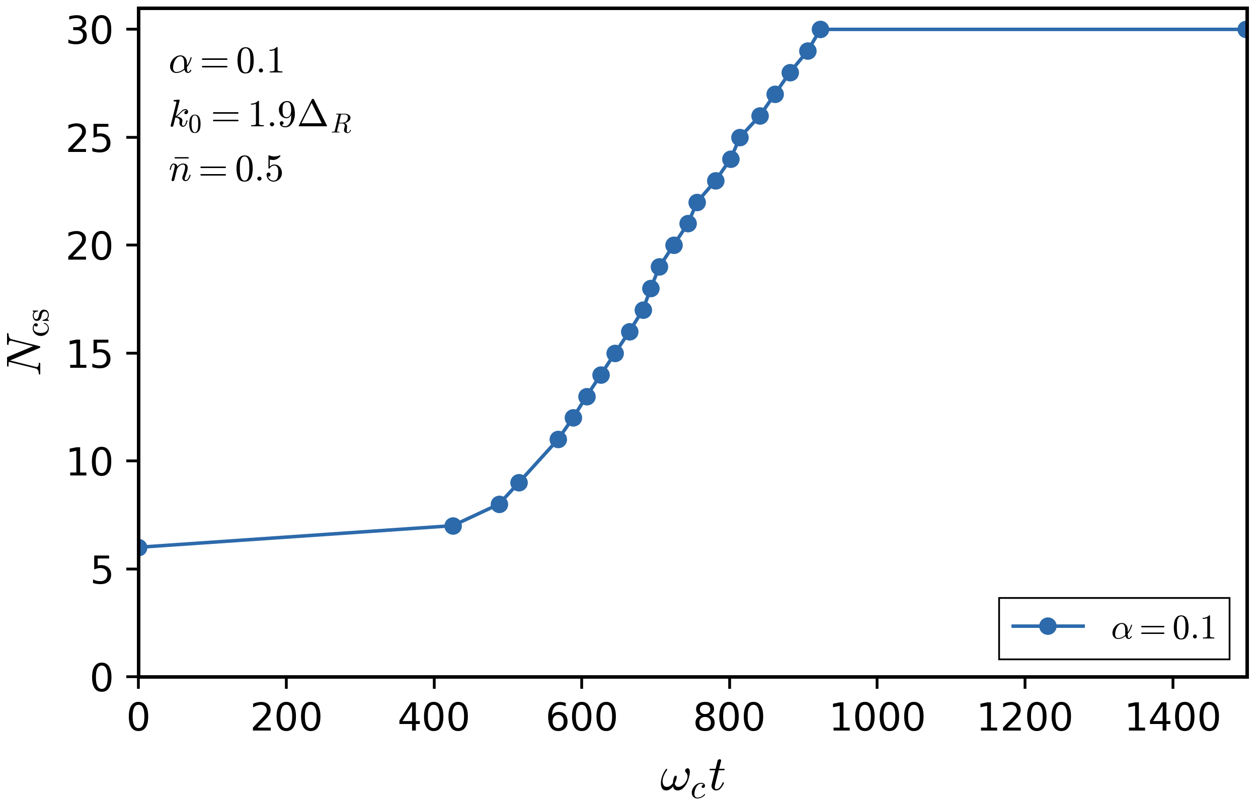
Figure 10: Number of used coherent states in the MCS wave-function defined in Eq. (7) as a function of time, for the off-resonant $k_{0}=0.16\omega_{c}$ simulation. The initial 6 coherent states present are those required for describing the dressed ground state of the spin-boson model as well as the incoming wave-packet. Subsequent additions of coherent states start only as the wave-packet starts to impinge on the qubit. The addition process stops as the wavepackets exit the interaction region.

The right time for a coherent state to be added is found by monitoring the error, which was defined by Eq. (42), and by defining an error increment $\mathrm{Err}_{\mathrm{max}}$ at which the coherent state should be added. Whenever $\mathrm{Err}(t)-\mathrm{Err}_{\mathrm{ref}}>\textrm{Err}_{\mathrm{max}}$ during the time evolution, where Err_ref is the error right after the previous coherent state was added, one simply adds a coherent state with displacement $f_{m}^{k}=h_{m}^{k}=0$ and weights $p_{m}=q_{m}\simeq 10^{-6}$ in Eq. (7). The near-zero amplitude ensures that this new coherent state only changes the wave-function negligibly at the time it is added. Empirically, we find the value of $\mathrm{Err}_{\mathrm{max}}=10^{-7}$ to be adequate. The system, through the variational principle, will subsequently have the possibility to increase the displacements and weights according to the requirements of the quantum trajectory. As an example, a plot of the number of coherent states as a function of time for the off-resonant $k_{0}=0.16\omega_{c}$ simulation in Fig. 3 is given in Fig. 10.

A.6 Calculation of Number Resolved Spectra

To assess the nature of particle production in the scattering process, we analyze the inelastic spectrum in terms of Fock states $\ket{N}$. First, consider the general expansion of the multi-mode outgoing wavefunction (19) in terms of number states:

$$\ket{\Psi^{\mathrm{OUT}}} = \gamma\ket{0}+\sum_{k}\alpha_{k}a_{k}^{\dagger}\ket{0}+\sum_{k_{1},k_{2}}\alpha_{k_{1},k_{2}}a_{k_{1}}^{\dagger}a_{k_{2}}^{\dagger}\ket{0}$$ (43)

$$+\sum_{k_{1},k_{2},k_{3}}\alpha_{k_{1},k_{2},k_{3}}a_{k_{1}}^{\dagger}a_{k_{2}}^{\dagger}a_{k_{3}}^{\dagger}\ket{0}+\ \ \mathrm{...}$$

It can then easily be verified that the 1-photon amplitude is given by:

$$\alpha_{k}=\bra{0}a_{k}\ket{\Psi^{\mathrm{OUT}}}=\sum_{n}p_{n}f_{k,n}\braket{0}{f_{n}},$$ (44)

and that the scattering amplitude for a generic $N$-photon state is:

$$\alpha_{k_{1},...,k_{N}}=\frac{1}{N!}\bra{0}a_{k_{1}}...\ a_{k_{N}}\ket{\Psi^{\mathrm{OUT}}},$$ (45)

which can be obtained straightforwardly from the algebraic identities of coherent states. For the sake of clarity, we have dropped the OUT labels on $p_{n}$ and $f_{n,k}$. From the multi-photon amplitudes, we can then compute the probability distribution for finding a photon in a given $k$ mode, according to the various Fock contents of the total wavefunction:

$$\braket{n_{k}}_{\mathrm{1photon}} = |\alpha_{k}|^{2},$$

$$\braket{n_{k}}_{\mathrm{2photon}} = 4\sum_{k1}|\alpha_{k,k1}|^{2},$$

$$\braket{n_{k}}_{\mathrm{3photon}} = 18\sum_{k2,k3}|\alpha_{k,k2,k3}|^{2}.$$ (46)

These Fock resolved inelastic contributions $\braket{n_{k}}_{\mathrm{Nphoton}}$, with $N=2,3,4$ are displayed as full lines in Fig. 3 (note that the outgoing $N=1$ process is purely elastic and is not shown).

A.7 Calculation of $g_{2}(\tau)$

In this appendix, we give some details on the calculation of the correlation function $g_{2}(\tau)$ when using the MCS approach. First, since we take the speed of light $c=1$, $\tau$ is just the distance traveled by radiation in time $\tau$. Inserting the MCS expansion Eq. (7) into definition (27), we obtain a compact expression for the autocorrelation function in terms of the real space displacements $f_{n}^{x}$:

$$g_{2}(\tau)=\frac{\sum_{m,n}p_{n}^{*}p_{m}(f^{x}_{n})^{*}(f^{x+\tau}_{n})^{*}f^{x+\tau}_{m}f^{x}_{m}\braket{f_{n}}{f_{m}}}{\braket{n(x)}\braket{n(x+\tau)}},$$ (47)

with the local photon number

$$\braket{n(x)}=\braket{a^{\dagger}_{x}a_{x}}=\sum_{m,n}p_{n}^{*}p_{m}(f^{x}_{n})^{*}f^{x}_{m}\braket{f_{n}}{f_{m}}.$$ (48)

In the simulations performed to compute this quantity we used a sharp cutoff $\Theta(\omega_{c}-\omega)$ for the dispersion relation instead of the exponential cutoff $\rm{e}^{-\omega/\omega_{c}}$ which we defined in Eq. (5). Note that using the hard cut-off results in a slightly lower value of the renormalised qubit energy $\Delta_{R}$, than with the exponential cutoff. This allowed us to decrease the numerical cost and therefore attain a higher number of coherent states, $N_{\rm{cs}}=40$, which was necessary because second-order correlations are more challenging to converge than average photon numbers. The simulations were stopped at a timescale $T=1250/\omega_{c}$ long enough that the wavepacket is located far away from the dressed qubit, and we chose the spacial point $x=-681$ in Eq. (27), so as to keep the range of the function near the center of the wavepacket. We finally note that spurious effects associated with the finite spatial extension of the wavepacket (due to $\sigma\neq 0$) lead to the small oscillations seen in Fig. 8 at longer times.

Appendix B Further analysis of non-linear emission

B.1 Detailed off-resonant conversion spectra

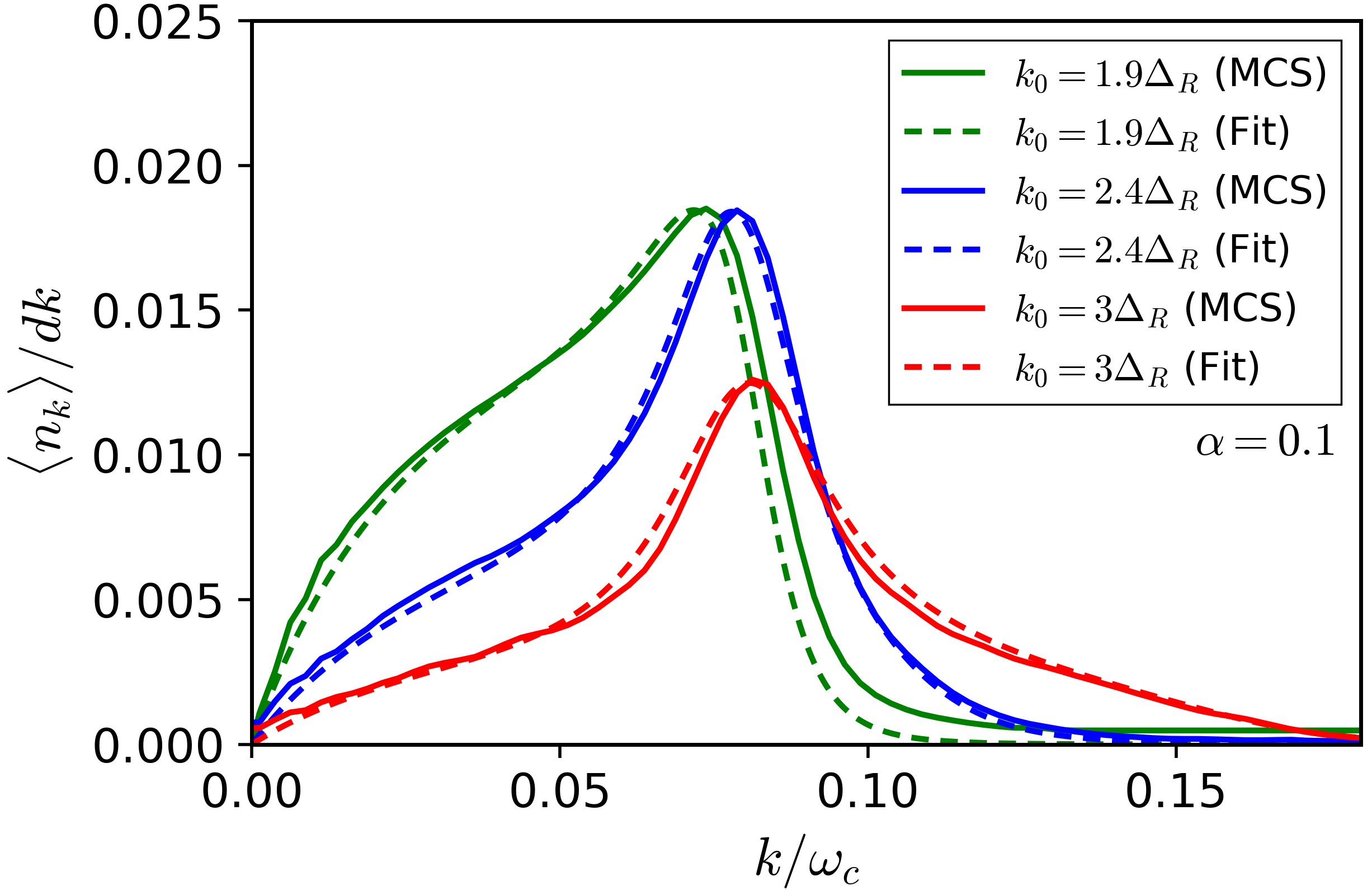
Figure 11: Low-energy inelastic spectrum for several off-resonant values of the incoming momentum $k_{0}=0.16,0.20,0.25\omega_{c}$ obtained using the MCS technique (with the same parameters as in Fig. 3), together with a comparison to the analytical formula (B.1), using a fitted and momentum-dependent linewidth $\gamma_{R}(k_{0})$.

We proceed here with a systematic study of particle production spectra in the off-resonant case, as a function of incoming momentum $k_{0}$ (see Fig. 11). A weak coupling calculation of the one photon to three photon conversion process (see Fig. 4) was given in the $\alpha\to 0$ limit in Ref. Goldstein et al. (2013). We have found that this theory can quantitatively account for our data at small $\alpha$ upon two important modifications. First, as already seen by the frequency shift in the reflection spectrum in Fig. 2, one must replace the bare qubit frequency $\Delta$ by the renormalized quantity $\Delta_{R}$ within the analytical results given by the perturbative approach. Second, the golden rule value for the qubit linewidth appearing in the transmission lineshape, given by $\Gamma=\pi\alpha\Delta$ at small $\alpha$, cannot be used. For the elastic response, one can use reliably $\Gamma_{R}=\pi\alpha\Delta_{R}$ up to moderate values of $\alpha$. However, we find that the renormalized broadening parameter $\gamma_{R}^{\mathrm{inel}}$ entering the inelastic response function for fixed value of the incoming momentum $k_{0}$ is not given by $\Gamma_{R}$, but rather displays a strong momentum dependence, $\gamma_{R}^{\mathrm{inel}}=\gamma_{R}(k_{0})$. This is not completely unexpected, since a consistent calculation should include the full momentum variation of the self-energy, and we found that the theory of Ref. Goldstein et al. (2013) is very sensitive to the way the inelastic regularization is implemented. For the present purpose, we will only use a phenomelogical model that uses (as fitting parameters) only two renormalized quantities $\Delta_{R}$ and $\gamma_{R}(k_{0})$ within the perturbative formula:

$$\braket{n_{k}}_{\mathrm{3photon}} = \frac{\alpha^{4}}{8}\Delta_{R}^{2}\int_{0}^{k_{0}-k}\!\!\!\!\!\mathrm{d}k_{1}\;kk_{0}k_{1}k_{2}$$

$$\Big{|}\frac{k_{0}kk_{1}k_{2}-k_{\Delta}^{2}(k^{2}+k_{1}^{2}+k_{2}^{2}+kk_{1}+kk_{2}+k_{1}k_{2})+3k_{\Delta}^{4}}{(k^{2}-k_{\Delta}^{2})(k_{0}^{2}-k_{\Delta}^{2})(k_{1}^{2}-k_{\Delta}^{2})(k_{2}^{2}-k_{\Delta}^{2})}\Big{|}^{2},$$

with $k_{2}=k_{0}-k_{1}-k$ and $k_{\Delta}=\Delta_{R}+i\gamma_{R}(k_{0})$, with $\Delta_{R}$ the renormalized qubit frequency and $\gamma_{R}(k_{0})$ the linewidth describing the inelastic spectrum, which is fitted from our numerical data. The resulting comparison is shown in Fig. 11, with excellent quantitative agreement.

B.2 Detailed on-resonant conversion spectra

We consider here the detailed photonic content of the emission spectra in the resonant case where the incoming photon energy $k_{0}=\Delta_{R}$ matches the renormalized atomic transition energy. Fig. 12 shows the total transmitted signal as well as its decomposition in terms of number states with $N=1,2,3$ photons. Not surprisingly, the two-photon amplitude in this regime is strongly enhanced with respect to the off-resonant situation of Fig. 3. One-photon contributions are also observed as two side-bands away from the resonance $\Delta_{R}$, which are due to the finite width of the incoming wave-packet. The resonant 1-photon states (at exactly $k=k_{0}$) are completely reflected, as expected. In the resonant case, $2\to 2$ RWA frequency conversion gives rise to the broader wings (extending clearly beyond the linewidth $\sigma$ of the pump), as seen in the $N=2$ curve of Fig. 12. As in the off-resonant case, the resonant scattered spectrum also presents a 3-photon low energy continuum, as can be seen from the inset. The shape however does not present any sharply peaked feature, since this time the continuum does not contain the resonant frequency $k=\Delta_{R}$ at which the qubit spontaneously reemits. Instead, the spectrum is more flat, implying the single photon splits more uniformly into all the possible $(k_{1},k_{2},k_{3})$ allowed by the $1\to 3$ process of Fig. 4. Interestingly, the magnitude of this 3-photon continuum is of the same order of magnitude as in the off-resonant case of Fig. 3, since non-linear processes are here intensified by having an on-resonant input, which compensates for the absence of an enhancing resonant frequency in the output below $k_{0}$. Again, this particle production process dominates the RWA contribution, here only away from the probe frequency.

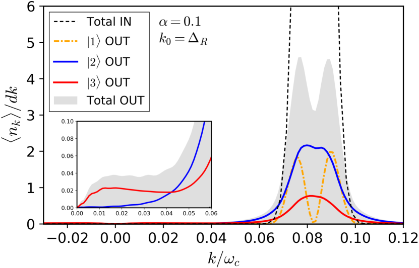
Figure 12: On-resonance transmission spectrum for an incoming photon energy that matches the renormalized qubit excitation, $k_{0}=0.08\omega_{c}=\Delta_{R}$. The simulation required 2500 modes with the use of 34 coherent states (all other parameters are identical to the ones in Fig. 3). The black dashed curve corresponds to the nearly monochromatic incoming wave-packet. Because of the wavepacket finite linewidth $\sigma$, a small fraction of one-photon states is still transmitted (dot-dashed line), despite being on resonance. The two-photon contribution (top full line) presents wider inelastic wings, that extend beyond the width $\sigma$, and that are parametrically larger in amplitude than the off-resonant signal of Fig. 3. The 3-photon continuum is magnified in the inset.

References

- Haroche and Raimond (2006) S. Haroche and J.-M. Raimond, Exploring the Quantum (Oxford Univ. Press, Oxford, UK, 2006).
- Meystre and Sargent (2010) P. Meystre and M. Sargent, Elements of quantum optics (Springer-Verlag Berlin, Heidelberg, 2010).
- Loudon (2003) R. Loudon, The Quantum Theory of Light, 3rd ed. (Oxford University Press, New York, 2003).
- Eikema et al. (2001) K. S. E. Eikema, J. Walz, and T. W. Hänsch, “Continuous coherent lyman- excitation of atomic hydrogen,” Phys. Rev. Lett. 86, 5679–5682 (2001).
- Mabuchi and Doherty (2002) H. Mabuchi and A. C. Doherty, “Cavity quantum electrodynamics: Coherence in context,” Science 298, 1372–1377 (2002).
- Haroche (2013) Serge Haroche, “Nobel Lecture: Controlling photons in a box and exploring the quantum to classical boundary,” Rev. Mod. Phys. 85, 1083–1102 (2013).
- Hartmann (2016) Michael J. Hartmann, “Quantum simulation with interacting photons,” J. Opt. 18, 104005 (2016).
- Haapamaki et al. (2016) C.M. Haapamaki, J. Flannery, G. Bappi, Maruf R. Al, S.V. Bhaskara, O. Alshehri, T. Yoon, and M. Bajcsy, “Mesoscale cavities in hollow-core waveguides for quantum optics with atomic ensembles,” Nanophotonics 5, 392–408 (2016).
- Solano et al. (2017) Pablo Solano, Jeffrey A. Grover, Jonathan E. Hoffman, Sylvain Ravets, Fredrik K. Fatemi, Luis A. Orozco, and Steven L. Rolston, “Optical nanofibers: A new platform for quantum optics,” in Advances In Atomic, Molecular, and Optical Physics, Vol. 66, edited by Ennio Arimondo, Chun C. Lin, and Susanne F. Yelin (Academic Press, 2017) pp. 439–505.
- Roy et al. (2017) Dibyendu Roy, C. M. Wilson, and Ofer Firstenberg, “Colloquium: Strongly interacting photons in one-dimensional continuum,” Rev. Mod. Phys. 89, 021001 (2017).
- Forn-Díaz et al. (2017) P. Forn-Díaz, J. J. García-Ripoll, B. Peropadre, J.-L. Orgiazzi, M. A. Yurtalan, R. Belyansky, C. M. Wilson, and A. Lupascu, “Ultrastrong coupling of a single artificial atom to an electromagnetic continuum in the nonperturbative regime,” Nat. Phys. 13, 39 (2017).
- Puertas Martínez et al. (2018) J. Puertas Martínez, S. Léger, N. Gheereart, R. Dassonneville, N. Planat, F. Foroughi, Y. Krupko, O. Buisson, C. Naud, W. Guichard, S. Florens, S. Snyman, and N. Roch, “Probing a transmon qubit via the ultra-strong coupling to a josephson waveguide,” arXiv preprint arXiv:1802.00633 (2018).
- Gu et al. (2017) X. Gu, A. Frisk Kockum, A. Miranowicz, Y.-X. Liu, and F. Nori, “Microwave photonics with superconducting quantum circuits,” Phys. Rep. 718, 1 (2017).
- Devoret et al. (2007) M. Devoret, S. Girvin, and R. Schoelkopf, “Circuit-QED: How strong can the coupling between a josephson junction atom and a transmission line resonator be?” Ann. Phys. (Leipzig) 16, 767 (2007).
- Schoelkopf and Girvin (2008) R. Schoelkopf and S. M. Girvin, “Wiring up quantum systems,” Nature 451, 664 (2008).
- Bourassa et al. (2009) J. Bourassa, J. M. Gambetta, A. A. Abdumalikov, O. Astafiev, Y. Nakamura, and A. Blais, “Ultrastrong coupling regime of cavity QED with phase-biased flux qubits,” Phys. Rev. A 80, 032109 (2009).
- Niemczyk et al. (2010) T. Niemczyk, F. Deppe, H. Huebl, E. P. Menzel, F. Hocke, M . J. Schwarz, J. J. García-Ripoll, D. Zueco, T. Hümmer, E. Solano, A. Marx, and R. Gross, “Circuit quantum electrodynamics in the ultrastrong-coupling regime,” Nat. Phys. 6, 772 (2010).
- Forn-Díaz et al. (2010) P. Forn-Díaz, J. Lisenfeld, D. Marcos, J. J. García-Ripoll, E. Solano, C. J. P. M. Harmans, and J. E. Mooij, “Observation of the bloch-siegert shift in a qubit-oscillator system in the ultrastrong coupling regime,” Phys. Rev. Lett. 105, 237001 (2010).
- Yoshihara et al. (2017) F. Yoshihara, T. Fuse, S. Ashhab, K. Kakuyanagi, S. Saito, and K. Semba, “Superconducting qubit-oscillator circuit beyond the ultrastrong-coupling regime,” Nat. Phys. 13, 44 (2017).
- Astafiev et al. (2010) O. Astafiev, A. M. Zagoskin, A. A. Jr Abdumalikov, Y. A. Pashkin, T. Yamamoto, K. Inomata, Y. Nakamura, and J. S. Tsai, “Resonance fluorescence of a single artificial atom,” Science 327, 840 (2010).
- Abdumalikov et al. (2011) A. A. Abdumalikov, O. V. Astafiev, Yu. A. Pashkin, Y. Nakamura, and J. S. Tsai, “Dynamics of coherent and incoherent emission from an artificial atom in a 1d space,” Phys. Rev. Lett. 107, 043604 (2011).
- Hoi et al. (2011) Io-Chun Hoi, C. M. Wilson, Göran Johansson, Tauno Palomaki, Borja Peropadre, and Per Delsing, “Demonstration of a single-photon router in the microwave regime,” Phys. Rev. Lett. 107, 073601 (2011).
- Hoi et al. (2012) Io-Chun Hoi, Tauno Palomaki, Joel Lindkvist, Göran Johansson, Per Delsing, and C. M. Wilson, “Generation of nonclassical microwave states using an artificial atom in 1d open space,” Phys. Rev. Lett. 108, 263601 (2012).
- Hoi et al. (2013) Io-Chun Hoi, C M Wilson, Göran Johansson, Joel Lindkvist, Borja Peropadre, Tauno Palomaki, and Per Delsing, “Microwave quantum optics with an artificial atom in one-dimensional open space,” New Journal of Physics 15, 025011 (2013).
- van Loo et al. (2014) A. F. van Loo, A. Fedorov, K. Lalumière, B. C. Sanders, A. Blais, and A. Wallraff, “Photon-mediated interactions between distant artificial atoms,” Science 342, 1494 (2014).
- Sundaresan et al. (2015) Neereja M. Sundaresan, Yanbing Liu, Darius Sadri, László J. Szőcs, Devin L. Underwood, Moein Malekakhlagh, Hakan E. Türeci, and Andrew A. Houck, “Beyond strong coupling in a multimode cavity,” Phys. Rev. X 5, 021035 (2015).
- Leggett et al. (1987) A. J. Leggett, S. Chakravarty, A. T. Dorsey, Matthew P. A. Fisher, Anupam Garg, and W. Zwerger, “Dynamics of the dissipative two-state system,” Reviews of Modern Physics 59, 1–85 (1987).
- Le Hur (2012) Karyn Le Hur, “Kondo resonance of a microwave photon,” Phys. Rev. B 85, 140506 (2012).
- Peropadre et al. (2013) B. Peropadre, D. Zueco, D. Porras, and J. J. Garcia-Ripoll, “Nonequilibrium and nonperturbative dynamics of ultrastrong coupling in open lines,” Phys. Rev. Lett. 111, 243602 (2013).
- Bera et al. (2014a) Soumya Bera, Serge Florens, Harold U. Baranger, Nicolas Roch, Ahsan Nazir, and Alex W. Chin, “Stabilizing Spin Coherence Through Environmental Entanglement in Strongly Dissipative Quantum Systems,” Physical Review B 89, 121108(R) (2014a).
- Díaz-Camacho et al. (2016) Guillermo Díaz-Camacho, Alejandro Bermudez, and Juan José García-Ripoll, “Dynamical polaron ansatz: A theoretical tool for the ultrastrong-coupling regime of circuit QED,” Phys. Rev. A 93, 043843 (2016).
- Goldstein et al. (2013) Moshe Goldstein, Michel H. Devoret, Manuel Houzet, and Leonid I. Glazman, “Inelastic Microwave Photon Scattering off a Quantum Impurity in a Josephson-Junction Array,” Physical Review Letters 110, 017002 (2013).
- Sanchez-Burillo et al. (2014) E. Sanchez-Burillo, D. Zueco, J. J. Garcia-Ripoll, and L. Martin-Moreno, “Scattering in the ultrastrong regime: Nonlinear optics with one photon,” Phys. Rev. Lett. 113, 263604 (2014).
- Bera et al. (2016) Soumya Bera, Harold U. Baranger, and Serge Florens, “Dynamics of a qubit in a high-impedance transmission line from a bath perspective,” Physical Review A 93, 033847 (2016).
- Shi et al. (2018a) T. Shi, Y. Chang, and J. J. Garcia-Ripoll, “Ultrastrong coupling few-photon scattering theory,” Phys. Rev. Lett. 120, 153602 (2018a).
- Bera et al. (2014b) Soumya Bera, Ahsan Nazir, Alex W. Chin, Harold U. Baranger, and Serge Florens, “Generalized multipolaron expansion for the spin-boson model: Environmental entanglement and the biased two-state system,” Physical Review B 90, 075110 (2014b).
- Snyman and Florens (2015) Izak Snyman and Serge Florens, “Robust Josephson-Kondo screening cloud in circuit quantum electrodynamics,” Physical Review B 92, 085131 (2015).
- Shi et al. (2018b) T. Shi, E. Demler, and J. I. Cirac, “Variational study of fermionic and bosonic systems with non-gaussian states: Theory and applications,” Annal. Phys. 245, 390 (2018b).
- Gheeraert et al. (2017) Nicolas Gheeraert, Soumya Bera, and Serge Florens, “Spontaneous emission of Schrödinger cats in a waveguide at ultrastrong coupling,” New J. Phys. 19, 023036 (2017).
- Shi et al. (2015) Tao Shi, Darrick E. Chang, and J. I. Cirac, “Multiphoton-scattering theory and generalized master equations,” Phys. Rev. A 92, 053834 (2015).
- Haeberlein et al. (2015) Max Haeberlein, Frank Deppe, Andreas Kurcz, Jan Goetz, Alexander Baust, Peter Eder, Kirill Fedorov, Michael Fischer, Edwin P. Menzel, Manuel J. Schwarz, Friedrich Wulschner, Edwar Xie, Ling Zhong, Enrique Solano, Achim Marx, Juan-José García-Ripoll, and Rudolf Gross, “Spin-boson model with an engineered reservoir in circuit quantum electrodynamics,” arXiv:1506.09114 [cond-mat, physics:quant-ph] (2015), arXiv: 1506.09114.
- Masluk et al. (2012) Nicholas A. Masluk, Ioan M. Pop, Archana Kamal, Zlatko K. Minev, and Michel H. Devoret, “Microwave Characterization of Josephson Junction Arrays: Implementing a Low Loss Superinductance,” Physical Review Letters 109, 137002 (2012).
- Bell et al. (2012) M. T. Bell, I. A. Sadovskyy, L. B. Ioffe, A. Yu. Kitaev, and M. E. Gershenson, “Quantum Superinductor with Tunable Nonlinearity,” Physical Review Letters 109, 137003 (2012).
- Altimiras et al. (2013) Carles Altimiras, Olivier Parlavecchio, Philippe Joyez, Denis Vion, Patrice Roche, Daniel Esteve, and Fabien Portier, “Tunable microwave impedance matching to a high impedance source using a Josephson metamaterial,” Applied Physics Letters 103, 212601 (2013).
- Weissl et al. (2015) T. Weissl, G. Rastelli, I. Matei, I. M. Pop, O. Buisson, F. W. J. Hekking, and W. Guichard, “Bloch band dynamics of a Josephson junction in an inductive environment,” Physical Review B 91, 014507 (2015).
- Koch et al. (2007) Jens Koch, Terri M. Yu, Jay Gambetta, A. A. Houck, D. I. Schuster, J. Majer, Alexandre Blais, M. H. Devoret, S. M. Girvin, and R. J. Schoelkopf, “Charge-insensitive qubit design derived from the cooper pair box,” Phys. Rev. A 76, 042319 (2007).
- Andersen and Blais (2017) C. K. Andersen and A. Blais, “Ultrastrong coupling dynamics with a transmon qubit,” New J. Phys. 19, 023022 (2017).
- Abdumalikov et al. (2010) A. A. Abdumalikov, O. Astafiev, A. M. Zagoskin, Yu. A. Pashkin, Y. Nakamura, and J. S. Tsai, “Electromagnetically induced transparency on a single artificial atom,” Phys. Rev. Lett. 104, 193601 (2010).
- Magazzù et al. (2018) L. Magazzù, P. Forn-Díaz, R. Belyansky, J.-L. Orgiazzi, M. A. Yurtalan, M. R. Otto, A. Lupascu, C. M. Wilson, and Grifoni M., “Probing the strongly driven spin-boson model in a superconducting quantum circuit,” Nat. Commun. 9, 1403 (2018).
- Parra-Rodriguez et al. (2018) A. Parra-Rodriguez, E. Rico, E. Solano, and I. L. Egusquiza, “Quantum networks in divergence-free circuit QED,” Quantum Sci. Technol. 3, 024012 (2018).
- Boon and Zak (1978) M. Boon and J. Zak, “Discrete coherent states on the von neumann lattice,” Phys. Rev. B 18, 6744–6751 (1978).
- Bera et al. (2013) S. Bera, S. Florens, H. Baranger, N. Roch, A. Nazir, and A. Chin, “Unveiling environmental entanglement in strongly dissipative qubits,” arXiv preprint arXiv:1301.7430 (2013).
- Cong et al. (2017) Lei Cong, Xi-Mei Sun, Maoxin Liu, Zu-Jian Ying, and Hong-Gang Luo, “Frequency-renormalized multipolaron expansion for the quantum rabi model,” Phys. Rev. A 95, 063803 (2017).
- Leroux et al. (2018) C. Leroux, L. C. G. Govia, and A. A. Clerk, “Enhancing cavity quantum electrodynamics via antisqueezing: Synthetic ultrastrong coupling,” Phys. Rev. Lett. 120, 093602 (2018).
- Florens and Snyman (2015) Serge Florens and Izak Snyman, “Universal spatial correlations in the anisotropic kondo screening cloud: Analytical insights and numerically exact results from a coherent state expansion,” Phys. Rev. B 92, 195106 (2015).
- Kramer and Saraceno (1981) P. Kramer and M. Saraceno, Geometry of the Time-Dependent Variational Principle in Quantum Mechanics (Springer-Verlag Berlin, Heidelberg, 1981).
- Burghardt et al. (2003) Irene Burghardt, Mathias Nest, and Graham A. Worth, “Multiconfigurational system-bath dynamics using Gaussian wave packets: Energy relaxation and decoherence induced by a finite-dimensional bath,” The Journal of Chemical Physics 119, 5364–5378 (2003).
- Yao et al. (2013) Yao Yao, Liwei Duan, Zhiguo Lü, Chang-Qin Wu, and Yang Zhao, “Dynamics of the sub-Ohmic spin-boson model: A comparison of three numerical approaches,” Physical Review E 88, 023303 (2013).
- Zhou et al. (2014) Nengji Zhou, Lipeng Chen, Yang Zhao, Dima Mozyrsky, Vladimir Chernyak, and Yang Zhao, “Ground-state properties of sub-Ohmic spin-boson model with simultaneous diagonal and off-diagonal coupling,” Physical Review B 90, 155135 (2014).
- Walls and Milburn (2007) D. F. Walls and G. J. Milburn, Quantum Optics, 2nd ed. (Springer, 2007).
- Fan et al. (2010) Shanhui Fan, Şükrü Ekin Kocabaş, and Jung-Tsung Shen, “Input-output formalism for few-photon transport in one-dimensional nanophotonic waveguides coupled to a qubit,” Phys. Rev. A 82, 063821 (2010).
- Kocabaş et al. (2012) Şükrü Ekin Kocabaş, Eden Rephaeli, and Shanhui Fan, “Resonance fluorescence in a waveguide geometry,” Phys. Rev. A 85, 023817 (2012).
- Lalumière et al. (2013) Kevin Lalumière, Barry C. Sanders, A. F. van Loo, A. Fedorov, A. Wallraff, and A. Blais, “Input-output theory for waveguide QED with an ensemble of inhomogeneous atoms,” Phys. Rev. A 88, 043806 (2013).
- Carmichael (1993) H. J. Carmichael, An Open Systems Approach to Quantum Optics (Springer-Verlag, Berlin, 1993) pp. 41–46.
- Sánchez-Burillo et al. (2016) E. Sánchez-Burillo, L. Martín-Moreno, J. J. García-Ripoll, and D. Zueco, “Full two-photon down-conversion of a single photon,” Phys. Rev. A 94, 053814 (2016).
- Gasparinetti et al. (2017) S. Gasparinetti, M. Pechal, J.-C. Besse, M. Mondal, C. Eichler, and A. Wallraff, “Correlations and entanglement of microwave photons emitted in a cascade decay,” Phys. Rev. Lett. 119, 140504 (2017).
- Zheng and Baranger (2013) Huaixiu Zheng and Harold U. Baranger, “Persistent quantum beats and long-distance entanglement from waveguide-mediated interactions,” Phys. Rev. Lett. 110, 113601 (2013).
- Laakso and Pletyukhov (2014) Matti Laakso and Mikhail Pletyukhov, “Scattering of two photons from two distant qubits: Exact solution,” Phys. Rev. Lett. 113, 183601 (2014).
- Fang and Baranger (2015) Yao-Lung L. Fang and Harold U. Baranger, “Waveguide QED: Power spectra and correlations of two photons scattered off multiple distant qubits and a mirror,” Phys. Rev. A 91, 053845 (2015).