The empirical $Gaia\leavevmode\nobreak\ G$-band extinction coefficient

Abstract

Context. The first $Gaia$ data release unlocked the access to the photometric information of 1.1 billion sources in the $G$-band. Yet, given the high level of degeneracy between extinction and spectral energy distribution for large passbands such as the $Gaia\leavevmode\nobreak\ G$-band, a correction for the interstellar reddening is needed in order to exploit $Gaia$ data.

Aims. The purpose of this manuscript is to provide the empirical estimation of the $Gaia$ $G$-band extinction coefficient k_G for both the red giants and main sequence stars, in order to be able to exploit the first data release DR1.

Methods. We selected two samples of single stars: one for the red giants and one for the main sequence. Both samples are the result of a cross-match between Gaia DR1 and 2MASS catalogues; they consist of high quality photometry in the $G$-, $J$- and ${K}_{\mbox{{\scriptsize S}}}$-bands. These samples were complemented by temperature and metallicity information retrieved from, respectively, APOGEE DR13 and LAMOST DR2 surveys. We implemented a Markov Chain Monte Carlo method where we used $(G-K_{\mbox{{\scriptsize S}}})_{\mathrm{0}}$ vs $T_{\mbox{{\scriptsize eff}}}$ and $(J-K_{\mbox{{\scriptsize S}}})_{\mathrm{0}}$ vs $(G-K_{\mbox{{\scriptsize S}}})_{\mathrm{0}}$ calibration relations to estimate the extinction coefficient k_G and we quantify its corresponding confidence interval via bootstrap resampling method. We tested our method on samples of red giants and main sequence stars, finding consistent solutions.

Results. We present here the determination of the $Gaia$ extinction coefficient through a completely empirical method. Furthermore we provide the scientific community a formula for measuring the extinction coefficient as a function of stellar effective temperature, the intrinsic colour $(G-K_{\mbox{{\scriptsize S}}})_{\mathrm{0}}$ and absorption.

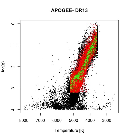
(a) APOGEE stars - Data Release 13.

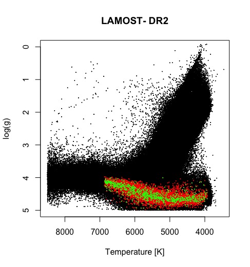
(b) LAMOST stars - Data Release 2.

Figure 1: Data selection: spectroscopic surveys used for the red giants (left) and the main sequence (right) analysis. Black points represent stars in each data release, red points are objects in the first sample selection, used to differentiate red giants stars from dwarfs and viceversa. Green points represent the 1000 stars temperature-sampling selection we have used to measure the extinction coefficient.

1 Introduction

When it comes to understanding the physics of disk galaxies, our location within the Milky Way plays an important role. By observing our visible sky and studying the astrophysical processes of its individual components, we can learn about the structure and dynamics of the Galaxy, and hence infer its formation and evolution. This prospect would not be possible only by examining other galaxies.
Accordingly, numerous spectro/photometric surveys have been conducted over the last decade, altogether spanning different spectral ranges to cover a wide variety of galactic astrophysical processes. To mention some: the Fermi Gamma-ray space Telescope (GLAST, Atwood et al. 2009) in the gamma-ray range, XMM-Newton (Mason et al. 2001, Rosen et al. 2016) in the X-ray, the Galaxy Evolution Explorer (GALEX, Martin et al. 2005) in the ultraviolet (UV), the Sloan Digital Sky Survey (SDSS, York et al. 2000) in the optical, the 2-micron All-Sky Survey (2MASS, Skrutskie et al. 2006) in the near infrared (NIR) and Planck (Planck Collaboration et al. 2011) in the far infrared-microwave range.

Yet among all, the mapping process of the Milky Way is culminating with $Gaia$, the ESA space mission that has just started providing data to study formation, dynamical, chemical and star-formation evolution (Perryman et al. 2001; Gaia Collaboration et al. 2016). Nonetheless, despite the unrivalled completeness of its information, $Gaia$, like the other surveys, does not rule out astrophysical selection effects such as the interstellar extinction.

Extinction is caused by the presence of dust in the line of sight and it has the main effect of dimming sources and reddening them. In particular, around 30$\%$ of light in the UV, optical and NIR is scattered and absorbed due to the interstellar medium (Draine 2003). In broad-band photometry, additionally, a major hurdle to face is the substantial degeneracy between extinction, effective temperature $T_{\mbox{{\scriptsize eff}}}$ and spectral energy distribution (SED). This degeneracy limits the accuracy by which any of the parameters can be estimated (Bailer-Jones 2010). Important to mention that extinction coefficients k_λ are a function of wavelength and get greater towards shorter wavelengths; they are defined as k_λ= $A_{\lambda}/A_{\mathrm{ref}}$ where $A_{\lambda}$ is the absolute absorption at any wavelength, expressed relative to the absolute absorption at a chosen reference wavelength $A_{\mathrm{ref}}$ (Cardelli et al. 1989).
Over recent years an increased number of studies focused on delivering more precise extinction coefficients values for various known pass-bands by using a combination of spectroscopic and photometric information retrieved from the most advanced surveys (e.g. Yuan et al. 2013, Schlafly et al. 2016, Xue et al. 2016).
Important to note though that in case of a wide pass-band, like the $Gaia$ one, a star which has the greater fraction of its radiation in the blue-end of the spectrum (a bluer star), has a larger extinction coefficient than a redder star. It is hence mandatory to have exact knowledge of the passband to correctly estimate the reddening factor.

Reddening of an object in a given colour can be described by the colour excess which is the difference between its observed colour and its intrinsic value. For instance the colour excess between the $Gaia$ $G$-band and the 2MASS ${K}_{\mbox{{\scriptsize S}}}$-band is given by ${\mbox{E}(G-K_{\mbox{{\scriptsize S}}})}$ = ($G-K_{\mbox{{\scriptsize S}}})_{\mathrm{obs}}-(G-K_{\mbox{{\scriptsize S}}})_{\mathrm{0}}$ where ($G-K_{\mbox{{\scriptsize S}}})_{\mathrm{obs}}$ is the observed colour and ($G-K_{\mbox{{\scriptsize S}}})_{\mathrm{0}}$ is the intrinsic one.

At the time of the publication of $Gaia$ DR1, only the nominal $Gaia\leavevmode\nobreak\ G$-passband, modelled with the most up-to-date pre-launch information, was available (Jordi et al. 2010). Recently a calibration of the $Gaia\leavevmode\nobreak\ G$-DR1 passband has been provided by Maíz Apellániz (2017). The second is redder than the first one due to some water contamination in the optics, which diminished the spectral efficiency more in the blue part of the band than in the red one (Gaia Collaboration et al. 2016). A new filter response curve will be available with the second $Gaia$ data release (DR2). Uncertainties, either in the passband determination or in the extinction law or in the stellar model atmospheres, can yield to inaccurate extinction coefficients. For these reasons and because the accurate determination of reddening to a star is key for exploiting the available $Gaia$ data, we present here a determination of $Gaia$ extinction coefficient for both red giants and dwarfs stars through a completely empirical method.
 
The manuscript is structured as follows. §2 introduces the data we used and describes the data selection for the red giants and dwarfs sample respectively. In §3 we estimate the photometric calibration relations for the main sequence. §4 describes the estimation of the theoretical extinction coefficients used in our analysis. In §5 we present the technique we used to estimate $Gaia$ $G$-band extinction coefficient (k_G) for the red giants sample, the dwarfs sample and, finally, for the union of both samples. In §6 we present the results and discuss them. Finally, §7 presents our conclusions.

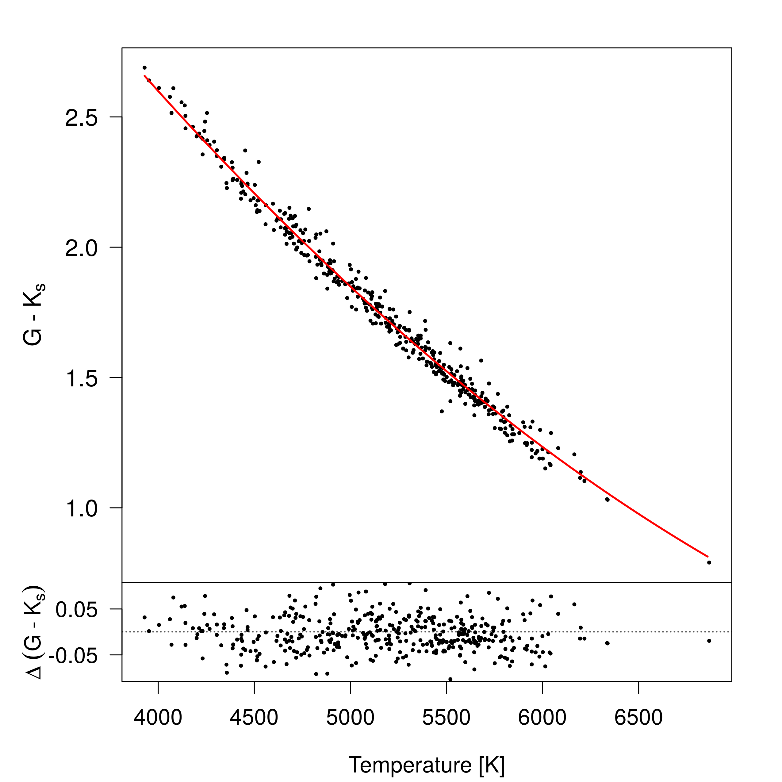
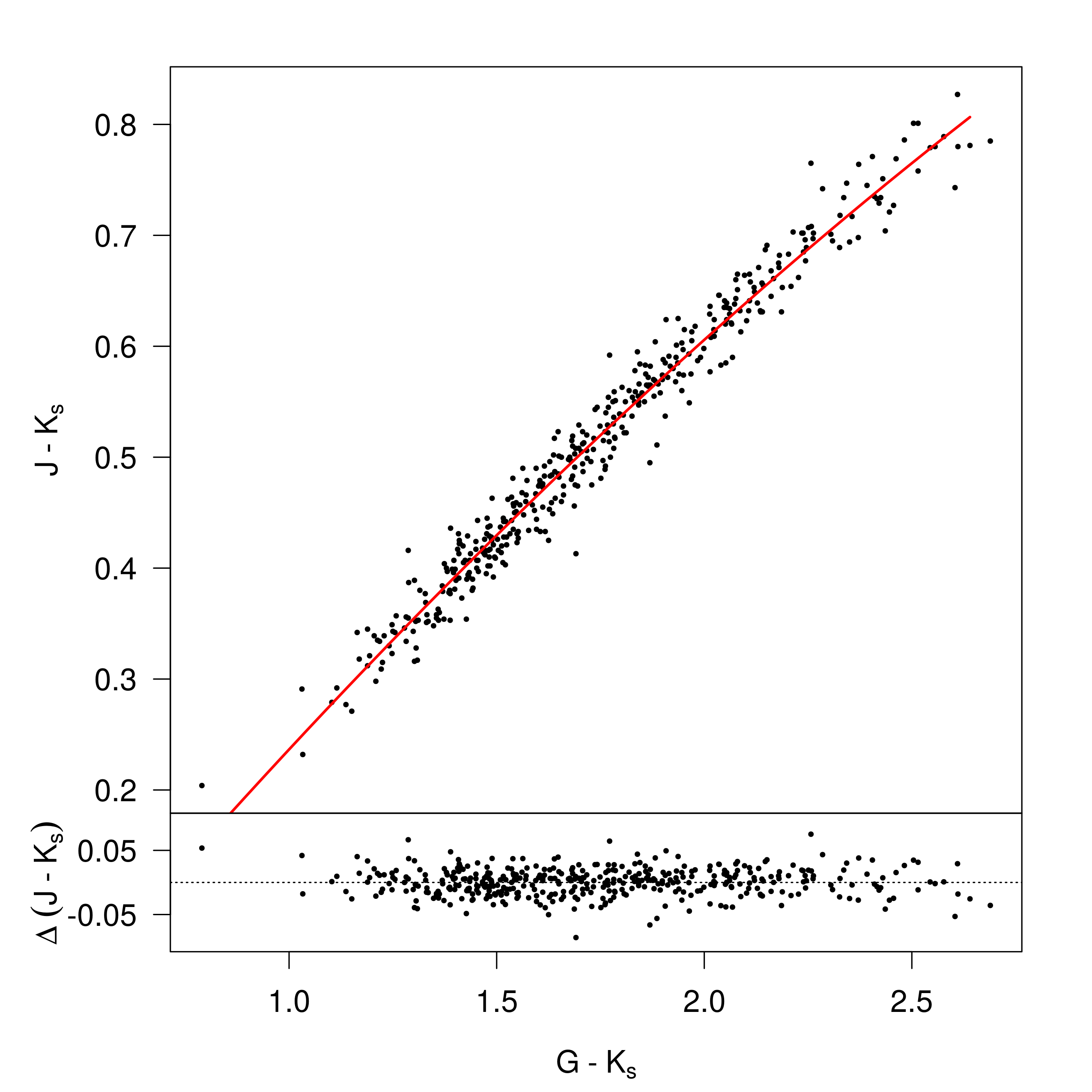
Figure 2: Main sequence photometric calibration relations: ($G-K_{\mbox{{\scriptsize S}}})_{0}$ as a function of $T_{\mbox{{\scriptsize eff}}}$ (left); ($J-K_{\mbox{{\scriptsize S}}})_{0}$ as a function of ($G-K_{\mbox{{\scriptsize S}}})_{0}$, (right). Top panels: stars (black dots) in the sample where solid red lines correspond to our calibration at solar metallicity (Eq. 1). Bottom panels: residuals (black dots) corresponding to the top panel calibration.

2 Data

For our analysis we cross-matched photometric and spectroscopic data from different surveys. More specifically for the photometric information we used the $Gaia$ DR1 and 2MASS catalogues. The 2MASS $J$, $H$, ${K}_{\mbox{{\scriptsize S}}}$ magnitudes are available for a large fraction of the $Gaia$ sources and the near-infrared extinction law is fairly well characterized (e.g. Fitzpatrick & Massa 2009).
Spectroscopic parameters, such as effective temperature $T_{\mbox{{\scriptsize eff}}}$, surface gravity $\log(g)$ and metallicity [Fe/H], were retrieved from surveys selected $ad\leavevmode\nobreak\ hoc$ for the samples analysed. Our analysis was performed on both the red giants (RG) sample and the main sequence (MS) one (Fig. 1) separately, then on both samples combined together.

2.1 The Red Giant sample

Effective temperature $T_{\mbox{{\scriptsize eff}}}$, surface gravity $\log(g)$ and metallicity [Fe/H] were retrieved from the spectroscopic survey APO Galactic Evolution Experiment (APOGEE), DR13 (Albareti et al. 2016).
The cross-match between APOGEE and $Gaia$ was done using the 2MASS ID provided in APOGEE and the 2MASS-GDR1 cross-matched catalogue (Marrese et al. 2017), where we kept only cross-matched stars with angular distance lower than 0.3″. Hence, we selected those stars with high infrared photometric quality (i.e. 2MASS ”AAA” quality flag), radial velocity error $\sigma_{\mathrm{RV}}$ ¡ 0.1  km s^-1 to exclude binary stars, and photometric errors of $\sigma_{G}$ ¡ 0.01 mag, $\sigma_{J}$ ¡ 0.03 mag and $\sigma_{{K}_{\mbox{{\scriptsize S}}}}$ ¡ 0.03 mag. The $G$-band photometric error has been later increased of 0.01 mag in quadrature to mitigate the impact of bright stars residual systematics (Evans et al. 2017, Arenou et al. 2017). Then we retained the red giants stars by screening those with colour ($G-K_{\mbox{{\scriptsize S}}})_{\mathrm{obs}}$ ¿ 1.6 mag. For stars with parallax information in $Gaia$ DR1 (TGAS), we used the same criteria as Ruiz-Dern et al. (2017):

$$\begin{array}[]{cc}G+5+5\leavevmode\nobreak\ \mbox{log}_{10}\left(\frac{\varpi+2.32\sigma_{\varpi}}{1000}\right)<4\end{array}$$

where the factor 2.32 on the parallax error $\sigma_{\varpi}$ corresponds to the 99th percentile of the parallax probability density function. When no parallax information was available, the selection was performed by filtering on the surface gravity ($\log(g)$ ¡ 3.2 dex).
Finally, we selected those stars with effective temperature 3603 K ¡ $T_{\mbox{{\scriptsize eff}}}\pm\sigma_{\mathrm{Teff}}$ ¡ 5207 K and metallicity -1.5 dex ¡ [Fe/H] ¡ 0.4 dex. to work within the same limits set for the $T_{\mbox{{\scriptsize eff}}}$ vs ($G-K_{\mbox{{\scriptsize S}}})_{\mathrm{0}}$ calibration by Ruiz-Dern et al. (2017). The application of these criteria delivered a sample of 71290 stars.

PHOTOMETRIC CALIBRATION COEFFICIENTS
	RMS	$c_{1}$	$c_{2}$	$c_{3}$	$c_{4}$	$c_{5}$	$c_{6}$
RG	0.05	13.554 $\pm$ 0.478	-20.429$\pm$1.020	8.719$\pm$0.545	0.143$\pm$0.013	-0.0002$\pm$0.009	–
MS	0.04	6.946$\pm$0.181	-6.835$\pm$0.354	1.711$\pm$0.172	–	–	–
		$c_{7}$	$c_{8}$	$c_{9}$	$c_{10}$	$c_{11}$	c12
RG	0.02	-0.227$\pm$ 0.024	0.466$\pm$0.021	-0.023$\pm$0.005	-0.016$\pm$0.002	-0.005$\pm$0.001	–
MS	0.02	-0.200$\pm$0.034	0.471$\pm$0.038	-0.03$\pm$0.01	–	–	–

Table 1: Coefficients of the calibration relations (Eq. 1) and their uncertainties for the RG sample (Ruiz-Dern et al. 2017) and MS sample (this work). The RMS corresponds to one standard deviation of the relations residuals.

2.2 The main sequence sample

For the dwarfs sample we cross-matched our photometric samples with the Large sky Area Multi-Object fiber Spectroscopic Telescope survey (LAMOST, Zhao et al. 2012) DR2, from which we retrieved effective temperature $T_{\mbox{{\scriptsize eff}}}$, surface gravity $\log(g)$ and metallicity [Fe/H]. The cross-match with 2MASS and $Gaia$ DR1 was done with a radius of 0.2″. We selected a sub-sample of objects with radial velocity error $\sigma_{\mathrm{RV}}$ ¡ 20  km s^-1 to exclude binary stars, photometric errors $\sigma_{\mathrm{G}}$, $\sigma_{\mathrm{K_{S}}}$, $\sigma_{\mathrm{J}}$ ¡ 0.03 mag and relative temperature error smaller than 5$\%$. As explained in §2.1, we increased $\sigma_{\mathrm{G}}$ of 0.01 mag in quadrature. Following we retained the main sequence stars by applying both colour and surface gravity cuts:

• $\log(g)$ -2$\sigma_{\log(g)}$ ¿ 3.5 dex

where $\sigma_{\log(g)}$ is the surface gravity error.
We set the metallicity range for the MS calibration (and consequently for the extinction coefficient estimation) to be solar-like ( -0.05 dex ¡ [Fe/H] ¡ 0.05 dex) because of the significant correlation between metallicity and effective temperature in the LAMOST data which did not allow a good convergence of the photometric calibration (see §3).

We further selected stars with temperature within the calibration temperature interval (3928 K ¡ $T_{\mbox{{\scriptsize eff}}}\pm\sigma_{\mathrm{Teff}}$ ¡ 6866 K), leaving a final sample of 17468 dwarfs.

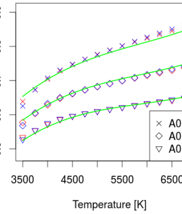
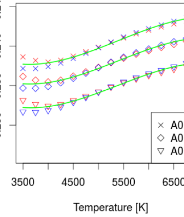
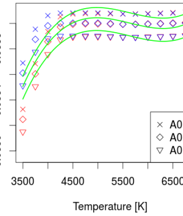
Figure 3: Theoretical extinction coefficients in the $G$- ($Gaia$), $J$- and ${K}_{\mbox{{\scriptsize S}}}$ (2MASS) bands as a function of temperature for different extinctions ($A_{0}$ = 1, 5, 10 mag) and different surface gravities: $\log(g)$ = 2.5 dex (red) and $\log(g)$ = 4 dex (blue). Green lines represent the global fit for the three absorption values.

3 Photometric Calibration

In order to empirically measure the $Gaia$ $G$-band extinction coefficient k_G, the colour excess ${\mbox{E}(G-K_{\mbox{{\scriptsize S}}})}$ and ${\mbox{E}(J-K_{\mbox{{\scriptsize S}}})}$ for our samples need to be determined. To do so we used for the RG sample the photometric calibration relations presented in Ruiz-Dern et al. (2017) while, for the MS sample, we applied the method described therein to empirically retrieve the photometric calibration relations. Specifically, the calibration relations for both samples were modelled as the following:

$$\begin{array}[]{ccl}(G-K_{\mbox{{\scriptsize S}}})_{\mathrm{0}}&=&c_{1}+c_{2}\leavevmode\nobreak\ \hat{T}+c_{3}\leavevmode\nobreak\ \hat{T}^{2}+c_{4}\leavevmode\nobreak\ \textrm{[Fe/H]}+...\\ &&+c_{5}\leavevmode\nobreak\ \textrm{[Fe/H]}^{2}+\leavevmode\nobreak\ c_{6}\leavevmode\nobreak\ \hat{T}\leavevmode\nobreak\ \textrm{[Fe/H]}^{2}\\ (J-K_{\mbox{{\scriptsize S}}})_{\mathrm{0}}&=&c_{7}+c_{8}\leavevmode\nobreak\ (G-K_{\mbox{{\scriptsize S}}})_{\mathrm{0}}+c_{9}\leavevmode\nobreak\ (G-K_{\mbox{{\scriptsize S}}})_{\mathrm{0}}^{2}\leavevmode\nobreak\ +...\\ &&+\leavevmode\nobreak\ c_{10}\leavevmode\nobreak\ \textrm{[Fe/H]}+c_{11}\leavevmode\nobreak\ \textrm{[Fe/H]}^{2}\leavevmode\nobreak\ +\leavevmode\nobreak\ ...\\ &&c_{12}\leavevmode\nobreak\ (G-K_{\mbox{{\scriptsize S}}})_{\mathrm{0}}\leavevmode\nobreak\ \textrm{[Fe/H]}\nobreak\leavevmode\end{array}$$ (1)

where $\hat{T}=T_{\mbox{{\scriptsize eff}}}$/5040 is the normalised temperature and $c_{i}$ are the coefficients reported in Table 1 for both RG and MS samples.

For calibrating the main sequence relations we selected from the sample of §2.2 only low extinction stars (E($B-V$) $<$ 0.01) selected from the recent 3D local extinction map of Capitanio et al. (2017) or the 2D map of Schlegel et al. (1998) when no distance information was available. We required the relative temperature error to be smaller than 2$\%$. The application of these further criteria left a total of 415 stars that we used for the calibration process. Please refer to Ruiz-Dern et al. (2017) for more details on the calibration method. Fig. 2 shows the relations (Eq. 1, Table 1) which were established within the interval of temperature [3928 K, 6866 K].

THEORETICAL EXTINCTION COEFFICIENTS
RG + MS	$a_{1}$	$a_{2}$	$a_{3}$	$a_{4}$	$a_{5}$	$a_{6}$	$a_{7}$
k${}_{G}\leavevmode\nobreak\ (\hat{T},A_{0})$	-0.317797257	2.538901003	-1.997742387	0.572289388	-0.013179503	0.000607315	-0.01126344
k${}_{G}\leavevmode\nobreak\ (\hat{T},A_{0})$ - DR1	-0.279133556	2.373624663	-1.878795709	0.53904796	-0.011673326	0.000544945	-0.010233727
k${}_{J}\leavevmode\nobreak\ (\hat{T},A_{0})$	0.252033852	-0.042526876	0.044560182	-0.013883035	-0.000239872	8.45E-07	-1.96E-05
k${}_{{K}_{\mbox{{\scriptsize S}}}}\leavevmode\nobreak\ (\hat{T},A_{0})$	0.073839341	0.03381806	-0.03063728	0.009124118	-1.95E-05	9.66E-09	-6.81E-07
k${}_{G}\leavevmode\nobreak\ ((G-K_{\mbox{{\scriptsize S}}})_{\mathrm{0}},A_{0})$	0.935556283	-0.090722012	0.014422056	-0.002659072	-0.030029634	0.000607315	0.002713748
k${}_{J}\leavevmode\nobreak\ ((G-K_{\mbox{{\scriptsize S}}})_{\mathrm{0}},A_{0})$	0.242998063	-0.001759252	0.000107601	2.54E-05	-0.000268996	8.45E-07	4.60E-06
k${}_{{K}_{\mbox{{\scriptsize S}}}}\leavevmode\nobreak\ ((G-K_{\mbox{{\scriptsize S}}})_{\mathrm{0}},A_{0})$	0.086033161	7.65E-05	8.54E-06	-1.52E-05	-2.00E-05	-	-
k${}_{G}\leavevmode\nobreak\ ((G-K_{\mbox{{\scriptsize S}}})_{\mathrm{0}},A_{0})$ - DR1	0.882095056	-0.086780236	0.01511573	-0.002963829	-0.027054718	0.000544945	0.002604135
k${}_{J}\leavevmode\nobreak\ ((G-K_{\mbox{{\scriptsize S}}})_{\mathrm{0}},A_{0})$ - DR1	0.243062354	-0.001899476	0.000140615	2.58E-05	-0.000269124	8.45E-07	4.86E-06
k${}_{{K}_{\mbox{{\scriptsize S}}}}\leavevmode\nobreak\ ((G-K_{\mbox{{\scriptsize S}}})_{\mathrm{0}},A_{0})$ - DR1	0.086025432	9.23E-05	3.32E-06	-1.65E-05	-2.00E-05	-	-

Table 2: Theoretical extinction coefficients for the $Gaia\leavevmode\nobreak\ G$-band, both pre-launch (Jordi et al. 2010) and G-DR1 (Maíz Apellániz 2017) passbands, and for $J$- and ${K}_{\mbox{{\scriptsize S}}}$-bands, measured by using the Fitzpatrick & Massa (2007) extinction law and the Kurucz Spectral Energy Distributions from Castelli & Kurucz (2003) (see §4). The extinction coefficients are modelled as function of ($\hat{T},A_{0}$) and ($(G-K_{\mbox{{\scriptsize S}}})_{\mathrm{0}},A_{0}$), Eq. (3), and they are valid for both the red giants and the main sequence samples for 3500 K$<T_{\mbox{{\scriptsize eff}}}<$7000 K and $A_{0}$ ¡ 20 mag

4 Theoretical extinction coefficients

We computed the theoretical extinction coefficients k_m using the Fitzpatrick & Massa (2007) extinction law $E_{\lambda}$, the Kurucz Spectral Energy Distributions $F_{\lambda}$ from Castelli & Kurucz (2003) and the filters transmissions $T_{\lambda}$ :

$$k_{m}A_{0}=A_{m}=m-m_{0}=-2.5\log_{10}\left(\frac{\int F_{\lambda}T_{\lambda}E_{\lambda}^{A_{0}}d\lambda}{\int F_{\lambda}T_{\lambda}d\lambda}\right)$$ (2)

with $A_{0}$ the interstellar extinction at $\mathrm{\lambda}$ = 550 nm ($Gaia$ reference value). While the Fitzpatrick & Massa (2007) extinction law was derived using hot stars, this extinction law was calibrated using the full star spectral energy distribution and therefore should be also valid for the lower temperature stars of our sample.

For 2MASS transmissions were taken from Cohen et al. (2003). For comparison purposes we used the $Gaia$ pre-launch transmission and the Gaia G-DR1 transmission of Maíz Apellániz (2017).

As shown by Jordi et al. (2010), in such a large band as $Gaia$ $G$-band ($\sim$330 - 1050 nm), the extinction coefficient varies strongly with temperature and the extinction itself, but less with surface gravity and metallicity. We therefore modelled the extinction coefficients as a function of $A_{0}$ and $T_{\mbox{{\scriptsize eff}}}$, following the formula:

$$\mbox{k}_{m}=a_{1}+a_{2}\mbox{ X}+a_{3}\mbox{ X}^{2}+a_{4}\mbox{X}^{3}+a_{5}A_{0}+a_{6}A_{0}^{2}+a_{7}\mbox{X}A_{0}$$ (3)

where X is either $\hat{T}=T_{\mbox{{\scriptsize eff}}}$/5040 or ($G-K_{\mbox{{\scriptsize S}}})_{\mathrm{0}}$, depending if we are analysing the extinction coefficient as a function of the normalised temperature or the colour, respectively. The parameters $a_{i}$ are the coefficients of the fit in each photometric band $m$.

Table 2 reports the coefficients $a_{i}$ for the theoretical estimation of the global k_J and k${}_{{K}_{\mbox{{\scriptsize S}}}}$ coefficients valid for both red giants and main sequence stars, as well as k_G, which was computed by using the $Gaia$ pre-launch modelled filter response.

The fit is performed using extinctions computed on a grid with a spacing of 250 K in $T_{\mbox{{\scriptsize eff}}}$ and 0.01 mag in $A_{0}$ with 0.01 mag $<\mathrm{A}_{0}<20$ mag and 3500 K $<T_{\mbox{{\scriptsize eff}}}<7000$ K and two surfaces gravities: $\log(g)$ = 2.5 dex and 4 dex. The result is shown in Fig. 3. We checked that high order parameters in the polynomials are needed with an ANOVA test. Only for the ${K}_{\mbox{{\scriptsize S}}}$-band and for relatively low extinctions ($A_{0}<5$ mag) coefficients $a_{5}$ and $a_{6}$ are not significant. In particular residuals of the fit are smaller than 0.3% for k${}_{{K}_{\mbox{{\scriptsize S}}}}$, 0.2% for k_J and 4.5% for k_G. For k_G residuals decrease to 2.4% when the fit is performed just for $A_{0}<5$ mag. For comparison, we have estimated the extinction coefficients using the Cardelli et al. (1989) extinction law, and compared them to the ones obtained with the Fitzpatrick & Massa (2007) law: the difference is of 37% in the ${K}_{\mbox{{\scriptsize S}}}$-band, 20% in the $J$-band and 5% in the nominal $G$-band. Jordi et al. (2010) also assessed that $R_{V}$ variation does not have a significant impact on k_G. On the other hand, the ${K}_{\mbox{{\scriptsize S}}}$- and $J$-bands are much less sensitive to spectral type variations (Fig. 3): for instance the difference between a red giant star and Vega is of only 0.07% for the ${K}_{\mbox{{\scriptsize S}}}$-band, 1% for the $J$-band, while it is of 21% in the $G$-band.

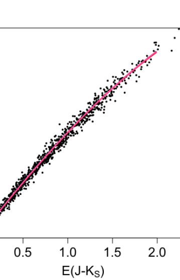
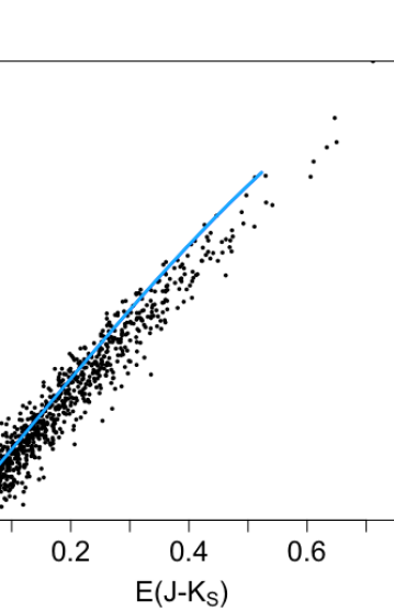
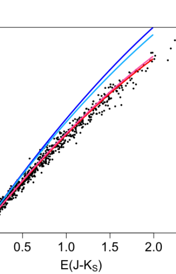
Figure 4: Colour excesses E$(G-K_{\mbox{{\scriptsize S}}})$ versus E$(J-K_{\mbox{{\scriptsize S}}})$ for the red giants sample (left), the main sequence sample (centre) and the combined sample (right). Black dots are the 1000 stars selected in each sample. Solid lines represent the colour excess increase with extinction for a reference temperature $T_{\mbox{{\scriptsize eff}}}$ (4136 K for RG, red; 5550 K for MS, dark blue) and the corresponding reference colour $(G-K_{\mbox{{\scriptsize S}}})_{0}$ (2.49 for RG, pink; 1.49 for MS, light blue). Note that some lines may overlap. Their cut corresponds to the interval of absorption $A_{0}$ indicated in Table 3 (13.3 for RG, 3.5 for MS).

5 Method

To empirically measure the $G$-band extinction coefficient as a function of either temperature or colour ($G-K_{\mbox{{\scriptsize S}}})_{\mathrm{0}}$ we implemented a Markov-Chain Monte Carlo method (MCMC, Brooks et al. 2011) to sample the parameter space and to properly account for errors. The MCMC used the jags algorithm (Plummer 2003) encompassed in runjags library, for R programme language.

In order to not affect the MCMC convergence by having an un-even distribution in extinction and temperature, we used a two dimensional kernel density estimation of the ${\mbox{E}(G-K_{\mbox{{\scriptsize S}}})}$ vs $T_{\mbox{{\scriptsize eff}}}$ stellar probability space to select a more uniform sub-sample of 1000 stars for each RG and MS (Fig. 1) and combined (RG+MS) sample. The number of stars in each sub-sample (i.e. 1000) is optimised to be statistically relevant for the analysis yet without having a large disproportion of elements between bins (which could cause the analysis to be biased towards the most populated bin).

Intrinsic colours ($G-K_{\mbox{{\scriptsize S}}})_{\mathrm{0}}$ and $(J-K_{\mbox{{\scriptsize S}}})_{\mathrm{0}}$ were taken from Eq. (1) where temperature and metallicity were set to be $T^{\prime}_{\mbox{{\scriptsize eff}}}\sim\mathcal{N}(T_{\mbox{{\scriptsize eff}}},\sigma_{\mathrm{T_{\mbox{{\scriptsize eff}}}}}^{2})$ and $\textrm{[Fe/H]}^{\prime}\sim\mathcal{N}($[Fe/H]$,\sigma_{\mathrm{\textrm{[Fe/H]}}}^{2})$ where $\mathcal{N}$ is the normal distribution and $\sigma_{\mathrm{Teff}}^{2}$, $\sigma_{\mathrm{\textrm{[Fe/H]}}}^{2}$ the respective observed variances.

Observed colours ($G-K_{\mbox{{\scriptsize S}}})_{\mathrm{obs}}$ and ($J-K_{\mbox{{\scriptsize S}}})_{\mathrm{obs}}$ were set to be

$$\begin{array}[]{ccl}(G-K_{\mbox{{\scriptsize S}}})_{\mathrm{obs}}&\sim&\mathcal{N}((G-K_{\mbox{{\scriptsize S}}})_{\mathrm{0}}+(\mathrm{k}_{G}-\mathrm{k}_{{K}_{\mbox{{\scriptsize S}}}})\cdot A_{0}^{\prime},\leavevmode\nobreak\ \sigma^{2}_{G-{K}_{\mbox{{\scriptsize S}}}})\\ (J-K_{\mbox{{\scriptsize S}}})_{\mathrm{obs}}&\sim&\mathcal{N}((J-K_{\mbox{{\scriptsize S}}})_{\mathrm{0}}+(\mathrm{k}_{J}-\mathrm{k}_{{K}_{\mbox{{\scriptsize S}}}})\cdot A_{0}^{\prime},\leavevmode\nobreak\ \sigma^{2}_{J-{K}_{\mbox{{\scriptsize S}}}})\end{array}$$ (4)

where $\sigma^{2}_{G-{K}_{\mbox{{\scriptsize S}}}}=(\sigma_{G}^{2}+\sigma_{{K}_{\mbox{{\scriptsize S}}}}^{2}$) and $\sigma^{2}_{J-K_{\mbox{{\scriptsize S}}}}=(\sigma_{J}^{2}+\sigma_{{K}_{\mbox{{\scriptsize S}}}}^{2}$) and where $\sigma_{G},\sigma_{J},\sigma_{{K}_{\mbox{{\scriptsize S}}}}$ are the photometric errors. k_J and k${}_{{K}_{\mbox{{\scriptsize S}}}}$ are the extinction coefficients for $J$- and ${K}_{\mbox{{\scriptsize S}}}$-bands as function of either $\hat{T}$ or colour. All along our analysis k_J and k${}_{{K}_{\mbox{{\scriptsize S}}}}$ are fixed to the theoretical values (see §4).
For each star in the sample we used its colour excess ${\mbox{E}(J-K_{\mbox{{\scriptsize S}}})}$ and initial extinction coefficients values (computed at $A_{0}$ = 0 mag), to get an initial value of the absorption $A_{0}$, which we then set in the MCMC as mean of a truncated normal distribution $A_{0}^{\prime}\sim$ $\mathcal{N}(A_{0}$, 0.2) lying within the positive interval $A_{0}^{\prime}$ > 0. For a given star, its initial $A_{0}$ value does not change within the MCMC. Finally we set the coefficients $a_{i}$ of Eq. (3) free to vary following the uninformative prior distribution $a_{i}\sim\mathcal{N}$(0, 1000).

Each MCMC was run using two chains with $10^{4}$ steps and a burn-in of 4000. We used standardised variables to improve the efficiency of MCMC sampling (hence reducing the autocorrelation in the chains) and checked for chain convergence by using the Gelman-Rubin convergence diagnostic. We tested the significance of coefficients $a_{i}$ through the Deviance Information Criterion (DIC), a model fit measure that penalises model complexity.

We produced 10 different sub-samples of 1000 stars (uniform in $T_{\mbox{{\scriptsize eff}}}$ and ${\mbox{E}(G-K_{\mbox{{\scriptsize S}}})}$), each of which was processed through an MCMC. The mean of those runs is reported in Table 3.

We run this analysis for the red giants first, then for the main sequence stars, and finally for both samples combined in a single one.

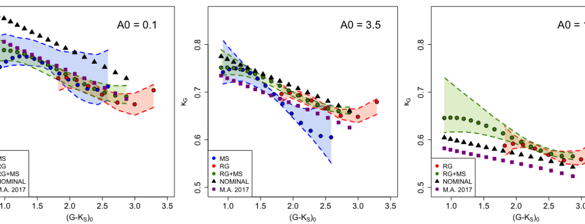
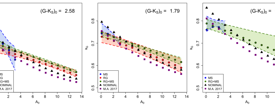
Figure 5: Direct comparison of the empirical extinction coefficient k_G as a function of ($G-K_{\mbox{{\scriptsize S}}})_{0}$ for $A_{0}$ = 0.1, 3.5, 13.3 mag (top panel) and $A_{0}$ for ($G-K_{\mbox{{\scriptsize S}}})_{0}$ = 2.58, 1.79, 0.98 (bottom panel, which corresponds to $T_{\mbox{{\scriptsize eff}}}$ = 4020, 5080, 6500 K). $A_{0}$ = 3.5, 13.3 mag are the limit values for the MS and RG samples respectively (see Table 3) while ($G-K_{\mbox{{\scriptsize S}}})_{0}$ = 2.58, 1.79 are the maximal colour of LAMOST and the minimal colour of APOGEE, respectively. ($G-K_{\mbox{{\scriptsize S}}})_{0}$ = 0.98 is a sample case to show the behaviour at low colour indexes (i.e. high temperatures). Dots show the k_G mean value while the shaded area show the 95$\%$ interval of confidence (see §5.1). Colours correspond to the red giants (RG, red), the main sequence (MS, blue) and unified sample (RG+MS, green). Black triangles and magenta squares show the theoretical k_G coefficient computed with the Gaia pre-launch (NOMINAL, Jordi et al. 2010) and Gaia $G$-DR1 (M.A. 2017, Maíz Apellániz 2017) passbands, respectively.

5.1 Error analysis

To derive our confidence interval, we use the bootstrap resampling technique (Efron 1987). The bootstrap resampling consists of generating a large number of data sets, each with an equal amount of points randomly drawn with replacement from the original sample. It allows us to take into account not only measurement errors but also sampling-induced errors, which are here a relevant factor due to the uneven distribution of stars in temperature and colour excess space.
Bootstrapped $a_{i}$ errors are larger than MCMC chains errors by an average factor of 5, 3 and 7 for $T_{\mbox{{\scriptsize eff}}}$ case and 16, 3 and 4 for the ($G-K_{\mbox{{\scriptsize S}}})_{0}$ case for RG, MS and RG+MS, respectively. Important to note though that these uncertainties are constrained by the precision of the data used, more specifically by the error on the temperature, whose median is $\tilde{\sigma}_{\mathrm{Teff}}\sim$ 69 K for APOGEE data and $\tilde{\sigma}_{\mathrm{Teff}}\sim$ 115 K for LAMOST data.

We carried out the MCMC runs on 100 bootstrapped samples and derived the confidence levels through the percentile method, which we report in Table 3 and Fig. 5.

EMPIRICAL kG VALUES
RG	$T_{\mbox{{\scriptsize eff}}}$ int.	$A_{0}$	$a_{1}$	$a_{2}$	$a_{3}$	$a_{4}$	$a_{5}$	$a_{6}$	$a_{7}$
k${}_{G}\leavevmode\nobreak\ [\hat{T},A_{0}]$	[3680, 5080]	¡ 13.3	15.25	-51.059	59.12	-22.57	2.41E-03	-1.42E-04	-1.19E-02
$\sigma_{kG}\leavevmode\nobreak\ [\hat{T},A_{0}]$			3.69	13.052	15.29	5.94	4.73E-03	9.01E-05	5.01E-03
	$(G-K_{\mbox{{\scriptsize S}}})_{\mathrm{0}}$ int.	$A_{0}$	$a_{1}$	$a_{2}$	$a_{3}$	$a_{4}$	$a_{5}$	$a_{6}$	$a_{7}$
k${}_{G}\leavevmode\nobreak\ [(G-K_{\mbox{{\scriptsize S}}})_{\mathrm{0}},A_{0}]$	[1.82, 2.87]	¡ 13.3	-0.72	1.94	-0.84	0.116	-1.24E-02	-1.07E-04	1.68E-03
$\sigma_{kG}\leavevmode\nobreak\ [(G-K_{\mbox{{\scriptsize S}}})_{\mathrm{0}},A_{0}]$			0.93	1.13	0.45	0.059	2.83E-03	1.23E-04	1.14E-03
MS	$T_{\mbox{{\scriptsize eff}}}$ int.	$A_{0}$	$a_{1}$	$a_{2}$	$a_{3}$	$a_{4}$	$a_{5}$	$a_{6}$	$a_{7}$
k${}_{G}\leavevmode\nobreak\ [\hat{T},A_{0}]$	[4020, 6620]	¡ 3.5	4.40	-11.405	11.52	-3.77	-0.051	-6.60E-03	0.056
$\sigma_{kG}\leavevmode\nobreak\ [\hat{T},A_{0}]$			1.38	4.028	3.85	1.21	0.044	1.65E-03	0.038
	$(G-K_{\mbox{{\scriptsize S}}})_{\mathrm{0}}$ int.	$A_{0}$	$a_{1}$	$a_{2}$	$a_{3}$	$a_{4}$	$a_{5}$	$a_{6}$	$a_{7}$
k${}_{G}\leavevmode\nobreak\ [(G-K_{\mbox{{\scriptsize S}}})_{\mathrm{0}},A_{0}]$	[0.92, 2.59]	¡ 3.5	0.32	0.88	-0.53	0.097	0.038	-7.06E-03	-0.017
$\sigma_{kG}\leavevmode\nobreak\ [(G-K_{\mbox{{\scriptsize S}}})_{\mathrm{0}},A_{0}]$			0.15	0.30	0.19	0.036	0.020	1.72E-03	0.013
RG + MS	$T_{\mbox{{\scriptsize eff}}}$ int.	$A_{0}$	$a_{1}$	$a_{2}$	$a_{3}$	$a_{4}$	$a_{5}$	$a_{6}$	$a_{7}$
k${}_{G}\leavevmode\nobreak\ [\hat{T},A_{0}]$	[3680, 6620]	¡ 13.3	3.24	-8.31	8.72	-2.92	-7.55E-03	-8.35E-05	-6.73E-04
$\sigma_{kG}\leavevmode\nobreak\ [\hat{T},A_{0}]$			0.55	1.67	1.67	0.55	6.24E-03	1.19E-04	6.73E-03
	$(G-K_{\mbox{{\scriptsize S}}})_{\mathrm{0}}$ int.	$A_{0}$	$a_{1}$	$a_{2}$	$a_{3}$	$a_{4}$	$a_{5}$	$a_{6}$	$a_{7}$
k${}_{G}\leavevmode\nobreak\ [(G-K_{\mbox{{\scriptsize S}}})_{\mathrm{0}},A_{0}]$	[0.92, 2.87]	¡ 13.3	0.697	0.219	-0.154	2.69E-02	-1.14E-02	-6.84E-07	6.58E-04
$\sigma_{kG}\leavevmode\nobreak\ [(G-K_{\mbox{{\scriptsize S}}})_{\mathrm{0}},A_{0}]$			0.059	0.083	0.037	5.51E-03	3.43E-03	1.38E-04	1.30E-03

Table 3: Empirical extinction coefficient k_G for the $Gaia$ $G$-band as a function of absorption $A_{0}$ and the normalised temperature $\hat{T}$ or colour $(G-K_{\mbox{{\scriptsize S}}})_{\mathrm{0}}$ for the red giants sample (RG), the main sequence sample (MS) and both samples combined in only one (RG + MS). For each sample we report temperature, colour and extinction intervals of validity. The errors (1$\sigma$ uncertainties) on the coefficients have been measured with the bootstrap technique.

6 Results and Discussion

All MCMCs to estimate both k${}_{G}[\hat{T},A_{0}$] and k${}_{G}[(G-K_{\mbox{{\scriptsize S}}})_{0},A_{0}$] were found to converge for all the three samples analysed (RG, MS and RG+MS).

Table 3 reports final $a_{i}$ coefficients and their uncertainties, as well as k_G intervals of validity (i.e. temperature, colour and extinction). The temperature interval (and consequently the colour one) is the range common to all the bootstrapped samples employed in our analysis. The maximum extinction ($A_{0}$) depends on the ${\mbox{E}(J-K_{\mbox{{\scriptsize S}}})}$ data distribution. For conservative reasons, as the colour excess distribution for the three samples is right-skewed (i.e. small number of stars with large colour excess), we set the $A_{0}$ upper limit by cutting ad hoc the tail of each distribution after a visual inspection, i.e. where we had small gap in the data or where the stars were too few for giving a robust solution.

We note that, while we tested the significance of high order $a_{i}$ parameters with the DIC test (see §5), some coefficients in Table 3 appear as non-significant due to bootstrap errors being significantly larger than the MCMC derived ones.

We show in Fig. 4 the retrieved empirical colour excess E$(G-K_{\mbox{{\scriptsize S}}})$ versus E($J-K_{\mbox{{\scriptsize S}}})$ for the three samples. We picked the median of the high-extinction stars’ temperature as reference temperature. For the MS sample, the median temperature does not change significantly for high-extinction stars while for the RG the high-extinction stars are the coolest as they are intrinsically significantly brighter.
The three stellar samples delivered consistent results. We display in Fig. 5 the direct comparison of k_G as a function of both colour and extinction. The ”wavy” aspect of the top panel is a direct consequence of the third order polynomial used for the modelling, where the need of the high order had been tested by an ANOVA (see §4). The polynomial is well behaved in the interior of the fitting regime, but at the edges it generates a phenomenon termed “polynomial wiggle”, whose main consequence is the lack-of-accuracy given by the large oscillations of the polynomial at both ends. For this reason the accuracy is lower at the borders of the temperature and extinction $A_{0}$ intervals of validity (Fig. 5). For the extinction the effect is less prominent as the polynomial is only of degree two in $A_{0}$. However, its impact is seen in Fig. 5 (top panel, plot 2) where the k_G are not consistent with RG or RG+MS due to this polynomial edge effect and lack of high extinction stars in the MS sample.
While there is a small difference between the empirically retrieved and the theoretical extinction coefficient (both nominal and G-DR1 (Maíz Apellániz 2017) passbands), the amplitude and the trend of the variation as a function of temperature (or colour) and extinction is similar. Our empirical coefficients are, as expected, closer to the G-DR1 passband than the nominal passband in the low extinction regime. However they are larger than the theoretical ones for $A_{0}$>3 mag for the nominal passband, and $A_{0}\gtrsim$ 2 mag for the G-DR1 passband. With the information currently in our possession we are not able to address this issue, which may be due to uncertainties in the extinction law or in the filter response determination, we will though perform the same study for the coming $Gaia$ DR2 release in order to determine the DR2 k_G extinction coefficients and to clarify this problem.

We overall recommend the use of the combined sample (RG+MS) coefficients using the intrinsic colour ($G-K_{\mbox{{\scriptsize S}}})_{0}$. The use of the combined sample gives an unique solution for both stellar evolution stages which it is less affected by the polynomial wiggle effect. The colour is also less affected by the temperature scale difference between LAMOST and APOGEE.

7 Conclusions

We present here the empirical estimation of the $Gaia$ $G$-band extinction coefficient k_G that can be used as unique solution for both red giants and main sequence stars.

We used high quality photometry in the $Gaia\leavevmode\nobreak\ G$-DR1 and 2MASS $J$- and ${K}_{\mbox{{\scriptsize S}}}$-bands combined with the APOGEE DR13 and the LAMOST DR2 spectroscopic surveys to retrieve effective temperatures for red giants and dwarfs samples respectively. We implemented a Markov Chain Monte Carlo (MCMC) method where we used the photometric calibration $T_{\mbox{{\scriptsize eff}}}$ vs $(G-K_{\mbox{{\scriptsize S}}})_{\mathrm{0}}$ and $(J-K_{\mbox{{\scriptsize S}}})_{\mathrm{0}}$ vs $(G-K_{\mbox{{\scriptsize S}}})_{\mathrm{0}}$ relations (method presented by Ruiz-Dern et al. 2017), to estimate the extinction coefficient k_G as a function of the normalised temperature $\hat{T}$ = $T_{\mbox{{\scriptsize eff}}}$/5040 or colour $(G-K_{\mbox{{\scriptsize S}}})_{\mathrm{0}}$ and absorption $A_{0}$.

We compared each empirical k_G coefficient (measured for the dwarfs, the red giants and the combined sample) first with the theoretical one (estimated using both the $Gaia$ $G$-passband modelled pre-launch and the $G$-DR1 (Maíz Apellániz 2017) passband), then between themselves. For the first case, while we find a small difference between our results and the theoretical extinction coefficients for large extinctions, we confirmed that both theoretical and empirical k_G have the same trend. For the second case we find consistent results.

We modelled the extinction coefficient as a function of both stellar temperature (or intrinsic colour) and absorption to more precisely account for the degeneracy between extinction and spectral energy distribution. We believe that this approach is the best practice, particularly for large passbands such as the $Gaia\leavevmode\nobreak\ G$-band, where the extinction coefficient varies strongly within the band itself.

The results presented here are valid for the $Gaia$ $G$-DR1 band data and they are constrained by the precision of the spectrometric data used for our analysis. The same study will be performed for the $Gaia$ DR2 release (April 2018) with the inclusion of the estimation of the extinction coefficient valid for both BP and RP bands.