A distinguishable single excited-impurity in a Bose-Einstein condensate

Abstract

We investigate the properties of a distinguishable single excited state impurity pinned in the center of a trapped Bose-Einstein condensate (BEC) in a one-dimensional harmonic trapping potential by changing the bare mass of the impurity and its interspecies interaction strength with the BEC. We model our system by using two coupled differential equations for the condensate and the single excited-impurity wave function, which we solve numerically. For equilibrium, we obtain that an excited-impurity induces two bumps or dips on the condensate for the attractive- or repulsive-interspecies coupling strengths, respectively. Afterwards, we show that the excited-impurity induced imprint upon the condensate wave function remains present during a time-of-flight (TOF) expansion after having switched off the harmonic confinement. We also investigate shock-waves or gray-solitons by switching off the interspecies coupling strength in the presence of harmonic trapping potential. During this process, we found out that the generation of gray bi-soliton or gray quad-solitons (four-solitons) depends on the bare mass of the excited-impurity in a harmonic trap.

I Introduction

Certainly, the physics of trapped condensates has emerged as one of the most exciting fields of physics in last few decades. During last few years, substantial experimental and theoretical progress has been made in the study of the properties of this new state of matter. The remarkable experimental realization of a Bose-Einstein condensate mixture composed of two spin states of ${}^{87}\text{Rb}$ Andrews et al. (1997); Myatt et al. (1997) has a rapid compelling interest in the physics of a new class of quantum fluids: the two or more species Bose-Einstein condensates Hall et al. (1998); Kohler and Sols (2002); Papp et al. (2008); McCarron et al. (2011). Multi-species condensates (MSC) offer new degrees of freedom, which give rise to a rich set of new issues Cazalilla et al. (2011); He et al. (2015), at the heart of many of these issues is the presence of interspecies interactions and the resulting coupling of the two condensates. Previous theoretical treatments have shown that due to interspecies interactions, the ground state density distribution of MSC can display novel structures that do not exist in a one-species condensate Ho and Shenoy (1996); Pu and Bigelow (1998). The investigation of a hybrid system requires progress on several different fronts. For example, from last few decades, many theoretical and experimental researchers focus on a single-particle impurity control in a many-body system for the detection and engineering of strongly correlated quantum states W. S. Bakr et al. (2009); J. F. Sherson et al. (2010); Serwane et al. (2011); Ratschbacher Lothar et al. (2012); Schurer et al. (2014, 2015).

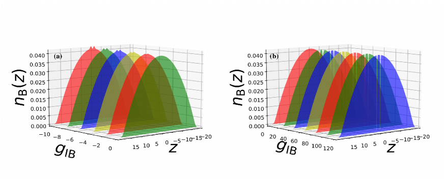
Figure 1: Numerical density profile of BEC for (a) negative and (b) positive values of $g_{\text{IB}}$ as mentioned in the figures for the experimental coupling strength value $G_{\text{B}}=4.71$ in dimensionless units.

Individually controllable impurities in a quantum gas grants access to a huge number of proposed novel applications Schirotzek et al. (2009); Palzer et al. (2009); C. Zipkes et al. (2010); Schmid et al. (2010). In the direction of quantum information processing, atomtronics applications are envisioned with single atoms acting as switches for a macroscopic system in an atomtronics circuit Micheli et al. (2004); two impurity atoms immersed in a quantum gas can be employed for a transfer of quantum information between the atoms Klein and Fleischhauer (2005), or individual qubits can be cooled preserving the internal state of coherence Daley et al. (2004); Griessner et al. (2006). Adding impurities and, hence, polarons one by one allow experimentalists to track the transition even to the many-body regime and, moreover, yield information about spatial cluster formation Klein et al. (2007); Casteels et al. (2011); Santamore and Timmermans (2011); Hohmann et al. (2015). Furthermore, adding single impurities one-by-one to an initially integrable system, such as a quasi one-dimensional Bose gas Kinoshita et al. (2006), allows one to controllably induce the thermalization of a non equilibrium quantum state. The coupling of impurities with condensed matter helps to understand material properties such as molecule formation and electrical conductivity Ng and Bose (2008); A. D. Lercher et al. (2011); Spethmann et al. (2012a, b); J. B. Balewski et al. (2013).

Recently, we investigated static and dynamical propertied of a single ground state impurity ${}^{133}\text{Cs}$ in the center of a trapped ${}^{87}\text{Rb}$ BEC Akram and Pelster (2016a). We studied the physical similarities and differences of bright shock waves and gray/dark bi-solitons, which emerge for an initial negative and positive interspecies coupling constant, respectively Akram and Pelster (2016a). In this letter, we want to extend our previous work to the single excited impurity in the center of a trapped BEC. In the following, in Sec. II, we define two coupled one-dimensional differential equations (1DDEs), where one equation is nothing but a quasi one dimensional Gross-Pitaevskii equation (1DGPE) with a potential term stemming from the excited-impurity and the second equation is a typical Schrödinger wave equation with an additional potential originating from the BEC. Afterwards, we show that the single excited state impurity (SESI) imprint upon the condensate wave function strongly depends upon whether the effective SESI-BEC coupling strength is attractive or repulsive. Subsequently, the dynamics of the SESI imprint upon the condensate wave function is discussed in detail in Sec. III. Here, we note that for an attractive interspecies coupling strength the excited-impurity imprint does not decay but decreases for a repulsive interspecies coupling strength in a time-of-flight (TOF). In the same Sec. III, we discuss the creation of shock-waves or gray quad-solitons in a harmonic trap, by switching off the attractive or repulsive Rb-Cs coupling strength. Finally, in Sec. IV we make concluding remarks and comment on the realization of the proposed model system.

II Model

We assume an effective quasi one-dimensional setting with $\omega_{\text{z}}\ll\omega_{\text{r}}$, so the theoretical model for describing the time evolution of two-component BECs is the following coupled GP equations as

$$i\hbar\frac{\partial}{\partial t}\psi(z,t)=\left\{-\frac{\hbar^{2}}{2m_{B}}\frac{\partial^{2}}{\partial z^{2}}+\frac{m_{\text{B}}\omega_{\text{z}}^{2}}{2}z^{2}+G_{\text{IB}}\lvert\psi_{\text{I}}\left(z,t\right)\lvert^{2}\right.$$

$$\left.+G_{\text{B}}\lvert\psi(z,t)\lvert^{2}\right\}\psi(z,t),$$ (1)

$$i\hbar\frac{\partial}{\partial t}\psi_{\text{I}}\left(z,t\right)=\left\{-\frac{\hbar^{2}}{2m_{\text{I}}}\frac{\partial^{2}}{\partial z^{2}}+\frac{m_{\text{I}}\omega_{\text{Iz}}^{2}}{2}z^{2}+G_{\text{BI}}\lvert\psi\left(z,t\right)\lvert^{2}\right\}$$

$$\times\psi_{\text{I}}\left(z,t\right).$$ (2)

where $\psi(z,t)$ denotes the macroscopic condensate wave function for the ${}^{87}\text{Rb}$ BEC and $\psi_{\text{I}}\left(z,t\right)$ describes ${}^{133}\text{Cs}$ single excited state impurity with $z$ being the spatial coordinate, here $m_{\text{B}}$ and $m_{\text{I}}$ stands for the mass of the ${}^{87}\text{Rb}$ and ${}^{133}\text{Cs}$ atom, respectively. In the above Eq. (1), $G_{\text{B}}=2N_{\text{B}}a_{\text{B}}\hbar\omega_{\text{r}}$ represents the one-dimensional ${}^{87}\text{Rb}$ coupling strength, where $N_{\text{B}}=200$ denotes the number of ${}^{87}\text{Rb}$ atoms, and the s-wave scattering length is $a_{\text{B}}=94.7~{}{\rm{a}_{0}}$ with the Bohr radius ${\rm{a}_{0}}$. In the first equation, $G_{\text{IB}}=N_{\text{I}}g_{\text{IB}}$ stands for the impurity-BEC coupling where $g_{\text{IB}}=2a_{\text{IB}}\hbar\omega_{\text{r}}f\left(\omega_{\text{Ir}}/\omega_{\text{r}}\right)$ and $f\left(\omega_{\text{Ir}}/\omega_{\text{r}}\right)=\left[1+\left(m_{\text{B}}/m_{\text{I}}\right)\right]/\left[1+\left(m_{\text{B}}\omega_{\text{r}}\right)/\left(m_{\text{I}}\omega_{\text{Ir}}\right)\right]$ represents a geometric function Akram and Pelster (2016a), which depends on the ratio of the trap frequencies, and $N_{\text{I}}=1$ stands for the number of excited-impurity atoms, and $a_{\text{IB}}=650~{}{\rm{a}_{0}}$ expresses the effective Rb-Cs s-wave scattering, which can be modified by Feshbach resonance A. D. Lercher et al. (2011); Pilch et al. (2009); Takekoshi et al. (2012); Vidanović et al. (2011); Wang et al. (2014). Here $G_{\text{BI}}=N_{\text{B}}g_{\text{IB}}$ describes the BEC-impurity coupling strength. Presently, we let that the excited-impurity and the BEC are in the same trap, therefore, $\omega_{\text{Ir}}=\omega_{\text{r}}=2\pi\times 0.179~{}\text{kHz}$ and $\omega_{\text{Iz}}=\omega_{\text{z}}=2\pi\times 0.050~{}\text{kHz}$. When the impurity atom decays to its ground state, it emits photon with energy corresponding to the difference between the excited and ground states of ${}^{133}\text{Cs}$ atom. In our case, we let that the decay of the excited-impurity atom is damped by using the quantum zeno effect Itano et al. (1990); Fischer et al. (2001); Leibfried et al. (2003). The quantum zeno effect is an aspect of quantum mechanics, where a particle’s wave function time evolution can be seized by measuring it frequently enough with respect to some chosen measurement setting. If the period between measurements is short enough, the wave function usually collapses back to the initial state Itano et al. (1990); Fischer et al. (2001); Leibfried et al. (2003). In order to make Eq. (1) and Eq. (2) dimensionless, we establish the dimensionless coordinate as $\tilde{z}=z/l_{\text{z}}$, the dimensionless time as $\tilde{t}=\omega_{\text{z}}t$, and the dimensionless wave function as $\tilde{\psi}=\psi\sqrt{l_{\text{z}}}$($\tilde{\psi}_{\text{I}}=\psi_{\text{I}}\sqrt{l_{\text{z}}}$), where the oscillator length $l_{\text{z}}=\sqrt{\hbar/(m_{\text{B}}\omega_{\text{z}})}$ is given by 28742.3 ${\rm{a}_{0}}$ for the above mentioned experimental values. With this Eq. (1) and Eq. (2) can be rewritten in dimensionless form

$$i\frac{\partial}{\partial\tilde{t}}\tilde{\psi}\left(\tilde{z},\tilde{t}\right)=\left\{-\frac{1}{2}\frac{\partial^{2}}{\partial\tilde{z}^{2}}+\frac{\tilde{z}^{2}}{2}+\tilde{G}_{\text{B}}\lvert\tilde{\psi}\left(\tilde{z},\tilde{t}\right)\lvert^{2}+\tilde{G}_{\text{IB}}\right.$$

$$\left.\times\lvert\tilde{\psi}_{\text{I}}(\tilde{z},\tilde{t})\lvert^{2}\right\}\tilde{\psi}\left(\tilde{z},\tilde{t}\right),$$ (3)

$$i\frac{\partial}{\partial\tilde{t}}\tilde{\psi}_{\text{I}}\left(\tilde{z},\tilde{t}\right)=\left\{-\frac{\tilde{\alpha}^{2}}{2}\frac{\partial^{2}}{\partial z^{2}}+\frac{\tilde{z}^{2}}{2\tilde{\alpha}^{2}}+\tilde{G}_{\text{BI}}\lvert\tilde{\psi}(\tilde{z},\tilde{t})\lvert^{2}\right\}$$

$$\times\tilde{\psi}_{\text{I}}\left(\tilde{z},\tilde{t}\right).$$ (4)

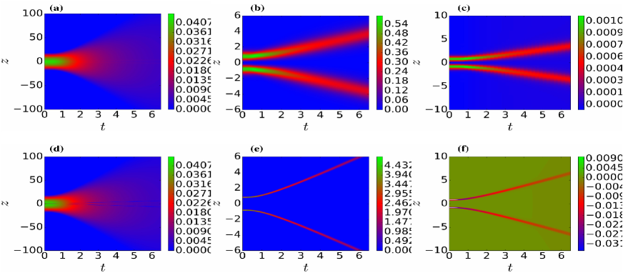
Figure 2: Time-of-flight evolution of BEC density (a,d), excited-impurity density (b,e) and BEC depleted density $n_{\text{B}}\left(z,t\right){}_{\text{DD}}=n_{\text{B}}\left(z,t\right){}_{g_{\text{IB}}}-n_{\text{B}}\left(z,t\right){}_{g_{\text{IB}}=0}$ (c,f) versus time and position for different values of $g_{\text{IB}}=-40$ (a-c), and $g_{\text{IB}}=80$ (d-f) by using the two coupled dimensionless Eqs. (3) and (4) in dimensionless units.

here, the first equation (3) describes the dynamics of the BEC, and the second equation illustrates the dynamics of the SESI. In the above equations, $\tilde{\alpha}=l_{\text{Iz}}/l_{\text{z}}$ has the value 0.808, here $\tilde{G}_{\text{B}}=2N_{\text{B}}\omega_{\text{r}}a_{\text{B}}/\omega_{\text{z}}l_{\text{z}}$, and $\tilde{g}_{\text{IB}}=2a_{\text{IB}}\omega_{\text{r}}f\left(\omega_{\text{Ir}}/\omega_{\text{r}}\right)/\omega_{\text{z}}l_{\text{z}}$ are the dimensionless Rb-Rb and Rb-Cs coupling strengths, respectively. By using above mentioned experimental values, we obtained the dimensionless Rb-Rb and Rb-Cs coupling strengths as $\tilde{G}_{\text{B}}=4.71$ and $\tilde{g}_{\text{IB}}=0.16$, respectively. From here on, we will drop all the tildes for simplicity. To find the numerical excited state of a Cs impurity, we start with a trial excited state wave function for the impurity as summarized in appendix  A, here the impurity dimensionless energy $E_{\text{I}}$ depends upon the dimensionless imaginary time.

In order to determine the equilibrium excited-impurity imprint on the condensate wave function, we solve numerically the two coupled dimensionless quasi 1DGPE (3) for the BEC and the differential equation (4) for the excited-impurity by using the split-operator method Vudragović et al. (2012); Kumar et al. (2015); Lončar et al. (2016); Satarić et al. (2016). In this way, we demonstrate that the ${}^{133}\text{Cs}$ excited-impurity leads to two bumps or two holes at the center of the ${}^{87}\text{Rb}$ BEC density for attractive or repulsive interspecies coupling strength $g_{\text{IB}}$ as displayed in Fig. 1(a) and Fig. 1(b), respectively. For stronger attractive $g_{\text{IB}}$ values two bumps can increase further as depicted in Fig. 1(a), but for strong repulsive $g_{\text{IB}}$ values two dips in the BEC density gets deeper and deeper until BEC fragmented into three parts as illustrated in Fig. 1(b). Additionally, the SESI effective mass increases quadratically for interspecies coupling strength $g_{\text{IB}}$ as presented in appendix  B. In this manuscript, we have utilized the zero-temperature GP mean-field theory, however, as a matter-of-fact, elementary excitations can arise from the thermal and/or quantum fluctuations Griffin (1996), and the BEC dynamics may be considerably affected by the motion of the excited atoms around it (thermal cloud), and by the dynamical BEC depletion Castin and Dum (1997). To give a rough estimate to our reader, first of all, we let that the excited-impurity in our proposed model does not affect the mean-field description of our system. The mean-field approximations hold so long as the impurity-BEC interaction does not significantly deplete the condensate, leading to the condition Astrakharchik and Pitaevskii (2004); Bruderer et al. (2008); Shashi et al. (2014)

$$|a_{\text{IB}}|\xi^{-1}\ll 1.$$ (5)

Here, $\xi^{-1}=l_{\text{r}}/\sqrt{2n_{\text{1D}}a_{\text{B}}}$ is the 1D healing length. The dimensionless peak density of the BEC at the center of the condensate is $\tilde{n}_{\text{1D}}=0.355(0.164)$ for the dimensionless Rb-Rb coupling strength $\tilde{G}_{\text{B}}=10(100)$ and the corresponding value $|a_{\text{IB}}|\xi^{-1}=0.0020(0.0014)$, respectively. Which shows that our treatment of the single excited-impurity in a BEC system neglects the phenomenology of strong-coupling physics, e.g., near a Feshbach resonance Rath and Schmidt (2013), which lies beyond the parameter range of Eq. (5). Therefore, we restrict the following calculation of the validity range of the mean-field analysis to a BEC without any excited-impurity. Additionally, in appendix  C, we regulate how quantum and thermal fluctuations within the Bogoliubov theory restrict the validity range of our mean-field description.

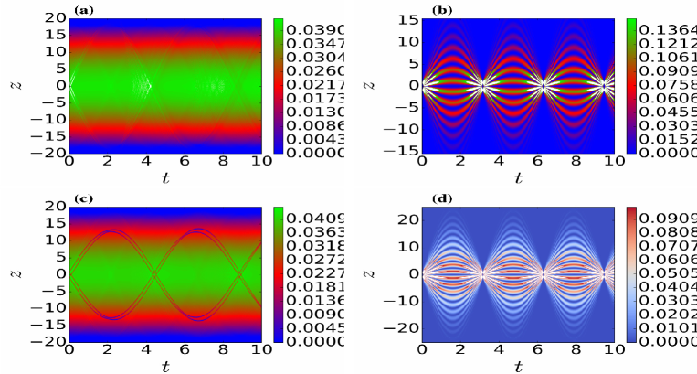
Figure 3: Evolution of the BEC density (a,c) and the excited-impurity density (b,d) in a harmonic trap, when the interspecies interaction strength is switched off, versus time and position for different values of $g_{\text{IB}}=-40$ (a-b) and $g_{\text{IB}}=80$ (c-d) in dimensionless units.

III Dynamics of the BEC and the excited-impurity

To investigate the dynamical evolution of the condensate wave function and the excited-impurity, we investigate numerically two quench scenarios. In the first scenario, we investigate the standard time-of-flight (TOF) expansion after having switched off the external harmonic trap when the excited-impurity and BEC interspecies interaction strength is still present. In the second case, we consider an inverted situation where the excited-impurity and the BEC interspecies interaction strength is turned off by letting the harmonic confinement switched on. This represents an interesting scheme to generate matter waves like shock-waves or solitons depending on either the initial excited-impurity and BEC interaction strength is attractive or repulsive.

In the first scheme, we turn off the magnetic trap at time $t=0$, the BEC and the SESI is allowed to expand in all directions. At $t=0$, the confining potential vanishes, and further acceleration results from inter- and intra-species interactions strength. For the attractive or repulsive interspecies coupling strength, two bumps or dips decay slowly during the temporal evolution as shown in Figs. 2(a) and 2(d). The relative speed of decaying of these bumps or dips from each other is zero. The SESI imprint bumps or dips are not only decaying but also moving away from their stationary positions as demonstrated in Figs. 2(c) and 2(f).

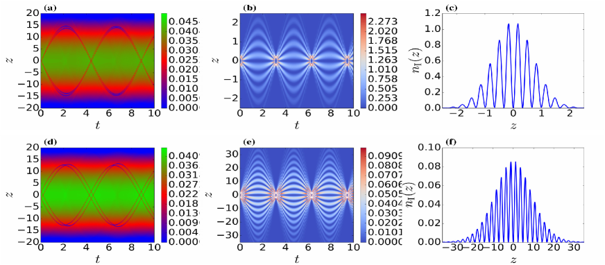
Figure 4: Dynamical evolution of the BEC density (a,d) and the excited-impurity density (b,e), when interspecies interaction strength is switched off, versus time and position for values of $\alpha=0.2$ (a-c) and $\alpha=1.5$(d-f) in dimensionless units. In figure (c) and (f) we plot the excited-impurity density at dimensionless time $t=10$.

In the second scenario, we introduce a numerical model of matter-wave self-interference resulting from the attractive and repulsive interspecies strength is switched off and within a remaining harmonic confinement, which leads to the shock waves and gray quad-solitons, respectively, as predicted in Figs. 3(a) and 3(c). We observed that in every scenario, approximately $t<0.045$ dimensionless time is required to generate shock-waves or quad-solitons as shown in Figs. 3(a) and 3(c), respectively. For an initial attractive interspecies coupling strength $g_{\text{IB}}=-40$, we examine that two excitations of the condensate are generated at the SESI position, which travel in different direction with identical center-of-mass speed, are reflected at the harmonic confinement boundaries and then collide at the SESI position as depicted in Fig. 3(a). We have done different calculations, by changing the value of $g_{\text{IB}}<0$, in all cases, we observed that the appearance of shock wave structures as shown in Fig. 3(a). The density of depleted atoms around shocks becomes, at most, larger than depletion density far away from perturbations. The corresponding excited-impurity self-interference pattern starts breathing with dimensionless frequency $\omega_{I}/\omega_{{\rm z}}=2$ at the center of the harmonic trap as shown in Fig. 3(b). For small attractive/repulsive interspecies scattering strength the excited-impurity self-interference fringes show smaller strength as discussed in appendix  D. We can determine the breathing frequency of the SESI in a harmonic trap by defining the single excited-impurity wave function $\psi_{\text{I}}\left(z,t\right)=\sqrt{2/\left[\sqrt{\pi}A(t)^{3}\right]}\,ze^{-\frac{z^{2}}{2A(t)^{2}}-iz^{2}R(t)},$ here $A(t)$ defines the dimensionless width of the SESI and $R(t)=-A^{\prime}(t)/2\alpha^{2}A(t)$ describes the variational parameter which defines the momentum of the SESI. We write the equation of motion for the width of the excited-impurity by determining the Euler-Lagrangian equation of the system in

$$A^{\prime\prime}(t)-\frac{\alpha^{4}}{A(t)^{3}}+A(t)=0\,.$$ (6)

where the equilibrium state is $A\left(t=0\right)=A_{0}=\alpha$ and $\alpha=l_{\text{Iz}}/l_{\text{z}}$ has the equilibrium value 0.808. We solve Eq. (6) and get the time dependent width of the excited-impurity $A(t)=\sqrt{\left[\alpha^{4}+\left(A_{0}^{4}-\alpha^{4}\right)\cos(2t)+A_{0}^{4}\right]/2A_{0}^{2}}$. Thus, in order to get the excited-impurity out of equilibrium we can let $A_{0}=\alpha\pm\delta$, where $\delta$ is a small quantity. From the time dependent width of the excited-impurity, we identify the dimensionless breathing oscillation frequency to be $\omega_{I}/\omega_{{\rm z}}=2$.

And for the repulsive interspecies coupling strength $g_{\text{IB}}=80$, we inspect gray quad-solitons, traveling with the same speed as shown in Fig. 3(c). In the case of harmonic confinement with a dimensionless potential $V_{\textrm{ext}}=z^{2}/2$, the frequency of the oscillating soliton differs from the trap frequency by a factor $\omega_{s}/\omega_{{\rm z}}=1/\sqrt{2}$ as exhibited in Fig. 3(c), which was predicted in Reinhardt and Clark (1997); Busch and Anglin (2000); Akram and Pelster (2016b, c) and experimentally observed in K.E. Strecker et al. (2002); Al Khawaja et al. (2002). At the maxima of excited-impurity wave function two gray-solitons are generated which have zero relative phase, and they travel in opposite directions as displayed in Fig. 3(c). On the other hand two gray-solitons are generated at the minima of the excited-impurity wave function, they also have zero relative phase from each other and zero phase difference as compared to the two gray-solitons which were created at the maxima of excited-impurity wave function. If two gray-solitons have a relative phase difference of zero, they attract to each other when they come near to each other Aitchison et al. (1991), as demonstrate in Fig. 3(c) near to dimensionless time $t\approx 2.2$. This phenomena happens when two solitons reaches at the trap boundary approximately at the same time $t\approx 2.2$, the latter one tries to cross the first one, therefore they collide with one another and then reflected, and surprisingly this attractive phenomena does not affect the oscillation frequency of the solitons in a harmonic trap as depicted in Fig. 3(c). Furthermore, quad-solitons collide at their originated position and go through each other without any disturbance as exhibited in Fig. 3(c) near to dimensionless time $t\approx 4.2$. On the contrary, the single excited-impurity exhibit self-interference fringes as demonstrated in Fig. 3(d). As excited-impurity wave function has one maxima and one minima, therefore when the repulsive interspecies coupling strength is switched off, then the single excited state impurity self-interference patterns are generated as demonstrated in Fig. 3(d). These self-interference patterns represent a clear evidence for the spatial coherence of excited-impurity, while the special patterns repeat themselves with a unique frequency $\omega_{I}/\omega_{{\rm z}}=2$ as shown in Fig. 3(d), which we calculated by solving Eq. (6). We also find out that the excited-impurity density self interference patterns does not pass through each other at $z=0$, which is quite clear as they do not exhibit solitonic behavior as demonstrated in Figs. 3(b) and 3(d).

To illustrate a more general case for the generation of the solitons by pinning the excited-impurity in the center of the BEC, we investigate different masses impurities, which basically change nothing in our proposed model but the value of parameter $\alpha=\sqrt{m_{\text{I}}/m_{\text{B}}}$. For the value of $\alpha=0.2$, we witness a new kind of phenomena where only two gray-solitons are generated as the distance between the maxima and the minima of the excited-impurity wave function is quite small therefore solitons get the overall shape of the sculpted BEC as depicted in Fig. 4(a). The shape of these gray bi-solitons is totally different than the shape of the solitons for parameter $\alpha=0.808$ as demonstrated in Fig. 3(c). For the case $\alpha=0.2$, near to the trap boundary, soliton does not attract each other, as they express unite identity, as demonstrated in Fig. 4(a). Additionally, these bi-solitons oscillate in a harmonic trap with the same dimensionless frequency $\omega_{s}/\omega_{{\rm z}}=1/\sqrt{2}$ as predicted in the previous case. In Fig. 4(d), we use $\alpha=1.5$, in this scenario, again quad gray-solitons are generated, which reveal similar properties as discussed for the case of $\alpha=0.808$. Furthermore, the SESI interference fringes height decreases with increasing bare mass of the excited-impurity and vise versa as demonstrated in Fig. 4(c) and Fig. 4(f). On the other hand, we observe that the number of interference fringes increases with increasing the bare mass of the excited-impurity as illustrated Fig. 4(c) and Fig. 4(f). Additionally, as the bare mass of the SESI increases, the width of center-of-mass of the solitons decreases as shown in Fig. 4(a) and Fig. 4(d), the reason for this is quite simple and clear as solitons depth increases with increasing mass, therefore, they can not move away from their central position.

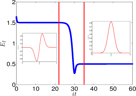
Figure 5: Dimensionless energy decay in dimensionless imaginary time. Here a rectangular widow is separating the transition region from excited to ground state from left to right, respectively. In inlet we plot the excited-impurity and the ground-state wave functions.

IV Discussion

Our studies elucidate the role of single excited state impurity pinned in a ${}^{87}\text{Rb}$ BEC. We model our system in the mean-field regime by writing the one-dimensional two coupled differential equations, this approximation is valid for relatively weak interspecies interaction and for single excited-impurity. We pinned the excited-impurity in the condensate center and diminished its decay by using the quantum zeno effect. We found out that the BEC depletion induced by the single excited state impurity, cause the BEC density to split into three parts. During our calculation, we have found out that the excited-impurity imprint decays marginally for the attractive interspecies coupling strength, and in repulsive interspecies coupling strength, it starts decay significantly as compared to the small value of the interspecies interaction strength. We have used the numerical simulation to analyze generation and the dynamics of gray quad-solitons or bi-solitons in the Bose-Einstein condensate. We disclose that the shape of newly generated solitons depends on the bare mass of the excited state impurity. We would like to remark that even though in our analysis we use an idealized potential for the excited-impurity, but such an approximation is known to, not only, encapsulate the basic physics, but can also be a good approximation to experimental setups.

Appendix A Impurity energy

With $\psi_{\text{I}}\left(z,t\right)=\psi_{\text{I}}\left(z\right)e^{-iE_{\text{I}}t}$, where $E_{\text{I}}$ is the impurity dimensionless energy, we plotted in Fig. 5, the impurity dimensionless energy vs the dimensionless imaginary time when there is no condensate present at the background of the impurity. To find the numerical excited state of a Cs impurity, we start with a trial excited state wave function for the impurity

$$\psi_{\text{I}}\left(z\right)=\sqrt{\frac{2}{\sqrt{\pi}A^{3}}}ze^{-\frac{z^{2}}{2A^{2}}}\,,$$ (7)

here $A$ is the dimensionless width of the first excited state of the wave-packet, for the excited state $A=\alpha$ where $\alpha=l_{\text{Iz}}/l_{\text{z}}$ has the value 0.808. For the single excited state, the excited-impurity state is durable for $it\simeq 70$. It means that in our numerical simulation the excited-impurity can be seen for a specific dimensionless imaginary time interval which later decays to its ground state as shown in Fig. 5.

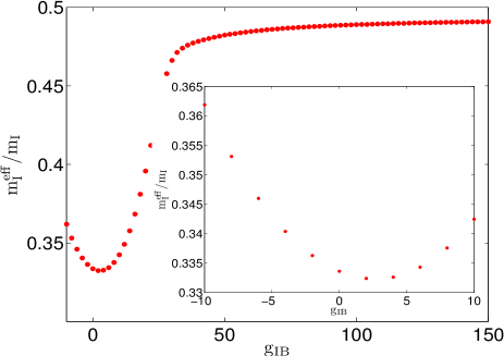
Figure 6: (Color online) Effective mass of ${}^{133}\text{Cs}$ impurity versus the impurity-BEC coupling strength $g_{\text{IB}}$. Inlet shows that effective mass increases quadratically for small impurity-BEC coupling strength $g_{\text{IB}}$ in dimensionless units.

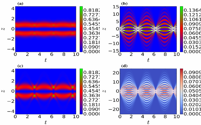
Figure 7: Evolution of the excited-impurity density in a harmonic trap, when the interspecies interaction strength is switched off, versus time and position for different values of interspecies interaction strength (a) $g_{\text{IB}}=-10$, (b) $g_{\text{IB}}=-40$, (c) $g_{\text{IB}}=20$ and (d) $g_{\text{IB}}=80$ in dimensionless units.

Appendix B Effective mass

The effective mass of the excited-impurity is denoted as $m_{\text{I}}^{\text{eff}}=\hbar/\left(l_{\text{Iz}}^{2}\omega_{\text{z}}\right)$, where the excited-impurity oscillator length $l_{\text{Iz}}=\sqrt{2}\sigma$ come from the standard deviation $\sigma=\sqrt{<z^{2}>-<z>^{2}}$, with $<\bullet>=\int\bullet\left|\psi_{\text{I}}(z)\right|^{2}dz$ representing the expectation value. Figure 6 shows the ratio of the effective mass of the ${}^{133}\text{Cs}$ impurity with respect to the bare mass $m_{\text{I}}$, which increases quadratically for interspecies coupling strength $-10<g_{\text{IB}}<10$ as shown in the inlet of Fig. 6, and becomes marginally saturated for interspecies coupling strength $g_{\text{IB}}>80$. Here, we utilize the mean-field regime to determine the effective mass of the excited-impurity. Through this connection, one may extend this work to investigate polaron physics, in order to include the impact of quantum and thermal fluctuations Tempere et al. (2009); Casteels et al. (2011); Santamore and Timmermans (2011); Grusdt and Demler (2015).

Appendix C Mean-field analysis

To give a rough estimate to our reader, first of all we let that the excited-impurity in our proposed model does not affect the mean-field description of our system. Therefore, we restrict the following calculation of the validity range of the mean-field analysis to a BEC without any excited-impurity. In the following, we regulate how quantum and thermal fluctuations within the Bogoliubov theory restrict the validity range of our mean-field description.

Quantum depletion

According to the Bogoliubov theory the three-dimensional quantum fluctuation term is defined in Thomas-Fermi approximation:

$$n_{\text{QF}}^{\text{3D}}\left(\mathbf{r}\right)=n_{\text{0B}}^{\text{3D}}\left(\mathbf{r}\right)-n_{\text{B}}^{\text{3D}}\left(\mathbf{r}\right)=\frac{8}{3\sqrt{\pi}}\left[N_{\text{B}}a_{\text{B}}n_{\text{B}}^{\text{3D}}\left(\mathbf{r}\right)\right]^{3/2}.$$ (8)

We assume an effective one-dimensional setting with $\omega_{\text{z}}\ll\omega_{\text{r}}$, so we decompose the BEC wave-function $\psi_{\text{B}}(\mathbf{r},t)=\psi_{\text{B}}(z,t)\phi_{\text{B}}(\textbf{ r}_{\perp},t)$ with $\textbf{ r}_{\perp}=\left(x,\;y\right)$ and

$$\phi_{\text{B}}(\textbf{ r}_{\perp},t)=\frac{e^{-\frac{x^{2}+y^{2}}{2l_{\text{r}}^{2}}}}{\sqrt{\pi}l_{\text{r}}}e^{-i\omega_{\text{r}}t}\,.$$ (9)

We integrate out the transversal degrees of freedom from equation (8) to get an effective one-dimensional setting

$$n_{\text{QF}}^{\text{1D}}\left(z\right)=n_{\text{0B}}^{\text{1D}}\left(z\right)-n_{\text{B}}^{\text{1D}}\left(z\right)=\frac{16}{9\pi l_{\text{r}}}\left[N_{\text{B}}a_{\text{B}}n_{\text{B}}^{\text{1D}}\left(z\right)\right]^{3/2}.$$ (10)

We know that for larger inter-particle interaction strength the BEC density is characterized by the Thomas-Fermi (TF) profile $n_{\text{B}}^{\text{1D}}\left(z\right)=\frac{\mu^{\text{1D}}}{G_{\text{B}}^{\text{1D}}}\left(1-\frac{z^{2}}{R_{\text{z}}^{2}}\right)$ with $R_{\text{z}}^{2}=\frac{2\mu^{\text{1D}}}{m_{\text{B}}\omega_{\textrm{z}}^{2}}$. With this we calculate the one-dimensional quantum fluctuation depleted term with respect to the number of particles $N_{\text{B}}=200$ by using $N_{\text{QF}}^{\text{1D}}=\int n_{\text{QF}}^{\text{1D}}\left(z\right)dz$ and get

$$\frac{N_{\text{QF}}^{\text{1D}}}{N_{\text{B}}}=\frac{3^{1/3}}{4}\left(\frac{a_{\text{B}}^{4}N_{\text{B}}}{l_{\text{r}}^{2}l_{\text{z}}^{2}}\right)^{1/3}.$$ (11)

We evaluate this relative depletion for the system parameters of our study. With this we obtain from (11) $\frac{N_{\text{QF}}^{\text{1D}}}{N_{\text{B}}}=0.0022$, so that the quantum fluctuations are, indeed, negligible.

Thermal depletion

Correspondingly, the one-dimensional thermal depleted term with respect to the number of particles follows from Bogoliubov theory to be

$$\frac{N_{\text{TF}}^{\text{1D}}}{N_{\text{B}}}=\gamma\left(\frac{T}{T_{\textrm{c}}}\right)^{2}$$ (12)

with the dimensionless prefactor

$$\gamma=\frac{5^{2/5}\pi^{2}}{2^{3/2}\times 3^{3/5}}\left\{\frac{N_{\text{B}}^{1/3}}{\xi\left(3\right)^{8/3}}\frac{a_{\text{B}}^{2}}{l_{\text{r}}^{4/3}l_{\text{z}}^{2/3}}\right\}^{1/5}.$$ (13)

For our system parameters we obtain $\gamma=0.046$ and the critical temperature $T_{\textrm{c}}=\frac{\hbar}{k_{\text{B}}}\left(\omega_{r}^{2}\omega_{\textrm{z}}\frac{N_{\text{B}}}{\xi\left(3\right)}\right)^{1/3}=14.7~{}\text{nK}$. Thus, choosing a reasonable ratio of the thermal depleted term $\frac{N_{\text{TF}}^{\text{1D}}}{N_{\text{B}}}=0.001$, we estimate the temperature of the system to be

$$T=T_{\textrm{c}}\sqrt{\frac{1}{\eta}\frac{N_{\text{TF}}^{\text{1D}}}{N_{\text{B}}}}=2.15~{}\text{nK}$$ (14)

With this we conclude that, if the temperature of the system is lower than $T=2.15~{}\text{nK}$, the thermal fluctuations are not affecting the Bose-Einstein condensate.

Appendix D Excited-impurity self-interference patterns

The single excited-impurity wave packet display self-interference patterns as demonstrated in Fig. 7. As excited-impurity wave function has one maxima and one minima, therefore when the attractive/repulsive interspecies coupling strengths are switched off, then the excited-impurity self-interference patterns are generated. We find out that the excited-impurity density self interference patterns does not pass through each other at $z=0$, which is quite clear as they do not exhibit solitonic behavior as demonstrated in Fig. 7. As we can see from the Fig. 7, for small attractive/repulsive interspecies scattering strength the excited-impurity self-interference fringes demonstrate smaller strength and vise versa.

Appendix E Acknowledgment

We gratefully acknowledge support from the German Academic Exchange Service (DAAD). We thank Thomas Busch and Axel Pelster for insightful comments.

References

- Andrews et al. (1997) M. R. Andrews, C. G. Townsend, H.-J. Miesner, D. S. Durfee, D. M. Kurn, and W. Ketterle, Science 275, 637 (1997).
- Myatt et al. (1997) C. J. Myatt, E. A. Burt, R. W. Ghrist, E. A. Cornell, and C. E. Wieman, Phys. Rev. Lett. 78, 586 (1997).
- Hall et al. (1998) D. S. Hall, M. R. Matthews, J. R. Ensher, C. E. Wieman, and E. A. Cornell, Phys. Rev. Lett. 81, 1539 (1998).
- Kohler and Sols (2002) S. Kohler and F. Sols, Phys. Rev. Lett. 89, 060403 (2002).
- Papp et al. (2008) S. B. Papp, J. M. Pino, and C. E. Wieman, Phys. Rev. Lett. 101, 040402 (2008).
- McCarron et al. (2011) D. J. McCarron, H. W. Cho, D. L. Jenkin, M. P. Köppinger, and S. L. Cornish, Phys. Rev. A 84, 011603 (2011).
- Cazalilla et al. (2011) M. A. Cazalilla, R. Citro, T. Giamarchi, E. Orignac, and M. Rigol, Rev. Mod. Phys. 83, 1405 (2011).
- He et al. (2015) L. He, A. Ji, and W. Hofstetter, Phys. Rev. A 92, 023630 (2015).
- Ho and Shenoy (1996) T.-L. Ho and V. B. Shenoy, Phys. Rev. Lett. 77, 3276 (1996).
- Pu and Bigelow (1998) H. Pu and N. P. Bigelow, Phys. Rev. Lett. 80, 1130 (1998).
- W. S. Bakr et al. (2009) W. S. Bakr, J. I. Gillen, A. Peng, S. Folling, and M. Greiner, Nature (London) 462, 74 (2009).
- J. F. Sherson et al. (2010) J. F. Sherson, C. Weitenberg, M. Endres, M. Cheneau, I. Bloch, and S. Kuhr, Nature (London) 467, 68 (2010).
- Serwane et al. (2011) F. Serwane, G. Zürn, T. Lompe, T. B. Ottenstein, A. N. Wenz, and S. Jochim, Science 332, 336 (2011).
- Ratschbacher Lothar et al. (2012) Ratschbacher Lothar, Zipkes Christoph, Sias Carlo, and Köhl Michael, Nature Phys. 8, 649 (2012).
- Schurer et al. (2014) J. M. Schurer, P. Schmelcher, and A. Negretti, Phys. Rev. A 90, 033601 (2014).
- Schurer et al. (2015) J. M. Schurer, A. Negretti, and P. Schmelcher, New J. Phys. 17, 083024 (2015).
- Schirotzek et al. (2009) A. Schirotzek, C.-H. Wu, A. Sommer, and M. W. Zwierlein, Phys. Rev. Lett. 102, 230402 (2009).
- Palzer et al. (2009) S. Palzer, C. Zipkes, C. Sias, and M. Köhl, Phys. Rev. Lett. 103, 150601 (2009).
- C. Zipkes et al. (2010) C. Zipkes, S. Palzer, C. Sias, and M. Köhl, Nature (London) 464, 388 (2010).
- Schmid et al. (2010) S. Schmid, A. Härter, and J. H. Denschlag, Phys. Rev. Lett. 105, 133202 (2010).
- Micheli et al. (2004) A. Micheli, A. J. Daley, D. Jaksch, and P. Zoller, Phys. Rev. Lett. 93, 140408 (2004).
- Klein and Fleischhauer (2005) A. Klein and M. Fleischhauer, Phys. Rev. A 71, 033605 (2005).
- Daley et al. (2004) A. J. Daley, P. O. Fedichev, and P. Zoller, Phys. Rev. A 69, 022306 (2004).
- Griessner et al. (2006) A. Griessner, A. J. Daley, S. R. Clark, D. Jaksch, and P. Zoller, Phys. Rev. Lett. 97, 220403 (2006).
- Klein et al. (2007) A. Klein, M. Bruderer, S. R. Clark, and D. Jaksch, New J. Phys. 9, 411 (2007).
- Casteels et al. (2011) W. Casteels, J. Tempere, and J. T. Devreese, Phys. Rev. A 84, 063612 (2011).
- Santamore and Timmermans (2011) D. H. Santamore and E. Timmermans, New J. Phys. 13, 103029 (2011).
- Hohmann et al. (2015) M. Hohmann, F. Kindermann, B. Gänger, T. Lausch, D. Mayer, F. Schmidt, and A. Widera, EPJ Quant. Technol. 2, 23 (2015).
- Kinoshita et al. (2006) T. Kinoshita, T. Wenger, and D. S. Weiss, Nature (London) 440, 900 (2006).
- Ng and Bose (2008) H. T. Ng and S. Bose, Phys. Rev. A 78, 023610 (2008).
- A. D. Lercher et al. (2011) A. D. Lercher, T. Takekoshi, M. Debatin, B. Schuster, R. Rameshan, F. Ferlaino, R. Grimm, and H.-C. Nägerl, Eur. Phys. J. D 65, 3 (2011).
- Spethmann et al. (2012a) N. Spethmann, F. Kindermann, S. John, C. Weber, D. Meschede, and A. Widera, Appl. Phys. B 106, 513 (2012a).
- Spethmann et al. (2012b) N. Spethmann, F. Kindermann, S. John, C. Weber, D. Meschede, and A. Widera, Phys. Rev. Lett. 109, 235301 (2012b).
- J. B. Balewski et al. (2013) J. B. Balewski, A. T. Krupp, A. Gaj, D. Peter, H. P. Buchler, R. Low, S. Hofferberth, and T. Pfau, Nature (London) 502, 664 (2013).
- Akram and Pelster (2016a) J. Akram and A. Pelster, Phys. Rev. A 93, 033610 (2016a).
- Pilch et al. (2009) K. Pilch, A. D. Lange, A. Prantner, G. Kerner, F. Ferlaino, H.-C. Nägerl, and R. Grimm, Phys. Rev. A 79, 042718 (2009).
- Takekoshi et al. (2012) T. Takekoshi, M. Debatin, R. Rameshan, F. Ferlaino, R. Grimm, H.-C. Nägerl, C. R. Le Sueur, J. M. Hutson, P. S. Julienne, S. Kotochigova, and E. Tiemann, Phys. Rev. A 85, 032506 (2012).
- Vidanović et al. (2011) I. Vidanović, A. Balaž, H. Al-Jibbouri, and A. Pelster, Phys. Rev. A 84, 013618 (2011).
- Wang et al. (2014) T. Wang, X.-F. Zhang, F. E. A. d. Santos, S. Eggert, and A. Pelster, Phys. Rev. A 90, 013633 (2014).
- Itano et al. (1990) W. M. Itano, D. J. Heinzen, J. J. Bollinger, and D. J. Wineland, Phys. Rev. A 41, 2295 (1990).
- Fischer et al. (2001) M. C. Fischer, B. Gutiérrez-Medina, and M. G. Raizen, Phys. Rev. Lett. 87, 040402 (2001).
- Leibfried et al. (2003) D. Leibfried, R. Blatt, C. Monroe, and D. Wineland, Rev. Mod. Phys. 75, 281 (2003).
- Vudragović et al. (2012) D. Vudragović, I. Vidanović, A. Balaž, P. Muruganandam, and S. K. Adhikari, Comp. Phys. Commun. 183, 2021 (2012).
- Kumar et al. (2015) R. K. Kumar, L. E. Young-S., D. Vudragović, A. Balaž, P. Muruganandam, and S. Adhikari, Comput. Phys. Commun. 195, 117 (2015).
- Lončar et al. (2016) V. Lončar, A. Balaž, A. Bogojević, S. Škrbić, P. Muruganandam, and S. K. Adhikari, Comput. Phys. Commun. 200, 406 (2016).
- Satarić et al. (2016) B. Satarić, V. Slavnić, A. Belić, A. Balaž, P. Muruganandam, and S. K. Adhikari, Comput. Phys. Commun. 200, 411 (2016).
- Griffin (1996) A. Griffin, Phys. Rev. B 53, 9341 (1996).
- Castin and Dum (1997) Y. Castin and R. Dum, Phys. Rev. Lett. 79, 3553 (1997).
- Astrakharchik and Pitaevskii (2004) G. E. Astrakharchik and L. P. Pitaevskii, Phys. Rev. A 70, 013608 (2004).
- Bruderer et al. (2008) M. Bruderer, A. Klein, S. R. Clark, and D. Jaksch, New Journal of Physics 10, 033015 (2008).
- Shashi et al. (2014) A. Shashi, F. Grusdt, D. A. Abanin, and E. Demler, Phys. Rev. A 89, 053617 (2014).
- Rath and Schmidt (2013) S. P. Rath and R. Schmidt, Phys. Rev. A 88, 053632 (2013).
- Reinhardt and Clark (1997) W. P. Reinhardt and C. W. Clark, J. Phys. B: At., Mol. Opt. Phys. 30, L785 (1997).
- Busch and Anglin (2000) T. Busch and J. R. Anglin, Phys. Rev. Lett. 84, 2298 (2000).
- Akram and Pelster (2016b) J. Akram and A. Pelster, Las. Phys. 26, 065501 (2016b).
- Akram and Pelster (2016c) J. Akram and A. Pelster, Phys. Rev. A 93, 023606 (2016c).
- K.E. Strecker et al. (2002) K.E. Strecker, G.B. Partridge, A.G. Truscott, and R.G. Hulet, Nature (London) 417, 150 (2002).
- Al Khawaja et al. (2002) U. Al Khawaja, H. T. C. Stoof, R. G. Hulet, K. E. Strecker, and G. B. Partridge, Phys. Rev. Lett. 89, 200404 (2002).
- Aitchison et al. (1991) J. S. Aitchison, A. M. Weiner, Y. Silberberg, D. E. Leaird, M. K. Oliver, J. L. Jackel, and P. W. E. Smith, Opt. Lett. 16, 15 (1991).
- Tempere et al. (2009) J. Tempere, W. Casteels, M. K. Oberthaler, S. Knoop, E. Timmermans, and J. T. Devreese, Phys. Rev. B 80, 184504 (2009).
- Grusdt and Demler (2015) F. Grusdt and E. Demler, ArXiv:1510.04934 (2015).