Nonlinear waves in magnetized quark matter and the reduced Ostrovsky equation

Abstract

We study nonlinear waves in a nonrelativistic ideal and cold quark gluon plasma immersed in a strong uniform magnetic field. In the context of nonrelativistic hydrodynamics with an external magnetic field we derive a nonlinear wave equation for baryon density perturbations, which can be written as a reduced Ostrovsky equation. We find analytical solutions and identify the effects of the magnetic field.

I Introduction

There is a strong evidence that quark gluon plasma (QGP) has been observed in heavy ion collisions at RHIC and at LHC qgp1 ; qgp2 . Deconfined quark matter may also exist in the core of compact stars qgp3 . Waves may be formed in the QGP w1 ; w2 . In heavy ion collisions waves may be produced, for example, by fluctuations in baryon number, energy density or temperature caused by inhomogeneous initial conditions w2 .

In order to study waves, it is very often assumed that they represent small perturbations in a fluid and hence one can linearize the equations of hydrodynamics and find their solutions, which are linear waves. Alternatively, instead of linearization we may use another procedure, called Reductive Perturbation Method (RPM) rpm , which preserves the nonlinearity of the original equations. This leads to nonlinear differential equations, whose solution describe nonlinear waves, such as solitons. In a series of works werev ; weset we studied the existence and properties of nonlinear waves in hadronic matter and in a quark gluon plasma as well.

The existence and effects of a magnetic field in quark stars has been studied since long time ago mag1 and became a hot topic in our days. In a different context, about ten years ago mag2 it was realized that a very strong magnetic field might be produced in relativistic heavy ion collisions and it might have some effect on the quark gluon plasma phase. A natural question is then: what it the effect of the magnetic field on the waves propagating through the QGP ?

In a previous work we17 we studied the conditions for an ideal, cold and magnetized quark gluon plasma (QGP) to support stable and causal perturbations. These perturbations were considered in the linear approach and the QGP was treated with nonrelativistic hydrodynamics. We have derived the dispersion relation for density and velocity perturbations. The magnetic field was included both in the equation of state and in the equations of motion, where the term of the Lorentz force was considered. We have used three equations of state: a generic non-relativistic one, the MIT bag model EOS (for weak and strong magnetic field) and the mQCD EOS. The anisotropy effects caused by the B field were also manifest in the parallel and perpendicular sound speeds. We found that the existence of a strong magnetic field does not lead to instabilities in the velocity and density waves. Moreover, in most of the considered cases the propagation of these waves was found to respect causality. However causality might be violated in the strong field regime. The onset of causality violation might happen at very large densities and/or large values of the wave length (small values of the wavenumber $k$). The magnetic field changes the pressure, the energy density and the speed of sound. It also changes the equations of hydrodynamics. One of the conclusions of Ref. we17 is that the changes in hydrodynamics are by far more important than the changes in the equation of state.

In the present study we extend our previous work to the case of nonlinear waves. We will investigate the effects of a strong and uniform magnetic field on nonlinear baryon density perturbations in an ideal and magnetized quark gluon plasma. We consider the magnetic field in the EOS and also in the Euler equation, which requires special attention in the RPM rpm formalism. Our study could be applied to the deconfined cold quark matter in compact stars and to the cold quark gluon plasma formed in heavy ion collisions at intermediate energies at FAIR fair or NICA nica . We go beyond the linear approach used in we17 and improve the nonlinear treatment used in w2 , now including the strong magnetic field effects.

Some work along this line was already published in azam , where the authors concluded that increasing the magnetic field leads to a reduction in the amplitude of the nonlinear waves. More recently javi17 , perturbations in a cold QGP were studied with nonrelativistic hydrodynamics with magnetic field effects in a nonlinear approach. Solitonic density waves were found as solutions of a modified nonlinear Schrodinger equation. The magnetic field was found to increase the phase speed of the soliton and to reduce its width. We will discuss below the differences between our study and the above mentioned works.

II Nonrelativistic hydrodynamics

We start from the nonrelativistic Euler equation land with an external uniform magnetic field. The same magnetic field affects the thermodynamical quantities appearing in the equation of state, as in we17 . The magnetic field of intensity $B$ is chosen to be in the $z-$direction and hence $\vec{B}=B\hat{z}$ . The three fermions species considered are the quarks: up ($u$), down ($d$) and strange ($s$) with the following respectively charges $Q_{u}=2\,Q_{e}/3$, $Q_{d}=-\,Q_{e}/3$ and $Q_{s}=-\,Q_{e}/3$, where $Q_{e}=0.08542$ is the absolute value of the electron charge in natural units glend . Because of the external magnetic field, particles with different charges may assume different trajectories azam ; multif and this justifies the use of the multi-fluid approach azam ; multif ; we17 . Throughout this work, we employ natural units ($\hbar=c=1$) and the metric used is $g^{\mu\nu}=\textrm{diag}(+,-,-,-)$.

Starting from the hydrodynamics equations discussed in we17 , and The Euler equation for the quark of flavor $f$ (f=u,d,s) reads:

$${\rho_{m\,f}}\Bigg{[}{\frac{\partial\vec{v_{f}}}{\partial t}}+(\vec{v_{f}}\cdot\vec{\nabla})\vec{v_{f}}\Bigg{]}=-\vec{\nabla}p+{\rho_{c\,f}}\Big{(}\vec{v_{f}}\times\vec{B}\Big{)}$$ (1)

where ${\rho_{m\,f}}$ is the quark mass density. The charge density of the quark flavor $f$ is $\rho_{c\,f}$ azam and the masses are: $m_{u}=2.2\,MeV$, $m_{d}=4.7\,MeV$, $m_{s}=96\,MeV$ and $m_{e}=0.5\,MeV$ pdg .

The continuity equation for the mass density $\rho_{m\,f}$ island :

$${\frac{\partial\rho_{m\,f}}{\partial t}}+\vec{\nabla}\cdot(\rho_{m\,f}\,{\vec{v_{f}}})=0$$ (2)

The relationship between the mass density and the baryon density is ${\rho_{m}}_{f}=3m_{f}\,\,{\rho_{B}}_{f}$ we17 . The charge density for each quark is given by ${\rho_{c}}_{u}=2Q_{e}\,{\rho_{B}}_{u}$  ,   ${\rho_{c}}_{d}=-Q_{e}\,{\rho_{B}}_{d}$    and    ${\rho_{c}}_{s}=-Q_{e}\,{\rho_{B}}_{s}$ . In general we write ${\rho_{c}}_{f}=3\,{Q_{f}}\,{\rho_{B}}_{f}$ for each quark $f$.

III Equation of state

In general, the equation of state (EOS) of the quark gluon plasma can be written as a relation between pressure $p$ and energy density $\epsilon$: $p={c_{s}}^{2}\epsilon$, where $c_{s}$ is the speed of sound. As previously studied in we17 ; we16 ; soundes , when the fluid is immersed in an external uniform magnetic field, the pressure splits into a parallel (with respect to the direction of the external field), $p_{\parallel}$, and a perpendicular component, $p_{\perp}$. We have thus a parallel (${c_{s}}_{\parallel}$) and a perpendicular (${c_{s}}_{\perp}$) speed of sound, given by we17 ; we16 ; soundes :

$${({c_{s}}_{\parallel})}^{2}={\frac{\partial p_{\parallel}}{\partial\varepsilon}}\hskip 28.45274pt\textrm{and}\hskip 28.45274pt{({c_{s}}_{\perp})}^{2}={\frac{\partial p_{\perp}}{\partial\varepsilon}}$$ (3)

and hence $p_{\parallel}\approx{({c_{s}}_{\parallel})}^{2}\,\varepsilon$   and   $p_{\perp}\approx{({c_{s}}_{\perp})}^{2}\,\varepsilon$  . The pressure gradient can then be written as:

$$\vec{\nabla}{p}=\Bigg{(}{\frac{\partial{p}_{\perp}}{\partial x}}\,,\,{\frac{\partial{p}_{\perp}}{\partial y}}\,,\,{\frac{\partial{p}_{\parallel}}{\partial z}}\Bigg{)}$$ (4)

III.1 The nonrelativistic equation of state

As in we17 , we take here the limit w2 : $\varepsilon\cong{\rho_{m}}$. Since ${\rho_{m}}=3m_{f}\,{\rho_{B}}_{f}$ and remembering that the pressure is anisotropic, the pressure gradient (4) for the quark of flavor f is given by we17 :

$$\vec{\nabla}p=3m_{f}\Bigg{(}{({c_{s}}_{\perp})}^{2}\,{\frac{\partial{{\rho_{B}}_{f}}}{\partial x}}\,,\,{({c_{s}}_{\perp})}^{2}\,{\frac{\partial{{\rho_{B}}_{f}}}{\partial y}}\,,\,{({c_{s}}_{\parallel})}^{2}\,{\frac{\partial{{\rho_{B}}_{f}}}{\partial z}}\Bigg{)}$$ (5)

III.2 The improved MIT equation of state

The EOS which we call mQCD was derived in we11 and used in we16 and also in we17 . The energy density ($\varepsilon$), the parallel pressure ($p_{f\,\parallel}$) and the perpendicular pressure ($p_{f\,\perp}$), are given respectively by we16 ; we17 :

$$\varepsilon={\frac{27{g_{h}}^{2}}{16{m_{G}}^{2}}}\,({{\rho_{B}}})^{2}+{\mathcal{B}}_{QCD}+{\frac{B^{2}}{8\pi}}+\sum_{f=u}^{d,s}{\frac{|Q_{f}|B}{2\pi^{2}}}\sum_{n=0}^{n^{f}_{max}}3(2-\delta_{n0})\int_{0}^{k^{f}_{z,F}}dk_{z}\sqrt{m_{f}^{2}+k_{z}^{2}+2n|Q_{f}|B}\,,$$ (6)

$$p_{\parallel}={\frac{27{g_{h}}^{2}}{16{m_{G}}^{2}}}\,({{\rho_{B}}})^{2}-{\mathcal{B}}_{QCD}-{\frac{B^{2}}{8\pi}}+\sum_{f=u}^{d,s}{\frac{|Q_{f}|B}{2\pi^{2}}}\sum_{n=0}^{n^{f}_{max}}3(2-\delta_{n0})\int_{0}^{k^{f}_{z,F}}dk_{z}\,{\frac{{k_{z}}^{2}}{\sqrt{m_{f}^{2}+k_{z}^{2}+2n|Q_{f}|B}}}$$ (7)

and

$$p_{\perp}={\frac{27{g_{h}}^{2}}{16{m_{G}}^{2}}}\,({{\rho_{B}}})^{2}-{\mathcal{B}}_{QCD}+{\frac{B^{2}}{8\pi}}+\sum_{f=u}^{d,s}{\frac{|Q_{f}|^{2}B^{2}}{2\pi^{2}}}\sum_{n=0}^{n^{f}_{max}}3(2-\delta_{n0})n\int_{0}^{k^{f}_{z,F}}{\frac{dk_{z}}{\sqrt{m_{f}^{2}+k_{z}^{2}+2n|Q_{f}|B}}}$$ (8)

The baryon density ($\rho_{B}$) is given by we16 ; we17 :

$$\rho_{B}=\sum_{f=u}^{d,s}\,{\frac{|Q_{f}|B}{2\pi^{2}}}\,\sum_{n=0}^{n^{f}_{max}}(2-\delta_{n0})\,\sqrt{{\nu_{f}}^{2}-m_{f}^{2}-2n|Q_{f}|B}\hskip 19.91684pt\textrm{with}\hskip 14.22636ptn\leq n^{f}_{max}=int\Bigg{[}{\frac{{\nu_{f}}^{2}-m_{f}^{2}}{2|Q_{f}|B}}\Bigg{]}$$ (9)

where ${\it{int}}[a]$ denotes the integer part of $a$ and ${\nu_{f}}$ is the chemical potential for the quark $f$. As in we16 we define $\xi\equiv g_{h}/m_{G}$. Choosing $\xi=0$ we recover the MIT EOS. For a given magnetic field intensity, we choose the values for the chemical potentials ${\nu_{f}}$ which determine the density $\rho_{B}$. We also choose the other parameters: $\xi$ and ${\mathcal{B}}_{QCD}$. In this case the pressure gradient (4) becomes

$$\vec{\nabla}p=\Bigg{(}{\frac{27{g_{h}}^{2}}{8{m_{G}}^{2}}}\Bigg{)}\Bigg{(}{\rho_{B}}_{f}\,{\frac{\partial{{\rho_{B}}_{f}}}{\partial x}}\,,\,{\rho_{B}}_{f}\,{\frac{\partial{{\rho_{B}}_{f}}}{\partial y}}\,,\,{\rho_{B}}_{f}\,{\frac{\partial{{\rho_{B}}_{f}}}{\partial z}}\Bigg{)}$$ (10)

IV Nonlinear waves

Now we apply the Reductive Perturbation Method (RPM) rpm ; w2 ; weset ; javi17 ; azam to the basic equations of hydrodynamics (1) and (2) to obtain the nonlinear wave equations that govern the baryon density perturbations. The RPM technique goes beyond the linearization approach and preserves nonlinear terms in the wave equations. The background density, upon which small perturbations occur, is defined by $\rho_{0}$, and it is usually given in terms of the ordinary nuclear matter density $\rho_{N}=0.17\,fm^{-3}$.

According to the RPM technique we rewrite the equations (1) changing variables and going from the $(x,y,z,t)$ space to the $(X,Y,Z,T)$ space using the “stretched coordinates” defined by w2 ; weset : $X=\sigma^{1/2}(x-{c_{s\,\perp}}\,t)\hskip 2.84544pt,\hskip 5.69046ptY=\sigma\,y\hskip 2.84544pt,\hskip 5.69046ptZ=\sigma\,z\hskip 14.22636pt\textrm{and}\hskip 14.22636ptT=\sigma^{3/2}\,t$. In our approach, following the RPM algebraic procedure rpm ; weset we apply the following transformation to the magnetic field: $B=\sigma\,\tilde{B}$. In this way, we obtain the equations (1) and (2) in the $(X,Y,Z,T)$ space containing the (small) parameter $\sigma$, which is the expansion parameter of the dimensionless density and dimensionless velocities:

$$\hat{\rho}_{B\,f}(x,y,z,t)={\frac{\rho_{B\,f}(x,y,z,t)}{\rho_{0}}}=1+\sigma{\rho_{f}}_{1}(x,y,z,t)+\sigma^{2}{\rho_{f}}_{2}(x,y,z,t)+\sigma^{3}{\rho_{f}}_{3}(x,y,z,t)+\dots\,,$$ (11)

$${\hat{v}_{f\,x}}(x,y,z,t)={\frac{{v}_{f\,x}(x,y,z,t)}{{c_{s\,\perp}}}}=\sigma{{v_{{f}\,x}}_{1}}(x,y,z,t)+\sigma^{2}{{v_{{f}\,x}}_{2}}(x,y,z,t)+\sigma^{3}{{v_{{f}\,x}}_{3}}(x,y,z,t)+\dots\,,$$ (12)

$${\hat{v}_{f\,y}}(x,y,z,t)={\frac{{v}_{f\,y}(x,y,z,t)}{{c_{s\,\perp}}}}=\sigma^{3/2}{{v_{{f}\,y}}_{1}}(x,y,z,t)+\sigma^{2}{{v_{{f}\,y}}_{2}}(x,y,z,t)+\sigma^{5/2}{{v_{{f}\,y}}_{3}}(x,y,z,t)+\dots$$ (13)

and

$${\hat{v}_{f\,z}}(x,y,z,t)={\frac{{v}_{f\,z}(x,y,z,t)}{{c_{s\,\parallel}}}}=\sigma^{3/2}{{v_{{f}\,z}}_{1}}(x,y,z,t)+\sigma^{2}{{v_{{f}\,z}}_{2}}(x,y,z,t)+\sigma^{5/2}{{v_{{f}\,z}}_{3}}(x,y,z,t)+\dots$$ (14)

Next we use (11) to (14) to rewrite (1) and (2). We then neglect terms proportional to $\sigma^{n}$ for $n>2$ and collect the remaining terms in a power series of $\sigma$, $\sigma^{3/2}$ and $\sigma^{2}$, solving them in order to obtain an equation in the $(X,Y,Z,T)$ space. This equation is finally written back in the usual $(x,y,z,t)$ space, yielding the nonlinear wave equation for the baryon density perturbation.

The continuity equation (2) in the RPM gives:

$$\sigma\Bigg{\{}-{\frac{\partial{{\rho_{f}}_{1}}}{\partial X}}+{\frac{\partial{{v_{f\,x}}_{1}}}{\partial X}}\Bigg{\}}+\sigma^{2}\Bigg{\{}-{\frac{\partial{{\rho_{f}}_{2}}}{\partial X}}+{\frac{\partial{{v_{f\,x}}_{2}}}{\partial X}}+{\frac{1}{({c_{s\,\perp}})}}{\frac{\partial{{\rho_{f}}_{1}}}{\partial T}}+{\rho_{f}}_{1}{\frac{\partial{{v_{f\,x}}_{1}}}{\partial X}}+{v_{f\,x}}_{1}{\frac{\partial{{\rho_{f}}_{1}}}{\partial X}}$$

$$+{\frac{\partial{{v_{f\,y}}_{1}}}{\partial Y}}+\Bigg{(}{\frac{{c_{s\,\parallel}}}{{c_{s\,\perp}}}}\Bigg{)}{\frac{\partial{{v_{f\,z}}_{1}}}{\partial Z}}\Bigg{\}}=0$$ (15)

and the Euler equation (1) will be studied in following subsections.

IV.1 Nonrelativistic EOS

Applying the RPM procedure to Eq. (1) and using (5), we obtain the following set of equations in powers of the $\sigma$ parameter:

$$\sigma\Bigg{\{}-{\frac{\partial{{v_{f\,x}}_{1}}}{\partial X}}+{\frac{\partial{{\rho_{f}}_{1}}}{\partial X}}\Bigg{\}}$$

$$+\sigma^{2}\Bigg{\{}-{\frac{\partial{{v_{{f}\,x}}_{2}}}{\partial X}}+{\frac{1}{({c_{s\,\perp}})}}{\frac{\partial{{v_{f\,x}}_{1}}}{\partial T}}+\,{v_{f\,x}}_{1}\,{\frac{\partial{{v_{f\,x}}_{1}}}{\partial X}}-{\rho_{{f}}}_{1}\,{\frac{\partial{{v_{f\,x}}_{1}}}{\partial X}}+{\frac{\partial{{\rho_{f}}_{2}}}{\partial X}}-{\frac{Q_{f}\,\tilde{B}}{m_{f}\,({c_{s\,\perp}})}}{v_{f\,y}}_{1}\Bigg{\}}=0\,,$$ (16)

$$\sigma^{3/2}\Bigg{\{}-{\frac{\partial{{v_{f\,y}}_{1}}}{\partial X}}+{\frac{\partial{{\rho_{f}}_{1}}}{\partial Y}}+{\frac{Q_{f}\,\tilde{B}}{m_{f}\,({c_{s\,\perp}})}}{v_{f\,x}}_{1}\Bigg{\}}+\sigma^{2}\Bigg{\{}-{\frac{\partial{{v_{f\,y}}_{2}}}{\partial X}}\Bigg{\}}=0$$ (17)

and

$$\sigma^{3/2}\Bigg{\{}-{\frac{\partial{{v_{f\,z}}_{1}}}{\partial X}}+\Bigg{(}{\frac{{c_{s\,\parallel}}}{{c_{s\,\perp}}}}\Bigg{)}{\frac{\partial{{\rho_{f}}_{1}}}{\partial Z}}\Bigg{\}}+\sigma^{2}\Bigg{\{}-{\frac{\partial{{v_{f\,z}}_{2}}}{\partial X}}\Bigg{\}}=0$$ (18)

Solving the equations (15) to (18) we arrive at:

$${\frac{\partial}{\partial X}}\Bigg{[}{\frac{\partial{{\rho_{f}}_{1}}}{\partial T}}+({c_{s\,\perp}})\,{\rho_{f}}_{1}{\frac{\partial{{\rho_{f}}_{1}}}{\partial X}}\Bigg{]}+{\frac{({c_{s\,\perp}})}{2}}\Bigg{[}{\frac{\partial^{2}{{\rho_{f}}_{1}}}{\partial Y^{2}}}+\Bigg{(}{\frac{{c_{s\,\parallel}}}{{c_{s\,\perp}}}}\Bigg{)}^{2}{\frac{\partial^{2}{{\rho_{f}}_{1}}}{\partial Z^{2}}}\Bigg{]}={\frac{(Q_{f}\,\tilde{B})^{2}}{2{m_{f}}^{2}\,({c_{s\,\perp}})}}{\rho_{f}}_{1}$$ (19)

Writing (19) back in the cartesian space we obtain the following wave equation:

$${\frac{\partial}{\partial x}}\Bigg{[}{\frac{\partial}{\partial t}}{\delta\rho_{B}}_{f}+({c_{s\,\perp}}){\frac{\partial}{\partial x}}{\delta\rho_{B}}_{f}+({c_{s\,\perp}}){\delta\rho_{B}}_{f}{\frac{\partial}{\partial x}}{\delta\rho_{B}}_{f}\Bigg{]}$$

$$+{\frac{({c_{s\,\perp}})}{2}}\Bigg{[}{\frac{\partial^{2}}{\partial y^{2}}}{\delta\rho_{B}}_{f}+\Bigg{(}{\frac{{c_{s\,\parallel}}}{{c_{s\,\perp}}}}\Bigg{)}^{2}{\frac{\partial^{2}}{\partial z^{2}}}{\delta\rho_{B}}_{f}\Bigg{]}={\frac{(Q_{f}\,B)^{2}}{2{m_{f}}^{2}\,({c_{s\,\perp}})}}{\delta\rho_{B}}_{f}$$ (20)

where ${\delta\rho_{B}}_{f}\equiv\sigma{\rho_{f}}_{1}$ is the baryon density perturbation on the background $\rho_{0}$, as can be seen in (11).

Introducing the variable weset :

$$\xi=x+y+z$$ (21)

the equation (20) becomes:

$${\frac{\partial}{\partial\xi}}\Bigg{\{}{\frac{\partial}{\partial t}}{\delta\rho_{B}}_{f}+\Bigg{[}{\frac{3}{2}}({c_{s\,\perp}})+{\frac{({c_{s\,\parallel}})^{2}}{2({c_{s\,\perp}})}}\Bigg{]}{\frac{\partial}{\partial\xi}}{\delta\rho_{B}}_{f}+({c_{s\,\perp}}){\delta\rho_{B}}_{f}{\frac{\partial}{\partial\xi}}{\delta\rho_{B}}_{f}\Bigg{\}}={\frac{(Q_{f}\,B)^{2}}{2{m_{f}}^{2}\,({c_{s\,\perp}})}}{\delta\rho_{B}}_{f}$$ (22)

IV.2 mQCD

Repeating the steps described in the last subsection and using (10), we obtain:

$$\sigma\Bigg{\{}-{\frac{\partial{{v_{f\,x}}_{1}}}{\partial X}}+\Bigg{(}{\frac{9\,{g_{h}}^{2}\,{\rho_{0}}}{8\,m_{f}\,{m_{G}}^{2}\,({c_{s\,\perp}})^{2}}}\Bigg{)}{\frac{\partial{{\rho_{f}}_{1}}}{\partial X}}\Bigg{\}}+\sigma^{2}\Bigg{\{}-{\frac{\partial{{v_{{f}\,x}}_{2}}}{\partial X}}+{\frac{1}{({c_{s\,\perp}})}}{\frac{\partial{{v_{f\,x}}_{1}}}{\partial T}}+{v_{f\,x}}_{1}\,{\frac{\partial{{v_{f\,x}}_{1}}}{\partial X}}$$

$$-{\rho_{{f}}}_{1}\,{\frac{\partial{{v_{f\,x}}_{1}}}{\partial X}}+{\rho_{{f}}}_{1}\,{\frac{\partial{{\rho_{f}}_{1}}}{\partial X}}+\Bigg{(}{\frac{9\,{g_{h}}^{2}\,{\rho_{0}}}{8\,m_{f}\,{m_{G}}^{2}\,({c_{s\,\perp}})^{2}}}\Bigg{)}{\frac{\partial{{\rho_{f}}_{2}}}{\partial X}}-{\frac{Q_{f}\,\tilde{B}}{m_{f}\,({c_{s\,\perp}})}}{v_{f\,y}}_{1}\Bigg{\}}=0\,,$$ (23)

$$\sigma^{3/2}\Bigg{\{}-{\frac{\partial{{v_{f\,y}}_{1}}}{\partial X}}+\Bigg{(}{\frac{9\,{g_{h}}^{2}\,{\rho_{0}}}{8\,m_{f}\,{m_{G}}^{2}\,({c_{s\,\perp}})^{2}}}\Bigg{)}{\frac{\partial{{\rho_{f}}_{1}}}{\partial Y}}+{\frac{Q_{f}\,\tilde{B}}{m_{f}\,({c_{s\,\perp}})}}{v_{f\,x}}_{1}\Bigg{\}}+\sigma^{2}\Bigg{\{}-{\frac{\partial{{v_{f\,y}}_{2}}}{\partial X}}\Bigg{\}}=0$$ (24)

and

$$\sigma^{3/2}\Bigg{\{}-\Bigg{(}{\frac{{c_{s\,\parallel}}}{{c_{s\,\perp}}}}\Bigg{)}{\frac{\partial{{v_{f\,z}}_{1}}}{\partial X}}+\Bigg{(}{\frac{9\,{g_{h}}^{2}\,{\rho_{0}}}{8\,m_{f}\,{m_{G}}^{2}\,({c_{s\,\perp}})^{2}}}\Bigg{)}{\frac{\partial{{\rho_{f}}_{1}}}{\partial Z}}\Bigg{\}}+\sigma^{2}\Bigg{\{}-\Bigg{(}{\frac{{c_{s\,\parallel}}}{{c_{s\,\perp}}}}\Bigg{)}{\frac{\partial{{v_{f\,z}}_{2}}}{\partial X}}\Bigg{\}}=0$$ (25)

Solving the set of equations (15) and (23) to (25) we arrive at:

$${\frac{\partial}{\partial X}}\Bigg{[}{\frac{\partial{{\rho_{f}}_{1}}}{\partial T}}+{\frac{3}{2}}({c_{s\,\perp}})\,{\rho_{f}}_{1}{\frac{\partial{{\rho_{f}}_{1}}}{\partial X}}\Bigg{]}+{\frac{({c_{s\,\perp}})}{2}}\Bigg{(}{\frac{\partial^{2}{{\rho_{f}}_{1}}}{\partial Y^{2}}}+{\frac{\partial^{2}{{\rho_{f}}_{1}}}{\partial Z^{2}}}\Bigg{)}={\frac{(Q_{f}\,\tilde{B})^{2}}{2{m_{f}}^{2}\,({c_{s\,\perp}})}}{\rho_{f}}_{1}$$ (26)

From the terms of order $\mathcal{O}(\sigma)$ we obtain the following constraint for the perpendicular speed of sound:

$$({c_{s\,\perp}})^{2}={\frac{9\,{g_{h}}^{2}\,{\rho_{0}}}{8\,m_{f}\,{m_{G}}^{2}}}$$ (27)

which coincides with the “effective sound speed” ${{\tilde{c}_{s}}}$ obtained in the linearization approach in we17 .

Writing (26) back in cartesian coordinates, we find the following nonlinear wave equation:

$${\frac{\partial}{\partial x}}\Bigg{[}{\frac{\partial}{\partial t}}{\delta\rho_{B}}_{f}+({c_{s\,\perp}}){\frac{\partial}{\partial x}}{\delta\rho_{B}}_{f}+{\frac{3}{2}}({c_{s\,\perp}}){\delta\rho_{B}}_{f}{\frac{\partial}{\partial x}}{\delta\rho_{B}}_{f}\Bigg{]}$$

$$+{\frac{({c_{s\,\perp}})}{2}}\Bigg{(}{\frac{\partial^{2}}{\partial y^{2}}}{\delta\rho_{B}}_{f}+{\frac{\partial^{2}}{\partial z^{2}}}{\delta\rho_{B}}_{f}\Bigg{)}={\frac{(Q_{f}\,B)^{2}}{2{m_{f}}^{2}\,({c_{s\,\perp}})}}{\delta\rho_{B}}_{f}$$ (28)

where again, from (11), we have ${\delta\rho_{B}}_{f}\equiv\sigma{\rho_{f}}_{1}$ . Using (21) in (28) we find:

$${\frac{\partial}{\partial\xi}}\Bigg{[}{\frac{\partial}{\partial t}}{\delta\rho_{B}}_{f}+2({c_{s\,\perp}}){\frac{\partial}{\partial\xi}}{\delta\rho_{B}}_{f}+{\frac{3}{2}}({c_{s\,\perp}}){\delta\rho_{B}}_{f}{\frac{\partial}{\partial\xi}}{\delta\rho_{B}}_{f}\Bigg{]}={\frac{(Q_{f}\,B)^{2}}{2{m_{f}}^{2}\,({c_{s\,\perp}})}}{\delta\rho_{B}}_{f}$$ (29)

V Reduced Ostrovsky Equation (ROE)

In cartesian coordinates, we derived the “inhomogeneous three dimensional breaking wave equations” given by (20) and (28). By using (21) we transformed these two equations into (22) and (29), respectively, where ${\delta\rho_{B}}_{f}(x,y,z,t)\rightarrow{\delta\rho_{B}}_{f}(\xi,t)$. The equations (22) and (29) can be put in the form:

$${\frac{\partial}{\partial\xi}}\Bigg{[}{\frac{\partial}{\partial t}}{\delta\rho_{B}}_{f}+{\alpha}\,{\frac{\partial}{\partial\xi}}{\delta\rho_{B}}_{f}+\beta\,{\delta\rho_{B}}_{f}{\frac{\partial}{\partial\xi}}{\delta\rho_{B}}_{f}\Bigg{]}=\Gamma{\delta\rho_{B}}_{f}$$ (30)

with the nonlinear coefficient $\beta$ and the velocity of the dispersionless linear wave $\alpha$ defined in (22) and (29) for each case. The common dispersion coefficient $\Gamma$ for the two cases is given by

$$\Gamma={\frac{(Q_{f}\,B)^{2}}{2{m_{f}}^{2}\,({c_{s\,\perp}})}}$$ (31)

and it comes from the magnetic field term of the Euler equation (1) for each quark of flavor f. The magnetic field effects are also indirectly present in the coefficients of (30), which come from the equation of state chosen for the magnetized medium. If the magnetic field were zero, (30) would be converted into a breaking wave equation without soliton solutions. We can then say that the B field allows for localized solitonic solutions of Eq. (30).

Equation (30) is known in the literature and it is called Reduced Ostrovsky equation (ROE) or Ostrovsky-Hunter equation (OHE) when $\Gamma>0$ roe , which is our case. The ROE is a particular case of the Ostrovsky equation ostrov for a general function $f(\xi,t)$:

$${\frac{\partial}{\partial\xi}}\Bigg{[}{\frac{\partial}{\partial t}}f+\alpha\,{\frac{\partial}{\partial\xi}}f+\beta\,f{\frac{\partial}{\partial\xi}}f+\Pi\,{\frac{\partial^{3}}{\partial\xi^{3}}}f\Bigg{]}=\Gamma\,f$$ (32)

when the high-frequency dispersion coefficient $\Pi$ vanishes. Equation (32) describes internal waves and weakly nonlinear surface in a rotating ocean ostrov . The equation (30) can be solved analytically, as it is shown in the Appendix.

The solution of (30) reads:

$${{\delta\rho_{B}}_{f}}(\xi,t)=-{\frac{6\gamma^{2}\lambda^{2}}{\beta\Gamma}}sech^{2}\Big{[}\lambda\Big{(}\Omega-\gamma t\Big{)}\Big{]}$$ (33)

where $\lambda$ and $\gamma$ are integration constants. The latter is related to the propagation speed of the perturbation. Also

$$\xi=x+y+z=\Omega+{\alpha}\,t+\xi_{0}+{\frac{6\gamma\lambda}{\beta\Gamma}}\Big{\{}tanh\Big{[}\lambda\Big{(}\Omega-\gamma t\Big{)}\Big{]}-1\Big{\}}$$ (34)

For a given value of the coordinate $\xi$, we solve the above equation and find $\Omega$ which is then substituted in (33), which represents a traveling gaussian-looking pulse moving to the right and preserving its shape.

As it can be seen in (33), the amplitude of the density wave is proportional to $1/\Gamma$ and hence increasing $B$ results in a decreasing amplitude. Similarly, waves of heavier flavor quarks have larger amplitudes. In (34) we have $\alpha=3({c_{s\,\perp}})/2+({c_{s\,\parallel}})^{2}/[2({c_{s\,\perp}})]$ and $\beta={c_{s\,\perp}}$ for the nonrelativistic EOS. For the mQCD EOS we have $\alpha=2({c_{s\,\perp}})$ and $\beta=3({c_{s\,\perp}})/2$.

To illustrate the solitonic behavior of the rarefaction solution (33), we show in Figs. 1 and 2 the perturbation $|{{\delta\rho_{B}}_{f}}|$ as a function of $x$ for fixed values of $y=0$ and $z=0$ for two values of the time $t$. In both cases showed in Figs. 1 and 2, we consider the quark $up$ and three values of the magnetic field, that are chosen to satisfy $0<|{{\delta\rho_{B}}_{u}}|<1$ and respect (11) (since ${\delta\rho_{B}}_{u}\equiv\sigma{\rho_{u}}_{1}$). For magnetic fields $\sim 10^{16}\,G$ or smaller, we obtain $|{{\delta\rho_{B}}_{u}}|>1$ .

In Fig. 1 we show the results obtained with the nonrelativistic EOS for the parameters ${c_{s\,\perp}}={c_{s\,\parallel}}=0.3$ , $\xi_{0}=20\,fm$, $\lambda=1\,fm^{-1}$ and $\gamma=0.1$ . The propagation speed of the pulse is $\alpha+\gamma=0.7$ .

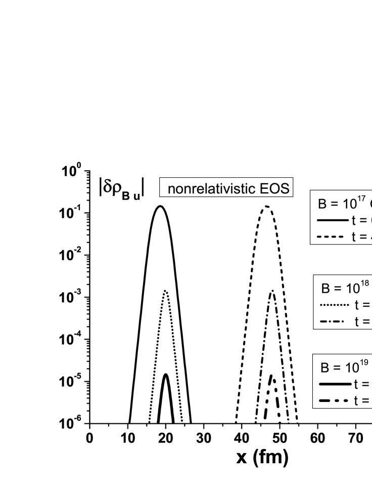
Figure 1: Nonrelativistic EOS: solitonic behavior of $|{{\delta\rho_{B}}_{u}}|$ for several times and magnetic field intensities.

In Fig. 2 we show the results obtained with the mQCD EOS for the parameters $B_{QCD}=70\,MeV/fm^{3}$, $g_{h}=0.05$, $m_{G}=300\,MeV$, $\xi_{0}=20\,fm$, $\lambda=1\,fm^{-1}$ and $\gamma=0.1$ . The common chemical potential for all quarks is $\nu_{f}=300\,MeV$ and for the chosen values of the magnetic field we have background densities $\rho_{0}=2\rho_{N}\sim 2.1\rho_{N}$ $(B=10^{17}\,G\sim 10^{19}\,G)$, which, with the use of (27) lead to ${c_{s\,\perp}}\cong 0.2$ . The propagation speed of the pulse is $\alpha+\gamma=0.5$ , which does not violate causality.

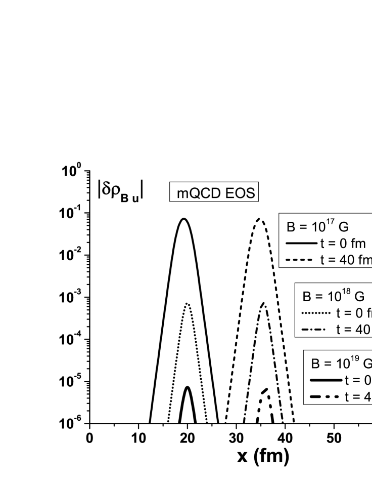
Figure 2: mQCD EOS: solitonic behavior of $|{{\delta\rho_{B}}_{u}}|$ for several times and magnetic field intensities.

Similar behavior is found when $|{{\delta\rho_{B}}_{u}}|$ is plotted as a function of the $y$ coordinate (perpendicular to the magnetic field) and of the $z$ coordinate (along the magnetic field).

VI Conclusions

In this work we focused on nonlinear wave propagation in a cold and magnetized quark gluon plasma. Including the effects of a strong magnetic field both in the equation of state and in the basic equations of hydrodynamics, we derived from the latter a wave equation for a perturbation in the baryon density. This wave equation could be identified as the reduced Ostrovsky equation (ROE), which has a known analytical solution given by a rarefaction solitonic pulse of the baryon perturbation. The numerical analysis and a possible phenomenological application in the context of heavy ion collisions or in compact stars will be investigated in a future work. At a qualitative level we can observe that the most remarkable effect of the magnetic field, as can be seen in the coefficient $\Gamma$ by (31), is to reduce the wave amplitude. We therefore corroborate and extend the conclusion found in azam .

VII Appendix

To establish the integrability of (30), we employ the change of variables developed in roe :

$$\xi=\Omega+\beta\int_{-\infty}^{\eta}\psi(\Omega,\eta^{\prime})d\eta^{\prime}\,+\alpha\,\eta+\xi_{0}\hskip 11.38092pt\textrm{,}\hskip 17.07182ptt=\eta\hskip 17.07182pt\textrm{and}\hskip 17.07182pt{\delta\rho_{B}}_{f}(\xi,t)=\psi(\Omega,\eta)$$ (35)

where $\xi_{0}$ is an arbitrary constant. From (35) we have the operators:

$${\frac{\partial}{\partial\xi}}={\frac{1}{h(\Omega,\eta)}}{\frac{\partial}{\partial\Omega}}\hskip 17.07182pt\textrm{and}\hskip 17.07182pt{\frac{\partial}{\partial t}}={\frac{\partial}{\partial\eta}}-{\frac{\beta}{h(\Omega,\eta)}}\,\psi{\frac{\partial}{\partial\Omega}}-{\frac{\alpha}{h(\Omega,\eta)}}\,{\frac{\partial}{\partial\Omega}}$$ (36)

where the function $h(\Omega,\eta)$ is given by:

$$h(\Omega,\eta)=1+\beta\int_{-\infty}^{\eta}\Big{[}{\frac{\partial}{\partial\Omega}}\psi(\Omega,\eta^{\prime})\Big{]}\,\,d\eta^{\prime}$$ (37)

The equation (30) rewritten in terms of (36) and (37) is:

$$h(\Omega,\eta)={\frac{1}{\Gamma\,\psi}}{\frac{\partial}{\partial\Omega}}{\frac{\partial\psi}{\partial\eta}}$$ (38)

From (37) we have:

$${\frac{\partial h}{\partial\eta}}=\beta\,{\frac{\partial\psi}{\partial\Omega}}$$ (39)

Finally, inserting (38) in (39) we arrive at the following equation:

$$\psi\,{\frac{\partial^{2}}{\partial\eta^{2}}}\,{\frac{\partial\psi}{\partial\Omega}}-{\frac{\partial\psi}{\partial\eta}}{\frac{\partial}{\partial\Omega}}{\frac{\partial\psi}{\partial\eta}}-(\beta\Gamma)(\psi)^{2}\,{\frac{\partial\psi}{\partial\Omega}}=0$$ (40)

which is the ROE equation (30) rewritten in a integrable form. To solve (40) we apply the hyperbolic tangent function method as described in w2 ; weset ; tangh and find the following exact solutions:

$$\psi_{I}(\Omega,\eta)=-{\frac{6\gamma^{2}\lambda^{2}}{\beta\Gamma}}sech^{2}\Big{[}\lambda(\Omega-\gamma\eta)\Big{]}\hskip 19.91684pt\textrm{or}\hskip 19.91684pt\psi_{II}(\Omega,\eta)={\frac{4\gamma^{2}\lambda^{2}}{\beta\Gamma}}+\psi_{I}(\Omega,\eta)$$ (41)

The parameters $\lambda$, which is the inverse of the width and $\gamma$, the speed, are integration constants and are free to be chosen. The negative sign in the $-sech^{2}[\dots]$ function in (41) describes a rarefaction pulse. Such negative sign is due the condition $(\alpha\Gamma)>0$.

Considering $\psi_{I}$ from (41) in (35) we obtain the following parametric solution of (30):

$${{\delta\rho_{B}}_{f}}(\xi,t)=-{\frac{6\gamma^{2}\lambda^{2}}{\beta\Gamma}}sech^{2}\Big{[}\lambda\Big{(}\Omega-\gamma t\Big{)}\Big{]}$$ (42)

with

$$\xi=\Omega+\alpha\,t+\xi_{0}+{\frac{6\gamma\lambda}{\beta\Gamma}}\Big{\{}tanh\Big{[}\lambda\Big{(}\Omega-\gamma t\Big{)}\Big{]}-1\Big{\}}$$ (43)

As previously mentioned, the last two expressions are (33) and (34), respectively.

We do not consider $\psi_{II}$ of (41) as solution of (30). The reason is to avoid the divergence due the constant term of $\psi_{II}$ in the integral present in (35):

$$\beta\int_{-\infty}^{\eta}{\frac{4\gamma^{2}\lambda^{2}}{\beta\Gamma}}\,d\eta^{\prime}\rightarrow\infty$$

References

• (1) See for example, the recent brief review articles and references therein: J. Schukraft, arXiv:1705.02646; V. Greco, J. Phys. Conf. Ser. 779, 012022 (2017).
• (2) P. Braun-Munzinger, V. Koch, T. Schaefer and J. Stachel, Phys. Rept. 621, 76 (2016).
• (3) E. J. Ferrer, arXiv:1703.09270 and references therein.
• (4) A. Rafiei and K. Javidan, Phys. Rev. C 94, 034904 (2016); S. Shi, J. Liao and P. Zhuang, Phys. Rev. C 90, 064912 (2014); E. Shuryak and P. Staig, Phys. Rev. C 88, 064905 (2013); Phys. Rev. C 88, 054903 (2013) P. Staig and E. Shuryak, Phys. Rev. C 84, 044912 (2011); Phys. Rev. C 84, 034908 (2011).
• (5) C. Plumberg and J. I. Kapusta, Phys. Rev. C 95, 044910 (2017); M. Nahrgang, M. Bluhm, T. Schaefer and S. Bass, arXiv:1704.03553; G. Wilk and Z. Wlodarczyk, arXiv:1701.06401; Y. Akamatsu, A. Mazeliauskas and D. Teaney, Phys. Rev. C 95, 014909 (2017); J. I. Kapusta, B. Müller and M. Stephanov, Phys. Rev. C 85, 054906 (2012).
• (6) H. Washimi and T. Taniuti, Phys. Rev. Lett. 17, 996 (1966); R.C. Davidson, “Methods in Nonlinear Plasma Theory”, Academic Press, New York an London, (1972); H. Leblond, J. Phys. B: At. Mol. Opt. Phys. 41, 043001 (2008).
• (7) D. A. Fogaça, F. S. Navarra and L. G. Ferreira Filho, in Williams, Matthew C.: Solitons: Interactions, Theoretical and Experimental Challenges and Perspectives, 191-256 [arXiv:1212.6932 [nucl-th]], ISBN:-978-1-62618-234-9;
• (8) D. A. Fogaça, F. S. Navarra, L. G. Ferreira Filho, Comm. Nonlin. Sci. Num. Sim. 18, 221 (2013); D. A. Fogaça, H. Marrochio, F. S. Navarra and J. Noronha, Nucl. Phys. A 934, 18 (2015).
• (9) J. D. Anand, S. N. Biswas and M. Kumar, Prog. Theor. Phys.  62, 568 (1979).
• (10) D. E. Kharzeev, L. D. McLerran and H. J. Warringa, Nucl. Phys. A 803, 227 (2008); V. Skokov, A. Y. Illarionov and V. Toneev, Int. J. Mod. Phys. A 24, 5925 (2009).
• (11) D. A. Fogaça, S. M. Sanches Jr. and F. S. Navarra, Nucl. Phys. A 973, 48 (2018).
• (12) T. Ablyazimov et al. [CBM Collaboration], Eur. Phys. J. A 53, 60 (2017); B. Friman, C. Hohne, J. Knoll, S. Leupold, J. Randrup, R. Rapp and P. Senger, Lect. Notes Phys. 814, 1 (2011).
• (13) theor.jinr.ru/twiki-cgi/view/NICA/NICAWhitePaper; see also: K. A. Bugaev, arXiv:0909.0731 [nucl-th] and references therein.
• (14) A. Ghaani, K. Javidan and M. Sarbishaei, Astrophys. Space Sci. 358, 20 (2015).
• (15) A. Ghaani and K. Javidan, arXiv:1712.10298 [hep-th].
• (16) L. Landau and E. Lifchitz, “Fluid Mechanics”, Pergamon Press, Oxford, (1987).
• (17) N. K. Glendenning, “Compact stars”, Springer-Verlag, New York, 2000.
• (18) D. Martínez-Gómez, R. Soler and J. Terradas, APJ 832, 101 (2016); APJ 837, 80 (2017).
• (19) C. Patrignani et al. [Particle Data Group], Chin. Phys. C 40, 100001 (2016). See also: http://pdg.lbl.gov/2017/tables/rpp2017-sum-quarks.pdf.
• (20) D. A. Fogaça, S. M. Sanches, T. F. Motta and F. S. Navarra, Phys. Rev. C 94, 055805 (2016).
• (21) G. Kowal, D. A. Falceta-Goncalves and A. Lazarian, New J. Phys. 13, 053001 (2011); M. S. Nakwacki, E. M. d. Gouveia Dal Pino, G. Kowal and R. Santos-Lima, J. Phys. Conf. Ser.  370, 012043 (2012).
• (22) D. A. Fogaça and F. S. Navarra, Phys. Lett. B 700, 236 (2011).
• (23) V. O. Vakhnenko, E. J. Parkes, Nonlinearity 11, 1457 (1998); Y. A. Stepanyants, Chaos Solitons Fractals 28, 193 (2006); E. Yusufo$\breve{g}$lu , A. Bekir, Applied Mathematics and Computation 186, 256 (2007); E. J. Parkers, Chaos Solitons Fractals 31, 602 (2007); E. R. Johnson, R. H. J. Grimshaw, Phys. Rev. E 88, 021201 (2013); R. G., D. Pelinovsky, Discrete and Continuous Dynamical Systems, 34, 557 (2014) [arXiv:1210.6526v2]; R. Grimshaw, D. Pelinovsky, Discrete and Continuous Dynamical Systems, 34, 557 (2014) [arXiv:1210.6526v2]; Bao-Feng Feng, Ken-ichi Maruno and Yasuhiro Ohta, Journal of Physics A: Mathematical and Theoretical, 50, 055201 (2017).
• (24) L. A. Ostrovsky, Oceanology 18, 119 (1978).
• (25) M. A. Hoefer, M. J. Ablowitz, I. Coddington, E. A. Cornell, P. Engels and V. Schweikhard, Phys. Rev. A 74, 023623 (2006); T.S. El-Danaf and M.A. Ramadan, Open Appl. Math. J. I, 1 (2007); M. Kulkarni and A.G. Abanov, Phys. Rev. A 86, 033614 (2012).