Positivity-Preserving Analysis of Numerical Schemes for Ideal Magnetohydrodynamics

Abstract

Numerical schemes provably preserving the positivity of density and pressure are highly desirable for ideal magnetohydrodynamics (MHD), but the rigorous positivity-preserving (PP) analysis remains challenging. The difficulties mainly arise from the intrinsic complexity of the MHD equations as well as the indeterminate relation between the PP property and the divergence-free condition on the magnetic field. This paper presents the first rigorous PP analysis of conservative schemes with the Lax-Friedrichs (LF) flux for one- and multi-dimensional ideal MHD. The significant innovation is the discovery of the theoretical connection between the PP property and a discrete divergence-free (DDF) condition. This connection is established through the generalized LF splitting properties, which are alternatives of the usually-expected LF splitting property that does not hold for ideal MHD. The generalized LF splitting properties involve a number of admissible states strongly coupled by the DDF condition, making their derivation very difficult. We derive these properties via a novel equivalent form of the admissible state set and an important inequality, which is skillfully constructed by technical estimates. Rigorous PP analysis is then presented for finite volume and discontinuous Galerkin schemes with the LF flux on uniform Cartesian meshes. In the 1D case, the PP property is proved for the first-order scheme with proper numerical viscosity, and also for arbitrarily high-order schemes under conditions accessible by a PP limiter. In the 2D case, we show that the DDF condition is necessary and crucial for achieving the PP property. It is observed that even slightly violating the proposed DDF condition may cause failure to preserve the positivity of pressure. We prove that the 2D LF type scheme with proper numerical viscosity preserves both the positivity and the DDF condition. Sufficient conditions are derived for 2D PP high-order schemes, and extension to 3D is discussed. Numerical examples further confirm the theoretical findings.

65M60, 65M08, 65M12, 35L65, 76W05

1 Introduction

Magnetohydrodynamics (MHD) play an important role in many fields including astrophysics, space physics and plasma physics, etc. The $d$-dimensional ideal compressible MHD equations can be written as

(1) $$\frac{{\partial{\bf U}}}{{\partial t}}+\sum\limits_{i=1}^{d}{\frac{{\partial{{\bf F}_{i}}({\bf U})}}{{\partial x_{i}}}}={\bf 0},$$

together with the divergence-free condition on the magnetic field ${\bf B}=(B_{1},B_{2},B_{3})$,

(2) $$\sum\limits_{i=1}^{d}\frac{\partial B_{i}}{\partial x_{i}}=0,$$

where $d=1,2$ or $3$. In (1), the conservative vector ${\bf U}=(\rho,\rho{\bf v},{\bf B},E)^{\top}$, and ${\bf F}_{i}({\bf U})$ denotes the flux in the $x_{i}$-direction, $i=1,\cdots,d$, defined by

$${\bf F}_{i}({\bf U})=\Big{(}\rho v_{i},~{}\rho v_{i}{\bf v}-B_{i}{\bf B}+p_{tot}{\bf e}_{i},~{}v_{i}{\bf B}-B_{i}{\bf v},~{}v_{i}(E+p_{tot})-B_{i}({\bf v}\cdot{\bf B})\Big{)}^{\top}.$$

Here $\rho$ is the density, the vector ${\bf v}=(v_{1},v_{2},v_{3})$ denotes the fluid velocity, $p_{\rm tot}$ is the total pressure consisting of the gas pressure $p$ and magnetic pressure $p_{m}=\frac{|{\bf B}|^{2}}{2}$, the vector ${\bf e}_{i}$ represents the $i$-th row of the unit matrix of size 3, and $E=\rho e+\frac{1}{2}\left(\rho|{\bf v}|^{2}+|{\bf B}|^{2}\right)$ is the total energy consisting of thermal, kinetic and magnetic energies with $e$ denoting the specific internal energy. The equation of state (EOS) is needed to close the system (1)–(2). For ideal gases it is given by

(3) $$p=(\gamma-1)\rho e,$$

where the adiabatic index $\gamma>1$ . Although (3) is widely used, there are situations where it is more appropriate to use other EOS. A general EOS can be expressed as

(4) $$p=p(\rho,e),$$

which is assumed to satisfy the following condition

(5) $$\mbox{if}\quad\rho>0,\quad\mbox{then}\quad e>0~{}\Leftrightarrow~{}p(\rho,e)>0.$$

Such condition is reasonable, holds for the ideal EOS (3) and was also used in [53].

Since (1) involves strong nonlinearity, its analytic treatment is very difficult. Numerical simulation is a primary approach to explore the physical mechanisms in MHD. In the past few decades, the numerical study of MHD has attracted much attention, and various numerical schemes have been developed for (1). Besides the standard difficulty in solving nonlinear hyperbolic conservation laws, an additional numerical challenge for the MHD system comes from the divergence-free condition (2). Although (2) holds for the exact solution as long as it does initially, it cannot be easily preserved by a numerical scheme (for $d\geq 2$). Numerical evidence and some analysis in the literature indicate that negligence in dealing with the condition (2) can lead to numerical instabilities or nonphysical features in the computed solutions, see e.g., [9, 16, 6, 38, 15, 24]. Up to now, many numerical techniques have been proposed to control the divergence error of numerical magnetic field. They include but are not limited to: the eight-wave methods [32, 10], the projection method [9], the hyperbolic divergence cleaning methods [15], the locally divergence-free methods [24, 49], the constrained transport method [16] and its many variants [35, 6, 29, 2, 30, 37, 36, 34, 1, 27, 3, 26, 25, 14]. The readers are also referred to an early survey in [38].

Another numerical challenge in the simulation of MHD is preserving the positivity of density $\rho$ and pressure $p$. In physics, these two quantities are non-negative. Numerically their positivity is very critical, but not always satisfied by numerical solutions. In fact, once the negative density or pressure is obtained in the simulations, the discrete problem will become ill-posed due to the loss of hyperbolicity, causing the break-down of the simulation codes. However, most of the existing MHD schemes are generally not positivity-preserving (PP), and thus may suffer from a large risk of failure when simulating MHD problems with strong discontinuity, low density, low pressure or low plasma-beta. Several efforts have been made to reduce such risk. Balsara and Spicer [5] proposed a strategy to maintain positive pressure by switching the Riemann solvers for different wave situations. Janhunen [22] designed a new 1D Riemann solver for the modified MHD system, and claimed its PP property by numerical experiments. Waagan [39] designed a positive linear reconstruction for second-order MUSCL-Hancock scheme, and conducted some 1D analysis based on the presumed PP property of the first-order scheme. From a relaxation system, Bouchut et al. [7, 8] derived a multiwave approximate Riemann solver for 1D ideal MHD, and deduced sufficient conditions for the solver to satisfy discrete entropy inequalities and the PP property. Recent years have witnessed some significant advances in developing bound-preserving high-order schemes for hyperbolic systems (e.g., [50, 51, 52, 21, 47, 28, 42, 31, 44, 48]). High-order limiting techniques were well developed in [4, 11] for the finite volume or DG methods of MHD, to enforce the admissibility of the reconstructed or DG polynomial solutions at certain nodal points. These techniques are based on a presumed proposition that the cell-averaged solutions computed by those schemes are always admissible. Such proposition has not yet been rigorously proved for those methods, although it could be deduced for the 1D schemes in [11] under some assumptions (see Remark 2.18). With the presumed PP property of the Lax-Friedrichs (LF) scheme, Christlieb et al. [13, 12] developed PP high-order finite difference methods for (1) by extending the parametrized flux limiters [47, 46].

It was demonstrated numerically that the above PP treatments could enhance the robustness of MHD codes. However, as mentioned in [13], there was no rigorous proof to genuinely and completely show the PP property of those or any other schemes for (1) in the multi-dimensional cases. Even for the simplest first-order schemes, such as the LF scheme, the PP property is still unclear in theory. Moreover, it is also unanswered theoretically whether the divergence-free condition (2) is connected with the PP property of schemes for (1). Therefore, it is significant to explore provably PP schemes for (1) and develop related theories for rigorous PP analysis.

The aim of this paper is to carry out a rigorous PP analysis of conservative finite volume and DG schemes with the LF flux for one- and multi-dimensional ideal MHD system (1). Such analysis is extremely nontrivial and technical. The challenges mainly come from the intrinsic complexity of the system (1)–(2), as well as the unclear relation between the PP property and the divergence-free condition on the magnetic field. Fortunately, we find an important novel starting point of the analysis, based on an equivalent form of the admissible state set. This form helps us to successfully derive the generalized LF splitting properties, which couple a discrete divergence-free (DDF) condition for the magnetic field with the convex combination of some LF splitting terms. These properties imply a theoretical connection between the PP property and the proposed DDF condition. As the generalized LF splitting properties involve a number of strongly coupled states, their discovery and proofs are extremely technical. With the aid of these properties, we present the rigorous PP analysis for finite volume and DG schemes on uniform Cartesian meshes. Meanwhile, our analysis also reveals that the DDF condition is necessary and crucial for achieving the PP property. This finding is consistent with the existing numerical evidences that violating the divergence-free condition may more easily cause negative pressure (see e.g., [9, 2, 34, 4]), as well as our previous work on the relativistic MHD [43]. Without considering the relativistic effect, the system (1) yields unboundedness of velocities and poses difficulties essentially different from the relativistic case. It is also worth mentioning that, as it will be shown, the 1D LF scheme is not always PP for piecewise constant $B_{1}$, making some existing techniques [50] for PP analysis inapplicable in the multi-dimensional ideal MHD case. Contrary to the usual expectation, we also find that the 1D LF scheme with a standard numerical viscosity parameter is not always PP, no matter how small the CFL number is. A proper viscosity parameter should be estimated, introducing additional difficulties in the analysis. Note that, for the incompressible flow system in the vorticity-stream function formulation, there is also a divergence-free condition (but) on fluid velocity, i.e., the incompressibility condition, which is crucial in designing schemes that satisfies the maximum principle of vorticity, see e.g. [50]. An important difference in our MHD case is that our divergence-free quantity (the magnetic field) is also nonlinearly related to defining the concerned positive quantity — the internal energy or pressure, see (6).

The paper is organized as follows. Section 2 gives several important properties of the admissible states for the PP analysis. Sections 3 and 4 respectively study 1D and 2D PP schemes. Numerical verifications are provided in Section 5, and the 3D extension are given in Appendix B. Section 6 concludes the paper with several remarks.

2 Admissible states

Under the condition (5), it is natural to define the set of admissible states $\bf U$ of the ideal MHD as follows.

Definition 2.1.

The set of admissible states of the ideal MHD is defined by

(6) $${\mathcal{G}}=\left\{{\bf U}=(\rho,{\bf m},{\bf B},E)^{\top}~{}\Big{|}~{}\rho>0,~{}{\mathcal{E}}({\bf U}):=E-\frac{1}{2}\left(\frac{|{\bf m}|^{2}}{\rho}+|{\bf B}|^{2}\right)>0\right\},$$

where ${\mathcal{E}}({\bf U})=\rho e$ denotes the internal energy.

Given that the initial data are admissible, a scheme is defined to be PP if the numerical solutions always stay in the set $\mathcal{G}$. One can see from (6) that it is difficult to numerically preserve the positivity of ${\mathcal{E}}$, whose computation nonlinearly involves all the conservative variables. In most of numerical methods, the conservative quantities are themselves evolved according to their own conservation laws, which are seemingly unrelated to and numerically do not necessarily guarantee the positivity of the computed ${\mathcal{E}}$. In theory, it is indeed a challenge to make a priori judgment on whether a scheme is always PP under all circumstances or not.

2.1 Basic properties

To overcome the difficulties arising from the nonlinearity of the function ${\mathcal{E}}({\bf U})$, we propose the following equivalent definition of ${\mathcal{G}}$.

Lemma 2.2 (Equivalent definition).

The admissible state set ${\mathcal{G}}$ is equivalent to

(7) $${\mathcal{G}}_{*}=\left\{{\bf U}=(\rho,{\bf m},{\bf B},E)^{\top}~{}\Big{|}~{}\rho>0,~{}~{}~{}{\bf U}\cdot{\bf n}^{*}+\frac{|{\bf B}^{*}|^{2}}{2}>0,~{}\forall~{}{\bf v}^{*},{\bf B}^{*}\in{\mathbb{R}}^{3}\right\},$$

where

$${\bf n}^{*}=\bigg{(}\frac{|{\bf v}^{*}|^{2}}{2},~{}-{\bf v}^{*},~{}-{\bf B}^{*},~{}1\bigg{)}^{\top}.$$

Proof 2.3.

If ${\bf U}\in{\mathcal{G}}$, then $\rho>0$, and for any ${\bf v}^{*},{\bf B}^{*}\in{\mathbb{R}}^{3}$,

$${\bf U}\cdot{\bf n}^{*}+\frac{|{\bf B}^{*}|^{2}}{2}=\frac{\rho}{2}\big{|}\rho^{-1}{\bf m}-{\bf v}^{*}\big{|}^{2}+\frac{|{\bf B}-{\bf B}^{*}|^{2}}{2}+{\mathcal{E}}({\bf U})\geq{\mathcal{E}}({\bf U})>0,$$

that is ${\bf U}\in{\mathcal{G}}_{*}$. Hence ${\mathcal{G}}\subset{\mathcal{G}}_{*}$. On the other hand, if ${\bf U}\in{\mathcal{G}}_{*}$, then $\rho>0$, and taking ${\bf v}^{*}=\rho^{-1}{\bf m}$ and ${\bf B}^{*}={\bf B}$ gives $0<{\bf U}\cdot{\bf n}^{*}+{|{\bf B}^{*}|^{2}}/{2}={\mathcal{E}}({\bf U}).$ This means ${\bf U}\in{\mathcal{G}}$. Therefore ${\mathcal{G}}_{*}\subset{\mathcal{G}}$. In conclusion, ${\mathcal{G}}={\mathcal{G}}_{*}$.

The two constraints in (7) are both linear with respect to $\bf U$, making it more effective to analytically verify the PP property of numerical schemes for ideal MHD.

The convexity of admissible state set is very useful in bound-preserving analysis, because it can help reduce the complexity of analysis if the schemes can be rewritten into certain convex combinations, see e.g., [51, 53, 40]. For the ideal MHD, the convexity of $\mathcal{G}_{*}$ or $\mathcal{G}$ can be easily shown by definition.

Lemma 2.4 (Convexity).

The set ${\mathcal{G}}_{*}$ is convex. Moreover, $\lambda{\bf U}_{1}+(1-\lambda){\bf U}_{0}\in{\mathcal{G}}_{*}$ for any ${\bf U}_{1}\in{\mathcal{G}}_{*},{\bf U}_{0}\in\overline{\mathcal{G}}_{*}$ and $\lambda\in(0,1]$, where $\overline{\mathcal{G}}_{*}$ is the closure of ${\mathcal{G}}_{*}$.

Proof 2.5.

The first component of ${\bf U}_{\lambda}:=\lambda{\bf U}_{1}+(1-\lambda){\bf U}_{0}$ equals $\lambda\rho_{1}+(1-\lambda)\rho_{0}>0$. For $\forall~{}{\bf v}^{*},{\bf B}^{*}\in{\mathbb{R}}^{3}$, ${\bf U}_{\lambda}\cdot{\bf n}^{*}+\frac{|{\bf B}^{*}|^{2}}{2}=\lambda\big{(}{\bf U}_{1}\cdot{\bf n}^{*}+\frac{|{\bf B}^{*}|^{2}}{2}\big{)}+(1-\lambda)\big{(}{\bf U}_{0}\cdot{\bf n}^{*}+\frac{|{\bf B}^{*}|^{2}}{2}\big{)}>0.$ This shows ${\bf U}_{\lambda}\in{\mathcal{G}}_{*}$. The proof is completed by the definition of convexity.

We also have the following orthogonal invariance, which can be verified directly.

Lemma 2.6 (Orthogonal invariance).

Let ${\bf T}:={\rm diag}\{1,{\bf T}_{3},{\bf T}_{3},1\}$, where ${\bf T}_{3}$ is any orthogonal matrix of size 3. If ${\bf U}\in{\mathcal{G}}$, then ${\bf T}{\bf U}\in{\mathcal{G}}$.

We refer to the following property (8) as the LF splitting property,

(8) $${\bf U}\pm\frac{{\bf F}_{i}({\bf U})}{\alpha}\in{\mathcal{G}},\quad\forall~{}{\bf U}\in{\mathcal{G}},~{}\forall~{}\alpha\geq\chi{\mathscr{R}}_{i}({\bf U}),$$

where $\chi\geq 1$ is some constant, and ${\mathscr{R}}_{i}({\bf U})$ is the spectral radius of the Jacobian matrix in $x_{i}$-direction, $i=1,2,3$. For the ideal MHD system with the EOS (4), one has [32]

$${\mathscr{R}}_{i}({\bf U})=|v_{i}|+\mathcal{C}_{i},$$

with

$${\mathcal{C}}_{i}:=\frac{1}{\sqrt{2}}\left[\mathcal{C}_{s}^{2}+\frac{|{\bf B}|^{2}}{\rho}+\sqrt{\left(\mathcal{C}_{s}^{2}+\frac{|{\bf B}|^{2}}{\rho}\right)^{2}-4\frac{\mathcal{C}_{s}^{2}B_{i}^{2}}{\rho}}\right]^{\frac{1}{2}},$$

where $\mathcal{C}_{s}=\sqrt{\gamma p/\rho}$ is the sound speed.

If true, the LF splitting property would be very useful in analyzing the PP property of the schemes with the LF flux, see its roles in [51, 42, 40] for the equations of hydrodynamics. Unfortunately, for the ideal MHD, (8) is untrue in general, as evidenced numerically in [11] for ideal gases. In fact, one can disprove (8), see the proof of the following proposition in Appendix A.1.

Proposition 2.7.

The LF splitting property (8) does not hold in general.

2.2 Generalized LF splitting properties

Since (8) does not hold, we would like to seek some alternative properties which are weaker than (8). By considering the convex combination of some LF splitting terms, we discover the generalized LF splitting properties under some “discrete divergence-free” condition for the magnetic field. As one of the most highlighted points of this paper, the discovery and proofs of such properties are very nontrivial and extremely technical.

2.2.1 A constructive inequality

We first construct an inequality, which will play a pivotal role in establishing the generalized LF splitting properties.

Lemma 2.8.

If ${\bf U},\tilde{\bf U}\in{\mathcal{G}}$, then the inequality

(9) $$\bigg{(}{\bf U}-\frac{{\bf F}_{i}({\bf U})}{\alpha}+\tilde{\bf U}+\frac{{\bf F}_{i}(\tilde{\bf U})}{\alpha}\bigg{)}\cdot{\bf n}^{*}+|{\bf B}^{*}|^{2}+\frac{B_{i}-\tilde{B}_{i}}{\alpha}({\bf v}^{*}\cdot{\bf B}^{*})>0,$$

holds for any ${\bf v}^{*},{\bf B}^{*}\in{\mathbb{R}}^{3}$ and $|\alpha|>\alpha_{i}({\bf U},\tilde{\bf U})$, where $i\in\{1,2,3\}$, and

(10) $$\alpha_{i}({\bf U},\tilde{\bf U})=\min_{\sigma\in\mathbb{R}}\alpha_{i}({\bf U},\tilde{\bf U};\sigma),$$

$$\alpha_{i}({\bf U},\tilde{\bf U};\sigma)=\max\big{\{}|v_{i}|+{\mathscr{C}}_{i},|\tilde{v}_{i}|+\tilde{\mathscr{C}}_{i},|\sigma v_{i}+(1-\sigma)\tilde{v}_{i}|+\max\{{\mathscr{C}}_{i},\tilde{\mathscr{C}}_{i}\}\big{\}}+f({\bf U},\tilde{\bf U};\sigma),$$

with

$$f({\bf U},\tilde{\bf U};\sigma)=\frac{|\tilde{\bf B}-{\bf B}|}{\sqrt{2}}\sqrt{\frac{\sigma^{2}}{\rho}+\frac{(1-\sigma)^{2}}{\tilde{\rho}}},$$

$${\mathscr{C}}_{i}=\frac{1}{\sqrt{2}}\left[{\mathscr{C}}_{s}^{2}+\frac{|{\bf B}|^{2}}{\rho}+\sqrt{\left({\mathscr{C}}_{s}^{2}+\frac{|{\bf B}|^{2}}{\rho}\right)^{2}-4\frac{{\mathscr{C}}_{s}^{2}B_{i}^{2}}{\rho}}\right]^{\frac{1}{2}},$$

and ${\mathscr{C}}_{s}=\frac{p}{\rho\sqrt{2e}}$.

Proof 2.9.

(i). We first prove (9) for $i=1$. Let define

$$\Pi_{u}=\big{(}{\bf U}+\tilde{\bf U}\big{)}\cdot{\bf n}^{*}+|{\bf B}^{*}|^{2},\quad\Pi_{f}=\big{(}{\bf F}_{1}({\bf U})-{\bf F}_{1}(\tilde{\bf U})\big{)}\cdot{\bf n}^{*}-\big{(}B_{1}-\tilde{B}_{1}\big{)}({\bf v}^{*}\cdot{\bf B}^{*}).$$

Then it only needs to show

(11) $$\frac{|\Pi_{f}|}{\Pi_{u}}\leq\alpha_{1}({\bf U},\tilde{\bf U}),$$

by noting that

(12) $$\Pi_{u}=|{\bm{\theta}}|^{2}>0,$$

where the nonzero vector ${\bm{\theta}}\in{\mathbb{R}}^{14}$ is defined as

$${\bm{\theta}}=\frac{1}{\sqrt{2}}\Big{(}\sqrt{\rho}({\bf v}-{\bf v}^{*}),~{}{\bf B}-{\bf B}^{*},~{}\sqrt{2\rho e},~{}\sqrt{\tilde{\rho}}(\tilde{\bf v}-{\bf v}^{*}),~{}\tilde{\bf B}-{\bf B}^{*},~{}\sqrt{2\tilde{\rho}\tilde{e}}\Big{)}^{\top}.$$

The proof of (11) is divided into the following two steps.

Step 1. Reformulate $\Pi_{f}$ into a quadratic form in the variables $\theta_{j},1\leq j\leq 14$. We require that the coefficients of the quadratic form do not depends on ${\bf v}^{*}$ and ${\bf B}^{*}$. This is very nontrivial and becomes the key step of the proof. We first arrange $\Pi_{f}$ by a technical decomposition

(13) $$\Pi_{f}=\Pi_{1}+\Pi_{2}+\Pi_{3}+(\Pi_{4}-\tilde{\Pi}_{4}),$$

where

$$\Pi_{j}=\frac{1}{2}v_{1}^{*}\big{(}B_{j}^{2}-\tilde{B}_{j}^{2}\big{)}-v_{1}^{*}B_{j}^{*}(B_{j}-\tilde{B}_{j}),\quad j=1,2,3,$$

$$\Pi_{4}=\frac{\rho v_{1}}{2}|{\bf v}-{\bf v}^{*}|^{2}+v_{1}\rho e+p(v_{1}-v_{1}^{*})+\sum_{j=2}^{3}(B_{j}(v_{1}-v_{1}^{*})-B_{1}(v_{j}-v_{j}^{*}))(B_{j}-B_{j}^{*}),$$

$$\tilde{\Pi}_{4}=\frac{\tilde{\rho}\tilde{v}_{1}}{2}|\tilde{\bf v}-{\bf v}^{*}|^{2}+\tilde{v}_{1}\tilde{\rho}\tilde{e}+\tilde{p}(\tilde{v}_{1}-v_{1}^{*})+\sum_{j=2}^{3}(\tilde{B}_{j}(\tilde{v}_{1}-v_{1}^{*})-\tilde{B}_{1}(\tilde{v}_{j}-v_{j}^{*}))(\tilde{B}_{j}-B_{j}^{*}).$$

One can immediately rewrite $\Pi_{4}$ and $\tilde{\Pi}_{4}$ as

$$\Pi_{4}=v_{1}\Big{(}\sum_{j=1}^{3}\theta_{j}^{2}+\theta_{7}^{2}\Big{)}+2{\mathscr{C}}_{s}\theta_{1}\theta_{7}+\frac{2B_{2}}{\sqrt{\rho}}\theta_{1}\theta_{5}+\frac{2B_{3}}{\sqrt{\rho}}\theta_{1}\theta_{6}-\frac{2B_{1}}{\sqrt{\rho}}(\theta_{2}\theta_{5}+\theta_{3}\theta_{6}),$$

$$\tilde{\Pi}_{4}=\tilde{v}_{1}\Big{(}\sum_{j=8}^{10}\theta_{j}^{2}+\theta_{14}^{2}\Big{)}+2\tilde{\mathscr{C}}_{s}\theta_{8}\theta_{14}+\frac{2\tilde{B}_{2}}{\sqrt{\tilde{\rho}}}\theta_{8}\theta_{12}+\frac{2\tilde{B}_{3}}{\sqrt{\tilde{\rho}}}\theta_{8}\theta_{13}-\frac{2\tilde{B}_{1}}{\sqrt{\tilde{\rho}}}(\theta_{9}\theta_{12}+\theta_{10}\theta_{13}).$$

After a careful investigation, we find that $\Pi_{j}$, $j=1,2,3$, can be reformulated as

$$\begin{split}\Pi_{j}&=\sigma_{j}\frac{\tilde{B}_{j}-B_{j}}{\sqrt{\rho}}(\theta_{1}\theta_{j+3}+\theta_{1}\theta_{j+10})+(1-\sigma_{j})\frac{\tilde{B}_{j}-B_{j}}{\sqrt{\tilde{\rho}}}(\theta_{8}\theta_{j+3}+\theta_{8}\theta_{j+10})\\ &\quad+\big{(}\sigma_{j}v_{1}+(1-\sigma_{j})\tilde{v}_{1}\big{)}\theta_{j+3}^{2}-\big{(}\sigma_{j}v_{1}+(1-\sigma_{j})\tilde{v}_{1}\big{)}\theta_{j+10}^{2},\end{split}$$

where $\sigma_{1}$, $\sigma_{2}$ and $\sigma_{3}$ can be taken as any real numbers. In summary, we have reformulated $\Pi_{f}$ into a quadratic form in the variables $\theta_{j},1\leq j\leq 14$.

Step 2. Estimate the upper bound of $\frac{|\Pi_{f}|}{\Pi_{u}}$. There are several approaches to estimate the bound, resulting in different formulas. One sharp upper bound is the spectral radius of the symmetric matrix associated with the above quadratic form, but cannot be formulated explicitly and computed easily in practice. An explicit sharp upper bound is $\alpha_{1}({\bf U},\tilde{\bf U})$ in (10). It is estimated as follows. We first notice that

$$\Pi_{4} =v_{1}\Big{(}\sum_{j=1}^{3}\theta_{j}^{2}+\theta_{7}^{2}\Big{)}+{\bm{\vartheta}}_{6}^{\top}{\bf A}_{6}{\bm{\vartheta}}_{6},$$

where ${\bm{\vartheta}}_{6}=(\theta_{1},\theta_{2},\theta_{3},\theta_{5},\theta_{6},\theta_{7})^{\top}$, and

$${\bf A}_{6}=\begin{pmatrix}0&0&0&B_{2}\rho^{-\frac{1}{2}}&B_{3}\rho^{-\frac{1}{2}}&{\mathscr{C}}_{s}\\ 0&0&0&-B_{1}\rho^{-\frac{1}{2}}&0&0\\ 0&0&0&0&-B_{1}\rho^{-\frac{1}{2}}&0\\ B_{2}\rho^{-\frac{1}{2}}&-B_{1}\rho^{-\frac{1}{2}}&0&0&0&0\\ B_{3}\rho^{-\frac{1}{2}}&0&-B_{1}\rho^{-\frac{1}{2}}&0&0&0\\ {\mathscr{C}}_{s}&0&0&0&0&0\end{pmatrix}.$$

The spectral radius of ${\bf A}_{6}$ is ${\mathscr{C}}_{1}$. This gives the following estimate

(14) $$|\Pi_{4}| \leq|v_{1}|\bigg{(}\sum_{j=1}^{3}\theta_{j}^{2}+\theta_{7}^{2}\bigg{)}+|{\bm{\vartheta}}_{6}^{\top}{\bf A}_{6}{\bm{\vartheta}}_{6}|\leq|v_{1}|\bigg{(}\sum_{j=1}^{3}\theta_{j}^{2}+\theta_{7}^{2}\bigg{)}+{\mathscr{C}}_{1}|{\bm{\vartheta}}_{6}|^{2}$$

$$=(|v_{1}|+{\mathscr{C}}_{1})\bigg{(}\sum_{j=1}^{3}\theta_{j}^{2}+\theta_{7}^{2}\bigg{)}+{\mathscr{C}}_{1}\big{(}\theta_{5}^{2}+\theta_{6}^{2}\big{)}.$$

Similarly, we have

(15) $$|\tilde{\Pi}_{4}|\leq(|\tilde{v}_{1}|+\tilde{\mathscr{C}}_{1})\bigg{(}\sum_{j=8}^{10}\theta_{j}^{2}+\theta_{14}^{2}\bigg{)}+\tilde{\mathscr{C}}_{1}\big{(}\theta_{12}^{2}+\theta_{13}^{2}\big{)}.$$

Let then focus on the first three terms at the right hand of (13) and rewrite their summation as

(16) $$\Pi_{1}+\Pi_{2}+\Pi_{3}={\bm{\vartheta}}_{8}^{\top}{\bf A}_{8}{\bm{\vartheta}}_{8}+\sum_{j=1}^{3}\big{(}\sigma_{j}v_{1}+(1-\sigma_{j})\tilde{v}_{1}\big{)}\big{(}\theta_{j+3}^{2}-\theta_{j+10}^{2}\big{)},$$

where ${\bm{\vartheta}}_{8}=(\theta_{1},\theta_{4},\theta_{5},\theta_{6},\theta_{8},\theta_{11},\theta_{12},\theta_{13})^{\top}$, and

$${\bf A}_{8}=\frac{1}{2}\begin{pmatrix}~{}0~{}&~{}{\bm{\psi}}~{}&~{}0~{}&~{}{\bm{\psi}}~{}\\ ~{}{\bm{\psi}}^{\top}~{}&~{}{\bf O}~{}&~{}\tilde{\bm{\psi}}^{\top}~{}&~{}{\bf O}~{}\\ ~{}0~{}&~{}\tilde{\bm{\psi}}~{}&~{}0~{}&~{}\tilde{\bm{\psi}}~{}\\ ~{}{\bm{\psi}}^{\top}~{}&~{}{\bf O}~{}&~{}\tilde{\bm{\psi}}^{\top}~{}&~{}{\bf O}~{}\end{pmatrix},$$

with ${\bf O}$ denoting the $3\times 3$ null matrix, and

$${\bm{\psi}}=\rho^{-\frac{1}{2}}\left(\sigma_{1}(\tilde{B}_{1}-B_{1}),\sigma_{2}(\tilde{B}_{2}-B_{2}),\sigma_{3}(\tilde{B}_{3}-B_{3})\right),$$

$$\tilde{\bm{\psi}}=\tilde{\rho}^{-\frac{1}{2}}\left((1-\sigma_{1})(\tilde{B}_{1}-B_{1}),(1-\sigma_{2})(\tilde{B}_{2}-B_{2}),(1-\sigma_{3})(\tilde{B}_{3}-B_{3})\right).$$

Some algebraic manipulations show that the spectral radius of ${\bf A}_{8}$ is

$$\varrho({\bf A}_{8})=\frac{1}{2}\left[|{\bm{\psi}}|^{2}+|\tilde{\bm{\psi}}|^{2}+\sqrt{(|{\bm{\psi}}|^{2}-|\tilde{\bm{\psi}}|^{2})^{2}+4({\bm{\psi}}\cdot\tilde{\bm{\psi}})^{2}}\right]^{\frac{1}{2}}.$$

It then follows from (16) that, for $\forall\sigma_{1},\sigma_{2},\sigma_{3}\in\mathbb{R}$,

$$|\Pi_{1}+\Pi_{2}+\Pi_{3}| \leq\varrho({\bf A}_{8})|{\bm{\vartheta}}_{8}|^{2}+\sum_{j=1}^{3}\big{|}\sigma_{j}v_{1}+(1-\sigma_{j})\tilde{v}_{1}\big{|}\big{|}\theta_{j+3}^{2}-\theta_{j+10}^{2}\big{|}.$$

For simplicity, we set $\sigma_{1}=\sigma_{2}=\sigma_{3}=\sigma$, then $\varrho({\bf A}_{8})=f({\bf U},\tilde{\bf U};\sigma),$ and

$$|\Pi_{1}+\Pi_{2}+\Pi_{3}| \leq f({\bf U},\tilde{\bf U};\sigma)|{\bm{\vartheta}}_{8}|^{2}+|\sigma v_{1}+(1-\sigma)\tilde{v}_{1}|\sum_{j=1}^{3}\big{|}\theta_{j+3}^{2}-\theta_{j+10}^{2}\big{|}$$

(17) $$\leq f({\bf U},\tilde{\bf U};\sigma)|{\bm{\theta}}|^{2}+{|\sigma v_{1}+(1-\sigma)\tilde{v}_{1}|}\sum_{j=1}^{3}\big{(}\theta_{j+3}^{2}+\theta_{j+10}^{2}\big{)}.$$

Combining (13)–(15) and (17), we have

$$\begin{split}|\Pi_{f}|&\leq(|v_{1}|+{\mathscr{C}}_{1})\bigg{(}\sum_{j=1}^{3}\theta_{j}^{2}+\theta_{7}^{2}\bigg{)}+(|\tilde{v}_{1}|+\tilde{\mathscr{C}}_{1})\bigg{(}\sum_{j=8}^{10}\theta_{j}^{2}+\theta_{14}^{2}\bigg{)}+f({\bf U},\tilde{\bf U};\sigma)|{\bm{\theta}}|^{2}\\ &\quad+{\mathscr{C}}_{1}\big{(}\theta_{5}^{2}+\theta_{6}^{2}\big{)}+\tilde{\mathscr{C}}_{1}\big{(}\theta_{12}^{2}+\theta_{13}^{2}\big{)}+|\sigma v_{1}+(1-\sigma)\tilde{v}_{1}|\sum_{j=1}^{3}\big{(}\theta_{j+3}^{2}+\theta_{j+10}^{2}\big{)}\end{split}$$

$$\begin{split}&\leq(|v_{1}|+{\mathscr{C}}_{1})\bigg{(}\sum_{j=1}^{3}\theta_{j}^{2}+\theta_{7}^{2}\bigg{)}+(|\tilde{v}_{1}|+\tilde{\mathscr{C}}_{1})\bigg{(}\sum_{j=8}^{10}\theta_{j}^{2}+\theta_{14}^{2}\bigg{)}+f({\bf U},\tilde{\bf U};\sigma)|{\bm{\theta}}|^{2}\\ &\quad+\Big{(}|\sigma v_{1}+(1-\sigma)\tilde{v}_{1}|+{\mathscr{C}}_{1}\Big{)}\sum_{j=4}^{6}\theta_{j}^{2}+\Big{(}|\sigma v_{1}+(1-\sigma)\tilde{v}_{1}|+\tilde{\mathscr{C}}_{1}\Big{)}\sum_{j=11}^{13}\theta_{j}^{2}\end{split}$$

$$\begin{split}&\leq\alpha_{1}({\bf U},\tilde{\bf U};\sigma)~{}|{\bm{\theta}}|^{2}=\alpha_{1}({\bf U},\tilde{\bf U};\sigma)~{}\Pi_{u},\end{split}$$

for all $\sigma\in\mathbb{R}$. Hence

$$|\Pi_{f}|\leq\Pi_{u}\min_{\sigma\in\mathbb{R}}\alpha_{1}({\bf U},\tilde{\bf U};\sigma)=\Pi_{u}\alpha_{1}({\bf U},\tilde{\bf U}),$$

that is, the inequality (11) holds. The proof for the case of $i=1$ is completed.

(ii). We then verify the inequality (9) for the cases $i=2$ and $3$, by using the inequality (9) for the case $i=1$ as well as the orthogonal invariance in Lemma 2.6. For the case of $i=2$, we introduce an orthogonal matrix ${\bf T}={\rm diag}\{1,{\bf T}_{3},{\bf T}_{3},1\}$ with ${\bf T}_{3}:=({\bf e}_{2}^{\top},{\bf e}_{1}^{\top},{\bf e}_{3}^{\top})$, where ${\bf e}_{\ell}$ is the $\ell$-th row of the unit matrix of size 3. We then have ${\bf T}{\bf U},{\bf T}\tilde{\bf U}\in{\mathcal{G}}$ by Lemma 2.6. Let ${\mathcal{H}}_{i}({\bf U},\tilde{{\bf U}},{\bf v}^{*},{\bf B}^{*},\alpha)$ denote the left-hand side term of (9). Using (9) with $i=1$ for ${\bf T}{\bf U},{\bf T}\tilde{\bf U},{\bf v}^{*}{\bf T}_{3},{\bf B}^{*}{\bf T}_{3}$, we have

(18) $${\mathcal{H}}_{1}({\bf T}{\bf U},{\bf T}{\tilde{\bf U}},{\bf v}^{*}{\bf T}_{3},{\bf B}^{*}{\bf T}_{3},\alpha)>0,$$

for any $\alpha>\alpha_{1}({\bf T}{\bf U},{\bf T}{\tilde{\bf U}})=\alpha_{2}({\bf U},\tilde{\bf U})$. Utilizing ${\bf F}_{1}({\bf T}{\bf U})={\bf T}{\bf F}_{2}({\bf U})$ and the orthogonality of $\bf T$ and ${\bf T}_{3}$, we find that

$${\mathcal{H}}_{1}({\bf T}{\bf U},{\bf T}{\tilde{\bf U}},{\bf v}^{*}{\bf T}_{3},{\bf B}^{*}{\bf T}_{3},\alpha)={\mathcal{H}}_{2}({\bf U},\tilde{\bf U},{\bf v}^{*},{\bf B}^{*},\alpha).$$

Thus (18) implies (9) for $i=2$. Similar arguments for $i=3$. The proof is completed.

Remark 2.10.

In practice, it is not easy to determine the minimum value in (10). Since $\alpha_{i}({\bf U},\tilde{\bf U})$ only plays the role of a lower bound, one can replace it with $\alpha_{i}({\bf U},\tilde{\bf U};\sigma)$ for a special $\sigma$. For example, taking $\sigma=\frac{\rho}{\rho+\tilde{\rho}}$ minimizes $f({\bf U},\tilde{\bf U};\sigma)$ and gives

$$\alpha_{i}\bigg{(}{\bf U},\tilde{\bf U};\frac{\rho}{\rho+\tilde{\rho}}\bigg{)}=\max\bigg{\{}|v_{i}|+{\mathscr{C}}_{i},|\tilde{v}_{i}|+\tilde{\mathscr{C}}_{i},\frac{|\rho v_{i}+\tilde{\rho}\tilde{v}_{i}|}{\rho+\tilde{\rho}}+\max\{{\mathscr{C}}_{i},\tilde{\mathscr{C}}_{i}\}\bigg{\}}+\frac{|{\bf B}-\tilde{\bf B}|}{\sqrt{2(\rho+\tilde{\rho})}}.$$

Taking $\sigma=\frac{\sqrt{\rho}}{\sqrt{\rho}+\sqrt{\tilde{\rho}}}$ gives

$$\alpha_{i}\bigg{(}{\bf U},\tilde{\bf U};\frac{\sqrt{\rho}}{\sqrt{\rho}+\sqrt{\tilde{\rho}}}\bigg{)}=\max\bigg{\{}|v_{i}|+{\mathscr{C}}_{i},|\tilde{v}_{i}|+\tilde{\mathscr{C}}_{i},\frac{|\sqrt{\rho}v_{i}+\sqrt{\tilde{\rho}}\tilde{v}_{i}|}{\sqrt{\rho}+\sqrt{\tilde{\rho}}}+\max\{{\mathscr{C}}_{i},\tilde{\mathscr{C}}_{i}\}\bigg{\}}+\frac{|{\bf B}-\tilde{\bf B}|}{\sqrt{\rho}+\sqrt{\tilde{\rho}}}.$$

Let $a_{i}:=\max\{{\mathscr{R}}_{i}({\bf U}),{\mathscr{R}}_{i}(\tilde{\bf U})\}$. For the gamma-law EOS, the following proposition shows that $\alpha_{i}({\bf U},\tilde{\bf U})<2a_{i}$ and $\alpha_{i}({\bf U},\tilde{\bf U})<a_{i}+{\mathcal{O}}(|{\bf U}-\tilde{\bf U}|)$, $i=1,2,3$. When ${\bf U}=\tilde{\bf U}$ with zero magnetic field, $\alpha_{i}({\bf U},\tilde{\bf U})=|v_{i}|+\frac{p}{\rho\sqrt{2e}}$, which is consistent with the bound in the LF splitting property for the Euler equations with a general EOS [53].

Proposition 2.11.

For any admissible states ${\bf U},\tilde{\bf U}$ of an ideal gas, it holds

(19) $$\alpha_{i}({\bf U},\tilde{\bf U})<2a_{i},$$

(20) $$\alpha_{i}({\bf U},\tilde{\bf U})<a_{i}+\min\big{\{}\big{|}|v_{i}|-|\tilde{v}_{i}|\big{|},\big{|}{\mathscr{C}}_{i}-\tilde{\mathscr{C}}_{i}\big{|}\big{\}}+\frac{|{\bf B}-\tilde{\bf B}|}{\sqrt{2(\rho+\tilde{\rho})}}.$$

Proof 2.12.

The inequality (19) can be shown as follows

$$\alpha_{i}({\bf U},\tilde{\bf U}) \leq\alpha_{i}\bigg{(}{\bf U},\tilde{\bf U};\frac{\sqrt{\rho}}{\sqrt{\rho}+\sqrt{\tilde{\rho}}}\bigg{)}$$

$$\leq\max\Big{\{}|v_{i}|+{\mathscr{C}}_{i},~{}|\tilde{v}_{i}|+\tilde{\mathscr{C}}_{i}\Big{\}}+\frac{|\sqrt{\rho}v_{i}+\sqrt{\tilde{\rho}}\tilde{v}_{i}|}{\sqrt{\rho}+\sqrt{\tilde{\rho}}}+\frac{|{\bf B}-\tilde{\bf B}|}{\sqrt{\rho}+\sqrt{\tilde{\rho}}}$$

$$<a_{i}+\frac{\sqrt{\rho}}{\sqrt{\rho}+\sqrt{\tilde{\rho}}}\bigg{(}|v_{i}|+\frac{|\bf B|}{\sqrt{\rho}}\bigg{)}+\frac{\sqrt{\tilde{\rho}}}{\sqrt{\rho}+\sqrt{\tilde{\rho}}}\bigg{(}|\tilde{v}_{i}|+\frac{|\tilde{\bf B}|}{\sqrt{\tilde{\rho}}}\bigg{)}$$

$$\leq a_{i}+\max\bigg{\{}|v_{i}|+\frac{|\bf B|}{\sqrt{\rho}},|\tilde{v}_{i}|+\frac{|\tilde{\bf B}|}{\sqrt{\tilde{\rho}}}\bigg{\}}$$

$$\leq a_{i}+\max\bigg{\{}|v_{i}|+\frac{{\mathcal{C}}_{i}}{\sqrt{2}},|\tilde{v}_{i}|+\frac{|\tilde{\mathcal{C}}_{i}|}{\sqrt{2}}\bigg{\}}<2a_{i},$$

where we have used ${\mathscr{C}}_{i}<{\mathcal{C}}_{i}$ because of ${\mathscr{C}}_{s}=\sqrt{\frac{(\gamma-1)p}{2\rho}}<{\mathcal{C}}_{s}$. We then turn to prove (20). Using the triangle inequality, one can easily show that

$$|v_{i}|+\tilde{\mathscr{C}}_{i}\leq\min\big{\{}\big{|}|v_{i}|-|\tilde{v}_{i}|\big{|},\big{|}{\mathscr{C}}_{i}-\tilde{\mathscr{C}}_{i}\big{|}\big{\}}+\max\big{\{}|v_{i}|+{\mathscr{C}}_{i},|\tilde{v}_{i}|+\tilde{\mathscr{C}}_{i}\big{\}},$$

$$|\tilde{v}_{i}|+{\mathscr{C}}_{i}\leq\min\big{\{}\big{|}|v_{i}|-|\tilde{v}_{i}|\big{|},\big{|}{\mathscr{C}}_{i}-\tilde{\mathscr{C}}_{i}\big{|}\big{\}}+\max\big{\{}|v_{i}|+{\mathscr{C}}_{i},|\tilde{v}_{i}|+\tilde{\mathscr{C}}_{i}\big{\}}.$$

Therefore,

$$\max\bigg{\{}|v_{i}|+{\mathscr{C}}_{i},|\tilde{v}_{i}|+\tilde{\mathscr{C}}_{i},\frac{|\rho v_{i}+\tilde{\rho}\tilde{v}_{i}|}{\rho+\tilde{\rho}}+\max\{{\mathscr{C}}_{i},\tilde{\mathscr{C}}_{i}\}\bigg{\}}$$

$$\quad\leq\max\big{\{}|v_{i}|+{\mathscr{C}}_{i},|\tilde{v}_{i}|+\tilde{\mathscr{C}}_{i},|\tilde{v}_{i}|+{\mathscr{C}}_{i},|v_{i}|+\tilde{\mathscr{C}}_{i}\big{\}}$$

$$\quad\leq\max\big{\{}|v_{i}|+{\mathscr{C}}_{i},|\tilde{v}_{i}|+\tilde{\mathscr{C}}_{i}\big{\}}+\min\big{\{}\big{|}|v_{i}|-|\tilde{v}_{i}|\big{|},\big{|}{\mathscr{C}}_{i}-\tilde{\mathscr{C}}_{i}\big{|}\big{\}}$$

$$\quad<a_{i}+\min\big{\{}\big{|}|v_{i}|-|\tilde{v}_{i}|\big{|},\big{|}{\mathscr{C}}_{i}-\tilde{\mathscr{C}}_{i}\big{|}\big{\}}.$$

Then using $\alpha_{i}({\bf U},\tilde{\bf U})\leq\alpha_{i}\big{(}{\bf U},\tilde{\bf U};\frac{\rho}{\rho+\tilde{\rho}}\big{)}$ completes the proof.

Remark 2.13.

It is worth emphasizing the importance of the last term at the left-hand side of (9). This term is extremely technical, necessary and crucial in deriving the generalized LF splitting properties. Including this term becomes one of the breakthrough points in this paper. The value of this term is not always positive or negative. However, without this term, the inequality (9) does not hold, even if $\alpha_{i}$ is replaced with $\chi\alpha_{i}$ for any constant $\chi\geq 1$. More importantly, this term can be canceled out dexterously under the “discrete divergence-free” condition (22) or (27), see the proofs of generalized LF splitting properties in the following theorems.

Let us figure out some facts and observations. Note that the inequality (2.8) in Lemma 2.8 involves two states (${\bf U}$ and $\tilde{\bf U}$). In the relativistic MHD case (Lemma 2.9 in [43]), we derive the generalized LF splitting properties by an inequality, which is similar to (2.8) but involves only one state. It seems natural to conjecture a similar “one-state” inequality for the ideal MHD case in the following form

(21) $$\bigg{(}{\bf U}+\frac{{\bf F}_{i}({\bf U})}{\alpha}\bigg{)}\cdot{\bf n}^{*}+\frac{|{\bf B}^{*}|^{2}}{2}+\frac{1}{\alpha}\bigg{(}v_{i}^{*}\frac{|{\bf B}^{*}|^{2}}{2}-B_{i}({\bf v}^{*}\cdot{\bf B}^{*})\bigg{)}>0,\quad\forall{\bf U}\in{\mathcal{G}},~{}~{}\forall{\bf v}^{*},{\bf B}^{*}\in{\mathbb{R}}^{3},$$

for any $|\alpha|>\widehat{\alpha}_{i}({\bf U})$, where the lower bound $\widehat{\alpha}_{i}({\bf U})$ is expected to be independent of ${\bf v}^{*}$ and ${\bf B}^{*}$. For special relativistic MHD, the lower bound can be taken as the speed of light [43], which is a constant, and brings us much convenience because any velocities (e.g., $|{\bf v}|$ and $|{\bf v}^{*}|$) are uniformly smaller than such a constant according to the theory of special relativity. However, unfortunately for the ideal MHD, it is impossible to establish (21) for any $|\alpha|>\widehat{\alpha}_{i}({\bf U})$ with a desired bound $\widehat{\alpha}_{i}({\bf U})$ only dependent on ${\bf U}$. This is because the non-relativistic velocities are generally unbounded. As $v_{i}^{*}{\rm sign}(-\alpha)$ and $|{\bf B}^{*}|$ approach $+\infty$, the negative cubic term ${v_{i}^{*}|{\bf B}^{*}|^{2}}/{2\alpha}$ in (21) dominates the sign and cannot be controlled by any other terms at the left-hand side (21). Hence, the construction of generalized LF splitting properties in the ideal MHD case has difficulties essentially different from the special MHD case. If not requiring $\widehat{\alpha}_{i}$ to be independent of ${v}_{i}^{*}$, we have the following proposition with the proof displayed in Appendix A.2.

Proposition 2.14.

The inequality (21) holds for any $|\alpha|>\widehat{\alpha}_{i}({\bf U},{v}_{i}^{*})$ and any $i\in\{1,2,3\}$, where

$$\widehat{\alpha}_{i}({\bf U},{v}_{i}^{*})=\max\big{\{}|v_{i}|,|v_{i}^{*}|\big{\}}+{\mathscr{C}}_{i}.$$

2.2.2 Derivation of generalized LF splitting properties

We first present the 1D generalized LF splitting property.

Theorem 2.15 (1D generalized LF splitting).

If $\hat{\bf U}=(\hat{\rho},\hat{\bf m},\hat{\bf B},\hat{E})^{\top}$ and $\check{\bf U}=(\check{\rho},\check{\bf m},\check{\bf B},\check{E})^{\top}$ both belong to $\mathcal{G}$, and satisfy 1D “discrete divergence-free” condition

(22) $$\hat{B_{1}}-\check{B_{1}}=0,$$

then for any $\alpha>\alpha_{1}(\hat{\bf U},\check{\bf U})$ it holds

(23) $$\overline{\bf U}:=\frac{1}{2}\bigg{(}\hat{\bf U}-\frac{{\bf F}_{1}(\hat{\bf U})}{\alpha}+\check{\bf U}+\frac{{\bf F}_{1}(\check{\bf U})}{\alpha}\bigg{)}\in{\mathcal{G}}.$$

Proof 2.16.

The first component of $\overline{\bf U}$ equals $\frac{1}{2}\big{(}\hat{\rho}\big{(}1-\frac{\hat{v}_{1}}{\alpha}\big{)}+\check{\rho}\big{(}1+\frac{\check{v}_{1}}{\alpha}\big{)}\big{)}>0$. For any ${\bf v}^{*},{\bf B}^{*}\in\mathbb{R}^{3}$, utilizing Lemma 2.8 and the condition (22) gives

$$\overline{\bf U}\cdot{\bf n}^{*}+\frac{|{\bf B}^{*}|^{2}}{2}=\frac{1}{2}\bigg{(}\hat{\bf U}-\frac{{\bf F}_{1}(\hat{\bf U})}{\alpha}+\check{\bf U}+\frac{{\bf F}_{1}(\check{\bf U})}{\alpha}\bigg{)}\cdot{\bf n}^{*}+\frac{|{\bf B}^{*}|^{2}}{2}>\frac{\check{B}_{1}-\hat{B}_{1}}{2\alpha}({\bf v}^{*}\cdot{\bf B}^{*})=0.$$

This implies $\overline{\bf U}\in{\mathcal{G}}_{*}={\mathcal{G}}$.

Remark 2.17.

As indicated by Proposition 2.11, the bound $\alpha_{1}(\hat{\bf U},\check{\bf U})$ for $\alpha$ can be very close to $a_{1}=\max\{{\mathscr{R}}_{1}(\hat{\bf U}),{\mathscr{R}}_{1}(\check{\bf U})\}$, which is the numerical viscosity coefficient in the standard local LF scheme. Nevertheless, (23) does not hold for $\alpha=a_{1}$ in general. A counterexample can be given by considering the following admissible states of ideal gas with $\gamma=1.4$ and $\hat{B}_{1}=\check{B}_{1}$,

(24) $$\begin{cases}\hat{\bf U}=(0.2,0,0.2,0,10,5,0,62.625)^{\top},\\ \check{\bf U}=(0.32,0,-0.32,0,10,10,0,100.16025)^{\top}.\end{cases}$$

For (24) and $\alpha=a_{1}$, one can verify that $\overline{\bf U}$ in (23) satisfies ${\mathcal{E}}(\overline{\bf U})<-0.05$ and $\overline{\bf U}\notin{\mathcal{G}}$.

Remark 2.18.

The proof of Lemma 2.1 in [11] implies that

(25) $${\bf U}_{\lambda}:=\hat{\bf U}-\lambda\big{(}{\bf F}_{1}(\hat{\bf U})+a_{1}\hat{\bf U}-{\bf F}_{1}(\check{\bf U})-a_{1}\check{\bf U}\big{)}\in{\mathcal{G}},\quad\forall\lambda\in\big{(}0,1/{(2a_{1})}\big{]},$$

holds for all admissible states $\hat{\bf U},\check{\bf U}$ with $\hat{B}_{1}=\check{B}_{1}$. On the contrary, for the special admissible states $\hat{\bf U},{\check{\bf U}}$ in (24), Remark 2.17 yields that (25) does not always hold when $\lambda$ is close to $\frac{1}{2a_{1}}$, because $\mathop{\lim}\limits_{\lambda\to{1}/{(2a_{1})}}{\mathcal{E}}({\bf U}_{\lambda})={\mathcal{E}}(\overline{\bf U})<0.$ This deserves further explanation, as the derivation of (25) in [11] is not mathematically rigorous but based on two assumptions. One assumption is very reasonable (but unproven), stating that the exact solution ${\bf U}(x_{1},t)$ to the 1D Riemann problem (RP)

(26) $$\begin{cases}\frac{\partial{\bf U}}{\partial t}+\frac{\partial{\bf F}_{1}({\bf U})}{\partial x_{1}}={\bf 0},\\ {\bf U}(x_{1},0)=\begin{cases}\hat{\bf U},&x_{1}<0,\\ \check{\bf U},&x_{1}>0,\end{cases}\end{cases}$$

is always admissible if $\hat{\bf U},~{}\check{\bf U}\in{\mathcal{G}}$ with $\hat{B}_{1}=\check{B}_{1}$. Another “assumption” (not mentioned but implicitly used in [11]) is that $a_{1}=\|{\mathscr{R}}_{1}({\bf U}(\cdot,0))\|_{\infty}$ is an upper bound of the maximum wave speed in the above RP. In fact, $a_{1}$ may not always be such a bound when the fast shocks exist in the RP solution, as indicated in [20] for the gas dynamics system (with zero magnetic field). Hence, the latter assumption may affect some 1D analysis in [11], see our finding in Theorem 3.1. It is also worth emphasizing that the 1D analysis in [11] could work in general if $\|{\mathscr{R}}_{1}({\bf U}(\cdot,0))\|_{\infty}$ is replaced with a rigorous upper bound of the maximum wave speed in the RP.

Remark 2.19.

Proposition 2.14 can also be used to derive generalized LF splitting properties, see Appendix A.3 for the 1D case.

We then present the multi-dimensional generalized LF splitting properties.

Theorem 2.20 (2D generalized LF splitting).

If $\bar{\bf U}^{i}$, $\tilde{\bf U}^{i}$, $\hat{\bf U}^{i}$, $\check{\bf U}^{i}\in{\mathcal{G}}$ for $i=1,\cdots,{\tt Q}$ satisfy the 2D “discrete divergence-free” condition

(27) $$\frac{{\sum\limits_{i=1}^{\tt Q}{{\omega_{i}}({\bar{B}_{1}}^{i}-{\tilde{B}_{1}}^{i})}}}{{\Delta x}}+\frac{{\sum\limits_{i=1}^{\tt Q}{{\omega_{i}}({\hat{B}_{2}}^{i}-{\check{B}_{2}}^{i})}}}{{\Delta y}}=0,$$

where $\Delta x,\Delta y>0$, and the sum of the positive numbers $\left\{\omega_{i}\right\}_{i=1}^{\tt Q}$ equals one, then for any $\alpha_{1}^{\tt LF}$ and $\alpha_{2}^{\tt LF}$ satisfying $\alpha_{1}^{\tt LF}>\max_{1\leq i\leq{\tt Q}}\alpha_{1}(\bar{\bf U}^{i},\tilde{\bf U}^{i})$, $\alpha_{2}^{\tt LF}>\max_{1\leq i\leq{\tt Q}}\alpha_{2}(\hat{\bf U}^{i},\check{\bf U}^{i}),$ it holds

(28) $$\begin{split}\overline{\bf U}:=\frac{1}{2\left(\frac{\alpha_{1}^{\tt LF}}{\Delta x}+\frac{\alpha_{2}^{\tt LF}}{\Delta y}\right)}\sum\limits_{i=1}^{\tt Q}{\omega_{i}}\bigg{[}&\frac{\alpha_{1}^{\tt LF}}{\Delta x}\bigg{(}\bar{\bf U}^{i}-\frac{{\bf F}_{1}(\bar{\bf U}^{i})}{\alpha_{1}^{\tt LF}}+\tilde{\bf U}^{i}+\frac{{\bf F}_{1}(\tilde{\bf U}^{i})}{\alpha_{1}^{\tt LF}}\bigg{)}\\ +&\frac{\alpha_{2}^{\tt LF}}{\Delta y}\bigg{(}\hat{\bf U}^{i}-\frac{{\bf F}_{2}(\hat{\bf U}^{i})}{\alpha_{2}^{\tt LF}}+\check{\bf U}^{i}+\frac{{\bf F}_{2}(\check{\bf U}^{i})}{\alpha_{2}^{\tt LF}}\bigg{)}\bigg{]}\in{\mathcal{G}}.\end{split}$$

Proof 2.21.

The first component of $\overline{\bf U}$ equals

$$\frac{1}{2\left(\frac{\alpha_{1}^{\tt LF}}{\Delta x}+\frac{\alpha_{2}^{\tt LF}}{\Delta y}\right)}\sum\limits_{i=1}^{\tt Q}{{\omega_{i}}}\bigg{(}\frac{\bar{\rho}^{i}(\alpha_{1}^{\tt LF}-{{\bar{v}_{1}}^{i}})+\tilde{\rho}^{i}(\alpha_{1}^{\tt LF}+{{\tilde{v}_{1}}^{i}})}{\Delta x}+\frac{\hat{\rho}^{i}(\alpha_{2}^{\tt LF}-{{\hat{v}_{2}}^{i}})+\check{\rho}^{i}(\alpha_{2}^{\tt LF}+{\check{v}_{2}}^{i})}{\Delta y}\bigg{)},$$

which is positive. For any ${\bf v}^{*},{\bf B}^{*}\in\mathbb{R}^{3}$, using Lemma 2.8 and the condition (27) gives

$$\bigg{(}\overline{\bf U}\cdot{\bf n}^{*}+\frac{|{\bf B}^{*}|^{2}}{2}\bigg{)}\times 2\left(\frac{\alpha_{1}^{\tt LF}}{\Delta x}+\frac{\alpha_{2}^{\tt LF}}{\Delta y}\right)$$

$$\quad=\sum\limits_{i=1}^{\tt Q}{\omega_{i}}\Bigg{\{}\frac{\alpha_{1}^{\tt LF}}{\Delta x}\bigg{[}\bigg{(}\bar{\bf U}^{i}-\frac{{\bf F}_{1}(\bar{\bf U}^{i})}{\alpha_{1}^{\tt LF}}+\tilde{\bf U}^{i}+\frac{{\bf F}_{1}(\tilde{\bf U}^{i})}{\alpha_{1}^{\tt LF}}\bigg{)}\cdot{\bf n}^{*}+|{\bf B}^{*}|^{2}\bigg{]}$$

$$\quad\qquad\quad\ +\frac{\alpha_{2}^{\tt LF}}{\Delta y}\bigg{[}\bigg{(}\hat{\bf U}^{i}-\frac{{\bf F}_{2}(\hat{\bf U}^{i})}{\alpha_{2}^{\tt LF}}+\check{\bf U}^{i}+\frac{{\bf F}_{2}(\check{\bf U}^{i})}{\alpha_{2}^{\tt LF}}\bigg{)}\cdot{\bf n}^{*}+|{\bf B}^{*}|^{2}\bigg{]}\Bigg{\}}$$

$$\quad\overset{\eqref{eq:MHD:LLFsplit}}{>}\sum\limits_{i=1}^{\tt Q}{\omega_{i}}\Bigg{\{}\frac{\alpha_{1}^{\tt LF}}{\Delta x}\bigg{[}-\frac{\bar{B}_{1}^{i}-\tilde{B}_{1}^{i}}{\alpha_{1}^{\tt LF}}({\bf v}^{*}\cdot{\bf B}^{*})\bigg{]}+\frac{\alpha_{2}^{\tt LF}}{\Delta y}\bigg{[}-\frac{\hat{B}_{2}^{i}-\check{B}_{2}^{i}}{\alpha_{2}^{\tt LF}}({\bf v}^{*}\cdot{\bf B}^{*})\bigg{]}\Bigg{\}}$$

$$\quad=-({\bf v}^{*}\cdot{\bf B}^{*})\sum\limits_{i=1}^{\tt Q}{{\omega_{i}}}\left(\frac{{{\bar{B}_{1}}^{i}-{\tilde{B}_{1}}^{i}}}{{\Delta x}}+\frac{{\hat{B}_{2}}^{i}-{\check{B}_{2}}^{i}}{{\Delta y}}\right)\quad\overset{\eqref{eq:descrite2DDIV}}{=}0.$$

It follows that $\overline{\bf U}\cdot{\bf n}^{*}+\frac{|{\bf B}^{*}|^{2}}{2}>0$. Thus $\overline{\bf U}\in{\mathcal{G}}_{*}={\mathcal{G}}$.

Theorem 2.22 (3D generalized LF splitting).

If $\bar{\bf U}^{i}$, $\tilde{\bf U}^{i}$, $\hat{\bf U}^{i}$, $\check{\bf U}^{i}$, $\acute{\bf U}^{i}$, $\grave{\bf U}^{i}\in{\mathcal{G}}$ for $i=1,\cdots,{\tt Q}$, and they satisfy the 3D “discrete divergence-free” condition

$$\frac{{\sum\limits_{i=1}^{\tt Q}{{\omega_{i}}({\bar{B}_{1}}^{i}-{\tilde{B}_{1}}^{i})}}}{{\Delta x}}+\frac{{\sum\limits_{i=1}^{\tt Q}{{\omega_{i}}({\hat{B}_{2}}^{i}-{\check{B}_{2}}^{i})}}}{{\Delta y}}+\frac{{\sum\limits_{i=1}^{\tt Q}{{\omega_{i}}({\acute{B}_{3}}^{i}-{\grave{B}_{3}}^{i})}}}{{\Delta{z}}}=0,$$

with $\Delta x,\Delta y,\Delta{z}>0$, and the sum of the positive numbers $\left\{\omega_{i}\right\}_{i=1}^{\tt Q}$ equals one, then for any $\alpha_{1}^{\tt LF}$, $\alpha_{2}^{\tt LF}$ and $\alpha_{3}^{\tt LF}$ satisfying

$$\alpha_{1}^{\tt LF}>\max_{1\leq i\leq{\tt Q}}\alpha_{1}(\bar{\bf U}^{i},\tilde{\bf U}^{i}),\quad\alpha_{2}^{\tt LF}>\max_{1\leq i\leq{\tt Q}}\alpha_{2}(\hat{\bf U}^{i},\check{\bf U}^{i}),\quad\alpha_{3}^{\tt LF}>\max_{1\leq i\leq{\tt Q}}\alpha_{3}(\acute{\bf U}^{i},\grave{\bf U}^{i}),$$

it holds $\overline{\bf U}\in{\mathcal{G}}$, where

$$\begin{split}\overline{\bf U}&:=\frac{1}{2\left(\frac{\alpha_{1}^{\tt LF}}{\Delta x}+\frac{\alpha_{2}^{\tt LF}}{\Delta y}+\frac{\alpha_{3}^{\tt LF}}{\Delta{z}}\right)}\sum\limits_{i=1}^{\tt Q}{\omega_{i}}\bigg{[}\frac{\alpha_{1}^{\tt LF}}{\Delta x}\bigg{(}\bar{\bf U}^{i}-\frac{{\bf F}_{1}(\bar{\bf U}^{i})}{\alpha_{1}^{\tt LF}}+\tilde{\bf U}^{i}+\frac{{\bf F}_{1}(\tilde{\bf U}^{i})}{\alpha_{1}^{\tt LF}}\bigg{)}\\ &+\frac{\alpha_{2}^{\tt LF}}{\Delta y}\bigg{(}\hat{\bf U}^{i}-\frac{{\bf F}_{2}(\hat{\bf U}^{i})}{\alpha_{2}^{\tt LF}}+\check{\bf U}^{i}+\frac{{\bf F}_{2}(\check{\bf U}^{i})}{\alpha_{2}^{\tt LF}}\bigg{)}+\frac{\alpha_{3}^{\tt LF}}{\Delta{z}}\bigg{(}\acute{\bf U}^{i}-\frac{{\bf F}_{3}(\acute{\bf U}^{i})}{\alpha_{3}^{\tt LF}}+\grave{\bf U}^{i}+\frac{{\bf F}_{3}(\grave{\bf U}^{i})}{\alpha_{3}^{\tt LF}}\bigg{)}\bigg{]}.\end{split}$$

Proof 2.23.

The proof is similar to that of Theorem 2.20 and omitted here.

Remark 2.24.

In the above generalized LF splitting properties, the convex combination $\overline{\bf U}$ depends on a number of strongly coupled states, making it extremely difficult to check the admissibility of $\overline{\bf U}$. Such difficulty is subtly overcame by using the inequality (9) under the “discrete divergence-free” condition, which is an approximation to (2). For example, the 2D “discrete divergence-free” condition (27) can be derived by using some quadrature rule for the integrals at the left side of

(29) $$\begin{split}&\frac{1}{{\Delta x}}\left(\frac{1}{{\Delta y}}\int_{{\tt y}_{0}}^{{\tt y}_{0}+\Delta y}{\big{(}B_{1}({\tt x}_{0}+\Delta x,{\tt y})-B_{1}({\tt x}_{0},{\tt y})\big{)}d{\tt y}}\right)\\ &+\frac{1}{{\Delta y}}\left(\frac{1}{{\Delta x}}\int_{{\tt x}_{0}}^{{\tt x}_{0}+\Delta x}{\big{(}B_{2}({\tt x},{\tt y}_{0}+\Delta y)-B_{2}({\tt x},{\tt y}_{0})\big{)}d{\tt x}}\right)\\ &=\frac{1}{{\Delta x\Delta y}}\int_{I}{\left({\frac{{\partial B_{1}}}{{\partial{\tt x}}}+\frac{{\partial B_{2}}}{{\partial{\tt y}}}}\right)d{\tt x}d{\tt y}}=0,\end{split}$$

where $({\tt x},{\tt y})=(x_{1},x_{2})$ and $I=[{\tt x}_{0},{\tt x}_{0}+\Delta x]\times[{\tt y}_{0},{\tt y}_{0}+\Delta y]$. It is worth emphasizing that, like the necessity of the last term at the left-hand side of (9), the proposed DDF condition is necessary and crucial for the generalized LF splitting properties. Without this condition, those properties do not hold in general, even if $\alpha_{i}$ is replaced with $\chi\alpha_{i}$ or $\chi a_{i}$ for any constant $\chi\geq 1$, see the proof of Theorem 4.1.

The above generalized LF splitting properties are important tools in analyzing PP schemes on uniform Cartesian meshes if the numerical flux is taken as the LF flux

(30) $$\hat{\bf F}_{\ell}({\bf U}^{-},{\bf U}^{+})=\frac{1}{2}\Big{(}{\bf F}_{\ell}({\bf U}^{-})+{\bf F}_{\ell}({\bf U}^{+})-\alpha_{\ell,n}^{\tt LF}({\bf U}^{+}-{\bf U}^{-})\Big{)},\quad\ell=1,\cdots,d.$$

Here $\{\alpha_{\ell,n}^{\tt LF}\}$ denote the numerical viscosity parameters specified at the $n$-th discretized time level. The extension of the above results on non-uniform or unstructured meshes will be presented in a separate paper.

3 One-dimensional positivity-preserving schemes

This section applies the above theories to study the provably PP schemes with the LF flux (30) for the system (1) in one dimension. In 1D, the divergence-free condition (2) and the fifth equation in (1) yield that $B_{1}(x_{1},t)\equiv{\rm constant}$ (denoted by ${\tt B}_{\tt const}$) for all $x_{1}$ and $t\geq 0$.

To avoid confusing subscripts, we will use the symbol $\tt x$ to represent the variable $x_{1}$ in (1). Assume that the spatial domain is divided into uniform cells $\{I_{j}=({\tt x}_{j-\frac{1}{2}},{\tt x}_{j+\frac{1}{2}})\}$, with a constant spatial step-size $\Delta x$. And the time interval is divided into the mesh $\{t_{0}=0,t_{n+1}=t_{n}+\Delta t_{n},n\geq 0\}$ with the time step-size $\Delta t_{n}$ determined by some CFL condition. Let $\bar{\bf U}_{j}^{n}$ denote the numerical cell-averaged approximation of the exact solution ${\bf U}({\tt x},t)$ over $I_{j}$ at $t=t_{n}$. Assume the discrete initial data $\bar{\bf U}_{j}^{0}\in{\mathcal{G}}$. A scheme is defined to be PP if its numerical solution $\bar{\bf U}_{j}^{n}$ always stays at ${\mathcal{G}}$.

3.1 First-order scheme

The 1D first-order LF scheme reads

(31) $$\bar{\bf U}_{j}^{n+1}=\bar{\bf U}_{j}^{n}-\frac{\Delta t_{n}}{\Delta{x}}\Big{(}\hat{\bf F}_{1}(\bar{\bf U}_{j}^{n},\bar{\bf U}_{j+1}^{n})-\hat{\bf F}_{1}(\bar{\bf U}_{j-1}^{n},\bar{\bf U}_{j}^{n})\Big{)},$$

where the numerical flux $\hat{\bf F}_{1}(\cdot,\cdot)$ is defined by (30).

A surprising discovery is that the LF scheme (31) with a standard parameter $\alpha_{1,n}^{\tt LF}=\max_{j}{\mathscr{R}}_{1}(\bar{\bf U}_{j}^{n})$ (although works well in most cases) is not always PP regardless of how small the CFL number is. However, if the parameter $\alpha_{1,n}^{\tt LF}$ in (30) satisfies

(32) $$\alpha_{1,n}^{\tt LF}>\max_{j}\alpha_{1}(\bar{\bf U}_{j+1}^{n},\bar{\bf U}_{j-1}^{n}),$$

then we can rigorously prove that the scheme (31) is PP when the CFL number is less than one. These results are shown the following two theorems. We remark that the lower bound given in (32) is acceptable in comparison with the standard parameter $\max_{j}{\mathscr{R}}_{1}({\bf U}_{j}^{n})$, because one can derive from Proposition 2.11 that

$$\max_{j}\alpha_{1}(\bar{\bf U}_{j+1}^{n},\bar{\bf U}_{j-1}^{n})<2\max_{j}{\mathscr{R}}_{1}({\bf U}_{j}^{n}),$$

and for smooth problems, $\max_{j}\alpha_{1}(\bar{\bf U}_{j+1}^{n},\bar{\bf U}_{j-1}^{n})<\max_{j}{\mathscr{R}}_{1}({\bf U}_{j}^{n})+{\mathcal{O}}(\Delta x).$

Theorem 3.1.

Assume that $\bar{\bf U}_{j}^{0}\in{\mathcal{G}}$ and $\bar{B}_{1,j}^{0}={\tt B}_{\tt const}$ for all $j$. Let the parameter $\alpha_{1,n}^{\tt LF}=\max_{j}{\mathscr{R}}_{1}(\bar{\bf U}_{j}^{n})$, and

$$\Delta t_{n}={\tt C}\frac{\Delta x}{\alpha_{1,n}^{\tt LF}},$$

where ${\tt C}$ is the CFL number. For any constant ${\tt C}>0$, the scheme (31) is not PP.

Proof 3.2.

We prove it by contradiction. Assume that there exists a CFL number ${\tt C}>0$, such that the scheme (31) is PP. We consider the ideal gases with $\gamma=1.4$, and the following (admissible) data

(33) $$\bar{\bf U}_{k}^{n}=\begin{cases}\big{(}\frac{8}{25},~{}0,~{}-\frac{8}{25},~{}0,~{}{\tt B}_{\tt const},~{}10,~{}0,~{}\frac{2504}{25}+\frac{5{\tt p}}{2}\big{)}^{\top},&k\leq j-1,\\[5.69054pt] \big{(}\frac{1}{2},~{}\frac{3}{2},~{}-2,~{}0,~{}{\tt B}_{\tt const},~{}8,~{}0,~{}\frac{353}{4}+\frac{5{\tt p}}{2}\big{)}^{\top},&k=j,\\[5.69054pt] \big{(}\frac{1}{5},~{}0,~{}\frac{1}{5},~{}0,~{}{\tt B}_{\tt const},~{}5,~{}0,~{}\frac{313}{5}+\frac{5{\tt p}}{2}\big{)}^{\top},&k\geq j+1,\end{cases}$$

where ${\tt B}_{\tt const}=10$ and ${\tt p}>0$. For any ${\tt p}\in\big{(}0,\frac{1}{800}\big{)}$, we have

$$\alpha_{1,n}^{\tt LF}=\max_{k}{\mathscr{R}}_{1}(\bar{\bf U}_{k}^{n})=\frac{\sqrt{5}}{4}\Big{(}7{\tt p}+10^{3}+\sqrt{49{\tt p}^{2}+10^{6}}\Big{)}^{\frac{1}{2}},$$

and the state $\bar{\bf U}^{n+1}_{j}$ computed by (31) depends on $\tt p$, specifically,

$$\bar{\bf U}^{n+1}_{j} =\Bigg{(}\frac{1}{2}-\frac{6{\tt C}}{25},~{}\frac{3(1-{\tt C})}{2}+\frac{75{\tt C}}{4\alpha_{1,n}^{\tt LF}},~{}{\tt C}\Big{(}\frac{97}{50}-\frac{25}{\alpha_{1,n}^{\tt LF}}\Big{)}-2,~{}0,~{}10,$$

$$\qquad 8+{\tt C}\Big{(}\frac{10}{\alpha_{1,n}^{\tt LF}}-\frac{1}{2}\Big{)},~{}0,~{}\frac{5{\tt p}}{2}+\frac{353}{4}-\frac{687{\tt C}}{100}+\frac{75{\tt C}}{\alpha_{1,n}^{\tt LF}}\Bigg{)}^{\top}=:{\bf U}({\tt p}).$$

By assumption, we have ${\bf U}({\tt p})\in{\mathcal{G}}$. This yields $0<{\tt C}<\frac{25}{12}$, and ${\mathcal{E}}({\bf U}({\tt p}))>0$ for any ${\tt p}\in(0,\frac{1}{800})$. The continuity of ${\mathcal{E}}({\bf U})$ with respect to $\bf U$ on $\mathbb{R}^{+}\times\mathbb{R}^{7}$ implies that

$$0\leq\mathop{\lim}\limits_{{\tt p}\to 0^{+}}{\mathcal{E}}({\bf U}({\tt p}))={\mathcal{E}}\Big{(}\mathop{\lim}\limits_{{\tt p}\to 0^{+}}{\bf U}({\tt p})\Big{)}=\frac{3{\tt C}}{400}\times\frac{8{\tt C}^{2}+75{\tt C}-200}{25-12{\tt C}}<0,$$

which is a contradiction. Thus the assumption is incorrect, and the proof is completed.

Theorem 3.3.

Assume that $\bar{\bf U}_{j}^{0}\in{\mathcal{G}}$ and $\bar{B}_{1,j}^{0}={\tt B}_{\tt const}$ for all $j$, and the parameter $\alpha_{1,n}^{\tt LF}$ satisfies (32). Then the state $\bar{\bf U}_{j}^{n}$, computed by the scheme (31) under the CFL condition

(34) $$0<\alpha_{1,n}^{\tt LF}\Delta t_{n}/\Delta x\leq 1,$$

belongs to ${\mathcal{G}}$ and satisfies $\bar{B}_{1,j}^{n}={\tt B}_{\tt const}$ for all $j$ and $n\in{\mathbb{N}}$.

Proof 3.4.

Here the induction argument is used for the time level number $n$. It is obvious that the conclusion holds for $n=0$ under the hypothesis on the initial data. We now assume that $\bar{\bf U}_{j}^{n}\in{\mathcal{G}}$ with $\bar{B}_{1,j}^{n}={\tt B}_{\tt const}$ for all $j$, and check whether the conclusion holds for $n+1$. For the numerical flux in (30), the fifth equation in (31) gives

$$\bar{B}_{1,j}^{n+1}=\bar{B}_{1,j}^{n}-\frac{\lambda}{2}\big{(}2\bar{B}_{1,j}^{n}-\bar{B}_{1,j+1}^{n}-\bar{B}_{1,j-1}^{n}\big{)}={\tt B}_{\tt const},$$

for all $j$, where $\lambda=\alpha_{1,n}^{\tt LF}\Delta t_{n}/\Delta x\in(0,1]$ due to (34). We rewrite the scheme (31) as

$$\bar{\bf U}_{j}^{n+1}=(1-\lambda)\bar{\bf U}_{j}^{n}+\lambda{\bf\Xi},$$

with

$${\bf\Xi}:=\frac{1}{2}\bigg{(}\bar{\bf U}_{j+1}^{n}-\frac{{\bf F}_{1}(\bar{\bf U}_{j+1}^{n})}{\alpha_{1,n}^{\tt LF}}+\bar{\bf U}_{j-1}^{n}+\frac{{\bf F}_{1}(\bar{\bf U}_{j-1}^{n})}{\alpha_{1,n}^{\tt LF}}\bigg{)}.$$

Under the induction hypothesis $\bar{\bf U}_{j-1}^{n},\bar{\bf U}_{j+1}^{n}\in{\mathcal{G}}$ and $\bar{B}_{1,j-1}^{n}=\bar{B}_{1,j+1}^{n}$, we conclude that ${\bf\Xi}\in{\mathcal{G}}$ by the generalized LF splitting property in Theorem 2.15. The convexity of $\mathcal{G}$ further yields $\bar{\bf U}_{j}^{n+1}\in{\mathcal{G}}$. The proof is completed.

Remark 3.5.

If the condition (34) is enhanced to $0<\alpha_{1,n}^{\tt LF}\Delta t_{n}/\Delta x<1$, then Theorem 3.3 holds for all $\alpha_{1,n}^{\tt LF}\geq\max_{j}\alpha_{1}(\bar{\bf U}_{j+1}^{n},\bar{\bf U}_{j-1}^{n})$, by Lemma 2.4. It is similar for the following Theorems 3.6, 4.4, 4.9, 4.11, and will not be repeated.

3.2 High-order schemes

We now study the provably PP high-order schemes for 1D MHD equations (1). With the provenly PP LF scheme (31) as building block, any high-order finite difference schemes can be modified to be PP by a limiter [13]. The following PP analysis is focused on finite volume and DG schemes. The considered 1D DG schemes are similar to those in [11] but with a different viscosity parameter in the LF flux so that the PP property can be rigorously proved in our case.

For the moment, we use the forward Euler method for time discretization, while high-order time discretization will be discussed later. We consider the high-order finite volume schemes as well as the scheme satisfied by the cell averages of a discontinuous Galerkin (DG) method, which have the following form

(35) $$\bar{\bf U}_{j}^{n+1}=\bar{\bf U}_{j}^{n}-\frac{\Delta t_{n}}{\Delta x}\Big{(}\hat{\bf F}_{1}({\bf U}_{j+\frac{1}{2}}^{-},{\bf U}_{j+\frac{1}{2}}^{+})-\hat{\bf F}_{1}({\bf U}_{j-\frac{1}{2}}^{-},{\bf U}_{j-\frac{1}{2}}^{+})\Big{)},$$

where $\hat{\bf F}_{1}(\cdot,\cdot)$ is taken the LF flux defined in (30). The quantities ${\bf U}_{j+\frac{1}{2}}^{-}$ and ${\bf U}_{j+\frac{1}{2}}^{+}$ are the high-order approximations of the point values ${\bf U}\big{(}{\tt x}_{j+\frac{1}{2}},t_{n}\big{)}$ within the cells $I_{j}$ and $I_{j+1}$, respectively, computed by

(36) $${\bf U}_{j+\frac{1}{2}}^{-}={\bf U}_{j}^{n}\big{(}{\tt x}_{j+\frac{1}{2}}-0\big{)},\quad{\bf U}_{j+\frac{1}{2}}^{+}={\bf U}_{j+1}^{n}\big{(}{\tt x}_{j+\frac{1}{2}}+0\big{)},$$

where the polynomial function ${\bf U}_{j}^{n}({\tt x})$ is with the cell-averaged value of $\bar{\bf U}_{j}^{n}$, approximates ${\bf U}({\tt x},t_{n})$ within the cell $I_{j}$, and is either reconstructed in the finite volume methods from $\{\bar{\bf U}_{j}^{n}\}$ or directly evolved in the DG methods with degree ${\tt K}\geq 1$. The evolution equations for the high-order “moments” of ${\bf U}_{j}^{n}({\tt x})$ in the DG methods are omitted because we are only concerned with the PP property of the schemes here.

Generally the high-order scheme (35) is not PP. As proved in the following theorem, the scheme (35) becomes PP if ${\bf U}_{j+\frac{1}{2}}^{\pm}$ are computed by (36) with ${\bf U}^{n}_{j}({\tt x})$ satisfying

(37) $$B_{1,j+\frac{1}{2}}^{\pm}={\tt B}_{\tt const},\quad\forall j,$$

(38) $${\bf U}_{j}^{n}(\hat{\tt x}_{j}^{(\mu)})\in{\mathcal{G}},\quad\forall\mu\in\{1,2,\cdots,{\tt L}\},~{}\forall j,$$

and $\alpha_{1,n}^{\tt LF}$ satisfies (39). Here $\{\hat{\tt x}_{j}^{(\mu)}\}_{\mu=1}^{{\tt L}}$ are the L-point Gauss-Lobatto quadrature nodes in the interval $I_{j}$, whose associated quadrature weights are denoted by $\{\hat{\omega}_{\mu}\}_{\mu=1}^{\tt L}$ with $\sum_{\mu=1}^{\tt L}\hat{\omega}_{\mu}=1$. We require $2{\tt L}-3\geq{\tt K}$ such that the algebraic precision of corresponding quadrature is at least $\tt K$, e.g., taking $\tt L$ as the integral part of $\frac{{\tt K}+3}{2}$.

Theorem 3.6.

If the polynomial vectors $\{{\bf U}^{n}_{j}({\tt x})\}$ satisfy (37)–(38), and the parameter $\alpha_{1,n}^{\tt LF}$ in (30) satisfies

(39) $$\alpha_{1,n}^{\tt LF}>\max_{j}\alpha_{1}({\bf U}_{j+\frac{1}{2}}^{\pm},{\bf U}_{j-\frac{1}{2}}^{\pm}),$$

then the high-order scheme (35) is PP under the CFL condition

(40) $$0<\alpha_{1,n}^{\tt LF}\Delta t_{n}/\Delta x\leq\hat{\omega}_{1}.$$

Proof 3.7.

The exactness of the $\tt L$-point Gauss-Lobatto quadrature rule for the polynomials of degree $\tt K$ yields

$$\bar{\bf U}_{j}^{n}=\frac{1}{\Delta x}\int_{I_{j}}{\bf U}_{j}^{n}({\tt x})d{\tt x}=\sum\limits_{\mu=1}^{\tt L}\hat{\omega}_{\mu}{\bf U}_{j}^{n}(\hat{\tt x}_{j}^{(\mu)}).$$

Noting $\hat{\omega}_{1}=\hat{\omega}_{\tt L}$ and $\hat{\tt x}_{j}^{1,{\tt L}}={\tt x}_{j\mp\frac{1}{2}}$, we can then rewrite the scheme (35) into the convex combination form

(41) $$\bar{\bf U}_{j}^{n+1}=\sum\limits_{\mu=2}^{{\tt L}-1}\hat{\omega}_{\mu}{\bf U}_{j}^{n}(\hat{\tt x}_{j}^{(\mu)})+(\hat{\omega}_{1}-\lambda)\left({\bf U}_{j-\frac{1}{2}}^{+}+{\bf U}_{j+\frac{1}{2}}^{-}\right)+\lambda{\bf\Xi}_{-}+\lambda{\bf\Xi}_{+},$$

where $\lambda=\alpha_{1,n}^{\tt LF}\Delta t_{n}/\Delta x\in(0,\hat{\omega}_{1}]$, and

$${\bf\Xi}_{\pm}=\frac{1}{2}\left({\bf U}_{j+\frac{1}{2}}^{\pm}-\frac{{\bf F}_{1}({\bf U}_{j+\frac{1}{2}}^{\pm})}{\alpha_{1,n}^{\tt LF}}+{\bf U}_{j-\frac{1}{2}}^{\pm}+\frac{{\bf F}_{1}({\bf U}_{j-\frac{1}{2}}^{\pm})}{\alpha_{1,n}^{\tt LF}}\right).$$

The condition (37) and (39) yield ${\bf\Xi}_{\pm}\in{\mathcal{G}}$ by the generalized LF splitting property in Theorem 2.15. We therefore have $\bar{\bf U}_{j}^{n+1}\in{\mathcal{G}}$ from (41) by the convexity of $\mathcal{G}$.

Remark 3.8.

The condition (37) is easily ensured in practice, since the exact solution $B_{1}(x_{1},t)\equiv{\tt B}_{\tt const}$ and the flux for $B_{1}$ is zero. While the condition (38) can be enforced by a simple scaling limiting procedure, which was well designed in [11] by extending the techniques in [50, 51]. The details of the procedure are omitted here.

The above analysis is focused on first-order time discretization. Actually it is also valid for the high-order explicit time discretization using strong stability preserving (SSP) methods [19, 17, 18]. This is because of the convexity of $\mathcal{G}$, as well as the fact that a SSP method is certain convex combination of the forward Euler method.

4 Two-dimensional positivity-preserving schemes

This section discusses positivity-preserving (PP) schemes for the MHD system (1) in two dimensions ($d=2$). The extension of our analysis to 3D case ($d=3$) is straightforward and displayed in Appendix B. Our analysis will reveal that the PP property of conservative multi-dimensional MHD schemes is strongly connected with a discrete divergence-free condition on the numerical magnetic field.

For convenience, the symbols $({\tt x},{\tt y})$ are used to denote the variables $(x_{1},x_{2})$ in (1). Assume that the 2D spatial domain is divided into a uniform rectangular mesh with cells $\big{\{}I_{ij}=({\tt x}_{i-\frac{1}{2}},{\tt x}_{i+\frac{1}{2}})\times({\tt y}_{j-\frac{1}{2}},{\tt y}_{j+\frac{1}{2}})\big{\}}$. The spatial step-sizes in ${\tt x},{\tt y}$ directions are denoted by $\Delta x,\Delta y$ respectively. The time interval is also divided into the mesh $\{t_{0}=0,t_{n+1}=t_{n}+\Delta t_{n},n\geq 0\}$ with the time step size $\Delta t_{n}$ determined by the CFL condition. We use $\bar{\bf U}_{ij}^{n}$ to denote the numerical approximation to the cell-averaged value of the exact solution over $I_{ij}$ at time $t_{n}$. We aim at seeking numerical schemes whose solution $\bar{\bf U}_{ij}^{n}$ is preserved in $\mathcal{G}$.

4.1 First-order scheme

The 2D first-order LF scheme reads

(42) $$\begin{split}\bar{\bf U}_{ij}^{n+1}=\bar{\bf U}_{ij}^{n}-\frac{\Delta t_{n}}{\Delta x}\Big{(}\hat{\bf F}_{1,i+\frac{1}{2},j}-\hat{\bf F}_{1,i-\frac{1}{2},j}\Big{)}-\frac{\Delta t_{n}}{\Delta y}\Big{(}\hat{\bf F}_{2,i,j+\frac{1}{2}}-\hat{\bf F}_{2,i,j-\frac{1}{2}}\Big{)},\end{split}$$

where $\hat{\bf F}_{1,i+\frac{1}{2},j}=\hat{\bf F}_{1}(\bar{\bf U}_{ij}^{n},\bar{\bf U}_{i+1,j}^{n})$, $\hat{\bf F}_{2,i,j+\frac{1}{2}}=\hat{\bf F}_{2}(\bar{\bf U}_{ij}^{n},\bar{\bf U}_{i,j+1}^{n})$, and $\hat{\bf F}_{\ell}(\cdot,\cdot),\ell=1,2,$ are the LF fluxes in (30).

As mentioned in [13], there was still no rigorous proof that the LF scheme (42) or any other first-order scheme is PP in the multi-dimensional cases. For the ideal MHD with the EOS (3), it seems natural to conjecture [11] that

(43) given $$\bar{\bf U}_{ij}^{n}\in{\mathcal{G}}~{}~{}\forall i,j \bar{\bf U}_{ij}^{n+1} \mathcal{G}$$, then computed from (42) always belongs to ,

under certain CFL condition (e.g., the CFL number is less than 0.5). If (43) holds true, it would be important and very useful for developing PP high-order schemes [11, 12, 13] for (1). Unfortunately, the following theorem shows that (43) does not always hold, no matter how small the specified CFL number is, and even if the parameter $\alpha_{\ell,n}^{\tt LF}$ is taken as $\chi\max_{ij}{{\mathscr{R}}_{\ell}(\bar{\bf U}^{n}_{ij})}$ with any given constant $\chi\geq 1$. (Note that increasing numerical viscosity can usually enhance the robustness of a LF scheme and increase the possibility of achieving PP property, and $\alpha_{\ell,n}^{\tt LF}=\chi\max_{ij}{{\mathscr{R}}_{\ell}(\bar{\bf U}^{n}_{ij})}$ corresponds to the $\chi$ times larger numerical viscosity in comparison with the standard one.)

Theorem 4.1.

Let $\alpha_{\ell,n}^{\tt LF}=\chi\max_{ij}{{\mathscr{R}}_{\ell}(\bar{\bf U}^{n}_{ij})}$ with the constant $\chi\geq 1$, and

$$\Delta t_{n}=\frac{{\tt C}}{\alpha_{1,n}^{\tt LF}/\Delta x+\alpha_{2,n}^{\tt LF}/\Delta y},$$

where ${\tt C}>0$ is the CFL number. For any given constants $\chi$ and $\tt C$, there always exists a set of admissible states $\{\bar{\bf U}_{ij}^{n},\forall i,j\}$ such that the solution $\bar{\bf U}_{ij}^{n+1}$ of (42) does not belong to $\mathcal{G}$. In other words, for any given $\chi$ and $\tt C$, the admissibility of $\{\bar{\bf U}_{ij}^{n},\forall i,j\}$ does not always guarantee that $\bar{\bf U}_{ij}^{n+1}\in{\mathcal{G}}$, $\forall i,j$.

Proof 4.2.

We prove it by contradiction. Assume that there exists a constant $\chi\geq 1$ and a CFL number ${\tt C}>0$, such that $\bar{\bf U}_{ij}^{n}\in{\mathcal{G}},~{}\forall i,j$ always ensure $\bar{\bf U}_{ij}^{n+1}\in{\mathcal{G}},~{}\forall i,j$. Consider the ideal gases and a special set of admissible states

(44) $${\small\bar{\bf U}_{k,m}^{n}=\begin{cases}\left(1,~{}1,~{}0,~{}0,~{}1,~{}0,~{}0,~{}\frac{\tt p}{\gamma-1}+1\right)^{\top},\qquad(k,m)=(i-1,j),\\[5.69054pt] \left(1,~{}1,~{}0,~{}0,~{}1+\epsilon,~{}0,~{}0,~{}\frac{\tt p}{\gamma-1}+\frac{1+(1+\epsilon)^{2}}{2}\right)^{\top},\qquad(k,m)=(i+1,j),\\[5.69054pt] \left(1,\frac{4\chi+\epsilon}{4\chi},~{}0,~{}0,~{}1+\frac{\epsilon}{2},~{}0,~{}0,~{}\frac{\tt p}{\gamma-1}+\frac{(4\chi+\epsilon)^{2}}{32\chi^{2}}+\frac{(\epsilon+2)^{2}}{8}\right)^{\top},~{}{\rm otherwise},\end{cases}}$$

where ${\tt p}>0$ and $\epsilon>0$. For $\forall{\tt p}\in\big{(}0,\frac{1}{\gamma}\big{)}$ and $\forall\epsilon\in\big{(}0,\frac{1}{\chi}\big{)}$, we have $\alpha_{1,n}^{\tt LF}==\chi(2+\epsilon)$, $\alpha_{2,n}^{\tt LF}=\chi\sqrt{\gamma{\tt p}+(1+\epsilon)^{2}}.$ Hence $\lambda_{1}({\tt p},\epsilon):=\alpha_{1,n}^{\tt LF}\frac{\Delta t_{n}}{\Delta x}=\frac{{\tt C}\Delta y(2+\epsilon)}{\Delta y(2+\epsilon)+\Delta x\sqrt{\gamma{\tt p}+(1+\epsilon)^{2}}}.$ Substituting (44) into (42) gives

$$\bar{\bf U}_{ij}^{n+1} =\bigg{(}1,\frac{4\chi+\epsilon}{4\chi},~{}0,~{}0,~{}1+\frac{\epsilon}{2},~{}0,~{}0,~{}\lambda_{1}({\tt p},\epsilon)\times\frac{3+(1+\epsilon)^{2}}{4}$$

$$\qquad+\Big{(}1-\lambda_{1}({\tt p},\epsilon)\Big{)}\Big{(}\frac{(4\chi+\epsilon)^{2}}{32\chi^{2}}+\frac{(\epsilon+2)^{2}}{8}\Big{)}+\frac{\tt p}{\gamma-1}\bigg{)}^{\top}=:{\bf U}({\tt p},\epsilon).$$

By assumption we have ${\bf U}({\tt p},\epsilon)\in{\mathcal{G}}$, and ${\mathcal{E}}({\bf U}({\tt p},\epsilon))>0$, for any ${\tt p}\in\big{(}0,\frac{1}{\gamma}\big{)},~{}\epsilon\in\big{(}0,\frac{1}{\chi}\big{)}$. The continuity of ${\mathcal{E}}({\bf U})$ with respect to $\bf U$ on $\mathbb{R}^{+}\times\mathbb{R}^{7}$ further implies that

$$0\leq\mathop{\lim}\limits_{{\tt p}\to 0^{+}}{\mathcal{E}}({\bf U}({\tt p},\epsilon))={\mathcal{E}}\Big{(}\mathop{\lim}\limits_{{\tt p}\to 0^{+}}{\bf U}({\tt p},\epsilon)\Big{)}=-\frac{\epsilon{\tt C}(2+\epsilon)(8\chi+\epsilon-4\epsilon\chi^{2})}{32\chi^{2}\big{(}2+\epsilon+(1+\epsilon){\Delta x}/{\Delta y}\big{)}}<0,$$

which is a contradiction. Thus the assumption is incorrect, and the proof is completed.

Remark 4.3.

The proof of Theorem 4.1 also implies that, for any specified CFL number, the 1D LF scheme (31) is not always PP when $B_{1}$ is piecewise constant.

Inspired by Theorem 4.1, we conjecture that, to fully ensure the admissibility of $\bar{\bf U}_{ij}^{n+1}$, additional condition is required for the states $\{\bar{\bf U}_{i,j}^{n},\bar{\bf U}_{i\pm 1,j}^{n},\bar{\bf U}_{i,j\pm 1}^{n}\}$ except for their admissibility. Such additional necessary condition should be a divergence-free condition in discrete sense for $\{\bar{\bf B}_{ij}^{n}\}$, whose importance for robust simulations has been widely realized. The following analysis confirms that a discrete divergence-free (DDF) condition does play an important role in achieving the PP property.

If the states $\{\bar{\bf U}_{i,j}^{n}\}$ are all admissible and satisfy the following DDF condition

(45) $$\mbox{\rm div}_{ij}\bar{\bf B}^{n}:=\frac{\left(\bar{B}_{1}\right)_{i+1,j}^{n}-\left(\bar{B}_{1}\right)_{i-1,j}^{n}}{2\Delta x}+\frac{\left(\bar{B}_{2}\right)_{i,j+1}^{n}-\left(\bar{B}_{2}\right)_{i,j-1}^{n}}{2\Delta y}=0,$$

then we can rigorously prove that the scheme (42) preserves $\bar{\bf U}_{ij}^{n+1}\in{\mathcal{G}}$, by using the generalized LF splitting property in Theorem 2.20.

Theorem 4.4.

If for all $i$ and $j$, $\bar{\bf U}_{ij}^{n}\in{\mathcal{G}}$ and satisfies the DDF condition (45), then the solution $\bar{\bf U}_{ij}^{n+1}$ of (42) always belongs to ${\mathcal{G}}$ under the CFL condition

(46) $$0<\frac{\alpha_{1,n}^{\tt LF}\Delta t_{n}}{\Delta x}+\frac{\alpha_{2,n}^{\tt LF}\Delta t_{n}}{\Delta y}\leq 1,$$

where the parameters $\{\alpha_{\ell,n}^{\tt LF}\}$ satisfy

(47) $$\alpha_{1,n}^{\tt LF}>\max_{i,j}\alpha_{1}(\bar{\bf U}_{i+1,j}^{n},\bar{\bf U}_{i-1,j}^{n}),\quad\alpha_{2,n}^{\tt LF}>\max_{i,j}\alpha_{2}(\bar{\bf U}_{i,j+1}^{n},\bar{\bf U}_{i,j-1}^{n}).$$

Proof 4.5.

Substituting (30) into (42) gives

$$\bar{\bf U}_{ij}^{n+1}=\lambda{\bf\Xi}+(1-\lambda)\bar{\bf U}_{ij}^{n},$$

where $\lambda:=\Delta t_{n}\left(\frac{\alpha_{1,n}^{\tt LF}}{\Delta x}+\frac{\alpha_{2,n}^{\tt LF}}{\Delta y}\right)\in(0,1]$ by (46), and

$$\begin{split}{\bf\Xi}&:=\frac{1}{2\left(\frac{\alpha_{1,n}^{\tt LF}}{\Delta x}+\frac{\alpha_{2,n}^{\tt LF}}{\Delta y}\right)}\Bigg{[}\frac{\alpha_{1,n}^{\tt LF}}{\Delta x}\left(\bar{\bf U}_{i+1,j}^{n}-\frac{{\bf F}_{1}(\bar{\bf U}_{i+1,j}^{n})}{\alpha_{1,n}^{\tt LF}}+\bar{\bf U}_{i-1,j}^{n}+\frac{{\bf F}_{1}(\bar{\bf U}_{i-1,j}^{n})}{\alpha_{1,n}^{\tt LF}}\right)\\ &\quad+\frac{\alpha_{2,n}^{\tt LF}}{\Delta y}\left(\bar{\bf U}_{i,j+1}^{n}-\frac{{\bf F}_{2}(\bar{\bf U}_{i,j+1}^{n})}{\alpha_{2,n}^{\tt LF}}+\bar{\bf U}_{i,j-1}^{n}+\frac{{\bf F}_{2}(\bar{\bf U}_{i,j-1}^{n})}{\alpha_{2,n}^{\tt LF}}\right)\Bigg{]}.\end{split}$$

Using the condition (45) and Theorem 2.20 gives ${\bf\Xi}\in{\mathcal{G}}$. The convexity of $\mathcal{G}$ further yields $\bar{\bf U}_{ij}^{n+1}\in{\mathcal{G}}$. The proof is completed.

Remark 4.6.

The data in (44) satisfies ${\rm div}_{ij}\bar{\bf B}^{n}=\frac{\epsilon}{2\Delta x}>0,$ which can be very small when $0<\epsilon\ll 1$. Therefore, from the proof of Theorem 4.1, we conclude that violating the condition (45) slightly could lead to inadmissible solution of the scheme (42), if the pressure is sufficiently low. This demonstrates the importance of (45).

We now discuss whether the LF scheme (42) preserves the DDF condition (45).

Theorem 4.7.

For the LF scheme (42), the divergence error

$$\varepsilon_{\infty}^{n}:=\max_{ij}\left|{\rm div}_{ij}\bar{\bf B}^{n}\right|,$$

does not grow with $n$ under the condition (46). Moreover, $\{\bar{\bf U}_{ij}^{n}\}$ satisfy (45) for all $i,j$ and $n\in\mathbb{N}$, if (45) holds for the discrete initial data $\{\bar{\bf U}_{ij}^{0}\}$.

Proof 4.8.

Using the linearity of the operator $\mbox{div}_{ij}$, one can deduce from (42) that

$$\begin{split}\mbox{div}_{ij}\bar{\bf B}^{n+1}=&(1-\lambda)\mbox{div}_{ij}\bar{\bf B}^{n}+\frac{\lambda_{1}}{2}(\mbox{div}_{i+1,j}\bar{\bf B}^{n}+\mbox{div}_{i-1,j}\bar{\bf B}^{n})\\ &+\frac{\lambda_{2}}{2}(\mbox{div}_{i,j+1}\bar{\bf B}^{n}+\mbox{div}_{i,j-1}\bar{\bf B}^{n}),\end{split}$$

where $\lambda_{1}=\frac{\alpha_{1,n}^{\tt LF}\Delta t_{n}}{\Delta x},\lambda_{2}=\frac{\alpha_{2,n}^{\tt LF}\Delta t_{n}}{\Delta y},\lambda=\lambda_{1}+\lambda_{2}\in(0,1]$. It follows that

(48) $$\varepsilon_{\infty}^{n+1}\leq(1-\lambda)\varepsilon_{\infty}^{n}+\lambda_{1}\varepsilon_{\infty}^{n}+\lambda_{2}\varepsilon_{\infty}^{n}=\varepsilon_{\infty}^{n}.$$

This means $\varepsilon_{\infty}^{n}$ does not grow with $n$. If $\varepsilon_{\infty}^{0}=0$ for the discrete initial data $\{\bar{\bf U}_{ij}^{0}\}$, then $\varepsilon_{\infty}^{n}=0$ by (48), i.e., the condition (45) is satisfied for all $i,j$ and $n\in\mathbb{N}$.

Finally, we obtain the first provably PP scheme for the 2D MHD system (1), as stated in the following theorem.

Theorem 4.9.

Assume that the discrete initial data $\{\bar{\bf U}_{ij}^{0}\}$ are admissible and satisfy (45), which can be met by, e.g., the following second-order approximation

$$\Big{(}\bar{\rho}_{ij}^{0},\bar{\bf m}_{ij}^{0},\left(\bar{B}_{3}\right)_{ij}^{0},\overline{(\rho e)}_{ij}^{0}\Big{)}=\frac{1}{\Delta x\Delta y}\iint_{I_{ij}}\big{(}\rho,{\bf m},B_{3},\rho e\big{)}({\tt x},{\tt y},0)d{\tt x}d{\tt y},$$

$$\left(\bar{B}_{1}\right)_{ij}^{0}=\frac{1}{2\Delta y}\int_{{\tt y}_{j-1}}^{{\tt y}_{j+1}}B_{1}({\tt x}_{i},{\tt y},0)d{\tt y},~{}\left(\bar{B}_{2}\right)_{ij}^{0}=\frac{1}{2\Delta x}\int_{{\tt x}_{i-1}}^{{\tt x}_{i+1}}B_{2}({\tt x},{\tt y}_{j},0)d{\tt x},$$

$$~{}\bar{E}_{ij}^{0}=\overline{(\rho e)}_{ij}^{0}+\frac{1}{2}\left(\frac{|\bar{\bf m}_{ij}^{0}|^{2}}{\bar{\rho}_{ij}^{0}}+|\bar{\bf B}_{ij}^{0}|^{2}\right).$$

If the parameters $\{\alpha_{\ell,n}^{\tt LF}\}$ satisfy (47), then under the CFL condition (46), the LF scheme (42) always preserve both $\bar{\bf U}_{ij}^{n+1}\in{\mathcal{G}}$ and (45) for all $i$, $j$ and $n\in\mathbb{N}$.

Proof 4.10.

This is a direct consequence of Theorems 4.4 and 4.7.

4.2 High-order schemes

This subsection discusses the provably PP high-order finite volume or DG schemes for the 2D MHD equations (1). We will focus on the first-order forward Euler method for time discretization, and our analysis also works for high-order explicit time discretization using the SSP methods [19, 17, 18].

Towards achieving high-order [$({\tt K}+1)$-th order] spatial accuracy, the approximate solution polynomials ${\bf U}_{ij}^{n}({\tt x},{\tt y})$ of degree $\tt K$ are also built usually, as approximation to the exact solution ${\bf U}({\tt x},{\tt y},t_{n})$ within $I_{ij}$. Such polynomial vector ${\bf U}_{ij}^{n}({\tt x},{\tt y})$ is, either reconstructed in the finite volume methods from the cell averages $\{\bar{\bf U}_{ij}^{n}\}$ or evolved in the DG methods. Moreover, the cell average of ${\bf U}_{ij}^{n}({\tt x},{\tt y})$ over $I_{ij}$ is $\bar{\bf U}_{ij}^{n}$.

Let $\{{\tt x}_{i}^{(\mu)}\}_{\mu=1}^{\tt Q}$ and $\{{\tt y}_{j}^{(\mu)}\}_{\mu=1}^{\tt Q}$ denote the $\tt Q$-point Gauss quadrature nodes in the intervals $[{\tt x}_{i-\frac{1}{2}},{\tt x}_{i+\frac{1}{2}}]$ and $[{\tt y}_{j-\frac{1}{2}},{\tt y}_{j+\frac{1}{2}}]$, respectively, and $\{\omega_{\mu}\}_{\mu=1}^{\tt Q}$ be the associated weights satisfying $\sum_{\mu=1}^{\tt Q}\omega_{\mu}=1$. With this quadrature rule for approximating the integrals of numerical fluxes on cell interfaces, a finite volume scheme or discrete equation for the cell average in the DG method (see e.g., [51]) can be written as

(49) $$\begin{split}\bar{\bf U}_{ij}^{n+1}&=\bar{\bf U}_{ij}^{n}-\frac{\Delta t_{n}}{\Delta x}\sum\limits_{\mu=1}^{\tt Q}\omega_{\mu}\left(\hat{\bf F}_{1}({\bf U}^{-,\mu}_{i+\frac{1}{2},j},{\bf U}^{+,\mu}_{i+\frac{1}{2},j})-\hat{\bf F}_{1}({\bf U}^{-,\mu}_{i-\frac{1}{2},j},{\bf U}^{+,\mu}_{i-\frac{1}{2},j})\right)\\ &\quad-\frac{\Delta t_{n}}{\Delta y}\sum\limits_{\mu=1}^{\tt Q}\omega_{\mu}\left(\hat{\bf F}_{2}({\bf U}^{\mu,-}_{i,j+\frac{1}{2}},{\bf U}^{\mu,+}_{i,j+\frac{1}{2}})-\hat{\bf F}_{2}({\bf U}^{\mu,-}_{i,j-\frac{1}{2}},{\bf U}^{\mu,+}_{i,j-\frac{1}{2}})\right),\end{split}$$

where $\hat{\bf F}_{1}$ and $\hat{\bf F}_{2}$ are the LF fluxes in (30), and the limiting values are given by

$${\bf U}^{-,\mu}_{i+\frac{1}{2},j}={\bf U}_{ij}^{n}({\tt x}_{i+\frac{1}{2}},{\tt y}_{j}^{(\mu)}),\qquad{\bf U}^{+,\mu}_{i-\frac{1}{2},j}={\bf U}_{ij}^{n}({\tt x}_{i-\frac{1}{2}},{\tt y}_{j}^{(\mu)}),$$

$${\bf U}^{\mu,-}_{i,j+\frac{1}{2}}={\bf U}_{ij}^{n}({\tt x}_{i}^{(\mu)},{\tt y}_{j+\frac{1}{2}}),\qquad{\bf U}^{\mu,+}_{i,j-\frac{1}{2}}={\bf U}_{ij}^{n}({\tt x}_{i}^{(\mu)},{\tt y}_{j-\frac{1}{2}}).$$

For the accuracy requirement, $\tt Q$ should satisfy: ${\tt Q}\geq{\tt K}+1$ for a $\mathbb{P}^{\tt K}$-based DG method, or ${\tt Q}\geq({\tt K}+1)/2$ for a $({\tt K}+1)$-th order finite volume scheme.

We denote

$$\overline{(B_{1})}_{i+\frac{1}{2},j}^{\mu}:=\frac{1}{2}\left((B_{1})_{i+\frac{1}{2},j}^{-,\mu}+(B_{1})_{i+\frac{1}{2},j}^{+,\mu}\right),\ \ \overline{(B_{2})}_{i,j+\frac{1}{2}}^{\mu}:=\frac{1}{2}\left((B_{2})_{i,j+\frac{1}{2}}^{\mu,-}+(B_{2})_{i,j+\frac{1}{2}}^{\mu,+}\right),$$

and define the discrete divergences of the numerical magnetic field ${\bf B}^{n}({\tt x},{\tt y})$ as

$${\rm div}_{ij}{\bf B}^{n}:=\frac{\sum\limits_{\mu=1}^{\tt Q}\omega_{\mu}\left(\overline{(B_{1})}_{i+\frac{1}{2},j}^{\mu}-\overline{(B_{1})}_{i-\frac{1}{2},j}^{\mu}\right)}{\Delta x}+\frac{\sum\limits_{\mu=1}^{\tt Q}\omega_{\mu}\left(\overline{(B_{2})}_{i,j+\frac{1}{2}}^{\mu}-\overline{(B_{2})}_{i,j-\frac{1}{2}}^{\mu}\right)}{\Delta y},$$

which is an approximation to the left side of (29) with $({\tt x}_{0},{\tt y}_{0})$ taken as $({\tt x}_{i-\frac{1}{2}},{\tt y}_{j-\frac{1}{2}})$. Let $\{\hat{\tt x}_{i}^{(\nu)}\}_{\nu=1}^{\tt L}$ and $\{\hat{\tt y}_{j}^{(\nu)}\}_{\nu=1}^{\tt L}$ be the $\tt L$-point Gauss-Lobatto quadrature nodes in the intervals $[{\tt x}_{i-\frac{1}{2}},{\tt x}_{i+\frac{1}{2}}]$ and $[{\tt y}_{j-\frac{1}{2}},{\tt y}_{j+\frac{1}{2}}]$ respectively, and $\{\hat{\omega}_{\nu}\}_{\nu=1}^{\tt L}$ be associated weights satisfying $\sum_{\nu=1}^{\tt L}\hat{\omega}_{\nu}=1$, where ${\tt L}\geq\frac{{\tt K}+3}{2}$ such that the associated quadrature has algebraic precision of at least degree ${\tt K}$. Then we have the following sufficient conditions for that the high-order scheme (49) is PP.

Theorem 4.11.

If the polynomial vectors $\{{\bf U}_{ij}^{n}({\tt x},{\tt y})\}$ satisfy:

(50) $$\mbox{\rm div}_{ij}{\bf B}^{n}=0,\quad\forall~{}i,j,$$

(51) $${\bf U}_{ij}^{n}(\hat{\tt x}_{i}^{(\nu)},{\tt y}_{j}^{(\mu)}),~{}{\bf U}_{ij}^{n}({\tt x}_{i}^{(\mu)},\hat{\tt y}_{j}^{(\nu)})\in{\mathcal{G}},\quad\forall~{}i,j,\mu,\nu,$$

then the scheme (49) always preserves $\bar{\bf U}_{ij}^{n+1}\in{\mathcal{G}}$ under the CFL condition

(52) $$0<\frac{\alpha_{1,n}^{\tt LF}\Delta t_{n}}{\Delta x}+\frac{\alpha_{2,n}^{\tt LF}\Delta t_{n}}{\Delta y}\leq\hat{\omega}_{1},$$

where the parameters $\{\alpha_{\ell,n}^{\tt LF}\}$ satisfy

(53) $$\alpha_{1,n}^{\tt LF}>\max_{i,j,\mu}\alpha_{1}\big{(}{\bf U}_{i+\frac{1}{2},j}^{\pm,\mu},{\bf U}_{i-\frac{1}{2},j}^{\pm,\mu}\big{)},\quad\alpha_{2,n}^{\tt LF}>\max_{i,j,\mu}\alpha_{2}\big{(}{\bf U}_{i,j+\frac{1}{2}}^{\mu,\pm},{\bf U}_{i,j-\frac{1}{2}}^{\mu,\pm}\big{)}.$$

Proof 4.12.

Using the exactness of the Gauss-Lobatto quadrature rule with $\tt L$ nodes and the Gauss quadrature rule with $\tt Q$ nodes for the polynomials of degree $\tt K$, one can derive (cf. [51] for more details) that

(54) $$\begin{split}\bar{\bf U}_{ij}^{n}&=\frac{\lambda_{1}}{\lambda}\sum\limits_{\nu=2}^{{\tt L}-1}\sum\limits_{\mu=1}^{\tt Q}\hat{\omega}_{\nu}\omega_{\mu}{\bf U}_{ij}^{n}\big{(}\hat{\tt x}_{i}^{(\nu)},{\tt y}_{j}^{(\mu)}\big{)}+\frac{\lambda_{2}}{\lambda}\sum\limits_{\nu=2}^{{\tt L}-1}\sum\limits_{\mu=1}^{\tt Q}\hat{\omega}_{\nu}\omega_{\mu}{\bf U}_{ij}^{n}\big{(}{\tt x}_{i}^{(\mu)},\hat{\tt y}_{j}^{(\nu)}\big{)}\\ &\quad+\frac{\lambda_{1}\hat{\omega}_{1}}{\lambda}\sum\limits_{\mu=1}^{\tt Q}\omega_{\mu}\left({\bf U}_{i-\frac{1}{2},j}^{+,\mu}+{\bf U}_{i+\frac{1}{2},j}^{-,\mu}\right)+\frac{\lambda_{2}\hat{\omega}_{1}}{\lambda}\sum\limits_{\mu=1}^{\tt Q}\omega_{\mu}\left({\bf U}_{i,j-\frac{1}{2}}^{\mu,+}+{\bf U}_{i,j+\frac{1}{2}}^{\mu,-}\right),\end{split}$$

where $\hat{\omega}_{1}=\hat{\omega}_{\tt L}$ is used, and $\lambda_{1}=\frac{\alpha_{1,n}^{\tt LF}\Delta t_{n}}{\Delta x},\lambda_{2}=\frac{\alpha_{2,n}^{\tt LF}\Delta t_{n}}{\Delta y},\lambda=\lambda_{1}+\lambda_{2}\in(0,\hat{\omega}_{1}]$ by (52). After substituting (30) and (54) into (49), we rewrite the scheme (49) by technical arrangement into the following convex combination form

(55) $$\bar{\bf U}_{ij}^{n+1}=\sum\limits_{\nu=2}^{{\tt L}-1}\hat{\omega}_{\nu}{\bf\Xi}_{\nu}+2(\hat{\omega}_{1}-\lambda){\bf\Xi}_{\tt L}+2\lambda{\bf\Xi}_{1},$$

where ${\bf\Xi}_{1}=\frac{1}{2}\left({\bf\Xi}_{-}+{\bf\Xi}_{+}\right)$, and

$${\bf\Xi}_{\nu}=\frac{\lambda_{1}}{\lambda}\sum\limits_{\mu=1}^{\tt Q}\omega_{\mu}{\bf U}_{ij}^{n}\big{(}\hat{\tt x}_{i}^{(\nu)},{\tt y}_{j}^{\mu}\big{)}+\frac{\lambda_{2}}{\lambda}\sum\limits_{\mu=1}^{\tt Q}\omega_{\mu}{\bf U}_{ij}^{n}\big{(}{\tt x}_{i}^{(\mu)},\hat{\tt y}_{j}^{(\nu)}\big{)},\quad 2\leq\nu\leq{\tt L}-1,$$

$$\begin{split}&{\bf\Xi}_{\tt L}=\frac{1}{2\lambda}\sum\limits_{\mu=1}^{\tt Q}{\omega_{\mu}}\bigg{(}\lambda_{1}\left({\bf U}_{i+\frac{1}{2},j}^{-,\mu}+{\bf U}_{i-\frac{1}{2},j}^{+,\mu}\right)+\lambda_{2}\left({\bf U}_{i,j+\frac{1}{2}}^{\mu,-}+{\bf U}_{i,j-\frac{1}{2}}^{\mu,+}\right)\bigg{)},\end{split}$$

$$\begin{split}&{\bf\Xi}_{\pm}=\frac{1}{2\left(\frac{\alpha_{1,n}^{\tt LF}}{\Delta x}+\frac{\alpha_{2,n}^{\tt LF}}{\Delta y}\right)}\sum\limits_{\mu=1}^{\tt Q}{\omega_{\mu}}\left[\frac{\alpha_{1,n}^{\tt LF}}{\Delta x}\left({\bf U}_{i+\frac{1}{2},j}^{\pm,\mu}-\frac{{\bf F}_{1}({\bf U}_{i+\frac{1}{2},j}^{\pm,\mu})}{\alpha_{1,n}^{\tt LF}}+{\bf U}_{i-\frac{1}{2},j}^{\pm,\mu}+\frac{{\bf F}_{1}({\bf U}_{i-\frac{1}{2},j}^{\pm,\mu})}{\alpha_{1,n}^{\tt LF}}\right)\right.\\ &\qquad+\left.\frac{\alpha_{2,n}^{\tt LF}}{\Delta y}\left({\bf U}_{i,j+\frac{1}{2}}^{\mu,\pm}-\frac{{\bf F}_{2}({\bf U}_{i,j+\frac{1}{2}}^{\mu,\pm})}{\alpha_{2,n}^{\tt LF}}+{\bf U}_{i,j-\frac{1}{2}}^{\mu,\pm}+\frac{{\bf F}_{2}({\bf U}_{i,j-\frac{1}{2}}^{\mu,\pm})}{\alpha_{2,n}^{\tt LF}}\right)\right].\end{split}$$

The condition (51) implies ${\bf\Xi}_{\nu}\in{\mathcal{G}},~{}2\leq\nu\leq{\tt L}$, because $\mathcal{G}$ is convex. In order to show the admissibility of ${\bf\Xi}_{1}$ by using Theorem 2.20, one has to verify the corresponding discrete divergence-free condition, which is found to be (50). Hence ${\bf\Xi}_{1}\in{\mathcal{G}}$. This means the form (55) is a convex combination of the admissible states $\{{\bf\Xi}_{k},1\leq k\leq{\tt L}\}$. It follows from the convexity of $\mathcal{G}$ that $\bar{\bf U}_{ij}^{n+1}\in{\mathcal{G}}$. The proof is completed.

Remark 4.13.

For some other hyperbolic systems such as the Euler [51] and shallow water [45] equations, the condition (51) is sufficient to ensure the positivity of 2D high-order schemes. However, contrary to the usual expectation (e.g., [11]), the condition (51) is not sufficient in the ideal MHD case, even if ${\bf B}^{n}_{ij}({\tt x},{\tt y})$ is locally divergence-free. This is indicated by Theorem 4.1 and confirmed by the numerical experiments in the Section 5, and demonstrates the necessity of (50) to some extent.

Remark 4.14.

In practice, the condition (51) can be easily met via a simple scaling limiting procedure [11]. It is not easy to meet (50) because it depends on the limiting values of the magnetic field calculated from the four neighboring cells of $I_{ij}$. If ${\bf B}^{n}({\tt x},{\tt y})$ is globally divergence-free, i.e., locally divergence-free in each cell with normal magnetic component continuous across the cell interfaces, then by Green’s theorem, (50) is naturally satisfied. However, the PP limiting technique with local scaling may destroy the globally divergence-free property of ${\bf B}^{n}({\tt x},{\tt y})$. Hence, it is nontrivial and still open to design a limiting procedure for the polynomials $\{{\bf U}_{ij}^{n}({\tt x},{\tt y})\}$ which can enforce the conditions (51) and (50) at the same time. As a continuation of this work, Ref. [41] reports our achievement in developing multi-dimensional probably PP high-order schemes via the discretization of symmetrizable ideal MHD equations.

We now derive a lower bound of the internal energy when the proposed DDF condition (50) is not satisfied, to show that negative internal energy may be more easily computed in the cases with large $|{\bf v}\cdot{\bf B}|$ and large discrete divergence error.

Theorem 4.15.

Assume that the polynomial vectors $\{{\bf U}_{ij}^{n}({\tt x},{\tt y})\}$ satisfy (51), and the parameters $\{\alpha_{\ell,n}^{\tt LF}\}$ satisfy (53). Then under the CFL condition (52), the solution $\bar{\bf U}_{ij}^{n+1}$ of the scheme (49) satisfies that $\bar{\rho}_{ij}^{n+1}>0$, and

(56) $${\mathcal{E}}(\bar{\bf U}_{ij}^{n+1})>-\Delta t_{n}\big{(}\bar{\bf v}_{ij}^{n+1}\cdot\bar{\bf B}_{ij}^{n+1}\big{)}{\rm div}_{ij}{\bf B}^{n},$$

where the lower bound dominates the negativity of ${\mathcal{E}}(\bar{\bf U}_{ij}^{n+1})$, and $\bar{\bf v}_{ij}^{n+1}:=\bar{\bf m}_{ij}^{n+1}/\bar{\rho}^{n+1}_{ij}$.

Proof 4.16.

It is seen from (55) that $\bar{\rho}_{ij}^{n+1}$ is a convex combination of the first components of ${\bf\Xi}_{\nu},1\leq\nu\leq{\tt L}$, which are all positive. Thus $\bar{\rho}_{ij}^{n+1}>0$. For any ${\bf v}^{*},{\bf B}^{*}\in\mathbb{R}^{3}$,

$$\bigg{(}{\bf\Xi}_{1}\cdot{\bf n}^{*}+\frac{|{\bf B}^{*}|^{2}}{2}\bigg{)}\times 2\left(\frac{\alpha_{1,n}^{\tt LF}}{\Delta x}+\frac{\alpha_{2,n}^{\tt LF}}{\Delta y}\right)>-({\bf v}^{*}\cdot{\bf B}^{*}){\rm div}_{ij}{\bf B}^{n},$$

whose derivation is similar to that of Theorem 2.20. Because ${\bf\Xi}_{\nu}\in{\mathcal{G}},~{}2\leq\nu\leq{\tt L}$, we deduce from (55) that

$$\bar{\bf U}_{ij}^{n+1}\cdot{\bf n}^{*}+\frac{|{\bf B}^{*}|^{2}}{2}=\sum\limits_{\nu=2}^{{\tt L}-1}\hat{\omega}_{\nu}\bigg{(}{\bf\Xi}_{\nu}\cdot{\bf n}^{*}+\frac{|{\bf B}^{*}|^{2}}{2}\bigg{)}$$

$$\quad+2(\hat{\omega}_{1}-\lambda)\bigg{(}{\bf\Xi}_{\tt L}\cdot{\bf n}^{*}+\frac{|{\bf B}^{*}|^{2}}{2}\bigg{)}+2\lambda\bigg{(}{\bf\Xi}_{1}\cdot{\bf n}^{*}+\frac{|{\bf B}^{*}|^{2}}{2}\bigg{)}$$

$$>2\lambda\bigg{(}{\bf\Xi}_{1}\cdot{\bf n}^{*}+\frac{|{\bf B}^{*}|^{2}}{2}\bigg{)}>-\Delta t_{n}({\bf v}^{*}\cdot{\bf B}^{*}){\rm div}_{ij}{\bf B}^{n}.$$

Taking ${\bf v}^{*}=\bar{\bf v}^{n+1}_{ij}$ and ${\bf B}^{*}=\bar{\bf B}^{n+1}_{ij}$ gives (56).

5 Numerical experiments

Several numerical examples are provided in this section to further confirm the above PP analysis.

5.1 1D case

We first give several 1D numerical examples.

5.1.1 Simple example

This is a simple example that one can verify by hand with a calculator. It is used to numerically confirm the conclusion in Theorem 3.1, and show that the 1D Lax-Friedrichs (LF) scheme with the standard numerical viscosity parameter is not PP in general. We consider the 1D data in (33) with $\gamma=1.4$ and ${\tt p}=10^{-5}$, and then verify the pressure of $\bar{\bf U}_{j}^{n+1}$ computed by the LF scheme (31) with the standard parameter $\alpha_{1,n}^{\tt LF}=\max_{j}{\mathscr{R}}_{1}(\bar{\bf U}_{j}^{n})$. The pressure $\bar{p}_{j}^{n+1}$ obtained by using different CFL numbers ${\tt C}\in\{0.001,0.002,\cdots,1\}$ are displayed in the left figure of Fig. 1. It is seen that the LF scheme (31) with the standard parameter fails to guarantee the positivity of pressure, even though very small CFL number is used. However, when $\alpha_{1,n}^{\tt LF}$ satisfies the proposed condition (32), as expected by Theorem 3.3, the positivity is always preserved for any CFL number less than one, see the right figure of Fig. 1.

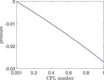
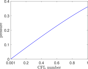
Figure 1: The pressure $\bar{p}_{j}^{n+1}$ obtained by the LF scheme (31) with different parameter $\alpha_{1,n}^{\tt LF}$ and using different CFL numbers. Left: $\alpha_{1,n}^{\tt LF}=\max_{j}{\mathscr{R}}_{1}(\bar{\bf U}_{j}^{n})$; right: $\alpha_{1,n}^{\tt LF}=\max_{j}\alpha_{1}\big{(}\bar{\bf U}_{j+1}^{n},\bar{\bf U}_{j-1}^{n};\sqrt{\bar{\rho}_{j+1}^{n}}/{(\sqrt{\bar{\rho}_{j+1}^{n}}+\sqrt{\bar{\rho}_{j-1}^{n}})}\big{)}$.

In the following, we conduct numerical experiments on several 1D MHD problems with low density, low pressure, strong discontinuity, and/or low plasma-beta $\beta:=2p/|{\bf B}|^{2}$, to demonstrate the accuracy and robustness of the 1D provenly PP high-order methods. Without loss of generality, we take the third-order (${\mathbb{P}}^{2}$-based), discontinuous Galerkin (DG) method, together with the third-order explicit strong stability preserving (SSP) Runge-Kutta time discretization [18], as our base scheme. The LF flux (30) is used with the numerical viscosity parameters satisfying the condition (39). The PP limiter in [11] is employed to enforce the condition (38). According to our analysis in Theorem 3.6, the resulting DG scheme is PP. Unless otherwise stated, all the computations are restricted to the ideal equation of state (3), and the CFL number is taken as 0.15.

5.1.2 Accuracy test

A smooth problem is tested to verify the accuracy of the third-order DG method. It is similar to the one simulated in [51] for testing the PP DG scheme for the Euler equations. The exact solution is given by

$$(\rho,{\bf v},p,{\bf B})({\tt x},t)=(1+0.99\sin({\tt x}-t),~{}1,~{}0,~{}0,~{}1,~{}0.1,~{}0,~{}0),\quad{\tt x}\in[0,2\pi],~{}t\geq 0,$$

which describes a MHD sine wave propagating with low density and $\gamma=1.4$. Table 1 lists the numerical errors at $t=0.1$ in the numerical density and the corresponding convergence rates for the PP third-order DG method at different grid resolutions. The results show that the expected convergence order is achieved.

Table 1: Numerical errors at $t=0.1$ in the density and corresponding convergence rates for the 1D PP third-order DG method at different grid resolutions.

Mesh	$l^{1}$-error	order	$l^{2}$-error	order	$l^{\infty}$-error	order
$40$	2.1268e-4	–	9.5354e-5	–	5.9715e-5	–
$80$	3.7004e-5	2.52	1.6502e-5	2.53	1.0401e-5	2.52
$160$	5.1857e-6	2.84	2.3121e-6	2.84	1.4582e-6	2.83
$320$	6.6087e-7	2.97	2.9467e-7	2.97	1.8587e-7	2.97
$640$	8.2817e-8	3.00	3.6926e-8	3.00	2.3292e-8	3.00
$1280$	1.0358e-8	3.00	4.6185e-9	3.00	2.9133e-9	3.00

5.1.3 Positivity-preserving tests

Two extreme 1D Riemann problems are solved to verify the robustness and PP property of the PP third-order DG scheme.

The first is a 1D vacuum shock tube problem [13] with $\gamma=\frac{5}{3}$ and the initial data given by

$$(\rho,{\bf v},p,{\bf B})({\tt x},0)=\begin{cases}(10^{-12},~{}0,~{}0,~{}0,~{}10^{-12},~{}0,~{}0,~{}0),\quad&x<0,\\ (1,~{}0,~{}0,~{}0,~{}0.5,~{}0,~{}1,~{}0),\quad&x>0.\end{cases}$$

We use this example to demonstrate that the PP DG scheme can handle extremely low density and pressure. The computational domain is taken as $[-0.5,0.5]$. Fig. 2 displays the density and pressure of the numerical solution on the mesh of $200$ cells as well as the highly resolved solution with $2000$ cells at $t=0.1$. In comparison with the results in [13], the low pressure and the low density are both captured correctly and well. The solutions of low resolution and high resolution are in good agreement. The PP third-order DG method works very robustly during the whole simulation. If the PP limiter is not employed to enforce the condition (38), the method breaks down within a few time steps.

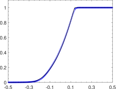
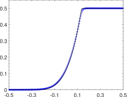
Figure 2: The density (left) and pressure (right) obtained by the PP third-order DG method on the meshes of $200$ cells (symbols “$\circ$”) and $2000$ cells (solid lines), respectively.

The second Riemann problem is extended from the Leblanc problem [51] of gas dynamics by adding a strong magnetic field. The initial condition is

$$(\rho,{\bf v},p,{\bf B})({\tt x},0)=\begin{cases}(2,~{}0,~{}0,~{}0,~{}10^{9},~{}0,~{}5000,~{}5000),\quad&x<0,\\ (0.001,~{}0,~{}0,~{}0,~{}1,~{}0,~{}5000,~{}5000),\quad&x>0.\end{cases}$$

The adiabatic index $\gamma=1.4$, and the computational domain is $[-10,10]$. There exists a very large jump in the initial pressure, and the plasma-beta at the right state is extremely low ($\beta=4\times 10^{-8}$). Successfully simulating this problem is a challenge. As the exact solution contains strong discontinuities, the WENO limiter [33] is implemented right before the PP limiting procedure with the aid of the local characteristic decomposition within the “trouble” cells adaptively detected by the indicator in [23]. To fully resolve the wave structure, a fine mesh is required for such test, see e.g., [51]. Fig. 3 gives the numerical results at $t=0.00003$ obtained by the PP third-order DG method using $3200$ cells and $10000$ cells, respectively. We observe that the strong discontinuities are well captured, and the low resolution and high resolution are in good agreement. In this extreme test, it is also necessary to use the PP limiter to meet the condition (38), otherwise the DG method will break down quickly due to negative numerical pressure.

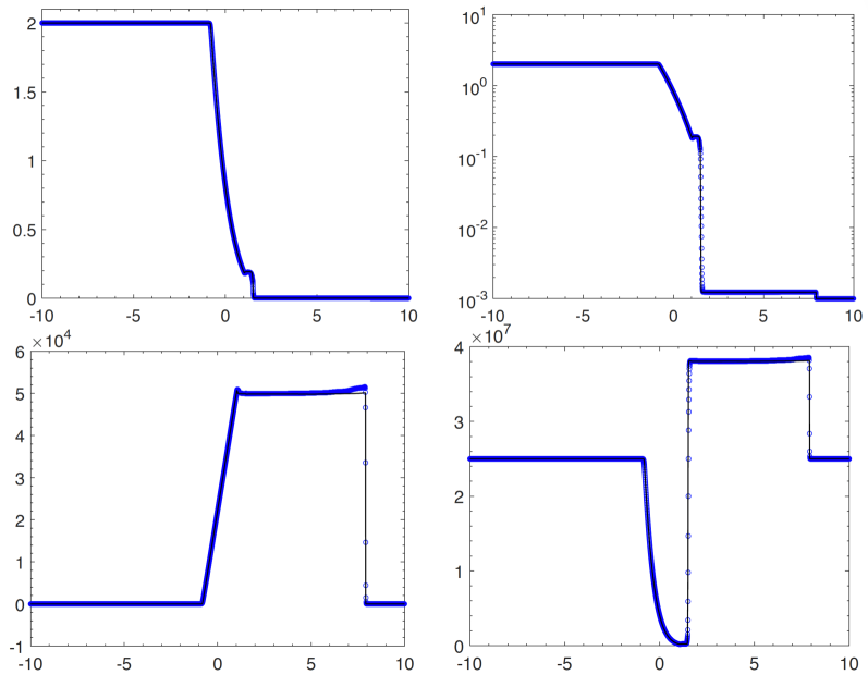
Figure 3: Numerical results at $t=0.00003$ obtained by the PP third-order DG method using $3200$ cells (symbols “$\circ$”) and $10000$ cells (solid lines). Top left: density; top right: log plot of density; bottom left: velocity $v_{1}$; bottom right: magnetic pressure.

5.2 2D case

We now present several 2D numerical examples to further confirm our theoretical analysis and the importance of the proposed discrete divergence-free (DDF) condition.

5.2.1 Simple example

This is a simple test which can be repeated easily by interested readers. We consider the 2D discrete data in (44) with $\gamma=1.4$, $\epsilon=10^{-3}$ and ${\tt p}=10^{-8}$. The states in this data are admissible, and are slight perturbations of the constant state $(1,1,0,0,1,0,0,1+2.5{\tt p})^{\top}$ so that the proposed DDF condition (45) is not satisfied. We then check the pressure $\bar{p}_{ij}^{n+1}$ computed by the 2D LF scheme (42) with $\Delta x=\Delta y$ and different CFL numbers ${\tt C}\in\{0.01,0.02,\cdots,1\}$. The results are shown in Fig. 4, where two sets of parameters $\{\alpha_{\ell,n}^{\tt LF}\}$ are considered. It can be observed that, though the parameters $\{\alpha_{\ell,n}^{\tt LF}\}$ satisfy the condition (47) or are even much larger, the admissibility of all the discrete states at the time level $n$ cannot ensure the positivity of numerical pressure at the next level. This confirms Theorem 4.1 and the importance of DDF condition (45).

Figure 4: The pressure $\bar{p}_{ij}^{n+1}$ obtained by the 2D LF scheme (42) with larger numerical viscosity parameters and using different CFL numbers. Left: $\alpha_{\ell,n}^{\tt LF}=2\max_{ij}{{\mathscr{R}}_{\ell}(\bar{\bf U}^{n}_{ij})}$; right: $\alpha_{\ell,n}^{\tt LF}=50\max_{ij}{{\mathscr{R}}_{\ell}(\bar{\bf U}^{n}_{ij})}$.

In the following, we consider several more practical examples to further verify our theoretical findings for 2D PP high-order schemes, and to seek the numerical evidences for that only enforcing the condition (51) is not sufficient to achieve PP high-order conservative scheme. To this end, we take the locally divergence-free DG methods [24], together with the third-order SSP Runge-Kutta time discretization [18], as the base schemes. We use the PP limiter in [11] to enforce the condition (51). As we have discussed in Section 4.2, the resulting high-order DG schemes do not always preserve the positivity of pressure under all circumstances, because the proposed DDF condition (50) is not always satisfied (although the numerical magnetic field is locally divergence-free within each cell). It is worth mentioning that the locally divergence-free property and the PP limiter can enhance, to a certain extent, the robustness of high-order DG methods.

Without loss of generality, the third-order (${\mathbb{P}}^{2}$-based) DG method is considered. Unless otherwise stated, all the computations are restricted to the ideal equation of state (3) with the adiabatic index $\gamma=\frac{5}{3}$, and the CFL number is taken as 0.15. For the problems involving discontinuity, before using the PP limiter, the WENO limiter [33] with locally divergence-free reconstruction (cf. [54]) is also implemented with the aid of the local characteristic decomposition, to enhance the numerical stability of high-oder DG methods in resolving the strong discontinuities and their interactions. The WENO limiter is only used in the “trouble” cells adaptively detected by the indicator in [23].

5.2.2 Accuracy tests

Two smooth problems are solved to test the accuracy of the ${\mathbb{P}}^{2}$-based DG method with the PP limiter. The first problem, similar to the one simulated in [51], describes a MHD sine wave periodicly propagating within the domain $[0,2\pi]^{2}$ and $\gamma=1.4$. The exact solution is given by

$$(\rho,{\bf v},p,{\bf B})({\tt x},{\tt y},t)=\big{(}1+0.99\sin({\tt x}+{\tt y}-2t),~{}1,~{}1,~{}0,~{}1,~{}0.1,~{}0.1,~{}0\big{)}.$$

The second problem is the vortex problem [13]. The initial condition is a mean flow

$$(\rho,{\bf v},p,{\bf B})({\tt x},{\tt y},0)=(1,~{}1,~{}1,~{}0,~{}1,~{}0,~{}0,~{}0),$$

with vortex perturbations on $v_{1},v_{2},B_{1},B_{2},$ and $p$:

$$(\delta v_{1},\delta v_{2})=\frac{\mu}{\sqrt{2}\pi}{\rm e}^{0.5(1-r^{2})}(-{\tt y},{\tt x}),\quad(\delta B_{1},\delta B_{2})=\frac{\mu}{2\pi}{\rm e}^{0.5(1-r^{2})}(-{\tt y},{\tt x}),$$

$$\delta p=-\frac{\mu^{2}(1+r^{2})}{8\pi^{2}}{\rm e}^{1-r^{2}},$$

where $r=\sqrt{{\tt x}^{2}+{\tt y}^{2}}$, and the vortex strength $\mu=5.389489439$ such that the lowest pressure in the center of the vortex is about $5.3\times 10^{-12}$. The computational domain is $[-10,10]^{2}$ with periodic boundary conditions. Fig. 5 displays the numerical errors obtained by the third-order DG method with the PP limiter at different grid resolutions. The results show that the expected convergence order is achieved, and the PP limiter does not destroy the accuracy.

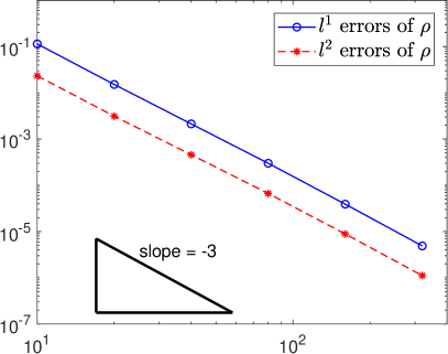
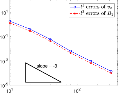
Figure 5: Numerical errors obtained by the third-order DG method at different grid resolutions with $N\times N$ cells. Left: the first 2D smooth problem at $t=0.1$; right: the second 2D smooth problem at $t=0.05$. The horizontal axis denotes the value of $N$.

5.2.3 Benchmark tests

The Orszag-Tang problem (see e.g., [24]) and the rotor problem [6] are benchmark tests widely performed in the literature. Although not extreme, they are simulated by our third-order DG code to verify the high-resolution of the DG method as well as the correctness of our code. The contour plots of the density are shown in Fig. 6 and agree well with those computed in [6, 24]. We observe that the PP limiter does not get turned on, as the condition (51) is automatically satisfied in these simulations.

Figure 6: Numerical solutions of the Orszag-Tang problem with $200\times 200$ cells at $t=2$ (left) and the rotor problem with $400\times 400$ at $t=0.295$ (right) computed by the third-order DG method.

5.2.4 Positivity-preserving tests

Two extreme problems are solved to demonstrate the importance of the proposed conditions (50)–(51) in Theorem 4.11 and validate the estimate in Theorem 4.15.

The first one is the blast problem [6] to verify the importance of enforcing the condition (51) for achieving PP high-order DG methods. This problem describes the propagation of a circular strong fast magneto-sonic shock formulates and propagates into the ambient plasma with low plasma-beta. Initially, the computational domain $[-0.5,0.5]^{2}$ is filled with plasma at rest with unit density and adiabatic index $\gamma=1.4$. The explosion zone $(r<0.1)$ has a pressure of $10^{3}$, while the ambient medium $(r>0.1)$ has a lower pressure of $0.1$, where $r=\sqrt{{\tt x}^{2}+{\tt y}^{2}}$. The magnetic field is initialized in the $\tt x$-direction as $100/\sqrt{4\pi}$. Figure 7 shows the numerical results at $t=0.01$ computed by the third-order DG method with the PP limiter on the mesh of $320\times 320$ uniform cells. We see that the results are highly in agreement with those displayed in [6, 26, 13], and the density profile is well captured with much less oscillations than those shown in [6, 13]. It is noticed that the third-order DG method fails to preserve the positivity of pressure at time $t\approx 2.845\times 10^{-4}$ if the PP limiting procedure is not employed to enforce the condition (51).

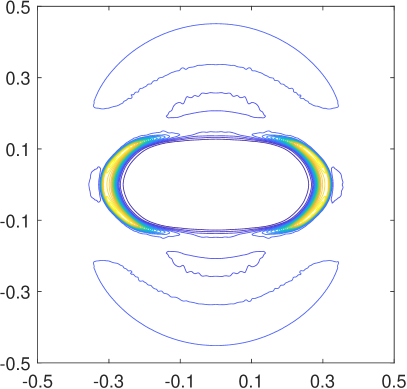
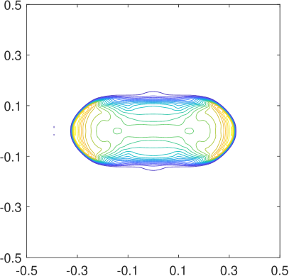
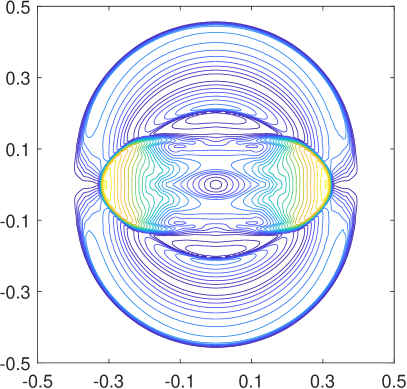
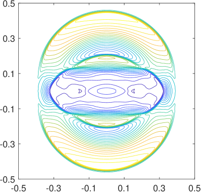
Figure 7: Blast problem: the contour plots of density $\rho$ (top left), pressure $p$ (top right), velocity $|{\bf v}|$ (bottom left) and magnetic pressure $p_{m}$ (bottom right) at $t=0.01$.

To examine the PP property of the third-order DG scheme with the PP limiter, it is necessary to try more challenging test (rather than the standard tests). In a high Mach number jet with strong magnetic field, the internal energy is very small compared to the huge kinetic and magnetic energy, negative pressure may easily appear in the numerical simulation. We consider the Mach 800 dense jet in [4], and add a magnetic field so as to simulate the MHD jet flows. Initially, the computational domain $[-0.5,0.5]\times[0,1.5]$ is filled with a static uniform medium with density of $0.1\gamma$ and unit pressure, where the adiabatic index $\gamma=1.4$. A dense jet is injected in the $\tt y$-direction through the inlet part ($\left|{\tt x}\right|<0.05$) on the bottom boundary (${\tt y}=0$) with density of $\gamma$, unit pressure and speed of $800$. The fixed inflow condition is specified on the nozzle $\{{\tt y}=0,\left|{\tt x}\right|<0.05\}$, and the other boundary conditions are outflow. A magnetic field with a magnitude of $B_{a}$ is initialized along the $\tt y$-direction. The presence of magnetic field makes this test more extreme. A larger $B_{a}$ implies a larger value of $|{\bf v}\cdot{\bf B}|=800B_{a}$, which more easily leads to negative numerical pressure when the DDF condition (50) is violated seriously, as indicated by Theorem 4.15. Therefore, we have a strong motivation to examine the PP property by using this kind of problems.

We first consider a relatively mild setup with a weak magnetic field $B_{a}=\sqrt{20}$. The corresponding plasma-beta ($\beta=0.1$) is not very small. The locally divergence-free DG method with the PP limiter works well for this weak magnetized case, see Fig. 8, which shows the results at $t=0.002$ on the mesh of $400\times 600$ cells. It is seen that the density, gas pressure and velocity profiles are very close to those displayed in [4] for the same jet but without magnetic field. This is not surprising, because the magnetic field is weak in our case. In this simulation, it is also necessary to enforce the condition (51) by the PP limiter, otherwise the DG code will break down at $t\approx 5.58\times 10^{-5}$.

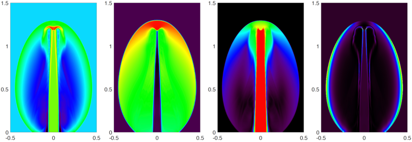
Figure 8: High Mach number jet with a weak magnetic field $B_{a}=\sqrt{20}$. The schlieren images of density logarithm, gas pressure logarithm, velocity $|{\bf v}|$ and magnetic pressure (from left to right) at $t=0.002$.

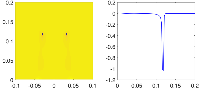
Figure 9: High Mach number jet with a strong magnetic field $B_{a}=\sqrt{200}$. the schlieren image of $\delta_{ij}$ (left) and its slice along ${\tt x}=0.03125$ (right).

To investigate the importance of the proposed DDF condition (50) in Theorem 4.11, we now try to simulate the jet in a moderately magnetized case with $B_{a}=\sqrt{200}$ (the corresponding plasma-beta $\beta=0.01$) on the mesh of $400\times 600$ cells. In this case, the locally divergence-free third-order DG method with the PP limiter breaks down at $t\approx 0.00024$. This failure results from the computed inadmissible cell averages of conservative variables, detected in the four cells centered at points $(-0.03125,0.11625)$, $(-0.03125,0.11875)$, $(0.03125,0.11625)$, and $(0.03125,0.11875)$, respectively. As expected from Theorem 4.15, these inadmissible cell averages correspond to negative numerical pressure (internal energy) due to the violation of DDF condition (50). We recall that Theorem 4.15 implies for the inadmissible cell averages that

$$0\geq{\mathcal{E}}(\bar{\bf U}_{ij}^{n+1})>-\Delta t_{n}\big{(}\bar{\bf v}_{ij}^{n+1}\cdot\bar{\bf B}_{ij}^{n+1}\big{)}{\rm div}_{ij}{\bf B}^{n}.$$

If one defines

$$\begin{split}&{\mathcal{P}}_{ij}:={\mathcal{E}}(\bar{\bf U}_{ij}^{n+1})+\Delta t_{n}\big{(}\bar{\bf v}_{ij}^{n+1}\cdot\bar{\bf B}_{ij}^{n+1}\big{)}{\rm div}_{ij}{\bf B}^{n}>0,\\ &{\mathcal{N}}_{ij}:=-\Delta t_{n}\big{(}\bar{\bf v}_{ij}^{n+1}\cdot\bar{\bf B}_{ij}^{n+1}\big{)}{\rm div}_{ij}{\bf B}^{n},\end{split}$$

and $\delta_{ij}:={\mathcal{N}}_{ij}/{\mathcal{P}}_{ij}$, then $\delta_{ij}\leq-1$ for inadmissible cell averages, and $\delta_{ij}>-1$ for admissible cell averages. As we see from the proof of Theorem 4.15, ${\mathcal{N}}_{ij}$ can be considered as the dominate negative part of ${\mathcal{E}}(\bar{\bf U}_{ij}^{n+1})$ affected by the discrete divergence-error ${\rm div}_{ij}{\bf B}^{n}$, while ${\mathcal{P}}_{ij}$ is the main positive part contributed by the condition (51) enforced by the PP limiter. As evidences of these, Fig. 9 gives the close-up of the schlieren image of $\delta_{ij}$ and its slice along ${\tt x}=0.03125$. It clearly shows the two subregions with small values $\delta_{ij}<-1$, and the four detected cells with inadmissible cell averages are exactly located in those two subregions. This further demonstrates our analysis in Theorem 4.15 and that the DDF condition (50) is really crucial in achieving completely PP schemes in 2D. It is observed that the code fails also on a refined mesh, and also for more strongly magnetized case.

More numerical results further supporting our analysis can be found in [41], where the proposed theoretical techniques are applied to design multi-dimensional provably PP DG schemes via the discretization of symmetrizable ideal MHD equations.

6 Conclusions

We presented the rigorous PP analysis of conservative schemes with the LF flux for one- and multi-dimensional ideal MHD equations. It was based on several important properties of admissible state set, including a novel equivalent form, convexity, orthogonal invariance and the generalized LF splitting properties. The analysis was focused on the finite volume or discontinuous Galerkin schemes on uniform Cartesian meshes. In the 1D case, we proved that the LF scheme with proper numerical viscosity is PP, and the high-order schemes are PP under accessible conditions. In the 2D case, our analysis revealed for the first time that a discrete divergence-free (DDF) condition is crucial for achieving the PP property of schemes for ideal MHD. We proved that the 2D LF scheme with proper numerical viscosity preserves the positivity and the DDF condition. We derived sufficient conditions for achieving 2D PP high-order schemes. Lower bound of the internal energy was derived when the proposed DDF condition was not satisfied, yielding that negative internal energy may be more easily computed in the cases with large $|{\bf v}\cdot{\bf B}|$ and large discrete divergence error. Our analyses were further confirmed by the numerical examples, and extended to the 3D case.

In addition, several usually-expected properties were disproved in this paper. Specifically, we rigorously showed that: (i) the LF splitting property does not always hold; (ii) the 1D LF scheme with standard numerical viscosity or piecewise constant $B_{1}$ is not PP in general, no matter how small the CFL number is; (iii) the 2D LF scheme is not always PP under any CFL condition, unless additional condition like the DDF condition is satisfied. As a result, some existing techniques for PP analysis become inapplicable in the MHD case. These, together with the technical challenges arising from the solenoidal magnetic field and the intrinsic complexity of the MHD system, make the proposed analysis very nontrivial.

From the viewpoint of preserving positivity, our analyses provided a new understanding of the importance of divergence-free condition in robust MHD simulations. Our analyses and novel techniques as well as the provenly PP schemes can also be useful for investigating or designing other PP schemes for ideal MHD. In [41], we applied the proposed analysis approach to develop multi-dimensional probably PP high-order methods for the symmetrizable version of the ideal MHD equations. The extension of the PP analysis to less dissipative numerical fluxes and on more general/unstructured meshes will be studied in a coming paper.

Appendix A Additional Proofs

A.1 Proof of Proposition 2.7

Proof A.1.

We prove it by contradiction. Assume that (8) always holds. Let $\alpha=\chi{\mathscr{R}}_{i}$ with the constant $\chi\geq 1$. For any ${\tt p}\in\big{(}0,\frac{1}{\gamma}\big{)}$, consider the admissible state ${\bf U}=(1,0,0,0,1,0,0,\frac{\tt p}{\gamma-1}+\frac{1}{2})^{\top}$ for an ideal gas. Then (8) implies that

$${\bf U}\pm\frac{{\bf F}_{1}({\bf U})}{\alpha}=\bigg{(}1,\pm\frac{{\tt p}-\frac{1}{2}}{\chi},0,0,1,0,0,\frac{\tt p}{\gamma-1}+\frac{1}{2}\bigg{)}^{\top}\in{\mathcal{G}}.$$

This means, for $\forall{\tt p}\in\big{(}0,\frac{1}{\gamma}\big{)}$,

$$0<{\mathcal{E}}({\bf U}\pm\alpha^{-1}{\bf F}_{1}({\bf U}))=\frac{\tt p}{\gamma-1}-{\frac{1}{2\chi^{2}}}\bigg{(}{\tt p}-\frac{1}{2}\bigg{)}^{2}=:{\mathcal{E}}_{f}({\tt p}),$$

The continuity of ${\mathcal{E}}_{f}({\tt p})$ further implies

$$0\leq\mathop{\lim}\limits_{{\tt p}\to 0^{+}}{\mathcal{E}}_{f}({\tt p})=-\frac{1}{8\chi^{2}}<0,$$

which is a contradiction. Hence (8) does not always hold. The proof is completed.

A.2 Proof of Proposition 2.14

Proof A.2.

The proof is similar to that of Lemma 2.8. Without loss of generality, we only show (21) for $i=1$, while the cases of $i=2$ and $i=3$ can be then proved by using the orthogonal invariance in Lemma 2.6 and similarly to part (ii) of the proof of Lemma 2.8.

For $i=1$, let define

$$\hat{\Pi}_{u}={\bf U}\cdot{\bf n}^{*}+\frac{|{\bf B}^{*}|^{2}}{2},\quad\hat{\Pi}_{f}={\bf F}_{1}({\bf U})\cdot{\bf n}^{*}+v_{i}^{*}\frac{|{\bf B}^{*}|^{2}}{2}-B_{i}({\bf v}^{*}\cdot{\bf B}^{*}).$$

Then it only needs to show

(57) $$\frac{|\hat{\Pi}_{f}|}{\hat{\Pi}_{u}}\leq\widehat{\alpha}_{1}({\bf U},{v}_{1}^{*}),$$

by noting that

(58) $$\hat{\Pi}_{u}=|\hat{\bm{\theta}}|^{2}>0,$$

where the nonzero vector $\hat{\bm{\theta}}\in{\mathbb{R}}^{7}$ is defined as

$$\hat{\bm{\theta}}=\frac{1}{\sqrt{2}}\Big{(}\sqrt{\rho}({\bf v}-{\bf v}^{*}),~{}{\bf B}-{\bf B}^{*},~{}\sqrt{2\rho e}\Big{)}^{\top}.$$

The proof of (57) is divided into the following two steps.

Step 1. Reformulate $\hat{\Pi}_{f}$ into a quadratic form in the variables $\hat{\theta}_{j},1\leq j\leq 7$. Unlike what is required in Lemma 2.8, one cannot require that the coefficients of this quadratic form is independent on ${\bf v}^{*}$ and ${\bf B}^{*}$, but can require those coefficients do not depend on ${v}_{2}^{*}$, $v_{3}^{*}$ and ${\bf B}^{*}$. Similar to the proof of Lemma 2.8, we technically arrange $\hat{\Pi}_{f}$ as

(59) $$\hat{\Pi}_{f}=\frac{1}{2}v_{1}^{*}|{\bf B}-{\bf B}^{*}|^{2}++\frac{\rho v_{1}}{2}|{\bf v}-{\bf v}^{*}|^{2}+v_{1}\rho e+p(v_{1}-v_{1}^{*})+\sum_{j=2}^{3}(B_{j}(v_{1}-v_{1}^{*})-B_{1}(v_{j}-v_{j}^{*}))(B_{j}-B_{j}^{*}).$$

Then we immediately have

(60) $$\hat{\Pi}_{f}=v_{1}^{*}\sum_{j=4}^{6}\hat{\theta}_{j}^{2}+v_{1}\Big{(}\sum_{j=1}^{3}\hat{\theta}_{j}^{2}+\hat{\theta}_{7}^{2}\Big{)}+2{\mathscr{C}}_{s}\hat{\theta}_{1}\hat{\theta}_{7}+\frac{2B_{2}}{\sqrt{\rho}}\hat{\theta}_{1}\hat{\theta}_{5}+\frac{2B_{3}}{\sqrt{\rho}}\hat{\theta}_{1}\hat{\theta}_{6}-\frac{2B_{1}}{\sqrt{\rho}}(\hat{\theta}_{2}\hat{\theta}_{5}+\hat{\theta}_{3}\hat{\theta}_{6}).$$

Step 2. Estimate the upper bound of $\frac{|\hat{\Pi}_{f}|}{\hat{\Pi}_{u}}$. Note that

$$\hat{\Pi}_{f} =v_{1}^{*}\sum_{j=4}^{6}\hat{\theta}_{j}^{2}+v_{1}\Big{(}\sum_{j=1}^{3}\hat{\theta}_{j}^{2}+\hat{\theta}_{7}^{2}\Big{)}+\hat{\bm{\theta}}^{\top}{\bf A}_{7}\hat{\bm{\theta}},$$

where

$${\bf A}_{7}=\begin{pmatrix}0&0&0&0&B_{2}\rho^{-\frac{1}{2}}&B_{3}\rho^{-\frac{1}{2}}&{\mathscr{C}}_{s}\\ 0&0&0&0&-B_{1}\rho^{-\frac{1}{2}}&0&0\\ 0&0&0&0&0&-B_{1}\rho^{-\frac{1}{2}}&0\\ 0&0&0&0&0&0&0\\ B_{2}\rho^{-\frac{1}{2}}&-B_{1}\rho^{-\frac{1}{2}}&0&0&0&0&0\\ B_{3}\rho^{-\frac{1}{2}}&0&-B_{1}\rho^{-\frac{1}{2}}&0&0&0&0\\ {\mathscr{C}}_{s}&0&0&0&0&0&0\end{pmatrix}.$$

The spectral radius of ${\bf A}_{7}$ is ${\mathscr{C}}_{1}$. This gives the following estimate

(61) $$|\hat{\Pi}_{f}| \leq|v_{1}^{*}|\sum_{j=4}^{6}\hat{\theta}_{j}^{2}+|v_{1}|\bigg{(}\sum_{j=1}^{3}\hat{\theta}_{j}^{2}+\hat{\theta}_{7}^{2}\bigg{)}+|\hat{\bm{\theta}}^{\top}{\bf A}_{7}\hat{\bm{\theta}}|$$

$$\leq\max\{|v_{1}|,|v_{1}^{*}|\}|\hat{\bm{\theta}}|^{2}+{\mathscr{C}}_{1}|\hat{\bm{\theta}}|^{2}=\widehat{\alpha}_{1}({\bf U},v_{1}^{*})|\hat{\bm{\theta}}|^{2}=\widehat{\alpha}_{1}({\bf U},v_{1}^{*})\hat{\Pi}_{u}.$$

Therefore, the inequality (57) holds. The proof is completed.

A.3 Deriving generalized LF splitting property by Proposition 2.14

Proposition A.3.

The 1D generalized LF splitting property in Theorem 2.15 holds for any $\alpha$ satisfying

$$\alpha>\widetilde{\alpha}_{1}(\hat{\bf U},\check{\bf U}),$$

where $\widetilde{\alpha}_{1}$ is a different lower bound given by

$$\widetilde{\alpha}_{1}(\hat{\bf U},\check{\bf U}):=\max\{\hat{\mathscr{C}}_{1},\check{\mathscr{C}}_{1}\}+\max\{|\hat{v}_{1}|+\hat{\mathscr{D}}_{1},|\check{v}_{1}|+\check{\mathscr{D}}_{1}\}$$

with

$$\hat{\mathscr{D}}_{1}:=\frac{|\hat{p}_{tot}-\hat{B}_{1}^{2}|}{\hat{\rho}(A_{1}-\hat{v}_{1})},\qquad\check{\mathscr{D}}_{1}:=\frac{|\check{p}_{tot}-\check{B}_{1}^{2}|}{\check{\rho}(A_{1}+\check{v}_{1})},\qquad A_{1}:=\max\{|\hat{v}_{1}|,|\check{v}_{1}|\}+\max\{\hat{\mathscr{C}}_{1},\check{\mathscr{C}}_{1}\}.$$

For the ideal EOS (3), the property also holds for any $\alpha>\widetilde{\widetilde{\alpha}}_{1}(\hat{\bf U},\check{\bf U})$, where

$$\alpha>\widetilde{\widetilde{\alpha}}_{1}(\hat{\bf U},\check{\bf U}):=\max\{\hat{\mathcal{C}}_{1},\check{\mathcal{C}}_{1}\}+\max\{|\hat{v}_{1}|+\hat{\mathcal{D}}_{1},|\check{v}_{1}|+\check{\mathcal{D}}_{1}\}$$

with

$$\hat{\mathcal{D}}_{1}:=\frac{|\hat{p}_{tot}-\hat{B}_{1}^{2}|}{\hat{\rho}({\mathcal{A}}_{1}-\hat{v}_{1})},\qquad\check{\mathcal{D}}_{1}:=\frac{|\check{p}_{tot}-\check{B}_{1}^{2}|}{\check{\rho}({\mathcal{A}}_{1}+\check{v}_{1})},\qquad{\mathcal{A}}_{1}:=\max\{|\hat{v}_{1}|,|\check{v}_{1}|\}+\max\{\hat{\mathcal{C}}_{1},\check{\mathcal{C}}_{1}\}.$$

Proof A.4.

Let $\overline{\rho}$, $\overline{\bf v}$ and $\overline{\bf B}$ respectively denote the density, velocity and magnetic field corresponding to $\overline{\bf U}$. Note that

$$\widetilde{\alpha}_{1}(\hat{\bf U},\check{\bf U})>\max\{|\hat{v}_{1}|,|\check{v}_{1}|\},$$

which implies

$$\overline{\rho}=\frac{1}{2}\bigg{(}\hat{\rho}\Big{(}1-\frac{\hat{v}_{1}}{\alpha}\Big{)}+\check{\rho}\Big{(}1+\frac{\check{v}_{1}}{\alpha}\Big{)}\bigg{)}>0,$$

for any $\alpha>\widetilde{\alpha}_{1}(\hat{\bf U},\check{\bf U})$. Then it only needs to show ${\mathcal{E}}(\overline{\bf U})>0$. Define $\overline{\bf n}=\big{(}\frac{|\overline{\bf v}|^{2}}{2},~{}-\overline{\bf v},~{}-\overline{\bf B},~{}1\big{)}^{\top},$ then we can reformulate $2{\mathcal{E}}(\overline{\bf U})$ as

$$2{\mathcal{E}}(\overline{\bf U}) =2\overline{\bf U}\cdot\overline{\bf n}+{|\overline{\bf B}|^{2}}=\bigg{(}\hat{\bf U}-\frac{{\bf F}_{1}(\hat{\bf U})}{\alpha}+\check{\bf U}+\frac{{\bf F}_{1}(\check{\bf U})}{\alpha}\bigg{)}\cdot\overline{\bf n}+{|\overline{\bf B}|^{2}}$$

$$=\bigg{[}\bigg{(}\hat{\bf U}-\frac{{\bf F}_{1}(\hat{\bf U})}{\alpha}\bigg{)}\cdot\overline{\bf n}+\frac{|\overline{\bf B}|^{2}}{2}-\frac{1}{\alpha}\bigg{(}\overline{v}_{1}\frac{|\overline{\bf B}|^{2}}{2}-\hat{B}_{1}(\overline{\bf v}\cdot\overline{\bf B})\bigg{)}\bigg{]}$$

$$\quad+\bigg{[}\bigg{(}\check{\bf U}+\frac{{\bf F}_{1}(\check{\bf U})}{\alpha}\bigg{)}\cdot\overline{\bf n}+\frac{|\overline{\bf B}|^{2}}{2}+\frac{1}{\alpha}\bigg{(}\overline{v}_{1}\frac{|\overline{\bf B}|^{2}}{2}-\check{B}_{1}(\overline{\bf v}\cdot\overline{\bf B})\bigg{)}\bigg{]}$$

(62) $$=:\Pi_{1}+\Pi_{2},$$

where the DDF condition (22) has been used. We then use Proposition 2.14 to prove $\Pi_{i}>0,i=1,2,$ by verifying that

$$\widetilde{\alpha}_{1}(\hat{\bf U},\check{\bf U})\geq\widehat{\alpha}_{1}(\hat{\bf U},\overline{v}_{1}),\qquad\widetilde{\alpha}_{1}(\hat{\bf U},\check{\bf U})\geq\widehat{\alpha}_{1}(\check{\bf U},\overline{v}_{1}).$$

It is sufficient to show that

$$\widetilde{\alpha}_{1}(\hat{\bf U},\check{\bf U})\geq\max\{|\hat{v}_{1}|,|\overline{v}_{1}|,|\check{v}_{1}|\}+\max\{\hat{\mathscr{C}}_{1},\check{\mathscr{C}}_{1}\},$$

or equivalently

$$\max\{|\hat{v}_{1}|+\hat{\mathscr{D}}_{1},|\check{v}_{1}|+\check{\mathscr{D}}_{1}\}\geq\max\{|\hat{v}_{1}|,|\overline{v}_{1}|,|\check{v}_{1}|\},$$

which can be verified easily by noting that

$$A_{1}\leq\widetilde{\alpha}_{1}(\hat{\bf U},\check{\bf U})<\alpha.$$

Therefore, $\Pi_{i}>0,i=1,2,$ by Proposition 2.14. It follows from (62) that ${\mathcal{E}}(\overline{\bf U})>0$. Hence $\overline{\bf U}\in{\mathcal{G}}$ for any $\alpha>{\widetilde{\alpha}}_{1}(\hat{\bf U},\check{\bf U})$.

In the ideal EOS case, by noting that ${\mathcal{C}}_{1}>{\mathscr{C}}_{1}$, similar arguments imply $\overline{\bf U}\in{\mathcal{G}}$ for any $\alpha>\widetilde{\widetilde{\alpha}}_{1}(\hat{\bf U},\check{\bf U})$. The proof is completed.

Remark A.5.

It is worth mentioning that the estimated lower bounds $\widetilde{\alpha}_{1}$ and $\widetilde{\widetilde{\alpha}}_{1}$ are not as sharp as the bound $\alpha_{1}$ in Theorem 2.15. Note that here the lower bound of $\alpha$ is said to be sharper if it is smaller, indicating that the resulting generalized LF splitting properties hold for a larger range of $\alpha$. The sharper (i.e., smaller) lower bound is more desirable, because it corresponds to a less dissipative LF flux (allowing smaller numerical viscosity) in our provably PP schemes.

Remark A.6.

Let define

$${\mathscr{H}}_{i}({\bf U}):=|v_{i}|+\frac{|p_{tot}-B_{i}^{2}|}{\rho{\mathscr{C}}_{i}},\quad{\mathcal{H}}_{i}({\bf U}):=|v_{i}|+\frac{|p_{tot}-\ B_{i}^{2}|}{\rho{\mathcal{C}}_{i}}.$$

Since $\widetilde{\alpha}_{1}$ and $\widetilde{\widetilde{\alpha}}_{1}$ in Proposition A.3 only play the role of lower range bounds, they can be replaced with some simpler but larger (not sharp) ones, e.g.,

$$\widetilde{\alpha}_{1}(\hat{\bf U},\check{\bf U})\qquad\longleftrightarrow\qquad\max\{\hat{\mathscr{C}}_{1},\check{\mathscr{C}}_{1}\}+\max\big{\{}{\mathscr{H}}_{1}(\hat{\bf U}),{\mathscr{H}}_{1}(\check{\bf U})\big{\}},$$

$$\widetilde{\widetilde{\alpha}}_{1}(\hat{\bf U},\check{\bf U})\qquad\longleftrightarrow\qquad\max\{\hat{\mathcal{C}}_{1},\check{\mathcal{C}}_{1}\}+\max\big{\{}{\mathcal{H}}_{1}(\hat{\bf U}),{\mathcal{H}}_{1}(\check{\bf U})\big{\}}.$$

The 2D and 3D generalized LF splitting properties can also be similarly derived by Proposition 2.14.

Appendix B 3D Positivity-Preserving Analysis

The extension of our PP analysis to 3D case is straightforward, and for completeness, also given as follows. We only present the main theorems, and omit the proofs, which are very similar to the 2D case except for using the 3D generalized LF splitting property in Theorem 2.22.

To avoid confusing subscripts, the symbols $({\tt x},{\tt y},{\tt z})$ are used to denote the variables $(x_{1},x_{2},x_{3})$ in (1). Assume that the 3D spatial domain is divided into a uniform cuboid mesh with cells $\big{\{}I_{ijk}=({\tt x}_{i-\frac{1}{2}},{\tt x}_{i+\frac{1}{2}})\times({\tt y}_{j-\frac{1}{2}},{\tt y}_{j+\frac{1}{2}})\times({\tt z}_{k-\frac{1}{2}},{\tt z}_{k+\frac{1}{2}})\big{\}}$. The spatial step-sizes in ${\tt x},{\tt y},{\tt z}$ directions are denoted by $\Delta x,\Delta y,\Delta z$ respectively. The time interval is also divided into the mesh $\{t_{0}=0,t_{n+1}=t_{n}+\Delta t_{n},n\geq 0\}$ with the time step size $\Delta t_{n}$ determined by the CFL condition. We use $\bar{\bf U}_{ijk}^{n}$ to denote the numerical approximation to the cell average of the exact solution over $I_{ijk}$ at time $t_{n}$.

B.1 First-order scheme

We consider the 3D first-order LF scheme

(63) $$\begin{split}\bar{\bf U}_{ijk}^{n+1}=\bar{\bf U}_{ijk}^{n}&-\frac{\Delta t_{n}}{\Delta x}\Big{(}\hat{\bf F}_{1}(\bar{\bf U}_{ijk}^{n},\bar{\bf U}_{i+1,j,k}^{n})-\hat{\bf F}_{1}(\bar{\bf U}_{i-1,j,k}^{n},\bar{\bf U}_{ijk}^{n})\Big{)}\\ &-\frac{\Delta t_{n}}{\Delta y}\Big{(}\hat{\bf F}_{2}(\bar{\bf U}_{ijk}^{n},\bar{\bf U}_{i,j+1,k}^{n})-\hat{\bf F}_{2}(\bar{\bf U}_{i,j-1,k}^{n},\bar{\bf U}_{ijk}^{n})\Big{)}\\ &-\frac{\Delta t_{n}}{\Delta z}\Big{(}\hat{\bf F}_{3}(\bar{\bf U}_{ijk}^{n},\bar{\bf U}_{i,j,k+1}^{n})-\hat{\bf F}_{3}(\bar{\bf U}_{i,j,k-1}^{n},\bar{\bf U}_{ijk}^{n})\Big{)},\end{split}$$

where $\hat{\bf F}_{\ell}(\cdot,\cdot),\ell=1,2,3,$ are the LF fluxes in (30). We have the following conclusions.

Theorem B.1.

Let $\alpha_{\ell,n}^{\tt LF}=\chi\max_{ijk}{{\mathscr{R}}_{\ell}(\bar{\bf U}^{n}_{ij})}$ with the constant $\chi\geq 1$, and

$$\Delta t_{n}=\frac{{\tt C}}{\alpha_{1,n}^{\tt LF}/\Delta x+\alpha_{2,n}^{\tt LF}/\Delta y+\alpha_{3,n}^{\tt LF}/\Delta z},$$

where ${\tt C}>0$ is the CFL number. For any given constants $\chi$ and $\tt C$, there always exists a set of admissible states $\{\bar{\bf U}_{ijk}^{n},\forall i,j,k\}$ such that the solution $\bar{\bf U}_{ijk}^{n+1}$ of (63) does not belong to $\mathcal{G}$. In other words, for any given $\chi$ and $\tt C$, the admissibility of $\{\bar{\bf U}_{ijk}^{n},\forall i,j,k\}$ does not always guarantee that $\bar{\bf U}_{ijk}^{n+1}\in{\mathcal{G}}$, $\forall i,j,k$.

Theorem B.2.

If for all $i,j,k$, $\bar{\bf U}_{ijk}^{n}\in{\mathcal{G}}$ and satisfies the following DDF condition

(64) $$\begin{split}&\mbox{\rm div}_{ijk}\bar{\bf B}^{n}:=\frac{\left(\bar{B}_{1}\right)_{i+1,j,k}^{n}-\left(\bar{B}_{1}\right)_{i-1,j,k}^{n}}{2\Delta x}\\ &+\frac{\left(\bar{B}_{2}\right)_{i,j+1,k}^{n}-\left(\bar{B}_{2}\right)_{i,j-1,k}^{n}}{2\Delta y}+\frac{\left(\bar{B}_{3}\right)_{i,j,k+1}^{n}-\left(\bar{B}_{3}\right)_{i,j,k-1}^{n}}{2\Delta z}=0,\end{split}$$

then the solution $\bar{\bf U}_{ijk}^{n+1}$ of (63) always belongs to ${\mathcal{G}}$ under the CFL condition

(65) $$0<\frac{\alpha_{1,n}^{\tt LF}\Delta t_{n}}{\Delta x}+\frac{\alpha_{2,n}^{\tt LF}\Delta t_{n}}{\Delta y}+\frac{\alpha_{3,n}^{\tt LF}\Delta t_{n}}{\Delta z}\leq 1,$$

where the parameters $\{\alpha_{\ell,n}^{\tt LF}\}$ satisfy

(66) $$\begin{gathered}\alpha_{1,n}^{\tt LF}>\max_{i,j,k}\alpha_{1}(\bar{\bf U}_{i+1,j,k}^{n},\bar{\bf U}_{i-1,j,k}^{n}),\quad\alpha_{2,n}^{\tt LF}>\max_{i,j,k}\alpha_{2}(\bar{\bf U}_{i,j+1,k}^{n},\bar{\bf U}_{i,j-1,k}^{n}),\\ \alpha_{3,n}^{\tt LF}>\max_{i,j,k}\alpha_{3}(\bar{\bf U}_{i,j,k+1}^{n},\bar{\bf U}_{i,j,k-1}^{n}).\end{gathered}$$

Theorem B.3.

For the LF scheme (63), the divergence error

$$\varepsilon_{\infty}^{n}:=\max_{ijk}\left|{\rm div}_{ijk}\bar{\bf B}^{n}\right|,$$

does not grow with $n$ under the condition (65). Furthermore, the numerical solutions $\{\bar{\bf U}_{ijk}^{n}\}$ satisfy (64) for all $i,j,k$ and $n\in\mathbb{N}$, if (64) holds for the discrete initial data $\{\bar{\bf U}_{ijk}^{0}\}$.

Theorem B.4.

Assume that the discrete initial data $\{\bar{\bf U}_{ijk}^{0}\}$ are admissible and satisfy (64), which can be met by, e.g., the following second-order approximation

$$\Big{(}\bar{\rho}_{ijk}^{0},\bar{\bf m}_{ijk}^{0},\overline{(\rho e)}_{ijk}^{0}\Big{)}=\frac{1}{\Delta x\Delta y\Delta z}\iint_{I_{ijk}}\big{(}\rho,{\bf m},\rho e\big{)}({\tt x},{\tt y},{\tt z},0)d{\tt x}d{\tt y}d{\tt z},$$

$$\left(\bar{B}_{1}\right)_{ijk}^{0}=\frac{1}{4\Delta y\Delta z}\int_{{\tt y}_{j-1}}^{{\tt y}_{j+1}}\int_{{\tt z}_{k-1}}^{{\tt z}_{k+1}}B_{1}({\tt x}_{i},{\tt y},{\tt z},0)d{\tt y}d{\tt z},$$

$$\left(\bar{B}_{2}\right)_{ijk}^{0}=\frac{1}{4\Delta x\Delta z}\int_{{\tt x}_{i-1}}^{{\tt x}_{i+1}}\int_{{\tt z}_{k-1}}^{{\tt z}_{k+1}}B_{2}({\tt x},{\tt y}_{j},{\tt z},0)d{\tt x}d{\tt z},$$

$$\left(\bar{B}_{3}\right)_{ijk}^{0}=\frac{1}{4\Delta x\Delta y}\int_{{\tt x}_{i-1}}^{{\tt x}_{i+1}}\int_{{\tt y}_{j-1}}^{{\tt y}_{j+1}}B_{3}({\tt x},{\tt y},{\tt z}_{k},0)d{\tt x}d{\tt y},$$

$$~{}\bar{E}_{ijk}^{0}=\overline{(\rho e)}_{ijk}^{0}+\frac{1}{2}\left(\frac{|\bar{\bf m}_{ijk}^{0}|^{2}}{\bar{\rho}_{ijk}^{0}}+|\bar{\bf B}_{ijk}^{0}|^{2}\right).$$

If the parameters $\{\alpha_{\ell,n}^{\tt LF}\}$ satisfy (66), then under the CFL condition (65), the LF scheme (63) preserve both $\bar{\bf U}_{ijk}^{n+1}\in{\mathcal{G}}$ and the DDF condition (64) for all $i$, $j$, $k$, and $n\in\mathbb{N}$.

B.2 High-order schemes

We focus on the forward Euler method for time discretization, and our analysis also works for high-order explicit time discretization using the SSP methods [18]. To achieve high-order accuracy, the approximate solution polynomials ${\bf U}_{ijk}^{n}({\tt x},{\tt y},{\tt z})$ of degree $\tt K$ are also built, as approximation to the exact solution ${\bf U}({\tt x},{\tt y},{\tt z},t_{n})$ within $I_{ijk}$. Such polynomial vector ${\bf U}_{ijk}^{n}({\tt x},{\tt y},{\tt z})$ is, either reconstructed in the finite volume methods from the cell averages $\{\bar{\bf U}_{ijk}^{n}\}$ or evolved in the DG methods. Moreover, the cell average of ${\bf U}_{ijk}^{n}({\tt x},{\tt y},{\tt z})$ over $I_{ijk}$ is $\bar{\bf U}_{ijk}^{n}$.

Let $\{{\tt x}_{i}^{(\mu)}\}_{\mu=1}^{\tt Q}$, $\{{\tt y}_{j}^{(\mu)}\}_{\mu=1}^{\tt Q}$ and $\{{\tt z}_{j}^{(\mu)}\}_{\mu=1}^{\tt Q}$ denote the $\tt Q$-point Gauss quadrature nodes in the intervals $[{\tt x}_{i-\frac{1}{2}},{\tt x}_{i+\frac{1}{2}}]$, $[{\tt y}_{j-\frac{1}{2}},{\tt y}_{j+\frac{1}{2}}]$ and $[{\tt z}_{k-\frac{1}{2}},{\tt z}_{k+\frac{1}{2}}]$, respectively. Let $\{\omega_{\mu}\}_{\mu=1}^{\tt Q}$ be the associated weights satisfying $\sum_{\mu=1}^{\tt Q}\omega_{\mu}=1$. With the 2D tensorized quadrature rule for approximating the integrals of numerical fluxes on cell interfaces, a finite volume scheme or discrete equation for the cell average in the DG method can be written as

(67) $$\begin{split}\bar{\bf U}_{ijk}^{n+1}&=\bar{\bf U}_{ijk}^{n}-\frac{\Delta t_{n}}{\Delta x}\sum\limits_{\mu,\nu}\omega_{\mu}\omega_{\nu}\left(\hat{\bf F}_{1}({\bf U}^{-,\mu,\nu}_{i+\frac{1}{2},j,k},{\bf U}^{+,\mu,\nu}_{i+\frac{1}{2},j,k})-\hat{\bf F}_{1}({\bf U}^{-,\mu,\nu}_{i-\frac{1}{2},j,k},{\bf U}^{+,\mu,\nu}_{i-\frac{1}{2},j,k})\right)\\ &\quad-\frac{\Delta t_{n}}{\Delta y}\sum\limits_{\mu,\nu}\omega_{\mu}\omega_{\nu}\left(\hat{\bf F}_{2}({\bf U}^{\mu,-,\nu}_{i,j+\frac{1}{2},k},{\bf U}^{\mu,+,\nu}_{i,j+\frac{1}{2},k})-\hat{\bf F}_{2}({\bf U}^{\mu,-,\nu}_{i,j-\frac{1}{2},k},{\bf U}^{\mu,+,\nu}_{i,j-\frac{1}{2},k})\right)\\ &\quad-\frac{\Delta t_{n}}{\Delta z}\sum\limits_{\mu,\nu}\omega_{\mu}\omega_{\nu}\left(\hat{\bf F}_{3}({\bf U}^{\mu,\nu,-}_{i,j,k+\frac{1}{2}},{\bf U}^{\mu,\nu,+}_{i,j,k+\frac{1}{2}})-\hat{\bf F}_{3}({\bf U}^{\mu,\nu,-}_{i,j,k-\frac{1}{2}},{\bf U}^{\mu,\nu,+}_{i,j,k-\frac{1}{2}})\right),\end{split}$$

where $\hat{\bf F}_{\ell},\ell=1,2,3$ are the LF fluxes in (30), and the limiting values are given by

$${\bf U}^{-,\mu,\nu}_{i+\frac{1}{2},j,k}={\bf U}_{ijk}^{n}({\tt x}_{i+\frac{1}{2}},{\tt y}_{j}^{(\mu)},{\tt z}_{k}^{(\nu)}),\qquad{\bf U}^{+,\mu,\nu}_{i-\frac{1}{2},j,k}={\bf U}_{ijk}^{n}({\tt x}_{i-\frac{1}{2}},{\tt y}_{j}^{(\mu)},{\tt z}_{k}^{(\nu)}),$$

$${\bf U}^{\mu,-,\nu}_{i,j+\frac{1}{2},k}={\bf U}_{ijk}^{n}({\tt x}_{i}^{(\mu)},{\tt y}_{j+\frac{1}{2}},{\tt z}_{k}^{(\nu)}),\qquad{\bf U}^{\mu,+,\nu}_{i,j-\frac{1}{2},k}={\bf U}_{ijk}^{n}({\tt x}_{i}^{(\mu)},{\tt y}_{j-\frac{1}{2}},{\tt z}_{k}^{(\nu)}),$$

$${\bf U}^{\mu,\nu,-}_{i,j,k+\frac{1}{2}}={\bf U}_{ijk}^{n}({\tt x}_{i}^{(\mu)},{\tt y}_{j}^{(\nu)},{\tt z}_{k+\frac{1}{2}}),\qquad{\bf U}^{\mu,\nu,+}_{i,j,k-\frac{1}{2}}={\bf U}_{ijk}^{n}({\tt x}_{i}^{(\mu)},{\tt y}_{j}^{(\nu)},{\tt z}_{k-\frac{1}{2}}).$$

For the accuracy requirement, $\tt Q$ should satisfy: ${\tt Q}\geq{\tt K}+1$ for a $\mathbb{P}^{\tt K}$-based DG method, or ${\tt Q}\geq({\tt K}+1)/2$ for a $({\tt K}+1)$-th order finite volume scheme.

We denote

$$\overline{(B_{1})}_{i+\frac{1}{2},j,k}^{\mu,\nu}:=\frac{1}{2}\left((B_{1})_{i+\frac{1}{2},j,k}^{-,\mu,\nu}+(B_{1})_{i+\frac{1}{2},j,k}^{+,\mu,\nu}\right),$$

$$\overline{(B_{2})}_{i,j+\frac{1}{2},k}^{\mu,\nu}:=\frac{1}{2}\left((B_{2})_{i,j+\frac{1}{2},k}^{\mu,-,\nu}+(B_{2})_{i,j+\frac{1}{2},k}^{\mu,+,\nu}\right),$$

$$\overline{(B_{3})}_{i,j,k+\frac{1}{2}}^{\mu,\nu}:=\frac{1}{2}\left((B_{3})_{i,j,k+\frac{1}{2}}^{\mu,\nu,-}+(B_{3})_{i,j,k+\frac{1}{2}}^{\mu,\nu,+}\right),$$

and define the discrete divergences of the numerical magnetic field ${\bf B}^{n}({\tt x},{\tt y},{\tt z})$ as

$${\rm div}_{ijk}{\bf B}^{n}:=\frac{\sum\limits_{\mu,\nu}\omega_{\mu}\omega_{\nu}\left(\overline{(B_{1})}_{i+\frac{1}{2},j,k}^{\mu,\nu}-\overline{(B_{1})}_{i-\frac{1}{2},j,k}^{\mu,\nu}\right)}{\Delta x}$$

$$+\frac{\sum\limits_{\mu,\nu}\omega_{\mu}\omega_{\nu}\left(\overline{(B_{2})}_{i,j+\frac{1}{2},k}^{\mu,\nu}-\overline{(B_{2})}_{i,j-\frac{1}{2},k}^{\mu,\nu}\right)}{\Delta y}+\frac{\sum\limits_{\mu,\nu}\omega_{\mu}\omega_{\nu}\left(\overline{(B_{3})}_{i,j,k+\frac{1}{2}}^{\mu,\nu}-\overline{(B_{3})}_{i,j,k-\frac{1}{2}}^{\mu,\nu}\right)}{\Delta z}.$$

Let $\{\hat{\tt x}_{i}^{(\delta)}\}_{\delta=1}^{\tt L}$, $\{\hat{\tt y}_{j}^{(\nu)}\}_{\delta=1}^{\tt L}$ and $\{\hat{\tt z}_{k}^{(\delta)}\}_{\delta=1}^{\tt L}$ be the $\tt L$-point Gauss-Lobatto quadrature nodes in the intervals $[{\tt x}_{i-\frac{1}{2}},{\tt x}_{i+\frac{1}{2}}]$, $[{\tt y}_{j-\frac{1}{2}},{\tt y}_{j+\frac{1}{2}}]$ and $[{\tt z}_{k-\frac{1}{2}},{\tt z}_{k+\frac{1}{2}}]$, respectively, and $\{\hat{\omega}_{\delta}\}_{\delta=1}^{\tt L}$ be associated weights satisfying $\sum_{\delta=1}^{\tt L}\hat{\omega}_{\delta}=1$, where ${\tt L}\geq\frac{{\tt K}+3}{2}$ such that the associated quadrature has algebraic precision of at least degree ${\tt K}$. Then we have the following sufficient conditions for that the high-order scheme (67) is PP.

Theorem B.5.

If the polynomial vectors $\{{\bf U}_{ijk}^{n}({\tt x},{\tt y},{\tt z})\}$ satisfy:

(68) $$\mbox{\rm div}_{ijk}{\bf B}^{n}=0,\quad\forall i,j,k,$$

(69) $${\bf U}_{ijk}^{n}({\bf x})\in{\mathcal{G}},\quad\forall{\bf x}\in{\Theta}_{ijk},\forall i,j,k,$$

with ${\Theta}_{ijk}:=\big{\{}(\hat{\tt x}_{i}^{(\delta)},{\tt y}_{j}^{(\mu)},{\tt z}_{k}^{(\nu)}),~{}({\tt x}_{i}^{(\mu)},\hat{\tt y}_{j}^{(\delta)},{\tt z}_{k}^{(\nu)}),~{}({\tt x}_{i}^{(\mu)},{\tt y}_{j}^{(\nu)},\hat{\tt z}_{k}^{(\delta)}),\forall\mu,\nu,\delta\big{\}},$ then the scheme (67) always preserves $\bar{\bf U}_{ijk}^{n+1}\in{\mathcal{G}}$ under the CFL condition

(70) $$0<\frac{\alpha_{1,n}^{\tt LF}\Delta t_{n}}{\Delta x}+\frac{\alpha_{2,n}^{\tt LF}\Delta t_{n}}{\Delta y}+\frac{\alpha_{3,n}^{\tt LF}\Delta t_{n}}{\Delta z}\leq\hat{\omega}_{1},$$

where the parameters $\{\alpha_{\ell,n}^{\tt LF}\}$ satisfy

(71) $$\begin{split}&\alpha_{1,n}^{\tt LF}>\max_{i,j,k,\mu,\nu}\alpha_{1}\big{(}{\bf U}_{i+\frac{1}{2},j,k}^{\pm,\mu,\nu},{\bf U}_{i-\frac{1}{2},j,k}^{\pm,\mu,\nu}\big{)},\\ &\alpha_{2,n}^{\tt LF}>\max_{i,j,k,\mu,\nu}\alpha_{2}\big{(}{\bf U}_{i,j+\frac{1}{2},k}^{\mu,\pm,\nu},{\bf U}_{i,j-\frac{1}{2},k}^{\mu,\pm,\nu}\big{)},\\ &\alpha_{3,n}^{\tt LF}>\max_{i,j,k,\mu,\nu}\alpha_{3}\big{(}{\bf U}_{i,j,k+\frac{1}{2}}^{\mu,\nu,\pm},{\bf U}_{i,j,k-\frac{1}{2}}^{\mu,\nu,\pm}\big{)}.\end{split}$$

Lower bound of the internal energy can also be estimated when the DDF condition (68) is not satisfied.

Theorem B.6.

Assume the polynomial vectors $\{{\bf U}_{ijk}^{n}({\tt x},{\tt y},{\tt z})\}$ satisfy (69), and the parameters $\{\alpha_{\ell,n}^{\tt LF}\}$ satisfy (71). Then under the CFL condition (70), the solution $\bar{\bf U}_{ijk}^{n+1}$ of the scheme (67) satisfies that $\bar{\rho}_{ijk}^{n+1}>0$, and

$${\mathcal{E}}(\bar{\bf U}_{ijk}^{n+1})>-\Delta t_{n}\big{(}\bar{\bf v}_{ijk}^{n+1}\cdot\bar{\bf B}_{ijk}^{n+1}\big{)}{\rm div}_{ijk}{\bf B}^{n},$$

where $\bar{\bf v}_{ijk}^{n+1}:=\bar{\bf m}_{ijk}^{n+1}/\bar{\rho}^{n+1}_{ijk}$.

References

- [1] R. Artebrant and M. Torrilhon, Increasing the accuracy in locally divergence-preserving finite volume schemes for MHD, J. Comput. Phys., 227 (2008), pp. 3405–3427.
- [2] D. S. Balsara, Second-order-accurate schemes for magnetohydrodynamics with divergence-free reconstruction, Astrophys. J. Suppl. Ser., 151 (2004), pp. 149–184.
- [3] D. S. Balsara, Divergence-free reconstruction of magnetic fields and WENO schemes for magnetohydrodynamics, J. Comput. Phys., 228 (2009), pp. 5040–5056.
- [4] D. S. Balsara, Self-adjusting, positivity preserving high order schemes for hydrodynamics and magnetohydrodynamics, J. Comput. Phys., 231 (2012), pp. 7504–7517.
- [5] D. S. Balsara and D. Spicer, Maintaining pressure positivity in magnetohydrodynamic simulations, J. Comput. Phys., 148 (1999), pp. 133–148.
- [6] D. S. Balsara and D. Spicer, A staggered mesh algorithm using high order Godunov fluxes to ensure solenoidal magnetic fields in magnetohydrodynamic simulations, J. Comput. Phys., 149 (1999), pp. 270–292.
- [7] F. Bouchut, C. Klingenberg, and K. Waagan, A multiwave approximate Riemann solver for ideal MHD based on relaxation. I: theoretical framework, Numer. Math., 108 (2007), pp. 7–42.
- [8] F. Bouchut, C. Klingenberg, and K. Waagan, A multiwave approximate Riemann solver for ideal MHD based on relaxation II: numerical implementation with 3 and 5 waves, Numer. Math., 115 (2010), pp. 647–679.
- [9] J. U. Brackbill and D. C. Barnes, The effect of nonzero on the numerical solution of the magnetodyndrodynamic equations, J. Comput. Phys., 35 (1980), pp. 426–430.
- [10] P. Chandrashekar and C. Klingenberg, Entropy stable finite volume scheme for ideal compressible MHD on 2-D Cartesian meshes, SIAM J. Numer. Anal., 54 (2016), pp. 1313–1340.
- [11] Y. Cheng, F. Li, J. Qiu, and L. Xu, Positivity-preserving DG and central DG methods for ideal MHD equations, J. Comput. Phys., 238 (2013), pp. 255–280.
- [12] A. J. Christlieb, X. Feng, D. C. Seal, and Q. Tang, A high-order positivity-preserving single-stage single-step method for the ideal magnetohydrodynamic equations, J. Comput. Phys., 316 (2016), pp. 218–242.
- [13] A. J. Christlieb, Y. Liu, Q. Tang, and Z. Xu, Positivity-preserving finite difference weighted ENO schemes with constrained transport for ideal magnetohydrodynamic equations, SIAM J. Sci. Comput., 37 (2015), pp. A1825–A1845.
- [14] A. J. Christlieb, J. A. Rossmanith, and Q. Tang, Finite difference weighted essentially non-oscillatory schemes with constrained transport for ideal magnetohydrodynamics, J. Comput. Phys., 268 (2014), pp. 302–325.
- [15] A. Dedner, F. Kemm, D. Kröner, C.-D. Munz, T. Schnitzer, and M. Wesenberg, Hyperbolic divergence cleaning for the MHD equations, J. Comput. Phys., 175 (2002), pp. 645–673.
- [16] C. R. Evans and J. F. Hawley, Simulation of magnetohydrodynamic flows: a constrained transport method, Astrophys. J., 332 (1988), pp. 659–677.
- [17] S. Gottlieb, On high order strong stability preserving Runge-Kutta and multi step time discretizations, J. Sci. Comput., 25 (2005), pp. 105–128.
- [18] S. Gottlieb, D. I. Ketcheson, and C.-W. Shu, High order strong stability preserving time discretizations, J. Sci. Comput., 38 (2009), pp. 251–289.
- [19] S. Gottlieb, C.-W. Shu, and E. Tadmor, Strong stability-preserving high-order time discretization methods, SIAM Rev., 43 (2001), pp. 89–112.
- [20] J.-L. Guermond and B. Popov, Fast estimation from above of the maximum wave speed in the Riemann problem for the Euler equations, J. Comput. Phys., 321 (2016), pp. 908–926.
- [21] X. Y. Hu, N. A. Adams, and C.-W. Shu, Positivity-preserving method for high-order conservative schemes solving compressible Euler equations, J. Comput. Phys., 242 (2013), pp. 169–180.
- [22] P. Janhunen, A positive conservative method for magnetohydrodynamics based on HLL and Roe methods, J. Comput. Phys., 160 (2000), pp. 649–661.
- [23] L. Krivodonova, J. Xin, J.-F. Remacle, N. Chevaugeon, and J. E. Flaherty, Shock detection and limiting with discontinuous Galerkin methods for hyperbolic conservation laws, Appl. Numer. Math., 48 (2004), pp. 323–338.
- [24] F. Li and C.-W. Shu, Locally divergence-free discontinuous Galerkin methods for MHD equations, J. Sci. Comput., 22 (2005), pp. 413–442.
- [25] F. Li and L. Xu, Arbitrary order exactly divergence-free central discontinuous Galerkin methods for ideal MHD equations, J. Comput. Phys., 231 (2012), pp. 2655–2675.
- [26] F. Li, L. Xu, and S. Yakovlev, Central discontinuous Galerkin methods for ideal MHD equations with the exactly divergence-free magnetic field, J. Comput. Phys., 230 (2011), pp. 4828–4847.
- [27] S. Li, High order central scheme on overlapping cells for magneto-hydrodynamic flows with and without constrained transport method, J. Comput. Phys., 227 (2008), pp. 7368–7393.
- [28] C. Liang and Z. Xu, Parametrized maximum principle preserving flux limiters for high order schemes solving multi-dimensional scalar hyperbolic conservation laws, J. Sci. Comput., 58 (2014), pp. 41–60.
- [29] P. Londrillo and L. Del Zanna, High-order upwind schemes for multidimensional magnetohydrodynamics, Astrophys. J., 530 (2000), pp. 508–524.
- [30] P. Londrillo and L. Del Zanna, On the divergence-free condition in Godunov-type schemes for ideal magnetohydrodynamics: the upwind constrained transport method, J. Comput. Phys., 195 (2004), pp. 17–48.
- [31] S. A. Moe, J. A. Rossmanith, and D. C. Seal, Positivity-preserving discontinuous Galerkin methods with Lax-Wendroff time discretizations, J. Sci. Comput., 71 (2017), pp. 44–70.
- [32] K. G. Powell, An approximate Riemann solver for magnetohydrodynamics (that works in more than one dimension), Tech. Report ICASE Report No. 94-24, NASA Langley, VA, 1994.
- [33] J. Qiu and C.-W. Shu, Runge–Kutta discontinuous Galerkin method using WENO limiters, SIAM J. Sci. Comput., 26 (2005), pp. 907–929.
- [34] J. A. Rossmanith, An unstaggered, high-resolution constrained transport method for magnetohydrodynamic flows, SIAM J. Sci. Comput., 28 (2006), pp. 1766–1797.
- [35] D. Ryu, F. Miniati, T. Jones, and A. Frank, A divergence-free upwind code for multidimensional magnetohydrodynamic flows, Astrophys. J., 509 (1998), pp. 244–255.
- [36] M. Torrilhon, Locally divergence-preserving upwind finite volume schemes for magnetohydrodynamic equations, SIAM J. Sci. Comput., 26 (2005), pp. 1166–1191.
- [37] M. Torrilhon and M. Fey, Constraint-preserving upwind methods for multidimensional advection equations, SIAM J. Numer. Anal., 42 (2004), pp. 1694–1728.
- [38] G. Tóth, The constraint in shock-capturing magnetohydrodynamics codes, J. Comput. Phys., 161 (2000), pp. 605–652.
- [39] K. Waagan, A positive MUSCL-Hancock scheme for ideal magnetohydrodynamics, J. Comput. Phys., 228 (2009), pp. 8609–8626.
- [40] K. Wu, Design of provably physical-constraint-preserving methods for general relativistic hydrodynamics, Phys. Rev. D, 95 (2017), 103001.
- [41] K. Wu and C.-W. Shu, Provably positive discontinuous Galerkin methods for multidimensional ideal magnetohydrodynamics, submitted to SIAM J. Sci. Comput., (2018).
- [42] K. Wu and H. Tang, High-order accurate physical-constraints-preserving finite difference WENO schemes for special relativistic hydrodynamics, J. Comput. Phys., 298 (2015), pp. 539–564.
- [43] K. Wu and H. Tang, Admissible states and physical-constraints-preserving schemes for relativistic magnetohydrodynamic equations, Math. Models Methods Appl. Sci., 27 (2017), pp. 1871–1928.
- [44] K. Wu and H. Tang, Physical-constraint-preserving central discontinuous Galerkin methods for special relativistic hydrodynamics with a general equation of state, Astrophys. J. Suppl. Ser., 228 (2017), 3.
- [45] Y. Xing, X. Zhang, and C.-W. Shu, Positivity-preserving high order well-balanced discontinuous Galerkin methods for the shallow water equations, Adv. Water Res., 33 (2010), pp. 1476–1493.
- [46] T. Xiong, J.-M. Qiu, and Z. Xu, Parametrized positivity preserving flux limiters for the high order finite difference WENO scheme solving compressible Euler equations, J. Sci. Comput., 67 (2016), pp. 1066–1088.
- [47] Z. Xu, Parametrized maximum principle preserving flux limiters for high order schemes solving hyperbolic conservation laws: one-dimensional scalar problem, Math. Comp., 83 (2014), pp. 2213–2238.
- [48] Z. Xu and X. Zhang, Bound-preserving high order schemes, in Handbook of Numerical Methods for Hyperbolic Problems: Applied and Modern Issues, edited by R. Abgrall and C.-W. Shu, vol. 18, North-Holland, Amsterdam, 2017, Elsevier.
- [49] S. Yakovlev, L. Xu, and F. Li, Locally divergence-free central discontinuous Galerkin methods for ideal MHD equations, J. Comput. Sci., 4 (2013), pp. 80–91.
- [50] X. Zhang and C.-W. Shu, On maximum-principle-satisfying high order schemes for scalar conservation laws, J. Comput. Phys., 229 (2010), pp. 3091–3120.
- [51] X. Zhang and C.-W. Shu, On positivity-preserving high order discontinuous Galerkin schemes for compressible Euler equations on rectangular meshes, J. Comput. Phys., 229 (2010), pp. 8918–8934.
- [52] X. Zhang and C.-W. Shu, Maximum-principle-satisfying and positivity-preserving high-order schemes for conservation laws: survey and new developments, Proc. R. Soc. A, 467 (2011), pp. 2752–2776.
- [53] X. Zhang and C.-W. Shu, Positivity-preserving high order discontinuous Galerkin schemes for compressible Euler equations with source terms, J. Comput. Phys., 230 (2011), pp. 1238–1248.
- [54] J. Zhao and H. Tang, Runge-Kutta discontinuous Galerkin methods for the special relativistic magnetohydrodynamics, J. Comput. Phys., 343 (2017), pp. 33–72.