Optical Photometric Variable Stars towards the Galactic H ii region NGC 2282

Abstract

We report here CCD $I$-band time-series photometry of a young (2$-$5 Myr) cluster NGC 2282 to identify and understand the variability of pre-main-sequence (PMS) stars. The $I$-band photometry, down to $\sim$ 20.5 mag, enables us to probe the variability towards the lower mass end ($\sim$ 0.1 M_⊙) of the PMS stars. From the light curves of 1627 stars, we identified 62 new photometric variable candidates. Their association with the region was established from H$\alpha$ emission and infrared (IR) excess. Among 62 variables, 30 young variables exhibit H$\alpha$ emission, near-IR (NIR)/mid-IR (MIR) excess or both, and they are candidate members of the cluster. Out of 62 variables, 41 are periodic variables with the rotation rate ranging from 0.2 to 7 days. The period distribution exhibits a median period at $\sim$ 1-day as in many young clusters (e.g., NGC 2264, ONC, etc.), but it follows a uni-modal distribution unlike others having bimodality with the slow rotators peaking at $\sim$ 6$-$8 days. To investigate the rotation-disk and variability-disk connection, we derived NIR excess from $\Delta$(I$-$K) and MIR excess from $Spitzer$ [3.6]$-$[4.5] $\mu$m data. No conclusive evidence of slow rotation with the presence of disks around stars and fast rotation for diskless stars is obtained from our periodic variables. A clear increasing trend of the variability amplitude with the IR excess is found for all variables.

1 Introduction

The photometric variability is a ubiquitous characteristic of the young stars (Joy, 1945; Herbig, 1962). The variation in observed flux is proposed to be mainly due to the rotational modulation of hot/cool spots on the young star’s surface yielding the rotation period ranges from hours to 15 days (Herbst et al., 1994; Carpenter et al., 2001; Briceño et al., 2005). In a binary system, two components periodically eclipse one another resulting in a change in the apparent brightness of the system. Furthermore, various temporal phenomena such as flare like activity on the corona, circumstellar disk extinction due to the disk asymmetry, variable accretion rates, etc. can lead to aperiodic variability of young stars. Potentially, variability explores the young stars in the field population. Recent studies on PMS variable census allowed to probe rotation rates in the few Myrs young to several Myrs old clusters those include the Orion Nebula Cluster (Stassun et al., 1999; Herbst et al., 2002; Rodríguez-Ledesma et al., 2010), Chamaeleon I (Joergens et al., 2003), IC 348 (Cohen et al., 2004), $\sigma$ Orionis (Scholz & Eislöffel, 2004; Cody & Hillenbrand, 2010), NGC 2264 (Makidon et al., 2004; Lamm et al., 2005), NGC 2362 (Irwin et al., 2008) and Taurus (Nguyen et al., 2009). However, variability alone is not sufficient evidence to identify the young members, and sometimes might be false positive. Consequently, additional constraining tools are required to confirm, such as infrared excess, H$\alpha$ emission, spatial location, position on a color-magnitude diagram (CMD), etc.

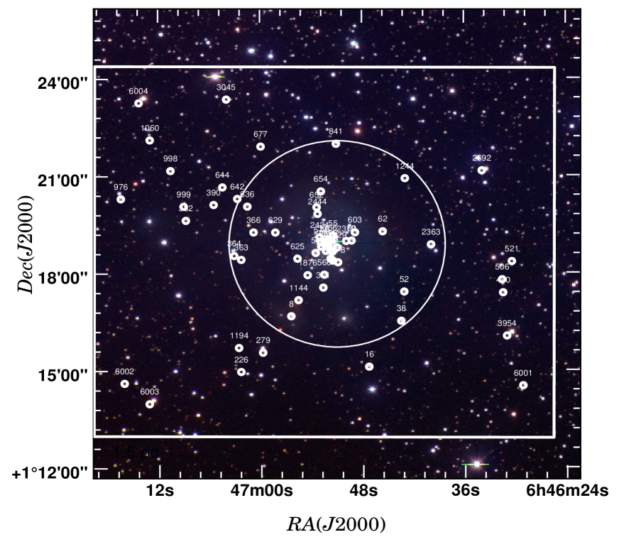
Figure 1: Optical color composite image of NGC 2282 (blue: V; green: R; red: I) obtained at 1.3m DFOT (Up is North, left is East). The cluster area is marked with a large white circle. Our combined monitoring observations were done at the white box region. The variable candidates are marked (see text for details).

Our principal focus of monitoring program is the discovery of rotation periods and characterizing the variability of PMS stars in young clusters. Photometric method to study variable stars is a useful technique to pick up membership against field population in such clusters (e.g., Briceño et al., 2001). It appears as an effective method to identify Weak-line T Tauri Stars (WTTSs) since they are very challenging to be distinguished from the field stars based on their small infrared access. The period distribution in some young clusters (a few Myrs old) is bimodal in the period range 1 to 10 days (Cody & Hillenbrand, 2010; Herbst et al., 2002; Lamm et al., 2005; Coker et al., 2016), while in others bimodality is not present (Makidon et al., 2004). The star-disk connection invokes for such period bimodality (Koenigl, 1991; Shu et al., 1994). The disk locking mechanism was verified by observations on several young clusters from any correlation between the rotation periods and the disk indicators e.g. $\Delta$(I$-$K), $\Delta$(H$-$K_s), [3.6]$-$[8.0] and H$\alpha$ (Edwards et al., 1993; Stassun et al., 1999; Herbst et al., 2002; Makidon et al., 2004; Lamm et al., 2005; Rebull et al., 2006; Cieza & Baliber, 2007; Rodríguez-Ledesma et al., 2010; Cody & Hillenbrand, 2010; Lata et al., 2012). However, no conclusive result was found that those slow rotators are disk-bearing or relatively fast rotators are diskless (Cieza & Baliber, 2007). Review works in this subject area have explored the rotation-disk connection in this low mass end (Herbst et al., 2007; Bouvier, 2007). Mass-rotation connection reveals a clear mass-dependent morphology, which evolves with the ages with relatively fast rotation seen in the low mass end (Irwin et al., 2008; Coker et al., 2016).

NGC 2282 ($\alpha_{2000}$ = $06^{h}46^{m}50.4^{s}$; $\delta_{2000}$ = $+01^{0}18^{m}50^{s}$) is a reflection nebula in the Monoceros constellation, 3 degree away from the Mon OB2 complex and may be associated with it. The cluster parameters of NGC 2282 were first studied by Horner et al. (1997) using NIR data. Subsequently, Dutta et al. (2015) (hereafter Paper I) studied more elaborately the PMS member candidates and cluster parameters of NGC 2282 using deep optical $BVIH\alpha$, UKIDSS $JHK$ and $Spitzer$-IRAC data. Using NIR to MIR color-color (CC) diagram and H$\alpha$-emission, the authors identified 152 PMS member candidates, which include 75 Class II and 9 Class I objects. Majority members are concentrated within the radius of $\sim$ 3.15$\arcmin$, and the minimum extinction towards the region is A_V $\sim$ 1.65 mag. Analyses of the optical and NIR CMDs and disc fraction ($\sim$ 58%), the age of the cluster was determined to be 2 $-$ 5 Myr. Spectroscopic study of bright stars found that the region contains at least three B-type stars. From optical spectroscopic studies, the authors confirmed the previously known main-illuminating source B2V type star, HD 289120, and identified two more high mass stars, one Herbig Ae/Be star (B0.5 Ve) and another B5 V star. From spectroscopy observations, the cluster distance is refined to $\sim$ 1.65 kpc. Thus, NGC 2282 is a suitable object for detailed variability studies as the cluster is relatively populous within a small region, sufficiently nearby and young.

We report here long time-domain photometric studies of NGC 2282 to understand and characterize the variability properties of PMS stars. Section 2 describes with details of our photometric observations including available archival data for the present work. Section 3 contains our result and discussion including analysis of the photometric light curves and identifications of new periodic and aperiodic variable young stars. In this section, we also characterize those periodic variables. Finally, the main results of this work are summarized in section 4.

Table 1: Log of Observations.

Date of	Telescope	I	R	Avg. seeing
Observations		Exp.(s)$\times$ N	Exp.(s)$\times$ N	(arccsec)
15.10.2013	2.0m HCT	60$\times$1, 120$\times$30	200$\times$1	2.5
07.11.2013	2.0m HCT	120$\times$20, 300$\times$ 1	200$\times$1	2.5
08.11.2013	2.0m HCT	120$\times$3, 300$\times$ 1	300$\times$1	2.5
05.01.2014	1.3m DFOT	150$\times$46	250$\times$1	1.8
06.01.2014	1.3m DFOT	150$\times$56	$...$	1.9
29.03.2014	1.3m DFOT	150$\times$49	250 $\times$1	1.75
31.03.2014	1.3m DFOT	150$\times$16, 60$\times$1	250$\times$2, 150$\times$1	1.8
05.10.2014	2.0m HCT	90$\times$2	$...$	1.5
06.10.2014	2.0m HCT	120$\times$2, 90$\times$4, 60$\times$5	$...$	3.2
29.10.2014	2.0m HCT	120$\times$2, 90$\times$5, 60$\times$5	$...$	2.5
30.10.2014	2.0m HCT	120$\times$6, 90$\times$8, 60$\times$3	$...$	2.5
12.11.2014	1.3m DFOT	150$\times$40, 90$\times$27, 60$\times$30	250$\times$2	2.0
13.11.2014	1.3m DFOT	150$\times$25, 90$\times$21, 60$\times$20	250$\times$2	2.0
14.11.2014	1.3m DFOT	150$\times$35, 90$\times$25, 60$\times$25	250$\times$2	2.0
30.11.2014	1.3m DFOT	150$\times$60, 90$\times$41, 60$\times$40	250$\times$2	2.0
01.12.2014	1.3m DFOT	180$\times$60, 90$\times$20, 60$\times$20	250$\times$2	2.0
10.12.2014	1.3m DFOT	180$\times$45, 90$\times$10, 60$\times$10	250$\times$2	2.0
11.12.2014	1.3m DFOT	180$\times$60, 90$\times$15, 60$\times$15	250$\times$2	2.0
12.12.2014	1.3m DFOT	180$\times$50, 90$\times$40, 60$\times$20	250$\times$2	2.0
15.01.2015	2.0m HCT	180$\times$3, 120$\times$4, 60$\times$5	250$\times$2	2.5
16.01.2015	2.0m HCT	120$\times$3, 60$\times$3	200$\times$1	2.5
17.01.2015	2.0m HCT	120$\times$2, 60$\times$2	200$\times$1	2.5
05.10.2015	2.0m HCT	150$\times$2, 60$\times$2	200$\times$1	2.5
07.10.2015	2.0m HCT	300$\times$2, 60$\times$3	200$\times$2	2.5
18.02.2016	2.0m HCT	200$\times$5, 90$\times$6	200$\times$1, 90$\times$1	2.5

2 Data Sets Used

The $RI$ photometric and I-band time-series observations of the cluster NGC 2282 were carried out over 25 epochs during 15 Oct 2013 to 18 Feb 2016 using two different Indian telescopes. We performed photometric observations using the $2048\times 2048$ Andor CCD camera on the 1.3m Devasthal Fast Optical Telescope (DFOT) located at Nainital, India (Sagar et al., 2011). The Andor CCD has a pixel size of 13.5 $\mu$m, which provides a field-of-view (FOV) of about 18$\arcmin$ $\times$ 18$\arcmin$ with a plate-scale of 0.535 arcsec pixel^-1 for F/4 optics of the DFOT. The Andor CCD gain is 6.5 e^-/Analog to Digital Unit(ADU), and the readout noise is 2 e^-. The 2$\times$2 binning observing mode is used to get relatively better signal to noise ratio (SNR). The typical FWHM of the stars were $\sim$ 2$\arcsec$ in our observing run. We also carried out photometric observations using Himalaya Faint Object Spectrograph Camera (HFOSC) on 2m Himalayan Chandra Telescope (HCT) located at Hanle, India (Prabhu, 2014). The $2048\times 2048$ HFOSC imaging CCD provides a FOV of about 10$\arcmin$ $\times$ 10$\arcmin$ with a plate scale of 0.296 arcsec pixel^-1 for F/9 optics of the HCT. The gain of the HFOSC CCD is 1.22 e^-/ADU, and the readout noise is 4.8 e^-. The imaging data is also taken with 2$\times$2 binning mode, and the typical FWHM of the stars were $\sim$ 1.5-3.2$\arcsec$. Long as well as short exposures are taken to get a good dynamical range. The exposure time is decided in such a way that the brighter end is not saturated, and the fainter end has sufficient S/N (uncertainty <0.1). The log of our observations is shown in Table 1. Fig. 1 shows the optical color composite image of NGC 2282, which was taken by the DFOT CCD camera having 18$\arcmin$ $\times$ 18$\arcmin$ FOV, and the HFOSC CCD FOV of 10$\arcmin$ $\times$ 10$\arcmin$ is marked for our overlapping monitoring program.

The photometric reduction of the CCD frames were performed using IRAF software. Using various IRAF tasks, bias correction and flat correction were applied to remove the CCD characteristics and cosmic rays from the raw images. IRAF DAOFIND task is used to detect the point sources in the science frames. Elimination of the extended sources like the background galaxies and brightness enhancements due to bad pixels from the point source catalog was done constraining the roundness limits of $-1$ to $+1$ and the sharpness limits of $0.2$ to $+1$ (Stetson, 1987). The ALLSTAR task of DAOPHOT package is used for PSF photometry (Stetson, 1992). The astrometry on the CCD frames was determined by the IRAF $ccfind$, $ccmap$ and $ccsetwcs$ tasks using the coordinates of 20 isolated moderately bright stars from the 2MASS point source catalog (PSC) (Cutri et al., 2003). Positioning accuracy of better than 0.3$\arcsec$ was obtained.

The available optical to MIR archival data are also used for characterizing the PMS stars of NGC 2282 such as (i) optical $BVI$ data from paper I; (ii) NIR $JHK$ data from the Galactic Plane Survey (GPS; Lucas et al., 2008, data release 6), which were obtained as a part of the UKIRT Infrared Deep Sky Survey (UKIDSS, Lawrence et al., 2007); (iii) the $JHK_{s}$ photometric data from the 2MASS PSC (Cutri et al., 2003) for brighter end (Paper I); (iv) the Spitzer-IRAC observations at 3.6 and 4.5 $\mu$m bands (Program ID: 61071; PI: Whitney, Barbara A) from Paper I; (v) MIR data at 3.4, 4.6, 12, and 22 $\mu$m from the Wide-field Infrared Survey Explorer (WISE) All-sky Survey Data Release (Wright et al., 2010); (vi) the optical data in Sloan broad $r$, $i$ and narrow-band $H\alpha$ filters were obtained from the INT Photometric $H\alpha$ Survey of the Northern Galactic Plane (IPHAS), which was conducted using the Wide Field Camera (WFC) on the 2.5m Isaac Newton Telescope (INT) (Drew et al., 2005; González-Solares et al., 2008; Barentsen et al., 2014).

Figure 2: Example light curves for a few apparently non variable stars of different magnitude range (left three panels) and a few candidate variable stars (right three panels). The $\Delta$m represents the relative magnitude with respect to reference star. Star identifications, $I$ magnitude and RMS value are mentioned. Average error corresponds to each day data is plotted (see text for details).

3 Results and discussion

3.1 Identification of variable stars

3.1.1 Differential Light Curves

Differential photometry was performed to clean the light curves from sky variability, instrument signatures, airmass, etc. We considered a few reference stars in the same CCD frame of the targets, which showed a stable behavior from root-mean-square (RMS) deviation as discussed later and visual inspection of the observed light curve. To obtain relative photometry, we subtract each target star magnitude from those of the reference stars in each frame. The technique of differential photometry provides excellent photometric precision, even in the crowded nebulous region of the cluster. The light curves of a few non-variable and variable stars are displayed in Fig.2. The catalog of detected variable stars from our analysis are listed in Table 2.

Two interesting example light curves are shown in Fig. 3. From the light curves analysis, we identified ID 366 as an eclipsing binary star. Another star ID 2692 shows fast stochastic variability, could be a classical T Tauri candidate as a typical manifestation of the underlying variable accretion processes.

3.1.2 RMS analysis

Considering a large number of sample, one quantitative estimator of photometric variability, i.e., the RMS deviation in the differential photometric light curves is utilized. The mean value of the instrumental magnitudes and the RMS deviation in the light curves were estimated for each star over the whole span of observations for both the telescopes to select the variable stars. Following Carpenter et al. (2001), the observed RMS ($\sigma_{mag}$) for each star was estimated using the following relation as:

$$\sigma^{2}_{mag}=\frac{n\sum_{k=1}^{n}w_{k}(I_{k}-\bar{I})^{2}}{(n-1)\sum_{k=1}^{n}w_{k}},$$ (1)

where $I_{k}$’s are the individual magnitudes associated with photometric uncertainty $\sigma_{k}$’s and weightage $w_{k}=1.0/\sigma_{k}^{2}$ for each observation.

Fig.4 displays the RMS of each star as a function of mean instrumental magnitudes. The RMS of majority stars increases with fainter magnitudes as the signal-to-noise ratio (SNR) decreases towards the fainter limit. The observed RMS values of normal stars follow an expected nearly exponential trend; the RMS values range from $\sim$ 0.01 mag for a brighter end to $\sim$ 0.2 mag towards completeness limit. However, a few stars are scattered from the normal trend. Such type of deviation could be due to the photometric noise or intrinsic variability. From outliers objects in Fig.4, we picked up variable candidates, which are showing RMS equal or more than three times the mean RMS at each half-magnitude bin. We selected 69 variable stars from such criterion. Visual inspection of the light curves indicated that a few of them show large RMS values because of only a few data points, which may be the results of bad pixels, cosmic rays and falling on the edge of the CCD. We rejected those from variable list. Finally, we considered 62 variable candidates for further analysis.

The star-forming history of the young clusters could be probed from the spatial distribution of variable PMS stars. Fig. 1 displays the spatial distribution of the candidate variables towards NGC 2282 (white circles). Majority of the variables are concentrated in the core region of the cluster in the Fig. 1, while a significant scattered population is seen towards the north-east part. Such distribution suggests that the cluster might be extended towards that direction as predicted by Horner et al. (1997).

Figure 3: Example light curves of a eclipsing binary (upper panel) and probably fast stochastic variable (lower panel). All the marks are as Fig. 2 (see text for details).

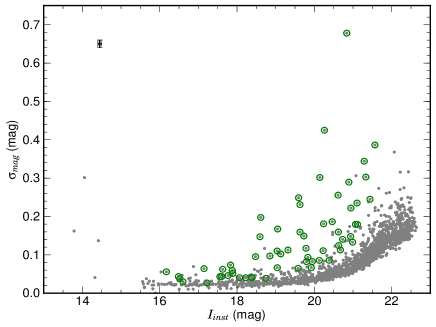
Figure 4: RMS ($\sigma_{mag}$) of the $I_{inst}$-band light curves of 1627 stars towards NGC 2282. The green circles are the candidate variables. The average error bars for magnitudes and rms value are also shown on the top left corner (see text for details).

3.1.3 Period Analysis

The Lomb-Scargle (LS) periodogram analysis (Lomb, 1976; Scargle, 1982) is used to estimate periods of those variable candidates. The LS algorithm is publicly available with the Starlink software package. The LS method is used to find out significant periodicity even with unevenly spaced observed data, and verified successfully in several cases to determine periods from sparse data sets (Lamm et al., 2004; Mondal et al., 2010; Lata et al., 2012). The periods were also verified from other software like PERIOD04, which provides the frequency as well as semi-amplitude of the periodic light curve (Lenz & Breger, 2005). The periods were further verified by online LS periodogram analysis available on NASA Exoplanet Archive Periodogram Service . Out of 62 variable candidates, 41 stars are identified as periodic variables. The LS power spectrum of two variable candidates with identification numbers ID 364 and ID 55 are shown as an example in Figure 5, which show significant periods of 0.546 and 2.309 days, respectively. The significant periods were always verified with visual inspection of the phase light curves and accepted as periodic variables. The periods of variable candidates exhibit in the range 0.233 to 7.143 days and are listed in Table 3. Considering those estimated periods, we generated the phased light curves of variable candidates, and they are presented in Fig. 6.

3.2 Characterization of variable stars

3.2.1 H$\alpha$ Emission property of Variable candidates

The H$\alpha$ emission indicates the young stellar accretion activity in T Tauri phase. Hence this phenomenon could be used to identify the candidate members of the cluster NGC 2282. We made use of the IPHAS archive data as described in section 2 to identify the $H\alpha$ emission variable stars among the variable candidates (see also Paper I). Fig. 7 presents the IPHAS ($r-i/r-H\alpha$) CC diagram of all the candidate variable stars. The nearly vertical green and black lines are the trend of an unreddened optically thick disk continuum and an unreddened Rayleigh-Jeans continuum, respectively (Barentsen et al., 2014). The predicted emission lines with constant EW are shown as the black broken lines. The locus of unreddened main-sequence is represented by the blue lines (solid) and the main-sequence with $-$10 Å  H$\alpha$ emission line (broken), respectively. The stars located above 3$\sigma$ of the main-sequence line having EW $-$10 Å  are considered as Classical T Tauri Stars (CTTSs). However, the identification of CTTSs solely from IPHAS photometry poses difficulty due to the presence of other possible H$\alpha$ emission objects like Be stars, luminous blue variables, interacting binaries, Mira variables, unresolved planetary nebulae, etc.

We identified 21 variable sources as the $H\alpha$ emitting stars from the IPHAS photometry following method as mentioned in the above. We also compared $H\alpha$ emission properties from the IPHAS photometry to that of slitless spectroscopy (Paper I). Rest of the variable stars could be WTTSs with small $H\alpha$ or no $H\alpha$ emission. However, variable $H\alpha$ emission might be a possible reason for such non-detection, even though they emit strong $H\alpha$. The details of the variable candidates having $H\alpha$ emission in NGC 2282 region are listed in Table 3.

3.2.2 NIR Color-Color Diagram

Like H$\alpha$ emission, the NIR excess is a useful diagnostic technique to identify the PMS stars, and such technique is used here to establish the variable candidates as probable PMS objects. We plotted NIR $(J-H)/(H-K)$ CC diagram of the variable candidates in Fig. 8 using $JHK$ data sets as described in section 2. The black solid and long dashed red lines represent the locus of the intrinsic colors of dwarf and giant stars (Bessell & Brett, 1988). The dashed black line is the locus of the CTTSs (Meyer et al., 1997). The intrinsic locus and observed photometric data were transformed into the CIT system following the relations are given by Carpenter (2001). The different interstellar reddening vectors (i.e., $A_{J}$/$A_{V}$ = 0.265, $A_{H}$/$A_{V}$ = 0.155 and $A_{K}$/$A_{V}$ = 0.090) are shown as parallel dashed blue lines, which were adopted from Cohen et al. (1981). The $JHK$ NIR space is divided into F, T, and P sub-regions. The NIR emission of stars in ‘F’ region is believed to originate mainly from their bare photosphere; they might be either the field stars or the WTTSs/Class III sources with small or no NIR excess. The NIR CC diagrams are not sufficient to distinguish between the WTTSs with small NIR excess and the field stars (Ojha et al., 2004). The stars located in the ‘T’ region could be considered as the CTTSs, and they possess optically thick accretion disk (Meyer et al., 1997). This excess emission arises from both photosphere and circumstellar disk (Lada & Adams, 1992). The ‘P’ region stars are considered as protostars, and more NIR color excess at K-band might be originating from the thick envelope or very thick accreting disk around them (Rice et al., 2012).

From Fig.8, we find that majority of the variable stars follow the CTTSs locus. Out of 62 stars, 30 stars (47%) were previously identified as the young stars from either infrared excess, H$\alpha$ emission or both activities. The remaining 32 of 62 variables might be the WTTSs with less IR excess or field stars, and they are located at ‘F’ region in Fig. 8. But spectroscopy follow up is needed to distinguish them from the field stars. However, the YSOs selection in Paper I is still incomplete because of non-availability of longer wavelength data in highly obscured nebulous region.

Figure 5: Example LS power spectrum of selected stars. The highest peaks are considered for period estimation (See text for details).

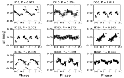
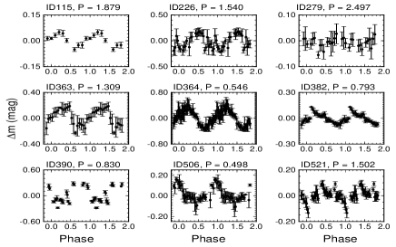
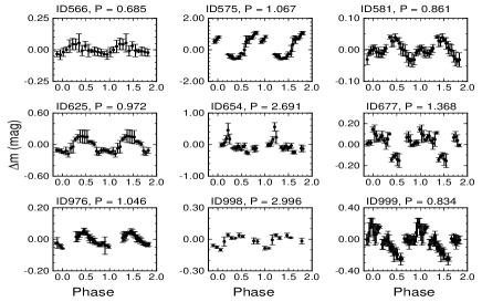
Figure 6: The phase light curve of variables are presented here. Period of variables are taken from Table 3, and the details of the variable IDs are listed in Table 2 (see text for details).

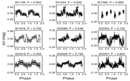
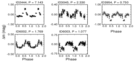
Figure 6: Same as previous figure.

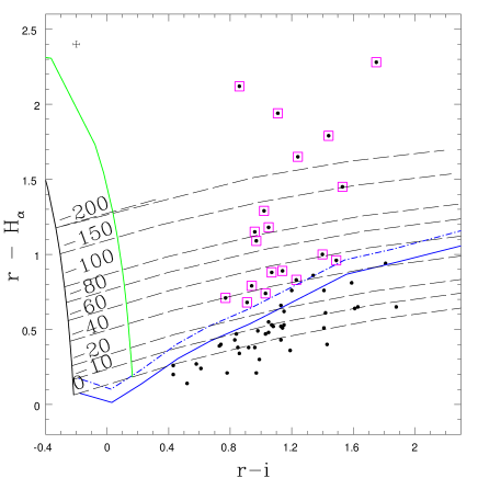
Figure 7: ($r-i$) versus ($r-H\alpha$) CC diagram for all the variable sources detected in the IPHAS catalog towards NGC 2282. The average error bars are also shown on the top left corner. The magenta boxes are the identified H$\alpha$ emission sources from the IPHAS photometry. See text for unreddened continuum and locus of main-sequence and increasing levels of $H\alpha$ emission tracks.

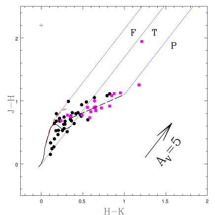
Figure 8: The ($J-H$) versus ($H-K$) CC diagram of variable stars within 3.15$\arcmin$ radius. The magenta filled squares are H$\alpha$ emission objects detected in Fig. 7 and the black filled circles are non-emitting objects. The locus of dwarf (black solid), giants (red long-dashed), CTTSs (black long dashed) and the reddening vectors (blue small dashed) are shown here. The locus for dwarfs and giants are taken from Bessell & Brett (1988), while the locus of CTTSs are adopted from Meyer et al. (1997). The reddening vector of visual extinction $A_{V}$ = 5 mag is also marked. The typical error bars are marked on the top left corner.

3.2.3 Optical Color-Magnitude Diagram of YSOs

The ages and masses of the cluster members could be approximately estimated using the optical CMDs. In Fig. 9, we plotted $V$ vs $(V-I)$ of the PMS variables using the $VI$ data sets from Paper I (see section 2). In Fig. 9, the locus of ZAMS adopted from Girardi et al. (2002) is shown by the dotted curve. The ages and masses of the PMS variables are estimated from the PMS isochrones and evolutionary tracks taken from Bressan et al. (2012), which is plotted in Fig. 9. The PMS isochrones from Siess et al. (2000) are also shown for comparison. The isochrones and evolutionary tracks were corrected considering the cluster distance 1.65 kpc and reddening of $E(V-I)$ = 0.65 mag ($E(B-V)$ = 0.52 mag) (see Sect. 3.3 & 3.4 of Paper I). The reddening vector in CMD space is nearly parallel to the theoretical isochrones. Therefore, a small change in extinction would not show a significant change in the age estimation of the PMSs.

We estimated the masses and ages of the PMS stars using interpolation methods of isochrones and tracks in the CMD compiling $VI$ photometry. Our estimation is limited due to the absence of $V$ measurements of all variable stars. The position of PMS variables in the CMD is spread over 1$-$10 Myr. However, different models at the low-mass end differ significantly as seen in Fig. 9. The average mass of the YSOs seems to be $\sim$ 0.3$-$2.5 M_⊙.

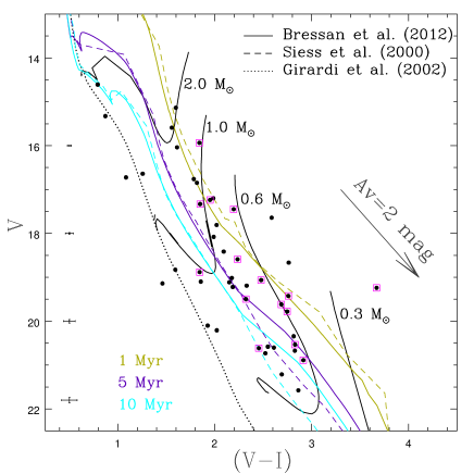
Figure 9: V/(V$-$I) CMD for variable stars towards NGC 2282. All symbols are same as in Fig. 7. The locus of ZAMS adopted from Girardi et al. (2002) is shown as the dotted curve, while the solid lines are the PMS isochrones of age 1.0, 5.0 and 10.0 Myr, respectively. The evolutionary tracks for various mass bins adopted from Bressan et al. (2012) are shown as the thin black solid lines. The average errors in $V$ and ($V-I$) colors are displayed on the left side of the figure.

3.3 Period distribution

All variable stars are searched for periodicity; however, we were managed to estimate periods of $\sim$ 66% stars. Figure 10 displays frequency distribution of rotation periods in NGC 2282. It is to be noted that we have a large number of short-period variables with about 50% and 75% objects having periods less than 1 and 2 days, respectively. We have less number of relatively long (more than 2 days) periodic variables. There are no particular biases for slow or fast rotation periods in our analysis. But, uneven sampling data with long gaps in successive observations without any long single stretch of observations might be a reason to detect a low number of relatively long periodic variables. Again, periodic variability mainly due to spots, which evolve with time and a long gap in data might have masked out such long periods. The period distribution of NGC 2282 is compared with Orion nebula cluster (ONC) stars and NGC 2264 stars with masses greater than 0.25 M_⊙. Herbst et al. (2000, 2002) found a bimodal distribution of the periods for the stars $>$ 0.25 M_⊙ in ONC. But no such conclusive evidence was found for NGC 2264 cluster (Makidon et al., 2004). However, the faint low-mass objects are not covered in their study as NGC 2264 is located at more far distance than ONC. For NGC 2282 stars, the period distribution is unimodal, where fast rotators are peaking up at $\sim$ 0.5-1 days. Hartmann (2002) suggests that the disk locking in highly accreting protostars with smaller magnetosphere have faster rotation periods, and they spin down gradually at the T Tauri phase over the disk braking timescale, which implies that the disk-locking may not be efficient at very early stages in protostars. Herbst et al. (2002), performed a detailed study on ONC, argued that the stars are released from their disk locking after $\sim$ 1 Myr of age. However, Matt & Pudritz (2005) argued that the time scale of disk-locking should be $<$ 4 $\times 10^{4}$ yr. After a comparative study on ONC, Orion Flanking Fields and IC 348, Littlefair et al. (2005) concluded that disk locking takes effect at $\sim$ 1 Myr, and at the age of $\sim$ 3 Myr (IC 348) disk locking is still effective. However, the disk-locking theory could not explain the notable difference of period distribution for NGC 2264 and IC 348. The period distribution of NGC 2282 is strongly biased towards fast rotation side and the lack of slow rotators is quite significant. Our sample mainly consists of stars with periods below four days. This contradiction can be explained by the fact that the size and luminosity of a young star increases dramatically during their rapid accretion phase (e.g. Hartmann & Kenyon, 1996; Kley & Lin, 1999). Hence, the star would appear much younger in the CMD than it’s non-accreting counterpart of the same radius and initial mass (Littlefair et al., 2011). However, some of the results of such period distribution may be effected from cluster environments like variability, extinction, and binarity, etc. (Littlefair et al., 2005, 2011).

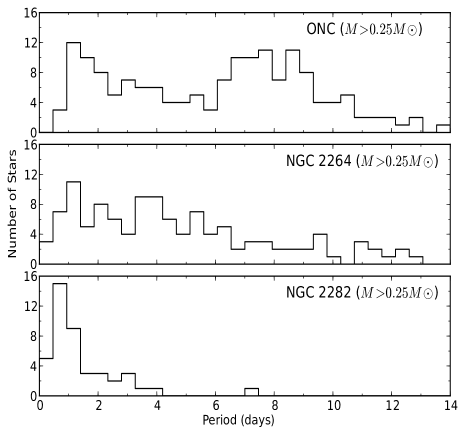
Figure 10: The distribution of periods in NGC 2282 is compared with that of the ONC (Herbst et al., 2002) and NGC 2264 (Makidon et al., 2004). The bimodal period distribution is seen in ONC and NGC 2264, while the distribution for NGC 2282 is uni-modal.

3.4 Correlation between IR excess and rotation periods and variability amplitude

From the time-series photometric observational data on the young (1-5 Myrs) star-forming regions, several authors have investigated any possible correlations between the rotational periods and the presence of circumstellar disks in PMS stars using IR excess and H$\alpha$ emissions. The results reveal significant differences in the rotation periods between stars with circumstellar disks and those lacking disks, and others studies do not find any conclusive evidence (e.g. Rebull, 2001; Herbst et al., 2002; Carpenter et al., 2002; Makidon et al., 2004; Lamm et al., 2005; Rebull et al., 2006; Cieza & Baliber, 2007; Biazzo et al., 2009; Nguyen et al., 2009; Rodríguez-Ledesma et al., 2010; Cody & Hillenbrand, 2010; Rice et al., 2015).

3.4.1 Disk identification

To draw any possible correlation of the NIR excess with rotation rates of our periodic/aperiodic variables, we invoked an index ($I-K$) as defined by Hillenbrand et al. (1998) and subsequently used by several authors (e.g. Herbst et al., 2002; Makidon et al., 2004; Rodríguez-Ledesma et al., 2010). The $I$-band fluxes are believed to be dominated by pure photospheric emission, whereas the $K$-band fluxes have additive circumstellar disk emission on the photospeheric emission (Hillenbrand et al., 1998; Rodríguez-Ledesma et al., 2010). The ($I-K$) index being longer wavelength base provides more pronounce excess compared to other NIR indices (e.g. ($J-H$) or ($H-K$)). The NIR excess from ($I-K$) color defined by Hillenbrand et al. (1998) and the same used by others (e.g. Herbst et al., 2002; Makidon et al., 2004; Rodríguez-Ledesma et al., 2010), can be written as,

$$\Delta(I-K)=(I-K)_{obs}-(A_{I}-A_{K})-(I-K)_{o}$$ (2)

Where is ($I-K$)_obs is the observed magnitudes; A_I and A_K are the interstellar extinctions in $I$ and $K$-bands, respectively. ($I-K$)_o is the intrinsic color of the star. Without knowledge of spectral types, the intrinsic color is difficult to measure, and this is the case for our variables. However, it could be estimated from photometric measurements, extinction, and theoretical isochrones. Following Rodríguez-Ledesma et al. (2010), first, we measured the intrinsic colors ($I-J$)_o as it is expected to be originating from photospheric emission from observed ($I-J$) colors corrected by the average extinction of A_v = 1.65 mag (see Paper I). Using the Baraffe et al. (1998) color information of NGC 2282 and the mean age of 3 Myrs (Paper I), we estimated the intrinsic color ($I-K$)_o from ($I-J$)_o. The NIR excess $\Delta(I-K)$ are calculated using Eqn. 2 for individual variables. It is to be noted that intrinsic color estimation of the young stars by comparing the observational data with the theoretical isochrones of mean age corrected for average extinction is an unrealistic approach, which includes several errors from nonuniform extinction, excess disk emission, variability, and binarity. However, it provides indicative results for further observations.

To search possible correlation between the rotation rates and the NIR excess we have plotted period versus $\Delta(I-K)$. Following Herbst et al. (2002); Makidon et al. (2004); Rodríguez-Ledesma et al. (2010), the value of $\Delta(I-K)$ = 0.3 mag is adopted for separating the disk and disk-less stars. Out of 41 periodic variables, we don’t have K-band measurements for two objects. We plotted 39 periodic variables in the upper panel of Fig.11 (upper panel), where 16 objects show NIR excess in $\Delta(I-K)$. We have 15 H$\alpha$ emitting periodic variables that are marked in Fig 11. These H$\alpha$ emitting sources are selected from IPHAS photometry (see sec. 3.2.1). NIR excess indicates the presence of near-photospheric circumstellar dust, while H$\alpha$ emission is a good indicator of accretion in T-Tauri stars. Out of 16 NIR excess sources, 10 objects exhibit H$\alpha$ emission. We obtained disk fraction of about 41% among periodic variables from the NIR excess analysis. Since we have longer wavelengths Spitzer data in IRAC bands 3.6 and 4.5 $\micron$ for NGC 2282 as mentioned in sec. 2 (see also Paper I), these could be used for probing better disk indicator than NIR wavelengths (Lada et al., 2000; Rodríguez-Ledesma et al., 2010; Jose et al., 2017). However, nebular PAH emission on the central part of the cluster might be problematic sometimes at IRAC bands (Gutermuth et al., 2009). Among 41 periodic variables, 33 have MIR data. In the lower panel of Fig.11, we plotted the period versus $Spitzer$-IRAC (see. section 2) color [3.6] -[4.5] for all 33 variables. The population of variables close to [3.6] -[4.5]$\approx$ 0 indicates diskless bare photospheric color (Patten et al., 2006). The colors [3.6] -[4.5] $>$ 0.7 and $>$0.15 indicate Class I and Class II sources respectively (Gutermuth et al., 2008; Gutermuth et al., 2009). We adopt conservatively the color [3.6] -[4.5] $>$ 0.25 criterion for the disked stars as shown in Fig.11 (lower panel). We obtained relatively higher disk fraction of $\sim$51% based on MIR data. This is comparable to the disk fraction estimation in Paper I ($\sim$58%) for all the PMS sources within NGC 2282.

3.4.2 Rotation/variability amplitude to disk connection

To understand rotation-disk connection in our periodic variables, the IR excesses versus periods are plotted in Fig.11. The disk-locking system should have relatively longer periods as compared to that of diskless stars as studied before in the literature. In Fig.11, the few disked stars have a larger range of periods whereas the few slow rotators also have disks around them. This finding could be related to the age of NGC 2282, as it is relatively old (2$-$3 Myrs), and such disk-locking systems may be efficient at the young age of $\sim$ 1 Myr or less as suggested by several authors and already described in earlier section 3.3. However, we are unable to draw any conclusion about disk-locking theory due to our statistically small number of samples.

We also analyzed whether there is any correlation between variability amplitude of the periodic/aperiodic variables and the IR excess using $\Delta(I-K)$ and [3.6]-[4.5] as stated in the above section. We have total 62 variables, and 51 have both [3.6] and [4.5] measurements. In Fig. 12, we plotted the variability amplitude from the light curve RMS versus NIR excess $\Delta(I-K)$ (upper panel) and MIR excess [3.6]-[4.5] (lower panel). A trend of increasing variability amplitude with IR excess is seen in Fig.12. Such results suggest that the objects with thick circumstellar disk tend to have relatively larger light-curve amplitudes. Thus, the presence of thick disk around stars preferably display variable phenomena due to their accretion activity.

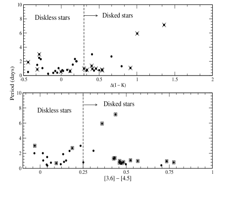
Figure 11: Periods are plotted as a function of disk indicator NIR excess $\Delta(I-K)$ (upper panel) and MIR excess [3.6]$-$[4.5] (lower panel) for periodic variables. The vertical solid lines of $\Delta(I-K)$ = 0.3 and [3.6]$-[$4.5]=0.25 are adopted as the boundary of diskless and disked stars. In upper panel, the H$\alpha$ emitting sources are marked by the cross symbols. In lower panel, NIR excess sources are marked by the squares. No conclusive trends are seen in the plots for disk-locking mechanism.

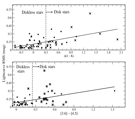
Figure 12: The light curves RMS (variability amplitude) are plotted as a function of disk indicator NIR excess $\Delta(I-K)$ (upper panel) and MIR excess [3.6]$-$[4.5] (lower panel) for periodic and aperiodic variables. The vertical dotted lines of $\Delta(I-K)$ = 0.3 and [3.6]$-$[4.5]=0.25 are adopted as the boundary of diskless and disked stars. In the upper panel, the H$\alpha$ emitting sources are marked by the cross symbols. In the lower panel, NIR excess sources are marked by the open squares. The dashed line obeys a clear increasing trend of RMS with infrared excess.

3.5 Period-mass correlation

To investigate any correlation between the rotation periods and the masses, we have plotted the rotation periods versus stellar masses for periodic variables in NGC 2282 in Fig.13. The masses are estimated from I-band magnitudes and the mean cluster extinction (A_v=1.65 mag), based on the 3 Myr theoretical isochrones of Baraffe et al. (1998). The estimated masses range from 0.1 M$\odot$ to 2.5 M$\odot$. The mass estimation based on the isochrones is quite uncertain at these young ages. Furthermore, the lower mass limit of 0.1 M$\odot$ lies near to I$\sim$ 20.5 mag, where the light curves do not have sufficient precision to detect any variability due to poor SNR at such faint end. For comparison, we plotted the period distribution with masses in NGC 2362 ($\sim$5 Myr), taken from Irwin et al. (2008). From Fig.13, it is apparent that the rotation period follows a flat to sloping mass dependence of the rotation periods in NGC 2282 ($\sim$3 Myr). However, our periodic variables detection is not sensitive enough at the lower mass close to 0.3 M$\odot$, and hence the result has to be taken with caution. Furthermore, we suspect that the mass determinations might be unreliable due to spatial variable extinction in the cluster area. Such variable extinction introduces horizontal dispersion in the mass versus period plot. Lack of spectroscopy on such individual low-mass objects, the proper value of extinction may be unreliable from photometry only, and we prefer to use the mean extinction to estimate masses here. It is worth to point out that by adopting variable extinction values in the individual cluster members would cause the changes in the stellar masses 25 $-$ 40% of our estimated values.

Our result agrees with the correlation of gradual evolutionary sequence; no mass dependence with the rotation periods at the younger cluster to the mass dependent rotation rates at the older cluster (e.g. Irwin et al., 2008; Coker et al., 2016, and references therein). Fig. 12 of Irwin et al. (2008) shows no-mass dependency relation to the rotation periods in the ONC ($\sim$1 Myr). While a weak-mass dependency (fast rotation at the low-mass stars compared to that of high-mass stars) relation is seen in NGC 2264 ($\sim$2 Myr) and 2362($\sim$5 Myr), and a strong-mass dependency in more older clusters NGC 2547 ($\sim$40 Myr) and NGC 2516 ($\sim$150 Myr).

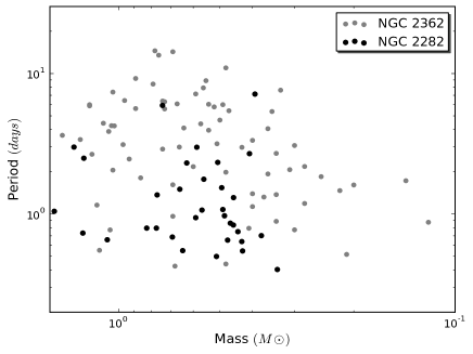
Figure 13: Mass versus period is plotted for periodic variables in the mass range $\sim$0.25$-$1.6 M_⊙. From our detection limit, periodic variables are identified up to the low mass limit of $\geq$ 0.25 M_⊙, and a systematic trend for fast rotators at the low mass-end might be real feature as seen in other a few regions (see Irwin et al., 2008)

4 Summary and Conclusions

In this paper, we present deep $I$-band ($\sim$ 20.5 mag) long-term photometric monitoring studies of the stars towards a young (2$-$5 Myr) cluster NGC 2282 in the Monoceros constellation to understand the variability characteristics towards the low-mass end of PMS stars. Our main results are summarized as follows:

1. From the differential photometry light curves of 1627 stars, we have identified 62 new photometric variable stars. Out of 62 variables, 41 are periodic variables and yield the rotation periods from 0.2 to 7 days.

2. Based on the H$\alpha$ emission activities, J$-$H/H$-$K CC diagram, IR excess, and paper I, we found the majority of the variable stars are members of the cluster.

3. The period distribution shows a median period of $\sim$1 day as seen in other young clusters (e.g., NGC 2264, ONC, etc.). It displays a unimodal distribution like others; but younger clusters like the ONC have bimodal distribution with slow rotators peaking at $\sim$ 6$-$8 days.

4. To understand the disk-locking hypothesis in young PMS though rotation-disk connection, we derived NIR excess from $\Delta$(I$-$K) and MIR excess from $Spitzer$ [3.6]$-$[4.5] $\mu$m data. No conclusive correlation of slow rotation with the presence of disks around stars and fast rotation for diskless stars is seen from the periodic variables in NGC 2282.

5. Furthermore, to investigate the variability-disk connection, we studied NIR excess, and MIR excess from $Spitzer$ data with the variability amplitude (RMS) derived from the light curves. A clear increasing trend of variability amplitude with IR excess is seen for all the periodic/aperiodic variables.

6. Disk fraction among the periodic variables are studied using NIR and MIR excess as discussed, we estimated the fraction of $\sim$51% for all the periodic/aperiodic variables, while $\sim$41% for periodic variables. This estimation is comparable to the disk fraction ($\sim$58%) obtained for the entire PMS population in Paper I.

7. To understand fast rotation in the lower mass end of the PMS stars, the period-mass correlation in the mass range 0.3$-$1.6 M_⊙ is studied. It is apparent from our analysis that there is an evidence of relatively fast rotation with decreasing masses (sloping relation) as seen in the literature (Irwin et al., 2008; Coker et al., 2016). However, our periodic variables selection is not sensitive enough at the lower mass beyond 0.3 M_⊙, and hence the results need to be taken with caution.

Table 2: Catalog of the identified variable stars. The complete table is available in the electronic version.

ID	$\alpha_{2000}$	$\delta_{2000}$	$B$	$V$	$R$	$I$	$J$	$H$	$K$	3.6 $\mu$m	4.5 $\mu$m	W1	W2
	(deg)	(deg)	(mag)	(mag)	(mag)	(mag)	(mag)	(mag)	(mag)	(mag)	(mag)	(mag)	(mag)
8	101.735121	1.277934	16.971	15.934	14.935	14.189	12.061	11.212	10.572	9.616	9.049	4.189	1.079
			$\pm$ 0.012	$\pm$ 0.013	$\pm$ 0.007	$\pm$ 0.003	$\pm$ 0.023	$\pm$ 0.020	$\pm$ 0.023	$\pm$ 0.003	$\pm$ 0.002	$\pm$ 0.015	$\pm$ 0.021
16	101.697027	1.251858	17.546	16.037	15.260	14.314	12.930	12.423	12.075	12.083	99.999	10.109	7.073
			$\pm$ 0.049	$\pm$ 0.043	$\pm$ 0.039	$\pm$ 0.046	$\pm$ 0.026	$\pm$ 0.034	$\pm$ 0.034	$\pm$ 0.004	$\pm$99.999	$\pm$ 0.092	$\pm$ 0.160
38	101.681203	1.275360	15.257	14.608	14.147	13.876	13.306	12.956	12.952	12.842	12.826	9.541	7.619
			$\pm$ 0.007	$\pm$ 0.008	$\pm$ 0.009	$\pm$ 0.005	$\pm$ 0.030	$\pm$0.001	$\pm$ 0.044	$\pm$ 0.008	$\pm$ 0.009	$\pm$ 0.093	$\pm$ 0.203
52	101.679695	1.290380	19.691	17.640	16.207	14.898	12.795	11.770	11.406	11.121	11.154	11.955	8.283
			$\pm$ 0.020	$\pm$ 0.004	$\pm$ 0.009	$\pm$ 0.006	$\pm$ 0.020	$\pm$ 0.026	$\pm$ 0.023	$\pm$ 0.003	$\pm$ 0.004	$\pm$99.999	$\pm$99.999
53	101.715712	1.307466	16.823	15.588	14.729	13.999	12.775	12.126	11.936	11.688	11.646	6.786	3.643
			$\pm$ 0.008	$\pm$ 0.004	$\pm$ 0.007	$\pm$ 0.003	$\pm$ 0.026	$\pm$ 0.028	$\pm$ 0.030	$\pm$ 0.004	$\pm$ 0.005	$\pm$99.999	$\pm$ 0.119
54	101.723024	1.310400	18.770	17.447	16.363	17.674	13.677	12.644	11.958	10.761	10.026	99.999	99.999
			$\pm$ 0.013	$\pm$ 0.005	$\pm$ 0.009	$\pm$ 0.009	$\pm$ 0.026	$\pm$ 0.026	$\pm$ 0.027	$\pm$ 0.003	$\pm$ 0.002	$\pm$99.999	$\pm$99.999
55	101.714484	1.319228	99.999	16.760	16.161	17.549	13.439	12.624	12.409	12.229	12.058	99.999	99.999
			$\pm$99.999	$\pm$ 0.072	$\pm$ 0.008	$\pm$ 0.020	$\pm$ 0.036	$\pm$ 0.027	$\pm$ 0.033	$\pm$ 0.004	$\pm$ 0.006	$\pm$99.999	$\pm$99.999
58	101.718528	1.316127	16.417	15.134	14.292	13.575	12.280	11.593	11.379	11.219	11.139	99.999	99.999
			$\pm$ 0.014	$\pm$ 0.011	$\pm$ 0.012	$\pm$ 0.004	$\pm$ 0.029	$\pm$ 0.033	$\pm$ 0.033	$\pm$ 0.003	$\pm$ 0.004	$\pm$99.999	$\pm$99.999

• N.B. The value ‘99.999’ represent the absence of the particular magnitude.

Table 3: Result of our analysis : periods, membership characteristics, IR excess, masses of the identified variable stars.

ID	I*	Ierr	RMS	H$\alpha$**	Period	PMS from Paper I	$\Delta$(I$-$K)	[3.6]$-$[4.5]	mass***
	(mag)	(mag)	(mag)	(emission Y/N)	(days)	(Yes/No)	(mag)	(mag)	(M⊙)
8	14.189	0.003	0.043	Y	0.972	Yes	0.300	0.567	2.43
16	14.314	0.046	0.064	N	0.254	No	-0.174	$...$	2.33
38	13.876	0.005	0.038	N	2.011	No	0.197	0.016	2.69
52	14.898	0.006	0.043	N	2.003	No	0.202	-0.033	1.90
53	13.999	0.003	0.03	N	0.373	No	-0.106	0.042	2.58
54	17.674	0.009	0.046	Y	0.942	Yes	0.410	0.735	0.59
55	17.549	0.02	0.043	N	2.309	No	-0.271	0.171	0.63
58	13.575	0.004	0.056	N	$...$	No	-0.085	0.08	2.96
60	15.274	0.005	0.059	N	1.039	No	-0.036	0.151	1.66
62	14.979	0.004	0.062	N	0.754	No	0.013	0.063	1.84
115	15.27	0.008	0.052	Y	1.879	Yes	-0.438	0.134	1.66
226	18.026	0.058	0.148	N	1.540	No	0.152	$...$	0.49
279	15.965	0.009	0.04	N	2.497	No	-0.293	$...$	1.27
321	16.448	0.008	0.249	N	$...$	Yes	1.030	0.44	1.04
363	18.182	0.025	0.14	N	1.309	Yes	0.797	0.427	0.45
364	18.299	0.044	0.289	N	0.546	Yes	0.114	0.498	0.43
366	17.17	0.015	0.082	N	$...$	No	-0.054	0.15	0.75
382	16.968	0.012	0.065	N	0.794	Yes	0.077	0.251	0.82
390	17.202	0.013	0.181	Y	5.930	Yes	1.003	0.36	0.74
480	15.747	0.007	0.042	N	$...$	No	-0.122	0.087	1.38
506	17.956	0.028	0.086	N	0.499	No	-0.439	0.038	0.51
521	17.451	0.02	0.082	N	1.502	No	-0.318	0.041	0.65
566	17.345	0.021	0.067	N	0.686	No	0.333	0.094	0.69
571	16.35	0.01	0.097	Y	$...$	Yes	0.546	0.392	1.08
575	17.76	0.021	0.425	Y	1.066	Yes	0.914	0.525	0.56
578	19.061	0.026	0.113	Y	$...$	Yes	0.132	0.393	0.28
581	18.14	0.016	0.04	Y	0.861	Yes	-0.317	0.139	0.46
603	16.54	0.009	0.11	Y	$...$	Yes	0.683	0.571	0.99
625	18.063	0.028	0.16	Y	0.972	Yes	0.459	0.462	0.48
629	17.367	0.018	0.149	Y	$...$	Yes	0.363	0.436	0.68
636	16.062	0.009	0.039	N	$...$	No	-0.069	0.052	1.22
642	17.178	0.013	0.117	N	$...$	No	0.115	0.127	0.75
644	17.396	0.018	0.302	Y	$...$	Yes	1.597	0.557	0.67
652	16.584	0.01	0.167	N	$...$	Yes	0.142	0.136	0.98
654	18.388	0.025	0.344	N	2.690	Yes	0.663	0.187	0.41
677	17.123	0.015	0.159	Y	1.368	Yes	0.401	0.434	0.77
841	14.575	0.004	0.027	N	$...$	No	-0.037	-0.06	2.13
976	15.449	0.007	0.04	N	1.046	No	-0.249	0.018	1.55
998	15.796	0.02	0.095	N	2.996	No	0.406	-0.031	1.35
999	18.18	0.04	0.133	Y	0.835	Yes	0.538	0.484	0.45
1060	16.859	0.013	0.231	N	$...$	Yes	0.247	0.209	0.86
1144	16.113	0.037	0.197	Y	$...$	Yes	2.014	$...$	1.19
1194	18.104	0.062	0.179	N	0.652	No	0.024	$...$	0.47
1244	18.289	0.047	0.179	N	0.637	No	-0.080	$...$	0.43
1366	17.689	0.045	0.073	Y	2.989	Yes	-0.292	0.235	0.58
1876	18.539	0.048	0.386	N	0.702	No	0.432	0.475	0.37
2286	17.492	0.032	0.086	Y	0.549	Yes	-0.004	0.12	0.64
2301	17.914	0.04	0.256	N	$...$	Yes	-0.043	0.599	0.52
2303	15.948	0.047	0.147	Y	0.732	Yes	0.541	0.461	1.27
2319	18.739	0.045	0.245	N	0.403	No	-0.053	0.704	0.34
2329	17.112	0.028	0.093	Y	0.794	Yes	0.339	0.776	0.77
2337	16.353	0.007	0.066	Y	0.656	Yes	0.116	0.471	1.08
2363	17.762	0.01	0.186	N	$...$	No	-0.093	0.013	0.56
2424	19.398	0.143	0.303	N	$...$	No	-0.094	1.534	0.23
2444	18.458	0.041	0.678	Y	7.143	Yes	1.359	0.438	0.39
2692	16.681	0.019	0.102	N	$...$	No	-0.151	0.024	0.94
3045	17.973	0.033	0.113	N	2.331	Yes	0.180	0.31	0.51
3954	18.239	0.088	0.235	N	0.749	No	0.501	$...$	0.44
6001	15.348	0.008	0.043	N	$...$	No	-0.210	$...$	1.61
6002	17.785	0.026	0.111	N	1.769	No	$...$	$...$	0.56
6003	18.041	0.067	0.222	N	1.077	No	$...$	$...$	0.49
6004	17.744	0.046	$...$	N	$...$	No	$...$	$...$	0.57

• Mean $I$ magnitude from the light curve.
  

• From IPHAS photometry. See text for details.
  

• From I magnitude, mean extinction and theoretical isochrones of 3 Myr from Baraffe et al. (1998)

References

- Baraffe et al. (1998) Baraffe I., Chabrier G., Allard F., Hauschildt P. H., 1998, A&A, 337, 403
- Barentsen et al. (2014) Barentsen G., et al., 2014, MNRAS, 444, 3230
- Bessell & Brett (1988) Bessell M. S., Brett J. M., 1988, PASP, 100, 1134
- Biazzo et al. (2009) Biazzo K., Melo C. H. F., Pasquini L., Randich S., Bouvier J., Delfosse X., 2009, A&A, 508, 1301
- Bouvier (2007) Bouvier J., 2007, in Bouvier J., Appenzeller I., eds, IAU Symposium Vol. 243, Star-Disk Interaction in Young Stars. pp 231–240 (arXiv:0712.2988), doi:10.1017/S1743921307009593
- Bressan et al. (2012) Bressan A., Marigo P., Girardi L., Salasnich B., Dal Cero C., Rubele S., Nanni A., 2012, MNRAS, 427, 127
- Briceño et al. (2001) Briceño C., et al., 2001, Science, 291, 93
- Briceño et al. (2005) Briceño C., Calvet N., Hernández J., Vivas A. K., Hartmann L., Downes J. J., Berlind P., 2005, AJ, 129, 907
- Carpenter (2001) Carpenter J. M., 2001, AJ, 121, 2851
- Carpenter et al. (2001) Carpenter J. M., Hillenbrand L. A., Skrutskie M. F., 2001, AJ, 121, 3160
- Carpenter et al. (2002) Carpenter J. M., Hillenbrand L. A., Skrutskie M. F., Meyer M. R., 2002, AJ, 124, 1001
- Cieza & Baliber (2007) Cieza L., Baliber N., 2007, ApJ, 671, 605
- Cody & Hillenbrand (2010) Cody A. M., Hillenbrand L. A., 2010, ApJS, 191, 389
- Cohen et al. (1981) Cohen J. G., Persson S. E., Elias J. H., Frogel J. A., 1981, ApJ, 249, 481
- Cohen et al. (2004) Cohen R. E., Herbst W., Williams E. C., 2004, AJ, 127, 1602
- Coker et al. (2016) Coker C. T., Pinsonneault M., Terndrup D. M., 2016, ApJ, 833, 122
- Cutri et al. (2003) Cutri R. M., et al., 2003, 2MASS All Sky Catalog of point sources.
- Drew et al. (2005) Drew J. E., et al., 2005, MNRAS, 362, 753
- Dutta et al. (2015) Dutta S., Mondal S., Jose J., Das R. K., Samal M. R., Ghosh S., 2015, MNRAS, 454, 3597
- Edwards et al. (1993) Edwards S., et al., 1993, AJ, 106, 372
- Girardi et al. (2002) Girardi L., Bertelli G., Bressan A., Chiosi C., Groenewegen M. A. T., Marigo P., Salasnich B., Weiss A., 2002, A&A, 391, 195
- González-Solares et al. (2008) González-Solares E. A., et al., 2008, MNRAS, 388, 89
- Gutermuth et al. (2008) Gutermuth R. A., et al., 2008, ApJ, 674, 336
- Gutermuth et al. (2009) Gutermuth R. A., Megeath S. T., Myers P. C., Allen L. E., Pipher J. L., Fazio G. G., 2009, ApJS, 184, 18
- Hartmann (2002) Hartmann L., 2002, ApJ, 566, L29
- Hartmann & Kenyon (1996) Hartmann L., Kenyon S. J., 1996, ARA&A, 34, 207
- Herbig (1962) Herbig G. H., 1962, Advances in Astronomy and Astrophysics, 1, 47
- Herbst et al. (1994) Herbst W., Herbst D. K., Grossman E. J., Weinstein D., 1994, AJ, 108, 1906
- Herbst et al. (2000) Herbst W., Rhode K. L., Hillenbrand L. A., Curran G., 2000, AJ, 119, 261
- Herbst et al. (2002) Herbst W., Bailer-Jones C. A. L., Mundt R., Meisenheimer K., Wackermann R., 2002, A&A, 396, 513
- Herbst et al. (2007) Herbst W., Eislöffel J., Mundt R., Scholz A., 2007, Protostars and Planets V, pp 297–311
- Hillenbrand et al. (1998) Hillenbrand L. A., Strom S. E., Calvet N., Merrill K. M., Gatley I., Makidon R. B., Meyer M. R., Skrutskie M. F., 1998, AJ, 116, 1816
- Horner et al. (1997) Horner D. J., Lada E. A., Lada C. J., 1997, AJ, 113, 1788
- Irwin et al. (2008) Irwin J., Hodgkin S., Aigrain S., Bouvier J., Hebb L., Irwin M., Moraux E., 2008, MNRAS, 384, 675
- Joergens et al. (2003) Joergens V., Fernández M., Carpenter J. M., Neuhäuser R., 2003, ApJ, 594, 971
- Jose et al. (2017) Jose J., Herczeg G. J., Samal M. R., Fang Q., Panwar N., 2017, ApJ, 836, 98
- Joy (1945) Joy A. H., 1945, ApJ, 102, 168
- Kley & Lin (1999) Kley W., Lin D. N. C., 1999, ApJ, 518, 833
- Koenigl (1991) Koenigl A., 1991, ApJ, 370, L39
- Lada & Adams (1992) Lada C. J., Adams F. C., 1992, ApJ, 393, 278
- Lada et al. (2000) Lada C. J., Muench A. A., Haisch Jr. K. E., Lada E. A., Alves J. F., Tollestrup E. V., Willner S. P., 2000, AJ, 120, 3162
- Lamm et al. (2004) Lamm M. H., Bailer-Jones C. A. L., Mundt R., Herbst W., Scholz A., 2004, A&A, 417, 557
- Lamm et al. (2005) Lamm M. H., Mundt R., Bailer-Jones C. A. L., Herbst W., 2005, A&A, 430, 1005
- Lata et al. (2012) Lata S., Pandey A. K., Chen W. P., Maheswar G., Chauhan N., 2012, MNRAS, 427, 1449
- Lawrence et al. (2007) Lawrence A., et al., 2007, MNRAS, 379, 1599
- Lenz & Breger (2005) Lenz P., Breger M., 2005, Communications in Asteroseismology, 146, 53
- Littlefair et al. (2005) Littlefair S. P., Dhillon V. S., Martín E. L., 2005, A&A, 437, 637
- Littlefair et al. (2011) Littlefair S. P., Naylor T., Mayne N. J., Saunders E., Jeffries R. D., 2011, MNRAS, 413, L56
- Lomb (1976) Lomb N. R., 1976, Ap&SS, 39, 447
- Lucas et al. (2008) Lucas P. W., et al., 2008, MNRAS, 391, 136
- Makidon et al. (2004) Makidon R. B., Rebull L. M., Strom S. E., Adams M. T., Patten B. M., 2004, AJ, 127, 2228
- Matt & Pudritz (2005) Matt S., Pudritz R. E., 2005, MNRAS, 356, 167
- Meyer et al. (1997) Meyer M. R., Calvet N., Hillenbrand L. A., 1997, AJ, 114, 288
- Mondal et al. (2010) Mondal S., et al., 2010, AJ, 139, 2026
- Nguyen et al. (2009) Nguyen D. C., Jayawardhana R., van Kerkwijk M. H., Brandeker A., Scholz A., Damjanov I., 2009, ApJ, 695, 1648
- Ojha et al. (2004) Ojha D. K., et al., 2004, ApJ, 608, 797
- Patten et al. (2006) Patten B. M., et al., 2006, ApJ, 651, 502
- Prabhu (2014) Prabhu T. P., 2014, Proceedings of the Indian National Science Academy Part A, 80, 887
- Rebull (2001) Rebull L. M., 2001, AJ, 121, 1676
- Rebull et al. (2006) Rebull L. M., Stauffer J. R., Megeath S. T., Hora J. L., Hartmann L., 2006, ApJ, 646, 297
- Rice et al. (2012) Rice T. S., Wolk S. J., Aspin C., 2012, ApJ, 755, 65
- Rice et al. (2015) Rice T. S., Reipurth B., Wolk S. J., Vaz L. P., Cross N. J. G., 2015, AJ, 150, 132
- Rodríguez-Ledesma et al. (2010) Rodríguez-Ledesma M. V., Mundt R., Eislöffel J., 2010, A&A, 515, A13
- Sagar et al. (2011) Sagar R., et al., 2011, Current Science, 101, 1020
- Scargle (1982) Scargle J. D., 1982, ApJ, 263, 835
- Scholz & Eislöffel (2004) Scholz A., Eislöffel J., 2004, A&A, 419, 249
- Shu et al. (1994) Shu F., Najita J., Ostriker E., Wilkin F., Ruden S., Lizano S., 1994, ApJ, 429, 781
- Siess et al. (2000) Siess L., Dufour E., Forestini M., 2000, A&A, 358, 593
- Stassun et al. (1999) Stassun K. G., Mathieu R. D., Mazeh T., Vrba F. J., 1999, AJ, 117, 2941
- Stetson (1987) Stetson P. B., 1987, PASP, 99, 191
- Stetson (1992) Stetson P. B., 1992, in Worrall D. M., Biemesderfer C., Barnes J., eds, Astronomical Society of the Pacific Conference Series Vol. 25, Astronomical Data Analysis Software and Systems I. p. 297
- Wright et al. (2010) Wright E. L., et al., 2010, AJ, 140, 1868