Scalar products of the elliptic Felderhof model
and elliptic Cauchy formula

Abstract

We analyze the scalar products of the elliptic Felderhof model introduced by Foda-Wheeler-Zuparic as an elliptic extension of the trigonometric face-type Felderhof model by Deguchi-Akutsu. We derive the determinant formula for the scalar products by applying the Izergin-Korepin technique developed by Wheeler to investigate the scalar products of integrable lattice models. By combining the determinant formula for the scalar products with the recently-developed Izergin-Korepin technique to analyze the wavefunctions, we derive a Cauchy formula for elliptic Schur functions.

Elliptic integrable models are classes of integrable models described by elliptic functions. Investigations of elliptic integrable models lead to new discoveries of mathematical structures. An instance is the notion of elliptic quantum groups [1, 2, 3, 4] which are extensions of the quantum groups [5, 6, 7], introduced through the analysis of the eight-vertex model, eight-vertex solid-on-solid model and their generalizations [8, 9, 10, 11, 12]. Recently, there are also progresses on partition functions of the eight-vertex solid-on-solid models [13, 14, 15, 16, 17, 18, 19, 20, 21, 22, 23, 24, 25, 26] from the viewpoint of the quantum inverse scattering method [27, 28], vertex operator method [29] and so on.

In this paper, we investigate another class of elliptic integrable model. We analyze the scalar products of the elliptic Felderhof model introduced by Foda-Wheeler-Zuparic [30] as an extension of the face-type Felderhof model [31] by Deguchi-Akutsu [32]. The elliptic Felderhof model (Foda-Wheeler-Zuparic model), and its closely related elliptic Perk-Schultz model (Okado-Deguchi-Fujii-Martin model) constructed by Okado [33], Deguchi-Fujii [34] and Deguchi-Martin [35] as an elliptic extension of the Perk-Schultz model [36], are interesting models to be investigated, since the corresponding trigonometric models were discovered by number theorists recently to be related with automorphic representation theory and deformations of Weyl character formulas (Tokuyama formulas) for symmetric functions. Bump-Brubaker-Friedberg [37] constructed free-fermion models by themselves and showed that the wavefunctions are given as a product of a deformed Vandermonde determinant and Schur functions. One of the consequences of their results is the natural construction of the Tokuyama formula [38] as wavefunctions of integrable models, which is a one-parameter deformation of the Weyl character formula for the Schur functions. Their result is the one of the main motivations to study the elliptic Felderhof model of Foda-Wheeler-Zuparic and the elliptic Perk-Schultz model of Okado, Deguchi-Fujii and Deguchi-Martin, since these models can be regarded as elliptic analogues of the free-fermion model which Bump-Brubaker-Friedberg introduced and analyzed (the quantum group structure of the trigonometric models can be found in [32, 39, 40] for example) . There are not so much studies on the partition functions of these elliptic models. Foda-Wheeler-Zuparic showed the factorization of the domain wall boundary partition functions of these models [30] by applying the Izergin-Korepin technique [41, 42], which is a classical method to analyze the domain wall boundary partition functions of integrable models. Recently, we extended the Izergin-Korepin technique to be able to anlayze the wavefunctions [43, 44, 45], and showed that the wavefunctions of these elliptic models are given as a deformed elliptic Vandermonde determinant and elliptic symmetric functions which can be viewed as elliptic Schur functions (see Schlosser [46] or Noumi [47, 48] for other types of elliptic Schur functions introduced from the viewpoint of combinatorics, special functions and classical integrable systems). The results can be viewed as elliptic analogues of the one by Bump-Brubaker-Friedberg.

In this paper, we investigate another special class of partition functions called the scalar products. One of the motivations to study this class of partition functions comes from the recent active line of researches on the application of the correspondence between symmetric functions and wavefunctions of integrable models to derivations of various algebraic identities. For the free-fermionic models, see [49, 50, 51, 52, 53, 54, 55, 56, 57, 58, 59, 60, 61, 62, 63, 64] for examples on integrability approach to symmteric functions, as well as closely related non-intersecting lattice paths approach. There are also investigations on the six-vertex models and face models related to the XXX, XXZ and XYZ quantum integrable spin chains and $q$-boson models, where the Schur, Grothendieck, Hall-Littlewood polynomials and their generalizations appear as the wavefunctions. See [65, 66, 67, 68, 69, 70, 71, 72, 73, 74, 75, 76, 77, 78] for examples on various studies of these models. Among these active studies, it was realized that the analysis on the scalar products lead us to Cauchy formulas for symmetric functions. Directly evaluating the scalar products to get determinant formulas in one way, and comparing the expressions with another way of evaluation by inserting completeness relation and express it as the sum of products of the wavefunctions whose explicit forms are given by symmetric functions, one can get Cauchy formulas for symmetric functions. This quantum integrability approach often enables us to derive algebraic identities which are almost impossible to find by any other means. In this paper, we apply this idea to the elliptic Felderhof model, and derive the Cauchy formula for the elliptic Schur functions. The main part of this paper is the direct evaluation of the scalar products. We apply the Izergin-Korepin technique developed by Wheeler [79] to derive the scalar products of integrable models. In his paper, Wheeler showed that his technique can be applied to the $U_{q}(sl_{2})$ six-vertex model to derive the Slavnov’s determinant formula [80] for the XXZ spin chain for example, by introducing and listing the properties which uniquely defines the intermediate scalar products, and showing the explicit determinant forms satisfying all the properties. We apply his technique to the elliptic Felderhof model and obtain the determinant formula for the scalar products. Together with our results on the correspondence between the wavefunctions and the elliptic Schur functions [44, 45] obtained by the Izergin-Korepin analysis on the wavefunctions, we derive the Cauchy formula for the elliptic Schur functions.

This paper is organized as follows. In Section 2, we recall the properties of theta functions and the Foda-Wheeler-Zuparic (elliptic Felderhof) model. In Section 3, we introduce the scalar products, and derive the determinant formula by applying the Izergin-Korepin technique developed by Wheeler. In Section 4, by combining with another evaluation of the scalar products using the correspondence between the wavefunctions and the elliptic Schur functions, we derive the Cauchy formula for the elliptic Schur functions. Section 5 is devoted to the conclusion of this paper.

1 Foda-Wheeler-Zuparic (elliptic Felderhof) model

In this section, we first introduce elliptic functions and list their properties, and introduce the Foda-Wheeler-Zuparic model which is an elliptic analogue of the Felderhof model. The theta functions $H(u)$ is

$$H(u)=2\mathrm{sinh}u\prod_{n=1}^{\infty}(1-2{\bf q}^{2n}\mathrm{cosh}(2u)+{\bf q}^{4n})(1-{\bf q}^{2n}),$$ (1.1)

where ${\bf q}$ is the elliptic nome $(0<{\bf q}<1)$. For the description of the matrix elements of the dynamical $R$-matrix of the elliptic Felderhof model, we introduce the following notation

$$[u]=H(\pi iu).$$ (1.2)

The theta function $[u]$ is an odd function $[-u]=-[u]$ and satisfies the quasi-periodicities

$$[u+1] =-[u],$$ (1.3)

$$[u-i\mathrm{log}({\bf q})/\pi] =-{\bf q}^{-1}\mathrm{exp}(-2\pi iu)[u].$$ (1.4)

We use the following property about the elliptic polynomials [13, 81] presented below.

A character is a group homomorphism $\chi$ from multiplicative groups $\Gamma=\mathbf{Z}+\tau\mathbf{Z}$ to $\mathbf{C}^{\times}$. An $N$-dimensional space $\Theta_{N}(\chi)$ is defined for each character $\chi$ and positive integer $N$, which consists of holomorphic functions $\phi(y)$ on $\mathbf{C}$ satisfying the quasi-periodicities

$$\phi(y+1) =\chi(1)\phi(y),$$ (1.5)

$$\phi(y+\tau) =\chi(\tau)e^{-2\pi iNy-\pi iN\tau}\phi(y).$$ (1.6)

The elements of the space $\Theta_{N}(\chi)$ are called elliptic polynomials. The space $\Theta_{N}(\chi)$ is $N$-dimensional [13, 81] and the following fact holds for the elliptic polynomials.

Proposition 1.1.

[13, 81] Suppose there are two elliptic polynomials $P(y)$ and $Q(y)$ in $\Theta_{N}(\chi)$, where $\chi(1)=(-1)^{N}$, $\chi(\tau)=(-1)^{N}e^{\alpha}$. If those two polynomials are equal $P(y_{j})=Q(y_{j})$ at $N$ points $y_{j}$, $j=1,\dots,N$ satisfying $y_{j}-y_{k}\not\in\Gamma$, $\sum_{k=1}^{N}y_{k}-\alpha\not\in\Gamma$, then the two polynomials are exactly the same $P(y)=Q(y)$.

This property ensure the uniqueness of the Izergin-Korepin analysis on the wavefunctions of elliptic integrable models. For example, it is used in [13, 14, 15] on the analysis on the domain wall boundary partition functions of the eight-vertex solid-on-solid model [10]. Note that the property above is an elliptic analogue of the following fact for ordinary polynomials: if $P(y)$ and $Q(y)$ are polynomials of degree $N-1$ in $y$, and if these polynomials match at $N$ distinct points, then the two polynomials are exactly the same.

The trigonometric face-type Felderhof model was first introduced by Deguchi-Akutsu [32], and its elliptic extension was constructed by Foda-Wheeler-Zuparic [30]. The dynamical $R$-matrix of the elliptic Felderhof model is given by [30]

$$R_{ab}(u,v|p,q|h)$$

$$= \left(\begin{array}[]{cccc}[u-v+p+q]&0&0&0\\ 0&\frac{[h]^{1/2}[h+2p+2q]^{1/2}[u-v+q-p]}{[h+2p]^{1/2}[h+2q]^{1/2}}&\frac{[2p]^{1/2}[2q]^{1/2}[-u+v+q+p+h]}{[h+2p]^{1/2}[h+2q]^{1/2}}&0\\ 0&\frac{[2p]^{1/2}[2q]^{1/2}[u-v+q+p+h]}{[h+2p]^{1/2}[h+2q]^{1/2}}&\frac{[h]^{1/2}[h+2p+2q]^{1/2}[u-v-q+p]}{[h+2p]^{1/2}[h+2q]^{1/2}}&0\\ 0&0&0&[-u+v+p+q]\end{array}\right),$$ (1.11)

acting on the tensor product $W_{a}\otimes W_{b}$ of the complex two-dimensional space $W_{a}$. The parameters $u$ and $v$ are spectral parameters, and $p$ and $q$ are complex parameters. $h$ is called as the height or dynamical variable. One can think that the space $W_{a}$ carries the parameters $u$ and $p$, while the parameters $v$ and $q$ are associated with the space $W_{b}$. See Figure (1) for the graphical representations of the dynamical $R$-matrix (1.11).

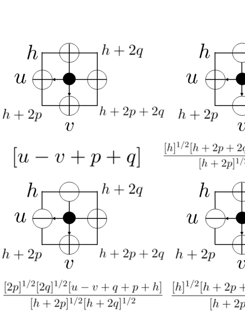
Figure 1: The matrix elements of the elliptic Felderhof model (1.11). The states $|0\rangle$, $\langle 0|$ are represented as $\oplus$, while the states $|1\rangle$, $\langle 1|$ are represented as $\ominus$. This kind of graphical representation for the case of trigonometric vertex models can be found in Bump-Brubaker-Friedberg [37] and Bump-McNamara-Nakasuji [55] for example.

We denote the orthonormal basis of $W_{a}$ and its dual as $\{|0\rangle_{a},|1\rangle_{a}\}$ and $\{{}_{a}\langle 0|,{}_{a}\langle 1|\}$, and the matrix elements of the dynamical $R$-matrix as ${}_{a}\langle\gamma|{}_{b}\langle\delta|R_{ab}(u,v|p,q|h)|\alpha\rangle_{a}|\beta\rangle_{b}=[R(u,v|p,q|h)]_{\alpha\beta}^{\gamma\delta}$. The matrix elements of the dynamical $R$-matrix are explicitly given as

$${}_{a}\langle 0|{}_{b}\langle 0|R_{ab}(u.v|p,q|h)|0\rangle_{a}|0\rangle_{b} =[u-v+p+q],$$ (1.12)

$${}_{a}\langle 0|{}_{b}\langle 1|R_{ab}(u,v|p,q|h)|0\rangle_{a}|1\rangle_{b} =\frac{[h]^{1/2}[h+2p+2q]^{1/2}[u-v+q-p]}{[h+2p]^{1/2}[h+2q]^{1/2}},$$ (1.13)

$${}_{a}\langle 0|{}_{b}\langle 1|R_{ab}(u,v|p,q|h)|1\rangle_{a}|0\rangle_{b} =\frac{[2p]^{1/2}[2q]^{1/2}[-u+v+q+p+h]}{[h+2p]^{1/2}[h+2q]^{1/2}},$$ (1.14)

$${}_{a}\langle 1|{}_{b}\langle 0|R_{ab}(u,v|p,q|h)|0\rangle_{a}|1\rangle_{b} =\frac{[2p]^{1/2}[2q]^{1/2}[u-v+q+p+h]}{[h+2p]^{1/2}[h+2q]^{1/2}},$$ (1.15)

$${}_{a}\langle 1|{}_{b}\langle 0|R_{ab}(u,v|p,q|h)|1\rangle_{a}|0\rangle_{b} =\frac{[h]^{1/2}[h+2p+2q]^{1/2}[u-v-q+p]}{[h+2p]^{1/2}[h+2q]^{1/2}},$$ (1.16)

$${}_{a}\langle 1|{}_{b}\langle 1|R_{ab}(u,v|p,q|h)|1\rangle_{a}|1\rangle_{b} =[-u+v+p+q].$$ (1.17)

In statistical physics, $|0\rangle$ or its dual $\langle 0|$ can be regarded as a hole state, while $|1\rangle$ or its dual $\langle 1|$ can be interpretted as a particle state. We thus sometimes use the terms hole states and particle states to describe states constructed from $|0\rangle$, $\langle 0|$, $|1\rangle$ and $\langle 1|$ since they are convenient for the description of the states.

For later convenience, we also define the following Pauli spin operators $\sigma^{+}$ and $\sigma^{-}$ as operators acting on the (dual) orthonomal basis as

$$\sigma^{+}|1\rangle=|0\rangle,\ \sigma^{+}|0\rangle=0,\ \langle 0|\sigma^{+}=\langle 1|,\ \langle 1|\sigma^{+}=0,$$ (1.18)

$$\sigma^{-}|0\rangle=|1\rangle,\ \sigma^{-}|1\rangle=0,\ \langle 1|\sigma^{-}=\langle 0|,\ \langle 0|\sigma^{-}=0.$$ (1.19)

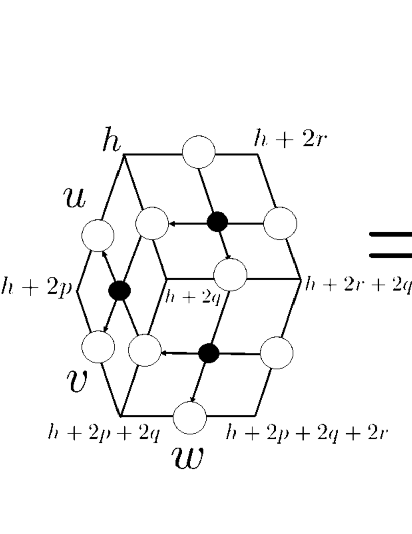
Figure 2: The dynamical Yang-Baxter relation (1.20). The left and right figure represents $R_{ab}(u,v|p,q|h)R_{ac}(u,w|p,r|h+2q)R_{bc}(v,w|q,r|h)$ and $R_{bc}(v,w|q,r|h+2p)R_{ac}(u,w|p,r|h)R_{ab}(u,v|p,q|h+2r)$, respectively.

The dynamical $R$-matrix (1.11) satisfies the dynamical Yang-Baxter (face-type Yang-Baxter, star-triangle) relation (Figure 2)

$$R_{ab}(u,v|p,q|h)R_{ac}(u,w|p,r|h+2q)R_{bc}(v,w|q,r|h)$$

$$= R_{bc}(v,w|q,r|h+2p)R_{ac}(u,w|p,r|h)R_{ab}(u,v|p,q|h+2r),$$ (1.20)

acting on $W_{a}\otimes W_{b}\otimes W_{c}$.

To construct partition functions of integrable lattice models, we identify one of the complex two-dimensional spaces $W_{b}$ of the tensor product space $W_{a}\otimes W_{b}$ with the quantum space. Let us denote the quantum space by $\mathcal{F}_{j}$, and define the $L$-operator $L_{aj}(u,v|p,q|h)$ acting on $W_{a}\otimes\mathcal{F}_{j}$ as

$$L_{aj}(u,v|p,q|h)=R_{aj}(u,v|p,q|h).$$ (1.21)

The next step is to define the monodromy matrix from the $L$-operators. For convenience, one denotes the sum of complex numbers $q_{1},q_{2},\dots,q_{j}$ as $\overline{q_{j}}$

$$\overline{q_{j}}:=\sum_{k=1}^{j}q_{k}.$$ (1.22)

The monodromy matrix $T_{a}(u|v_{1},\dots,v_{M}|p|q_{1},\dots,q_{M}|h)$ is the product of $L$-operators

$$T_{a}(u|v_{1},\dots,v_{M}|p|q_{1},\dots,q_{M}|h)$$

$$= L_{a1}(u,v_{1}|p,q_{1}|h)L_{a2}(u,v_{2}|p,q_{2}|h+2\overline{q_{1}})\cdots L_{aM}(u,v_{M}|p,q_{M}|h+2\overline{q_{M-1}}),$$ (1.23)

acting on $W_{a}\otimes\mathcal{F}_{1}\otimes\cdots\otimes\mathcal{F}_{M}$.

The $B$-operator and the $C$-operator are matrix elements of the monodromy matrix (1.23) with respect to the auxiliary space $W_{a}$

$$B(u|v_{1},\dots,v_{M}|p|q_{1},\dots,q_{M}|h) ={}_{a}\langle 0|T_{a}(u|v_{1},\dots,v_{M}|p|q_{1},\dots,q_{M}|h)|1\rangle_{a},$$ (1.24)

$$C(u|v_{1},\dots,v_{M}|p|q_{1},\dots,q_{M}|h) ={}_{a}\langle 1|T_{a}(u|v_{1},\dots,v_{M}|p|q_{1},\dots,q_{M}|h)|0\rangle_{a},$$ (1.25)

which acts on $\mathcal{F}_{1}\otimes\cdots\otimes\mathcal{F}_{M}$ and it dual $\mathcal{F}_{1}^{*}\otimes\cdots\otimes\mathcal{F}_{M}^{*}$ (Figure 3).

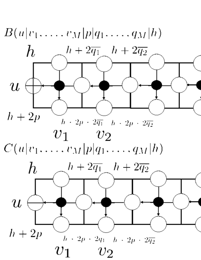
Figure 3: The $B$-operator $B(u|v_{1},\dots,v_{M}|p|q_{1},\dots,q_{M}|h)$ (1.24) (top) and the $C$-operator $C(u|v_{1},\dots,v_{M}|p|q_{1},\dots,q_{M}|h)$ (1.25) (bottom).

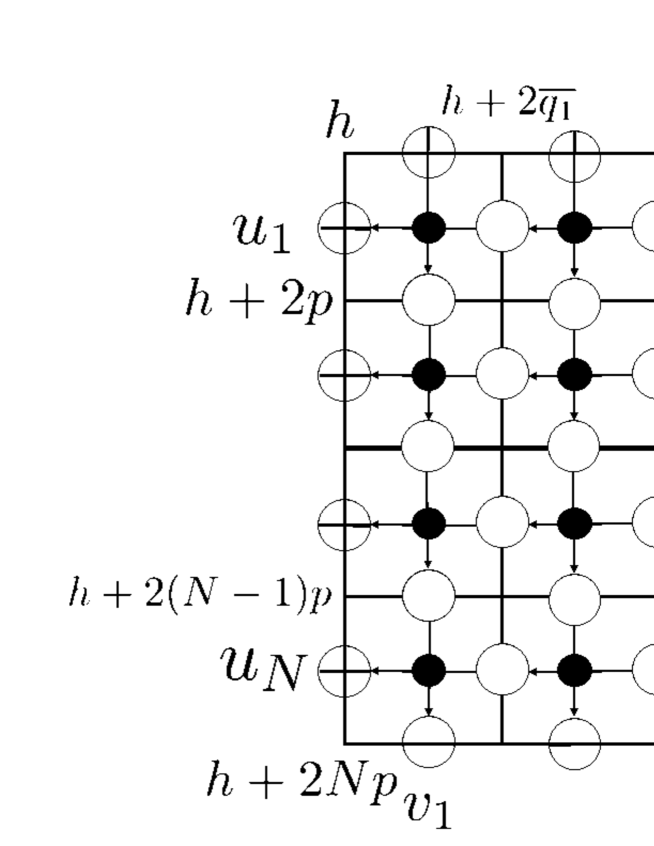
Figure 4: The domain wall boundary partition functions $Z_{N}(u_{1},\dots,u_{N}|v_{1},\dots,v_{N}|h)$ (1.26).

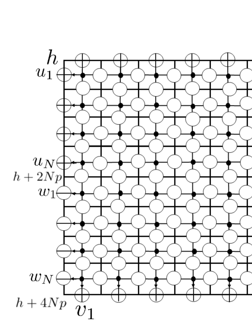
Figure 5: The scalar products $Q_{M,N}(u_{1},\dots,u_{N}|w_{1},\dots,w_{N}|v_{1},\dots,v_{M}|h)$ (2.1).

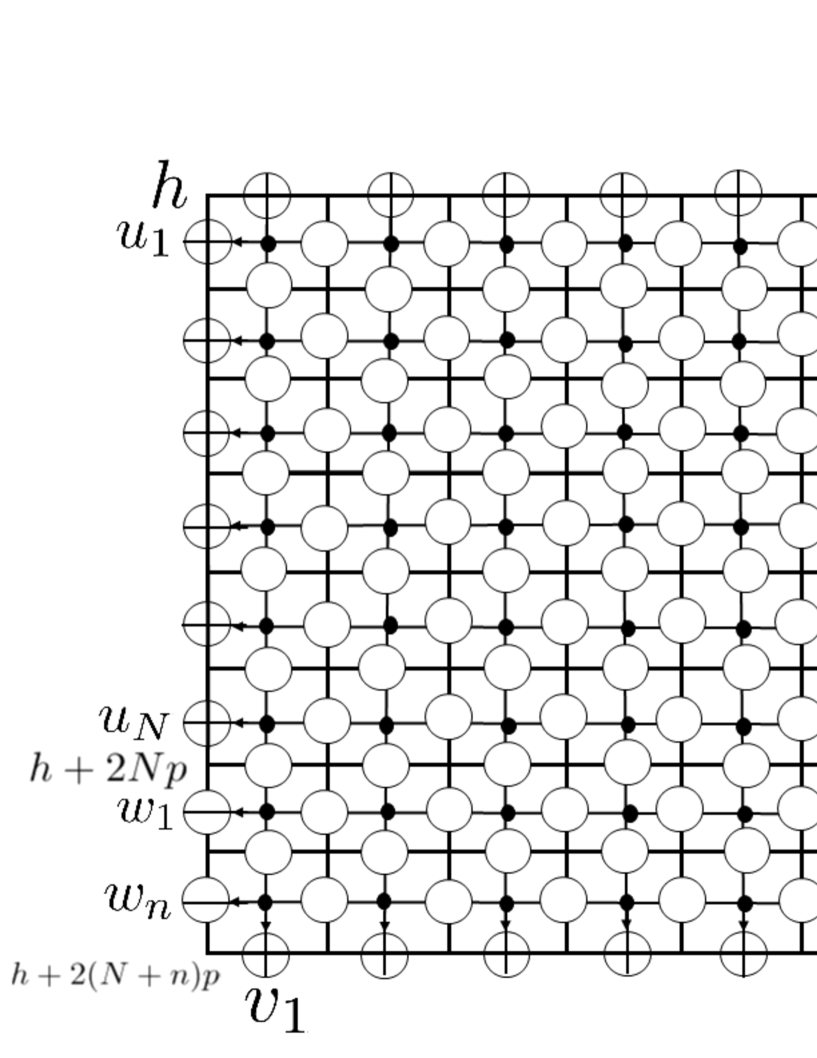
Figure 6: The intermediate scalar products $Q_{M,N,n}(u_{1},\dots,u_{N}|w_{1},\dots,w_{n}|v_{1},\dots,v_{M}|h)$ (2.1). One notes that the dynamical $R$-matrices in the right part of the bottom row are already frozen due to the ice-rule of the dynamical $R$-matrix.

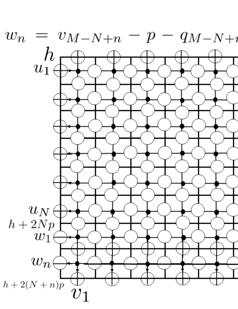
Figure 7: The intermediate scalar products $Q_{M,N,n}(u_{1},\dots,u_{N}|w_{1},\dots,w_{n}|v_{1},\dots,v_{M}|h)$ (2.1) evaluated at $w_{n}=v_{M-N+n}-p-q_{M-N+n}$, which gives (2.6) since the dynamical $R$-matrices at the bottom row are frozen and the remaining part is $Q_{M,N,n-1}(u_{1},\dots,u_{N}|w_{1},\dots,w_{n-1}|v_{1},\dots,v_{M}|h)$.

The following domain wall boundary partition functions (Figure 4) is one of the most well-investigated classes of partition functions [41]

$$Z_{N}(u_{1},\dots,u_{N}|v_{1},\dots,v_{N}|h)={}_{N}\langle\overline{\Omega}|B(u_{N}|v_{1},\dots,v_{M}|p|q_{1},\dots,q_{M}|h+2(N-1)p)$$

$$\times\cdots\times B(u_{2}|v_{1},\dots,v_{M}|p|q_{1},\dots,q_{M}|h+2p)B(u_{1}|v_{1},\dots,v_{M}|p|q_{1},\dots,q_{M}|h)|\Omega\rangle_{N}.$$ (1.26)

Here, $|\Omega\rangle_{N}:=|0\rangle_{1}\otimes\cdots\otimes|0\rangle_{N}\in\mathcal{F}_{1}\otimes\cdots\otimes\mathcal{F}_{N}$ and ${}_{N}\langle\overline{\Omega}|:={}_{1}\langle 1|\otimes\cdots\otimes{}_{N}\langle 1|\in\mathcal{F}_{1}^{*}\otimes\cdots\otimes\mathcal{F}_{N}^{*}$ are the vacuum state and the dual particle-occupied state in the tensor product of quantum spaces.

In the paper in which the elliptic Felderhof model was introduced, Foda-Wheeler-Zuparic showed the following factorized expression for the domain wall boundary partition functions [30, 63, 64].

Theorem 1.2.

(Foda-Wheeler-Zuparic [30]) The domain wall boundary partition functions of the elliptic Felderhof model $Z_{N}(u_{1},\dots,u_{N}|v_{1},\dots,v_{N}|h)$ has the following factorized form

$$Z_{N}(u_{1},\dots,u_{N}|v_{1},\dots,v_{N}|h)= \frac{[h+\sum_{j=1}^{N}v_{j}-\sum_{j=1}^{N}u_{j}+Np+\sum_{j=1}^{N}q_{j}]}{[h+2\sum_{j=1}^{N}q_{j}]^{1/2}[h+2Np]^{1/2}}$$

$$\times\prod_{j=1}^{N}[2p]^{1/2}[2q_{j}]^{1/2}\prod_{1\leq j<k\leq N}[u_{j}-u_{k}+2p][v_{k}-v_{j}+q_{j}+q_{k}].$$ (1.27)

We use (1.27) for the analysis on the scalar products of the elliptic Felderhof model in the next section.

2 Scalar Products

In this section, we introduce the scalar products of the Foda-Wheeler-Zuparic model, and prove the determinant formula. The scalar products are defined as the following partition functions (Figure 5)

$$Q_{M,N}(u_{1},\dots,u_{N}|w_{1},\dots,w_{N}|v_{1},\dots,v_{M}|h)$$

$$= {}_{M}\langle\Omega|C(w_{N}|v_{1},\dots,v_{M}|p|q_{1},\dots,q_{M}|h+2(2N-1)p)$$

$$\times\cdots\times C(w_{1}|v_{1},\dots,v_{M}|p|q_{1},\dots,q_{M}|h+2Np)$$

$$\times B(u_{N}|v_{1},\dots,v_{M}|p|q_{1},\dots,q_{M}|h+2(N-1)p)$$

$$\times\cdots\times B(u_{1}|v_{1},\dots,v_{M}|p|q_{1},\dots,q_{M}|h)|\Omega\rangle_{M},$$ (2.1)

where $|\Omega\rangle_{M}:=|0\rangle_{1}\otimes\cdots\otimes|0\rangle_{M}\in\mathcal{F}_{1}\otimes\cdots\otimes\mathcal{F}_{M}$ and ${}_{M}\langle\Omega|:={}_{1}\langle 0|\otimes\cdots\otimes{}_{M}\langle 0|\in\mathcal{F}_{1}^{*}\otimes\cdots\otimes\mathcal{F}_{M}^{*}$ are the vacuum state and the dual vacuum state in the tensor product of quantum spaces.

The main result of this paper is the following determinant formula for the scalar products of the elliptic Felderhof model.

Theorem 2.1.

We have the following determinant formula for the scalar products of the elliptic Felderhof model

$$Q_{M,N}(u_{1},\dots,u_{N}|w_{1},\dots,w_{N}|v_{1},\dots,v_{M}|h)$$

$$= [2p]^{N}\frac{[h+2Np]^{1/2}[h+2Np+2\overline{q_{M}}]^{1/2}}{[h+4Np]^{1/2}[h+2\overline{q_{M}}]^{1/2}}\prod_{1\leq j<k\leq N}\frac{[u_{j}-u_{k}+2p][w_{j}-w_{k}-2p]}{[u_{j}-u_{k}][w_{j}-w_{k}]}$$

$$\times\mathrm{det}_{N}\Bigg{(}\frac{\frac{[w_{j}+h+2Np-u_{k}]}{[h+2Np]}a(w_{j})d(u_{k})-\frac{[w_{j}+h+2Np-u_{k}+2\overline{q_{M}}]}{[h+2Np+2\overline{q_{M}}]}a(u_{k})d(w_{j})}{[u_{k}-w_{j}]}\Bigg{)},$$ (2.2)

where $\overline{q_{j}}=\sum_{k=1}^{j}q_{k}$, and $a(u)$ and $d(u)$ are given by

$$a(u)=\prod_{\ell=1}^{M}[u-v_{\ell}+p+q_{\ell}],\ \ \ d(u)=\prod_{\ell=1}^{M}[u-v_{\ell}+p-q_{\ell}].$$ (2.3)

We apply Wheeler’s method [79] which extends the Izergin-Korpein technique [42, 41] from the domain wall boundary partition functions to the scalar products. To this end, we introduce the following intermediate scalar products [79] which is an intermediate object between the scalar products and the domain wall boundary partition functions (Figure 6)

$$Q_{M,N,n}(u_{1},\dots,u_{N}|w_{1},\dots,w_{n}|v_{1},\dots,v_{M}|h)$$

$$= \langle 0^{M-N+n}1^{N-n}|C(w_{n}|v_{1},\dots,v_{M}|p|q_{1},\dots,q_{M}|h+2(N+n-1)p)$$

$$\times\cdots\times C(w_{1}|v_{1},\dots,v_{M}|p|q_{1},\dots,q_{M}|h+2Np)$$

$$\times B(u_{N}|v_{1},\dots,v_{M}|p|q_{1},\dots,q_{M}|h+2(N-1)p)$$

$$\times\cdots\times B(u_{1}|v_{1},\dots,v_{M}|p|q_{1},\dots,q_{M}|h)|\Omega\rangle_{M},$$ (2.4)

where

$$\langle 0^{M-N+n}1^{N-n}|={}_{1}\langle 0|\otimes\cdots\otimes{}_{M-N+n}\langle 0|\otimes{}_{M-N+n+1}\langle 1|\otimes\cdots\otimes{}_{M}\langle 1|.$$ (2.5)

The special case $n=N$ of the intermediate scalar products corresponds to the scalar products $Q_{M,N}(u_{1},\dots,u_{N}|w_{1},\dots,w_{N}|v_{1},\dots,v_{M}|h)$, while the case $n=0$ is essentially the domain wall boundary partition functions.

The first thing to do is to list the properties of the intermediate scalar products which uniquely characterize it, which is given below.

Proposition 2.2.

The intermediate scalar products of the elliptic Felderhof model
$Q_{M,N,n}(u_{1},\dots,u_{N}|w_{1},\dots,w_{n}|v_{1},\dots,v_{M}|h)$ satisfies the following properties.

(1) $\displaystyle\prod_{j=M-N+n+1}^{M}[w_{n}-v_{j}+q_{j}-p]^{-1}Q_{M,N,n}(u_{1},\dots,u_{N}|w_{1},\dots,w_{n}|v_{1},\dots,v_{M}|h)$ is an elliptic polynomial of $w_{n}$ in $\Theta_{M-N+n}(\chi)$.

(2) The intermediate scalar products $Q_{M,N,n}(u_{1},\dots,u_{N}|w_{1},\dots,w_{n}|v_{1},\dots,v_{M}|h)$ is invariant under the simultaneous exchange of $v_{j}$, $q_{j}$ and $v_{k}$, $q_{k}$ for $1\leq j<k\leq M-N+n$.

(3) The following recursive relations between the intermediate scalar products hold:

$$Q_{M,N,n}(u_{1},\dots,u_{N}|w_{1},\dots,w_{n}|v_{1},\dots,v_{M}|h)|_{w_{n}=v_{M-N+n}-p-q_{M-N+n}}=[2p]^{1/2}[2q_{M-N+n}]^{1/2}$$

$$\times\frac{[h+2(N+n-1)p]^{1/2}[h+2(N+n-1)p+2\overline{q_{M-N+n-1}}]^{1/2}[h+2(N+n)p+2\overline{q_{M}}]^{1/2}}{[h+2(N+n)p]^{1/2}[h+2(N+n)p+2\overline{q_{M-N+n}}]^{1/2}[h+2(N+n-1)p+2\overline{q_{M}}]^{1/2}}$$

$$\times\prod_{j=1}^{M-N+n-1}[v_{M-N+n}-q_{M-N+n}-v_{j}-q_{j}]\prod_{j=M-N+n+1}^{M}[v_{M-N+n}-q_{M-N+n}-v_{j}+q_{j}-2p]$$

$$\times Q_{M,N,n-1}(u_{1},\dots,u_{N}|w_{1},\dots,w_{n-1}|v_{1},\dots,v_{M}|h).$$ (2.6)

(4) The following evaluation holds for the case $n=0$

$$Q_{M,N,0}(u_{1},\dots,u_{N}||v_{1},\dots,v_{M}|h)=\frac{[h+2Np+2\overline{q_{M}}]}{[h+2\overline{q_{M}}]^{1/2}[h+2\overline{q_{M-N}}+2Np]^{1/2}}$$

$$\times\prod_{1\leq j<k\leq N}\frac{[u_{j}-u_{k}+2p]}{[u_{j}-u_{k}]}\prod_{M-N+1\leq j<k\leq M}\frac{[v_{k}-v_{j}+q_{j}+q_{k}]}{[v_{k}-v_{j}+q_{j}-q_{k}]}\prod_{j=1}^{N}\prod_{k=1}^{M}[u_{j}-v_{k}+p+q_{k}]$$

$$\times\prod_{j=1}^{N}[2p]^{1/2}\prod_{j=M-N+1}^{M}[2q_{j}]^{1/2}\mathrm{det}_{N}\Bigg{(}\frac{[h+(2N-1)p+2\overline{q_{M}}-q_{M-N+k}+v_{M-N+k}-u_{j}]}{[h+2Np+2\overline{q_{M}}][u_{j}+p-v_{M-N+k}+q_{M-N+k}]}\Bigg{)}.$$ (2.7)

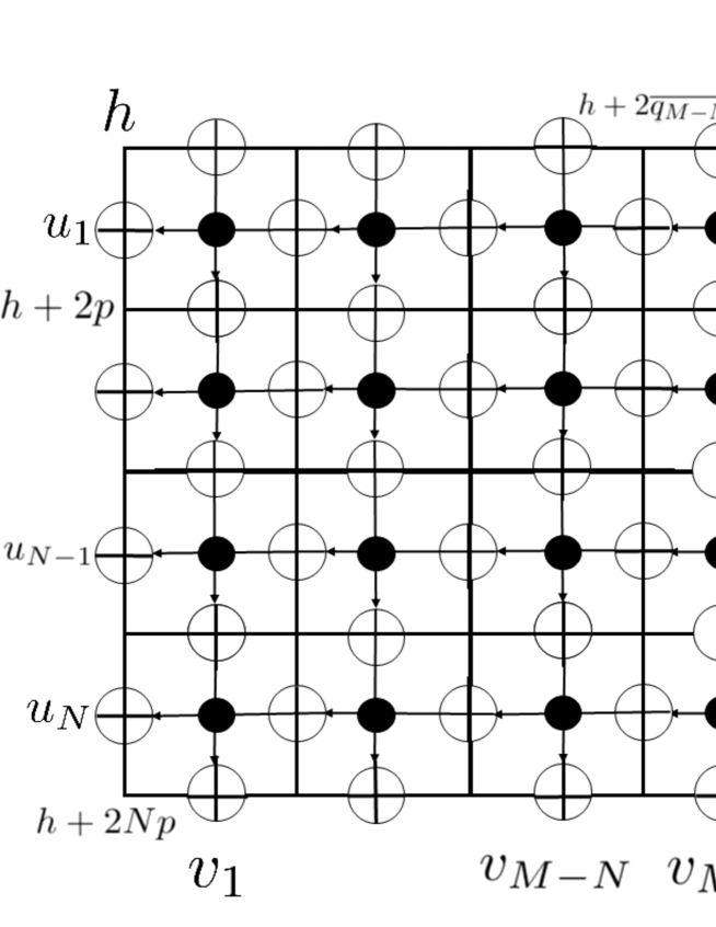
Figure 8: The intermediate scalar products $Q_{M,N,0}(u_{1},\dots,u_{N}||v_{1},\dots,v_{M}|h)$. One can see that the inner states of the left part of the lattice models are frozen which make contribution $\prod_{j=1}^{N}\prod_{k=1}^{M-N}[u_{j}-v_{k}+p+q_{k}]$ to the intermediate scalar products, and the right unfrozen part are the domain wall boundary partition functions $Z_{N}(u_{1},\dots,u_{N}|v_{M-N+1},\dots,v_{M}|h+2\overline{q_{M-N}})$.

Proof.

Properties (1), (2) and (3) can be shown by using standard arguments.

Property (1) can be shown as follows. We insert the completeness relation into the intermediate scalar products

$$Q_{M,N,n}(u_{1},\dots,u_{N}|w_{1},\dots,w_{n}|v_{1},\dots,v_{M}|h)$$

$$= \langle 0^{M-N+n}1^{N-n}|C(w_{n}|v_{1},\dots,v_{M}|p|q_{1},\dots,q_{M}|h+2(N+n-1)p)$$

$$\times\cdots\times C(w_{1}|v_{1},\dots,v_{M}|p|q_{1},\dots,q_{M}|h+2Np)$$

$$\times B(u_{N}|v_{1},\dots,v_{M}|p|q_{1},\dots,q_{M}|h+2(N-1)p)$$

$$\times\cdots\times B(u_{1}|v_{1},\dots,v_{M}|p|q_{1},\dots,q_{M}|h)|\Omega\rangle_{M}$$

$$= \sum_{k=1}^{M-N+n}\langle 0^{M-N+n}1^{N-n}|C(w_{n}|v_{1},\dots,v_{M}|p|q_{1},\dots,q_{M}|h+2(N+n-1)p)|0^{k-1}10^{M-N+n-k}1^{N-n}\rangle$$

$$\times\langle 0^{k-1}10^{M-N+n-k}1^{N-n}|C(w_{n-1}|v_{1},\dots,v_{M}|p|q_{1},\dots,q_{M}|h+2(N+n-2)p)\times\cdots\times$$

$$\times C(w_{1}|v_{1},\dots,v_{M}|p|q_{1},\dots,q_{M}|h+2Np)B(u_{N}|v_{1},\dots,v_{M}|p|q_{1},\dots,q_{M}|h+2(N-1)p)\times$$

$$\times\cdots\times B(u_{1}|v_{1},\dots,v_{M}|p|q_{1},\dots,q_{M}|h)|\Omega\rangle_{M}.$$ (2.8)

We calculate the matrix elements of $C(w_{n}|v_{1},\dots,v_{M}|p|q_{1},\dots,q_{M}|h+2(N+n-1)p)$ based on its definition to get

$$\langle 0^{M-N+n}1^{N-n}|C(w_{n}|v_{1},\dots,v_{M}|p|q_{1},\dots,q_{M}|h+2(N+n-1)p)|0^{k-1}10^{M-N+n-k}1^{N-n}\rangle$$

$$= \prod_{j=1}^{k-1}\frac{[h+2(N+n-1)p+2\overline{q_{j-1}}]^{1/2}[h+2(N+n)p+2\overline{q_{j}}]^{1/2}[w_{n}-v_{j}-q_{j}+p]}{[h+2(N+n)p+2\overline{q_{j-1}}]^{1/2}[h+2(N+n-1)p+2\overline{q_{j}}]^{1/2}}$$

$$\times\frac{[2p]^{1/2}[2q_{k}]^{1/2}[w_{n}-v_{k}+q_{k}+p+h+2(N+n-1)p+2\overline{q_{k-1}}]}{[h+2(N+n)p+2\overline{q_{k-1}}]^{1/2}[h+2(N+n-1)p+2\overline{q_{k}}]^{1/2}}\prod_{j=k+1}^{M-N+n}[w_{n}-v_{j}+p+q_{j}]$$

$$\times\prod_{j=M-N+n+1}^{M}\frac{[h+2(N+n-1)p+2\overline{q_{j-1}}]^{1/2}[h+2(N+n)p+2\overline{q_{j}}]^{1/2}[w_{n}-v_{j}+q_{j}-p]}{[h+2(N+n)p+2\overline{q_{j-1}}]^{1/2}[h+2(N+n-1)p+2\overline{q_{j}}]^{1/2}}.$$ (2.9)

One can see from (2.9) that $Q_{M,N,n}(u_{1},\dots,u_{N}|w_{1},\dots,w_{n}|v_{1},\dots,v_{M}|h)$ has $\displaystyle\prod_{j=M-N+n+1}^{M}[w_{n}-v_{j}+q_{j}-p]$ as an overall factor (one can also show this by the graphical representation of the intermediate scalar products in Figure 6, in which one can show that the dynamical $R$-matrices of the right part of the bottom row are already frozen due to the ice-rule of the dynamical $R$-matrix, and the matrix elements of the $R$-matrices of the frozen parts contain the factor $\displaystyle\prod_{j=M-N+n+1}^{M}[w_{n}-v_{j}+q_{j}-p]$). Let us denote the intermediate scalar products divided by this factor as $\widetilde{Q}_{M,N,n}(u_{1},\dots,u_{N}|w_{1},\dots,w_{n}|v_{1},\dots,v_{M}|h)$:

$$\widetilde{Q}_{M,N,n}(u_{1},\dots,u_{N}|w_{1},\dots,w_{n}|v_{1},\dots,v_{M}|h)$$

$$= \prod_{j=M-N+n+1}^{M}[w_{n}-v_{j}+q_{j}-p]^{-1}Q_{M,N,n}(u_{1},\dots,u_{N}|w_{1},\dots,w_{n}|v_{1},\dots,v_{M}|h).$$ (2.10)

By calculating the quasi-periodicities of $\langle 0^{M-N+n}1^{N-n}|C(w_{n}|v_{1},\dots,v_{M}|p|q_{1},\dots,q_{M}|h+2(N+n-1)p)|0^{k-1}10^{M-N+n-k}1^{N-n}\rangle$ with respect to $w_{n}$, one finds those of the elliptic functions $\widetilde{Q}_{M,N,n}(u_{1},\dots,u_{N}|w_{1},\dots,w_{n}|v_{1},\dots,v_{M}|h)$ are given by

$$\widetilde{Q}_{M,N,n}(u_{1},\dots,u_{N}|w_{1},\dots,w_{n}+1|v_{1},\dots,v_{M}|h)$$

$$= (-1)^{M-N+n}\widetilde{Q}_{M,N,n}(u_{1},\dots,u_{N}|w_{1},\dots,w_{n}|v_{1},\dots,v_{M}|h),$$ (2.11)

$$\widetilde{Q}_{M,N,n}(u_{1},\dots,u_{N}|w_{1},\dots,w_{n}-i\mathrm{log}({\bf q})/\pi|v_{1},\dots,v_{M}|h)$$

$$= (-{\bf q}^{-1})^{M-N+n}\mathrm{exp}\Bigg{(}-2\pi i\Bigg{(}(M-N+n)w_{n}+h+(M+N+3n-2)p$$

$$-\sum_{j=1}^{M-N+n}v_{j}+\sum_{j=1}^{M-N+n}q_{j}\Bigg{)}\Bigg{)}\widetilde{Q}_{M,N,n}(u_{1},\dots,u_{N}|w_{1},\dots,w_{n}|v_{1},\dots,v_{M}|h),$$ (2.12)

which shows that $\widetilde{Q}_{M,N,n}(u_{1},\dots,u_{N}|w_{1},\dots,w_{n}|v_{1},\dots,v_{M}|h)$ is an elliptic polynomial of $w_{n}$ in $\Theta_{M-N+n}(\chi)$ of periods $1$ and $\tau=-i\mathrm{log}({\bf q})/\pi$ with the characters $\chi(1)=(-1)^{M-N+n}$ and
$\displaystyle\chi(\tau)=\mathrm{exp}\Bigg{(}-2\pi i\Bigg{(}h+(M+N+3n-2)p-\sum_{j=1}^{M-N+n}v_{j}+\sum_{j=1}^{M-N+n}q_{j}\Bigg{)}\Bigg{)}$. This shows Property (1).

Property (2) can be shown as a consequence of the the commutation relation between the vertical monodromy matrices, which is a standard procedure using the dynamical Yang-Baxter relation, thus we omit the details.

Property (3) can be shown by substituting $w_{n}=v_{M-N+n}-p-q_{M-N+n}$ into (2.8), after which only one of the summands $k=M-N+n$ survives. Equivalently, this property can also be shown by the graphical description of the intermediate scalar products (Figure 7).

Let us show Property (4). From its graphical description (Figure 8), one easily finds that for the case $n=0$, the intermediate scalar products $Q_{M,N,0}(u_{1},\dots,u_{N}||v_{1},\dots,v_{M}|h)$ is just a concatenation of frozen parts and the domain wall boundary partition functions

$$Q_{M,N,0}(u_{1},\dots,u_{N}||v_{1},\dots,v_{M}|h)$$

$$= \prod_{j=1}^{N}\prod_{k=1}^{M-N}[u_{j}-v_{k}+p+q_{k}]Z_{N}(u_{1},\dots,u_{N}|v_{M-N+1},\dots,v_{M}|h+2\overline{q_{M-N}}).$$ (2.13)

We insert the factorization formula for the domain wall boundary partition functions by Foda-Wheeler-Zuparic ((1.27) in Theorem 1.2) into the right hand side of (2.13) to get

$$Q_{M,N,0}(u_{1},\dots,u_{N}||v_{1},\dots,v_{M}|h)$$

$$= \prod_{j=1}^{N}\prod_{k=1}^{M-N}[u_{j}-v_{k}+p+q_{k}]$$

$$\times\frac{\displaystyle\Bigg{[}h+2\overline{q_{M-N}}+\sum_{j=M-N+1}^{M}v_{j}-\sum_{j=1}^{N}u_{j}+Np+\sum_{j=M-N+1}^{M}q_{j}\Bigg{]}}{[h+2\overline{q_{M}}]^{1/2}[h+2\overline{q_{M-N}}+2Np]^{1/2}}$$

$$\times\prod_{j=1}^{N}[2p]^{1/2}\prod_{j=M-N+1}^{M}[2q_{j}]^{1/2}\prod_{1\leq j<k\leq N}[u_{j}-u_{k}+2p]\prod_{M-N+1\leq j<k\leq M}[v_{k}-v_{j}+q_{j}+q_{k}].$$ (2.14)

(2.14) is already an explicit form corresponding to the initial condition of the Izergin-Korepin recursion process between the intermediate scalar products, and is a very compact expression since it is a factorized form. However, we further rewrite it in a determinant form. Going back to a complicated expression is because in the next proposition, we present the explicit determinant form of the intermediate scalar products, and we have to check that it satisfies the case $n=0$, which is immediate to see if one rewrites in the determinant form (2.7).

How to rewrite (2.14) in the determinant form goes as follows. We set $\lambda=-h-2Np-2\overline{q_{M}}$, $z_{j}=u_{j}+p$, $w_{k}=v_{M-N+k}-q_{M-N+k}$ into the Frobenius determinant formula

$$\mathrm{det}_{N}\Bigg{(}\frac{[\lambda+z_{j}-w_{k}]}{[\lambda][z_{j}-w_{k}]}\Bigg{)}=\frac{\displaystyle[\lambda+\sum_{j=1}^{N}(z_{j}-w_{j})]\prod_{1\leq j<k\leq N}[z_{j}-z_{k}][w_{k}-w_{j}]}{\displaystyle[\lambda]\prod_{1\leq j,k\leq N}[z_{j}-w_{k}]},$$ (2.15)

to get the following identity

$$\Bigg{[}h+2\overline{q_{M-N}}+\sum_{j=M-N+1}^{M}v_{j}-\sum_{j=1}^{N}u_{j}+Np+\sum_{j=M-N+1}^{M}q_{j}\Bigg{]}$$

$$= \frac{\displaystyle[h+2Np+2\overline{q_{M}}]\prod_{j=1}^{N}\prod_{k=M-N+1}^{M}[u_{j}+p-v_{k}+q_{k}]}{\displaystyle\prod_{1\leq j<k\leq N}[u_{j}-u_{k}]\prod_{M-N+1\leq j<k\leq M}[v_{k}-v_{j}-q_{k}+q_{j}]}$$

$$\times\mathrm{det}_{N}\Bigg{(}\frac{[h+(2N-1)p+2\overline{q_{M}}-q_{M-N+k}+v_{M-N+k}-u_{j}]}{[h+2Np+2\overline{q_{M}}][u_{j}+p-v_{M-N+k}+q_{M-N+k}]}\Bigg{)}.$$ (2.16)

Substituting (2.16) into the right hand side of (2.14), we get

$$Q_{M,N,0}(u_{1},\dots,u_{N}||v_{1},\dots,v_{M}|h)$$

$$= \frac{1}{[h+2\overline{q_{M}}]^{1/2}[h+2\overline{q_{M-N}}+2Np]^{1/2}}\prod_{j=1}^{N}\prod_{k=1}^{M-N}[u_{j}-v_{k}+p+q_{k}]$$

$$\times\frac{\displaystyle[h+2Np+2\overline{q_{M}}]\prod_{j=1}^{N}\prod_{k=M-N+1}^{M}[u_{j}+p-v_{k}+q_{k}]}{\displaystyle\prod_{1\leq j<k\leq N}[u_{j}-u_{k}]\prod_{M-N+1\leq j<k\leq M}[v_{k}-v_{j}-q_{k}+q_{j}]}$$

$$\times\mathrm{det}_{N}\Bigg{(}\frac{[h+(2N-1)p+2\overline{q_{M}}-q_{M-N+k}+v_{M-N+k}-u_{j}]}{[h+2Np+2\overline{q_{M}}][u_{j}+p-v_{M-N+k}+q_{M-N+k}]}\Bigg{)}$$

$$\times\prod_{j=1}^{N}[2p]^{1/2}\prod_{j=M-N+1}^{M}[2q_{j}]^{1/2}\prod_{1\leq j<k\leq N}[u_{j}-u_{k}+2p]\prod_{M-N+1\leq j<k\leq M}[v_{k}-v_{j}+q_{j}+q_{k}]$$

$$= \frac{[h+2Np+2\overline{q_{M}}]}{[h+2\overline{q_{M}}]^{1/2}[h+2\overline{q_{M-N}}+2Np]^{1/2}}$$

$$\times\prod_{1\leq j<k\leq N}\frac{[u_{j}-u_{k}+2p]}{[u_{j}-u_{k}]}\prod_{M-N+1\leq j<k\leq M}\frac{[v_{k}-v_{j}+q_{j}+q_{k}]}{[v_{k}-v_{j}+q_{j}-q_{k}]}\prod_{j=1}^{N}\prod_{k=1}^{M}[u_{j}-v_{k}+p+q_{k}]$$

$$\times\prod_{j=1}^{N}[2p]^{1/2}\prod_{j=M-N+1}^{M}[2q_{j}]^{1/2}\mathrm{det}_{N}\Bigg{(}\frac{[h+(2N-1)p+2\overline{q_{M}}-q_{M-N+k}+v_{M-N+k}-u_{j}]}{[h+2Np+2\overline{q_{M}}][u_{j}+p-v_{M-N+k}+q_{M-N+k}]}\Bigg{)},$$ (2.17)

and Property (4) is proved.

∎

The next thing to do is to find the explicit forms of the intermediate scalar products satisfying all the properties in Proposition 2.2. One can show the following determinant representation.

Theorem 2.3.

The intermediate scalar products $Q_{M,N,n}(u_{1},\dots,u_{N}|w_{1},\dots,w_{n}|v_{1},\dots,v_{M}|h)$ have the following determinant form:

$$Q_{M,N,n}(u_{1},\dots,u_{N}|w_{1},\dots,w_{n}|v_{1},\dots,v_{M}|h)$$

$$= D_{M,N,n}\prod_{1\leq j<k\leq N}\frac{[u_{j}-u_{k}+2p]}{[u_{j}-u_{k}]}\prod_{M-N+n+1\leq j<k\leq M}\frac{[v_{k}-v_{j}+q_{j}+q_{k}]}{[v_{k}-v_{j}+q_{j}-q_{k}]}$$

$$\times\prod_{1\leq j<k\leq n}\frac{[w_{j}-w_{k}-2p]}{[w_{j}-w_{k}]}\mathrm{det}_{N}\Bigg{(}P_{M,N,n}(u_{1},\dots,u_{N}|w_{1},\dots,w_{n}|v_{1},\dots,v_{M}|h)\Bigg{)},$$ (2.18)

where $D_{M,N,n}$ is given by

$$D_{M,N,n}= [2p]^{(N+n)/2}\prod_{j=n+1}^{N}[2q_{M-N+j}]^{1/2}$$

$$\times\frac{[h+2Np]^{1/2}[h+2Np+2\overline{q_{M}}]^{1/2}[h+2(N+n)p+2\overline{q_{M}}]^{1/2}}{[h+2\overline{q_{M}}]^{1/2}[h+2(N+n)p]^{1/2}[h+2(N+n)p+2\overline{q_{M-N+n}}]^{1/2}},$$ (2.19)

and $P_{M,N,n}(u_{1},\dots,u_{N}|w_{1},\dots,w_{n}|v_{1},\dots,v_{M}|h)$ is an $N\times N$ matrix whose matrix elements are given by

$$P_{M,N,n}(u_{1},\dots,u_{N}|w_{1},\dots,w_{n}|v_{1},\dots,v_{M}|h)_{jk}$$

$$= \begin{cases}\displaystyle\prod_{\ell=M-N+n+1}^{M}\frac{\displaystyle[w_{j}-v_{\ell}-p+q_{\ell}]}{\displaystyle[w_{j}-v_{\ell}+p+q_{\ell}]}\frac{\frac{[w_{j}+h+2Np-u_{k}]}{[h+2Np]}a(w_{j})d(u_{k})-\frac{[w_{j}+h+2Np-u_{k}+2\overline{q_{M}}]}{[h+2Np+2\overline{q_{M}}]}a(u_{k})d(w_{j})}{[u_{k}-w_{j}]},\\ \text{ ($1\leq j\leq n$)}\\ \displaystyle\frac{[h+(2N-1)p+2\overline{q_{M}}-q_{M-N+j}+v_{M-N+j}-u_{k}]}{[h+2Np+2\overline{q_{M}}]}\prod_{\begin{subarray}{c}\ell=1\\ \ell\neq M-N+j\end{subarray}}^{M}[u_{k}-v_{\ell}+p+q_{\ell}],\\ \text{ ($n+1\leq j\leq N$)}\end{cases}.$$ (2.20)

Proof.

One can check directly that the right hand side of (2.18) satisfies Properties (1), (2), (3) and (4) in Proposition 2.2. We give some comments. Let us denote the right hand side of (2.18) as $R_{M,N,n}(u_{1},\dots,u_{N}|w_{1},\dots,w_{n}|v_{1},\dots,v_{M}|h)$ and set

$$\widetilde{R}_{M,N,n}(u_{1},\dots,u_{N}|w_{1},\dots,w_{n}|v_{1},\dots,v_{M}|h)$$

$$= \displaystyle\prod_{j=M-N+n+1}^{M}[w_{n}-v_{j}+q_{j}-p]^{-1}R_{M,N,n}(u_{1},\dots,u_{N}|w_{1},\dots,w_{n}|v_{1},\dots,v_{M}|h).$$ (2.21)

Property (1) can be shown by calculating the quasiperiodicites of the function
$\widetilde{R}_{M,N,n}(u_{1},\dots,u_{N}|w_{1},\dots,w_{n}|v_{1},\dots,v_{M}|h)$ with respect to $w_{n}$. Expanding the determinant in the right hand side of (2.18), recalling that $a(u)$ and $d(u)$ are defined as

$$a(u)=\prod_{\ell=1}^{M}[u-v_{\ell}+p+q_{\ell}],\ \ \ d(u)=\prod_{\ell=1}^{M}[u-v_{\ell}+p-q_{\ell}],$$ (2.22)

concentrating on the factors depending on $w_{n}$, one finds

$$\widetilde{R}_{M,N,n}(u_{1},\dots,u_{N}|w_{1},\dots,w_{n}+1|v_{1},\dots,v_{M}|h)$$

$$= (-1)^{M-N+n}\widetilde{R}_{M,N,n}(u_{1},\dots,u_{N}|w_{1},\dots,w_{n}|v_{1},\dots,v_{M}|h),$$ (2.23)

$$\widetilde{R}_{M,N,n}(u_{1},\dots,u_{N}|w_{1},\dots,w_{n}-i\mathrm{log}({\bf q})/\pi|v_{1},\dots,v_{M}|h)$$

$$= (-{\bf q}^{-1})^{M-N+n}\mathrm{exp}\Bigg{(}-2\pi i\Bigg{(}(M-N+n)w_{n}+h+(M+N+3n-2)p$$

$$-\sum_{j=1}^{M-N+n}v_{j}+\sum_{j=1}^{M-N+n}q_{j}\Bigg{)}\Bigg{)}\widetilde{R}_{M,N,n}(u_{1},\dots,u_{N}|w_{1},\dots,w_{n}|v_{1},\dots,v_{M}|h),$$ (2.24)

which are exactly the same with those for $\widetilde{Q}_{M,N,n}(u_{1},\dots,u_{N}|w_{1},\dots,w_{n}+1|v_{1},\dots,v_{M}|h)$ (2.11) and (2.12).

One can also show that $\widetilde{R}_{M,N,n}(u_{1},\dots,u_{N}|w_{1},\dots,w_{n}+1|v_{1},\dots,v_{M}|h)$ has apparent singularities at $w_{n}=u_{j}$, $j=1,\dots,n$ coming from the zeroes of the denominators of the matrix elements (2.20), which cancel with the corresponding zeroes of the numerators. There are also apparent singularities at $w_{n}=w_{j}$, $j=1,\dots,n-1$ and $w_{n}=v_{\ell}-p-q_{\ell}$, $\ell=M-N+n+1,\dots,M$. Again, one finds that in these cases two rows of the matrix $P_{M,N,n}(u_{1},\dots,u_{N}|w_{1},\dots,w_{n}|v_{1},\dots,v_{M}|h)$ become proportional when taking the limits $w_{n}\to w_{j}$, $j=1,\dots,n-1$ or $w_{n}\to v_{\ell}-p-q_{\ell}$, $\ell=M-N+n+1,\dots,M$, hence there are no singularities and $\widetilde{R}_{M,N,n}(u_{1},\dots,u_{N}|w_{1},\dots,w_{n}+1|v_{1},\dots,v_{M}|h)$ is an elliptic polynomial as a function of $w_{n}$.

Property (2) can be easily checked by recalling that $\overline{q_{M}}$ and $\overline{q_{M-N+n}}$ which appear in $R_{M,N,n}(u_{1},\dots,u_{N}|w_{1},\dots,w_{n}|v_{1},\dots,v_{M}|h)$ are defined as $\displaystyle\overline{q_{M}}=\sum_{j=1}^{M}q_{j}$ and $\displaystyle\overline{q_{M-N+n}}=\sum_{j=1}^{M-N+n}q_{j}$ from which one can see that they are invariant under the exchange of $q_{j}$ and $q_{k}$ for $1\leq j<k\leq M-N+n$. Property (3) can be checked by a long and tedious but straightforward computation. We remark that expanding the determinant in the right hand side of (2.18) $\displaystyle\mathrm{det}_{N}\Bigg{(}P_{M,N,n}(u_{1},\dots,u_{N}|w_{1},\dots,w_{n}|v_{1},\dots,v_{M}|h)\Bigg{)}$ based on its definition, and rewriting the prefactor $D_{M,N,n}$ in the function $R_{M,N,n}(u_{1},\dots,u_{N}|w_{1},\dots,w_{n}|v_{1},\dots,v_{M}|h)$ as

$$D_{M,N,n}$$

$$= \frac{[h+2Np+2\overline{q_{M}}]}{[h+2\overline{q_{M}}]^{1/2}[h++2\overline{q_{M-N}}+2Np]^{1/2}}\prod_{j=1}^{N}[2p]^{1/2}[2q_{M-N+j}]^{1/2}\prod_{j=1}^{n}\frac{[2p]^{1/2}}{[2q_{M-N+j}]^{1/2}}$$

$$\times \prod_{j=1}^{n}\frac{[h+2(N+j-1)p]^{1/2}[h+2(N+j-1)p+2\overline{q_{M-N+j-1}}]^{1/2}[h+2(N+j)p+2\overline{q_{M}}]^{1/2}}{[h+2(N+j)p]^{1/2}[h+2(N+j-1)p+2\overline{q_{M}}]^{1/2}[h+2(N+j)p+2\overline{q_{M-N+j}}]^{1/2}},$$ (2.25)

makes things easier to check Property (3).

Property (4) can be checked immediately by setting $n=0$ in the right hand side of (2.18). ∎

As a consequence of Theorem 2.3, one gets the determinant formula for the scalar products (2.2) by specializing (2.18) to $n=N$, hence we have proved Theorem 2.1.

3 Elliptic Cauchy formula

We derive the Cauchy formula for elliptic symmetric functions by combining the determinant formula for the scalar products proved in the last section with another evaluation based on the correspondence between the wavefunctions and the symmetric functions. Let us first recall the correspondence [45]. A detailed proof of the correspondence can also be found for the closely related Okado-Deguchi-Fujii-Martin [33, 34, 35] (elliptic Perk-Schultz) model [44].

We introduce a class of partition functions $W_{M,N}(u_{1},\dots,u_{N}|v_{1},\dots,v_{M}|x_{1},\dots,x_{N}|h)$ defined as the matrix elements of the product of the $B$-operators (1.24) as follows:

$$W_{M,N}(u_{1},\dots,u_{N}|v_{1},\dots,v_{M}|x_{1},\dots,x_{N}|h)$$

$$= \langle x_{1}\cdots x_{N}|B(u_{N}|v_{1},\dots,v_{M}|p|q_{1},\dots,q_{M}|h+2(N-1)p)$$

$$\times\cdots\times B(u_{2}|v_{1},\dots,v_{M}|p|q_{1},\dots,q_{M}|h+2p)B(u_{1}|v_{1},\dots,v_{M}|p|q_{1},\dots,q_{M}|h)|\Omega\rangle_{M},$$ (3.1)

where $\langle x_{1}\cdots x_{N}|$ are the dual $N$-particle states

$$\langle x_{1}\cdots x_{N}| =(_{1}\langle 0|\otimes\cdots\otimes{}_{M}\langle 0|)\prod_{j=1}^{N}\sigma^{+}_{x_{j}}\in\mathcal{F}_{1}^{*}\otimes\cdots\otimes\mathcal{F}_{M}^{*},$$ (3.2)

which are states labelling the configurations of particles $1\leq x_{1}<x_{2}<\cdots<x_{N}\leq M$. We call this class of partition functions as wavefunctions in this paper since it is an analogue of wavefunctions of integrable vertex models.

We also define another class of wavefunctions $V_{M,N}(u_{1},\dots,u_{N}|v_{1},\dots,v_{M}|x_{1},\dots,x_{N}|h)$ as matrix elements of the $C$-operators (1.25) as

$$V_{M,N}(u_{1},\dots,u_{N}|v_{1},\dots,v_{M}|x_{1},\dots,x_{N}|h)$$

$$= {}_{M}\langle\Omega|C(u_{N}|v_{1},\dots,v_{M}|p|q_{1},\dots,q_{M}|h+2(N-1)p)$$

$$\times\cdots\times C(u_{2}|v_{1},\dots,v_{M}|p|q_{1},\dots,q_{M}|h+2p)C(u_{1}|v_{1},\dots,v_{M}|p|q_{1},\dots,q_{M}|h)|x_{1}\cdots x_{N}\rangle,$$ (3.3)

where $|x_{1}\cdots x_{N}\rangle$ are the $N$-particle states

$$|x_{1}\cdots x_{N}\rangle =\prod_{j=1}^{N}\sigma^{-}_{x_{j}}(|0\rangle_{1}\otimes\cdots\otimes{}_{M}|0\rangle_{M})\in\mathcal{F}_{1}\otimes\cdots\otimes\mathcal{F}_{M}.$$ (3.4)

See Figures 9 and 10 for graphical representations of the wavefunctions (3.1), (3.3).

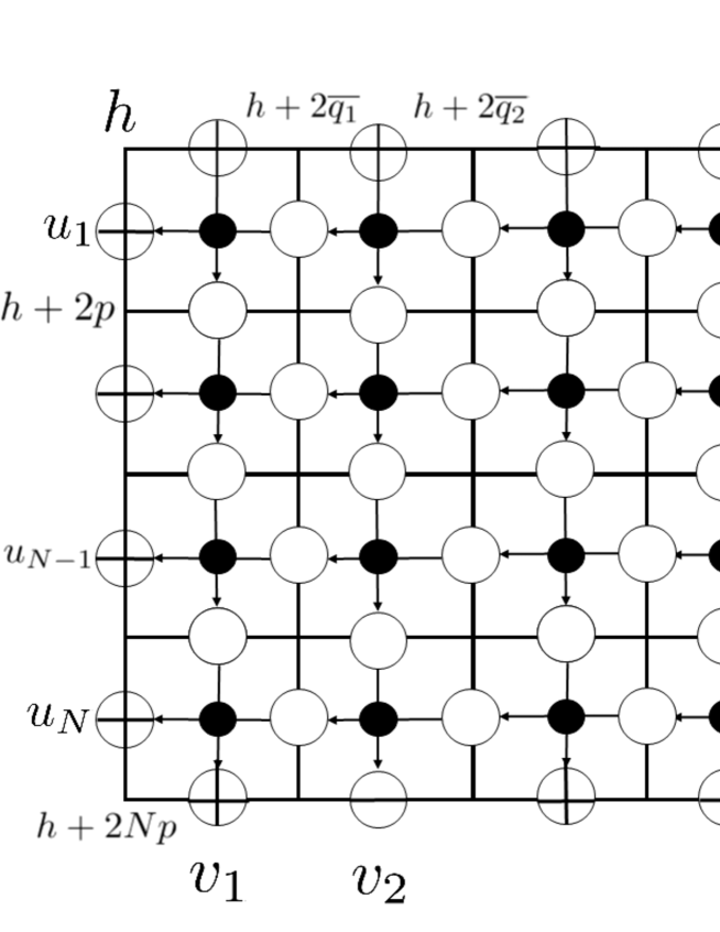
Figure 9: The wavefunctions $W_{M,N}(u_{1},\dots,u_{N}|v_{1},\dots,v_{M}|x_{1},\dots,x_{N}|h)$ (3.1). The figure illustrates the case $M=7$, $N=4$, $x_{1}=2$, $x_{2}=5$, $x_{3}=6$, $x_{4}=7$.

Figure 10: The wavefunctions $V_{M,N}(u_{1},\dots,u_{N}|v_{1},\dots,v_{M}|x_{1},\dots,x_{N}|h)$ (3.3). The figure illustrates the case $M=7$, $N=4$, $x_{1}=1$, $x_{2}=3$, $x_{3}=5$, $x_{4}=6$.

The wavefunctions (3.1), (3.3) can be explicitly expressed using deformed elliptic Vandermonde determinants and elliptic symmetric functions defined below.

Definition 3.1.

We define the following elliptic Schur function
$S_{M,N}(u_{1},\dots,u_{N}|v_{1},\dots,v_{M}|x_{1},\dots,x_{N}|h)$ which depends on the symmetric variables
$u_{1},\dots,u_{N}$, two sets of complex parameters $v_{1},\dots,v_{M}$ and $q_{1},\dots,q_{M}$, two complex parameters $h$, $p$ and integers $x_{1},\dots,x_{N}$ satisfying $1\leq x_{1}<\cdots<x_{N}\leq M$,

$$S_{M,N}(u_{1},\dots,u_{N}|v_{1},\dots,v_{M}|x_{1},\dots,x_{N}|h)$$

$$= \sum_{\sigma\in S_{N}}\prod_{1\leq j<k\leq N}\frac{1}{[u_{\sigma(j)}-u_{\sigma(k)}]}\prod_{j=1}^{N}\prod_{k=x_{j}+1}^{M}[u_{\sigma(j)}-v_{k}-q_{k}+p]$$

$$\times\prod_{j=1}^{N}\frac{[h+2jp+2\overline{q_{M}}]^{1/2}[2p]^{1/2}[2q_{x_{j}}]^{1/2}}{[h+2(j-1)p+2\overline{q_{M}}]^{1/2}[h+2Np+2\overline{q_{x_{j}-1}}]^{1/2}[h+2Np+2\overline{q_{x_{j}}}]^{1/2}}$$

$$\times\prod_{j=1}^{N}[-u_{\sigma(j)}+v_{x_{j}}+h+(2N-1)p+q_{x_{j}}+2\overline{q_{x_{j}-1}}]\prod_{j=1}^{N}\prod_{k=1}^{x_{j}-1}[u_{\sigma(j)}-v_{k}+p+q_{k}],$$ (3.5)

$$= \prod_{1\leq j<k\leq N}\frac{1}{[u_{j}-u_{k}]}\mathrm{det}_{N}(f_{x_{j}}(u_{k}|v_{1},\dots,v_{M})),$$ (3.6)

$$f_{x_{j}}(u|v_{1},\dots,v_{M})$$

$$= \frac{[h+2jp+2\overline{q_{M}}]^{1/2}[2p]^{1/2}[2q_{x_{j}}]^{1/2}}{[h+2(j-1)p+2\overline{q_{M}}]^{1/2}[h+2Np+2\overline{q_{x_{j}-1}}]^{1/2}[h+2Np+2\overline{q_{x_{j}}}]^{1/2}}$$

$$\times[-u+v_{x_{j}}+h+(2N-1)p+q_{x_{j}}+2\overline{q_{x_{j}-1}}]\prod_{k=1}^{x_{j}-1}[u-v_{k}+p+q_{k}]\prod_{k=x_{j}+1}^{M}[u-v_{k}+p-q_{k}].$$ (3.7)

Recall that $\overline{q_{j}}$ is defined as $\overline{q_{j}}=\sum_{k=1}^{j}q_{k}$.

We also define another elliptic Schur function $T_{M,N}(u_{1},\dots,u_{N}|v_{1},\dots,v_{M}|x_{1},\dots,x_{N}|h)$ which depends on the symmetric variables $u_{1},\dots,u_{N}$, two sets of complex parameters $v_{1},\dots,v_{M}$ and $q_{1},\dots,q_{M}$, two complex parameters $h$, $p$ and integers $x_{1},\dots,x_{N}$ satisfying $1\leq x_{1}<\cdots<x_{N}\leq M$,

$$T_{M,N}(u_{1},\dots,u_{N}|v_{1},\dots,v_{M}|x_{1},\dots,x_{N}|h)$$

$$= \sum_{\sigma\in S_{N}}\prod_{1\leq j<k\leq N}\frac{1}{[u_{\sigma(j)}-u_{\sigma(k)}]}\prod_{j=1}^{N}\prod_{k=x_{j}+1}^{M}[u_{\sigma(j)}-v_{k}+q_{k}+p]$$

$$\times\prod_{j=1}^{N}\frac{[h+2(j-1)p]^{1/2}[2p]^{1/2}[2q_{x_{j}}]^{1/2}}{[h+2jp]^{1/2}[h+2\overline{q_{x_{j}-1}}]^{1/2}[h+2\overline{q_{x_{j}}}]^{1/2}}$$

$$\times\prod_{j=1}^{N}[u_{\sigma(j)}-v_{x_{j}}+h+p+q_{x_{j}}+2\overline{q_{x_{j}-1}}]\prod_{j=1}^{N}\prod_{k=1}^{x_{j}-1}[u_{\sigma(j)}-v_{k}+p-q_{k}],$$ (3.8)

$$= \prod_{1\leq j<k\leq N}\frac{1}{[u_{j}-u_{k}]}\mathrm{det}_{N}(h_{x_{j}}(u_{k}|v_{1},\dots,v_{M})),$$ (3.9)

$$h_{x_{j}}(u|v_{1},\dots,v_{M})$$

$$= \frac{[h+2(j-1)p]^{1/2}[2p]^{1/2}[2q_{x_{j}}]^{1/2}}{[h+2jp]^{1/2}[h+2\overline{q_{x_{j}-1}}]^{1/2}[h+2\overline{q_{x_{j}}}]^{1/2}}$$

$$\times[u-v_{x_{j}}+h+p+q_{x_{j}}+2\overline{q_{x_{j}-1}}]\prod_{k=1}^{x_{j}-1}[u-v_{k}+p-q_{k}]\prod_{k=x_{j}+1}^{M}[u-v_{k}+p+q_{k}].$$ (3.10)

The wavefunctions of the elliptic Felderhof model can be expressed as products of one-parameter deformations of the elliptic Vandermonde determinant and the elliptic Schur functions $S_{M,N}(u_{1},\dots,u_{N}|v_{1},\dots,v_{M}|x_{1},\dots,x_{N}|h)$ and $T_{M,N}(u_{1},\dots,u_{N}|v_{1},\dots,v_{M}|x_{1},\dots,x_{N}|h)$ defined above. We present the correspondence below.

Theorem 3.2.

The wavefunctions of the elliptic Felderhof model
$W_{M,N}(u_{1},\dots,u_{N}|v_{1},\dots,v_{M}|x_{1},\dots,x_{N}|h)$ is explicitly expressed as the product of a one-parameter deformation of an elliptic Vandermonde determinant $\displaystyle\prod_{1\leq j<k\leq N}[u_{j}-u_{k}+2p]$ and the elliptic Schur functions $S_{M,N}(u_{1},\dots,u_{N}|v_{1},\dots,v_{M}|x_{1},\dots,x_{N}|h)$

$$W_{M,N}(u_{1},\dots,u_{N}|v_{1},\dots,v_{M}|x_{1},\dots,x_{N}|h)$$

$$= \prod_{1\leq j<k\leq N}[u_{j}-u_{k}+2p]S_{M,N}(u_{1},\dots,u_{N}|v_{1},\dots,v_{M}|x_{1},\dots,x_{N}|h).$$ (3.11)

The wavefunctions $V_{M,N}(u_{1},\dots,u_{N}|v_{1},\dots,v_{M}|x_{1},\dots,x_{N}|h)$ is explicitly expressed as the product of a one-parameter deformation of an elliptic Vandermonde determinant $\displaystyle\prod_{1\leq j<k\leq N}[u_{j}-u_{k}-2p]$ and the elliptic Schur functions $T_{M,N}(u_{1},\dots,u_{N}|v_{1},\dots,v_{M}|x_{1},\dots,x_{N}|h)$

$$V_{M,N}(u_{1},\dots,u_{N}|v_{1},\dots,v_{M}|x_{1},\dots,x_{N}|h)$$

$$= \prod_{1\leq j<k\leq N}[u_{j}-u_{k}-2p]T_{M,N}(u_{1},\dots,u_{N}|v_{1},\dots,v_{M}|x_{1},\dots,x_{N}|h).$$ (3.12)

The relation (3.11) is shown in [45]. In the Appendix, we give a proof of (3.12) in some detail.

Now, combining the determinant formula for the scalar products (Theorem 2.1) and the correspondence between the wavefunctions and the elliptic Schur functions (Theorem 3.2), one can derive the Cauchy formula for the elliptic Schur functions.

Theorem 3.3.

We have the following Cauchy formula for the elliptic Schur functions

$$\sum_{1\leq x_{1}<x_{2}<\cdots<x_{N}\leq M} S_{M,N}(u_{1},\dots,u_{N}|v_{1},\dots,v_{M}|x_{1},\dots,x_{N}|h)$$

$$\times T_{M,N}(w_{1},\dots,w_{N}|v_{1},\dots,v_{M}|x_{1},\dots,x_{N}|h+2Np)$$

$$= [2p]^{N}\frac{[h+2Np]^{1/2}[h+2Np+2\overline{q_{M}}]^{1/2}}{[h+4Np]^{1/2}[h+2\overline{q_{M}}]^{1/2}}\frac{1}{\prod_{1\leq j<k\leq N}[u_{j}-u_{k}][w_{j}-w_{k}]}$$

$$\times\mathrm{det}_{N}\Bigg{(}\frac{\frac{[w_{j}+h+2Np-u_{k}]}{[h+2Np]}a(w_{j})d(u_{k})-\frac{[w_{j}+h+2Np-u_{k}+2\overline{q_{M}}]}{[h+2Np+2\overline{q_{M}}]}a(u_{k})d(w_{j})}{[u_{k}-w_{j}]}\Bigg{)}.$$ (3.13)

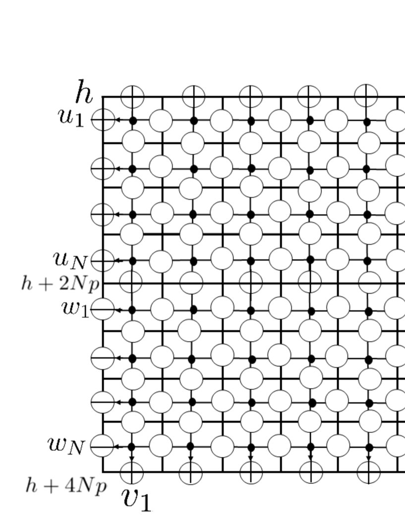
Figure 11: A graphical representation of a summand corresponding to $x_{1}=2$, $x_{2}=5$, $x_{3}=7$, $x_{4}=11$ in the decomposition of the scalar products into the sum over products of the wavefunctions (3.15).

Proof.

The scalar products (2.1) can be evaluated by inserting the completeness relation

$$\sum_{1\leq x_{1}<x_{2}<\cdots<x_{N}\leq M}|x_{1}\cdots x_{N}\rangle\langle x_{1}\cdots x_{N}|=\mathrm{Id},$$ (3.14)

and using the correspondence between the wavefunctions and the elliptic Schur functions (3.11), (3.12) in Theorem 3.2 as

$$Q_{M,N}(u_{1},\dots,u_{N}|w_{1},\dots,w_{N}|v_{1},\dots,v_{M}|h)$$

$$= {}_{M}\langle\Omega|C(w_{N}|v_{1},\dots,v_{M}|p|q_{1},\dots,q_{M}|h+2(2N-1)p)$$

$$\times\cdots\times C(w_{1}|v_{1},\dots,v_{M}|p|q_{1},\dots,q_{M}|h+2Np)$$

$$\times B(u_{N}|v_{1},\dots,v_{M}|p|q_{1},\dots,q_{M}|h+2(N-1)p)$$

$$\times\cdots\times B(u_{1}|v_{1},\dots,v_{M}|p|q_{1},\dots,q_{M}|h)|\Omega\rangle_{M},$$

$$= \sum_{1\leq x_{1}<x_{2}<\cdots<x_{N}\leq M}{}_{M}\langle\Omega|C(w_{N}|v_{1},\dots,v_{M}|p|q_{1},\dots,q_{M}|h+2(2N-1)p)$$

$$\times\cdots\times C(w_{1}|v_{1},\dots,v_{M}|p|q_{1},\dots,q_{M}|h+2Np)|x_{1}\cdots x_{N}\rangle$$

$$\times\langle x_{1}\cdots x_{N}|B(u_{N}|v_{1},\dots,v_{M}|p|q_{1},\dots,q_{M}|h+2(N-1)p)$$

$$\times\cdots\times B(u_{1}|v_{1},\dots,v_{M}|p|q_{1},\dots,q_{M}|h)|\Omega\rangle_{M},$$

$$= \sum_{1\leq x_{1}<x_{2}<\cdots<x_{N}\leq M}V_{M,N}(w_{1},\dots,w_{N}|v_{1},\dots,v_{M}|x_{1},\dots,x_{N}|h+2Np)$$

$$\times W_{M,N}(u_{1},\dots,u_{N}|v_{1},\dots,v_{M}|x_{1},\dots,x_{N}|h)$$

$$= \sum_{1\leq x_{1}<x_{2}<\cdots<x_{N}\leq M}\prod_{1\leq j<k\leq N}[w_{j}-w_{k}-2p]T_{M,N}(w_{1},\dots,w_{N}|v_{1},\dots,v_{M}|x_{1},\dots,x_{m}|h+2Np)$$

$$\times\prod_{1\leq j<k\leq N}[u_{j}-u_{k}+2p]S_{M,N}(u_{1},\dots,u_{N}|v_{1},\dots,v_{M}|x_{1},\dots,x_{N}|h).$$ (3.15)

See Figure 11 for a graphical description of the decomposition (3.15). The Cauchy formula for the elliptic Schur functions (3.13) follows from comparing (3.15) with the direct evaluation which gives the determinant formula for the scalar products (2.2) (Theorem 2.1).

∎

4 Conclusion

In this paper, we examined the scalar products of the elliptic Felderhof model introduced by Foda-Wheeler-Zuparic [30], which is an elliptic extension of the face-type Felderhof model [31] of Deguchi-Akutsu [32]. By applying the Izergin-Korepin technique developed by Wheeler [79] to analyze the scalar produts, we derived the determinant formula for the scalar products of the elliptic Felderhof model by constructing the explicit determinant forms of the intermediate scalar products, which connects the scalar products and the domain wall boundary partition functions.

The scalar products can be evaluated in another way as a sum over products of the wavefunctions. For the case of the elliptic Felderhof models, the wavefunctions are expressed as a deformed elliptic Vandermonde determinant and elliptic Schur functions, which can be shown for example by the recently-developed Izergin-Korepin technique to analyze the wavefunctions [43, 44, 45]. By combining this way of evaluation with the direct evaluation which gives the determinant formula, we obtained the Cauchy formula for the elliptic Schur functions.

For the case of trigonometric integrable models, other boundary conditions such as the reflecting boundaries, half-turn boundaries are investigated [52, 53, 54], where in some cases symplectic Schur functions emerge as the wavefunctions. There are also progresses on the introduction of a higher rank model called as the metaplectic ice [58], where connections with metaplectic Whittaker functions are established. It seems valuable to lift those works to the elliptic setting, which may lead to new developments in number theory as well as integrable models.

Appendix

In this Appendix, we give a proof of (3.12) in some detail, based on the idea initiated by Korepin [41], listing the properties of the domain wall boundary partition functions which uniquely characterize it. This characterization lead Izergin [42] to found the determinant representation (Izergin-Korepin determinant) of the domain wall boundary partition functions of the $U_{q}(sl_{2})$ six-vertex model. We recently extended the Izergin-Korepin technique to be able to analyze the wavefunctions [44, 45, 43]. We apply this technique here. As usual, we first list the properties which uniquely characterize the wavefunctions.

Proposition 4.1.

The wavefunctions $V_{M,N}(u_{1},\dots,u_{N}|v_{1},\dots,v_{M}|x_{1},\dots,x_{N}|h)$ satisfies the following properties.

(1) If $x_{N}=M$, the wavefunctions $V_{M,N}(u_{1},\dots,u_{N}|v_{1},\dots,v_{M}|x_{1},\dots,x_{N}|h)$ is an elliptic polynomial of $v_{M}$ in $\Theta_{N}(\chi)$.

(2) The wavefunctions $V_{M,N}(u_{\sigma}(1),\dots,u_{\sigma}(N)|v_{1},\dots,v_{M}|x_{1},\dots,x_{N}|h)$ with the ordering of the spectral parameters permuted $u_{\sigma(1)},\dots,u_{\sigma(N)}$, $\sigma\in S_{N}$ are related to the wavefunctions $V_{M,N}(u_{1},\dots,u_{N}|v_{1},\dots,v_{M}|x_{1},\dots,x_{N}|h)$ by the following relation

$$\prod_{\begin{subarray}{c}1\leq j<k\leq N\\ \sigma(j)>\sigma(k)\end{subarray}}[u_{\sigma(j)}-u_{\sigma(k)}-2p]V_{M,N}(u_{1},\dots,u_{N}|v_{1},\dots,v_{M}|x_{1},\dots,x_{N}|h)$$

$$= \prod_{\begin{subarray}{c}1\leq j<k\leq N\\ \sigma(j)>\sigma(k)\end{subarray}}[u_{\sigma(k)}-u_{\sigma(j)}-2p]V_{M,N}(u_{\sigma(1)},\dots,u_{\sigma(N)}|v_{1},\dots,v_{M}|x_{1},\dots,x_{N}|h).$$ (4.1)

(3) If $x_{N}=M$, the following recursive relations between the wavefunctions hold:

$$V_{M,N}(u_{1},\dots,u_{N}|v_{1},\dots,v_{M}|x_{1},\dots,x_{N}|h)|_{v_{M}=u_{N}+p+q_{M}}$$

$$= \frac{[2p]^{1/2}[2q_{M}]^{1/2}[h+2\overline{q_{M-1}}]^{1/2}[h+2(N-1)p]^{1/2}}{[h+2\overline{q_{M}}]^{1/2}[h+2Np]^{1/2}}\prod_{j=1}^{N-1}[u_{j}-u_{N}-2p]\prod_{j=1}^{M-1}[u_{N}-v_{j}+p-q_{j}]$$

$$\times V_{M-1,N-1}(u_{1},\dots,u_{N-1}|v_{1},\dots,v_{M-1}|x_{1},\dots,x_{N-1}|h).$$ (4.2)

If $x_{N}\neq M$, the following factorizations hold for the wavefunctions:

$$V_{M,N}(u_{1},\dots,u_{N}|v_{1},\dots,v_{M}|x_{1},\dots,x_{N}|h)$$

$$= \prod_{j=1}^{N}[u_{j}-v_{M}+q_{M}+p]V_{M-1,N}(u_{1},\dots,u_{N}|v_{1},\dots,v_{M-1}|x_{1},\dots,x_{N}|h).$$ (4.3)

(4) The following evaluation holds for the case $N=1$, $x_{1}=M$

$$V_{M,1}(u|v_{1},\dots,v_{M}|M|h)$$

$$= \frac{[h]^{1/2}[2p]^{1/2}[2q_{M}]^{1/2}[u-v_{M}+h+p+q_{M}+2\overline{q_{M-1}}]}{[h+2p]^{1/2}[h+2\overline{q_{M-1}}]^{1/2}[h+2\overline{q_{M}}]^{1/2}}\prod_{k=1}^{M-1}[u-v_{k}+p-q_{k}].$$ (4.4)

Proposition 4.1 can be proved in a similar way with the Proposition 2.2 for the scalar products. The next step is to find the explicit forms of the functions which satisfy all the properties in Proposition 4.1. This is given in the next proposition. The proof of the proposition also concludes the proof of (3.12).

Proposition 4.2.

The product of a deformed elliptic Vandermonde determinant and the elliptic Schur functions $\prod_{1\leq j<k\leq N}[u_{j}-u_{k}-2p]T_{M,N}(u_{1},\dots,u_{N}|v_{1},\dots,v_{M}|x_{1},\dots,x_{N}|h)$ satisfy all the properties listed in Proposition 4.1, which the wavefunctions of the elliptic Felderhof model $V_{M,N}(u_{1},\dots,u_{N}|v_{1},\dots,v_{M}|x_{1},\dots,x_{N}|h)$ must satisfy.

Proof.

This can be proved by showing that

$$H_{M,N}(u_{1},\dots,u_{N}|v_{1},\dots,v_{M}|x_{1},\dots,x_{N}|h)$$

$$:= \prod_{1\leq j<k\leq N}[u_{j}-u_{k}-2p]T_{M,N}(u_{1},\dots,u_{N}|v_{1},\dots,v_{M}|x_{1},\dots,x_{N}|h)$$

$$= \prod_{1\leq j<k\leq N}[u_{j}-u_{k}-2p]\sum_{\sigma\in S_{N}}\prod_{1\leq j<k\leq N}\frac{1}{[u_{\sigma(j)}-u_{\sigma(k)}]}\prod_{j=1}^{N}\prod_{k=x_{j}+1}^{M}[u_{\sigma(j)}-v_{k}+q_{k}+p]$$

$$\times\prod_{j=1}^{N}\frac{[h+2(j-1)p]^{1/2}[2p]^{1/2}[2q_{x_{j}}]^{1/2}}{[h+2jp]^{1/2}[h+2\overline{q_{x_{j}-1}}]^{1/2}[h+2\overline{q_{x_{j}}}]^{1/2}},$$

$$\times\prod_{j=1}^{N}[u_{\sigma(j)}-v_{x_{j}}+h+p+q_{x_{j}}+2\overline{q_{x_{j}-1}}]\prod_{j=1}^{N}\prod_{k=1}^{x_{j}-1}[u_{\sigma(j)}-v_{k}+p-q_{k}],$$ (4.5)

satisfies Properties (1), (2), (3) and (4) in Proposition 4.1. For example, Property (1) can be checked by computing the quasi-periodicities of $H_{M,N}(u_{1},\dots,u_{N}|v_{1},\dots,v_{M}|x_{1},\dots,x_{N-1},M|h)$ with respect to $v_{M}$, which are given by

$$H_{M,N}(u_{1},\dots,u_{N}|v_{1},\dots,v_{M}+1|x_{1},\dots,x_{N-1},M|h)$$

$$= (-1)^{N}H_{M,N}(u_{1},\dots,u_{N}|v_{1},\dots,v_{M}|x_{1},\dots,x_{N-1},M|h),$$ (4.6)

$$H_{M,N}(u_{1},\dots,u_{N}|v_{1},\dots,v_{M}-i\mathrm{log}({\bf q})/\pi|x_{1},\dots,x_{N-1},M|h)$$

$$= (-{\bf q}^{-1})^{N}\mathrm{exp}\Bigg{(}-2\pi i\Bigg{(}Nv_{M}-h-2\overline{q_{M-1}}-Nq_{M}-Np-\sum_{j=1}^{N}u_{j}\Bigg{)}\Bigg{)}$$

$$\times H_{M,N}(u_{1},\dots,u_{N}|v_{1},\dots,v_{M}|x_{1},\dots,x_{N-1},M|h).$$ (4.7)

These explicit quasi-periodicities shows that $H_{M,N}(u_{1},\dots,u_{N}|v_{1},\dots,v_{M}|x_{1},\dots,x_{N-1},M|h)$ is an elliptic polynomial of degree $N$ in $v_{M}$. Also, the factors $(-1)^{N}$ and $(-{\bf q}^{-1})^{N}\mathrm{exp}\Bigg{(}-2\pi i\Bigg{(}Nv_{M}-h-2\overline{q_{M-1}}-Nq_{M}-Np-\sum_{j=1}^{N}u_{j}\Bigg{)}\Bigg{)}$ in (4.6) and (4.7) are the same with the ones which appear when we examine the quasi-periodicities of the wavefunctions
$V_{M,N}(u_{1},\dots,u_{N}|v_{1},\dots,v_{M}|x_{1},\dots,x_{N-1},M|h)$ as a function of $v_{M}$.

Property (3) for the case $x_{N}=M$ can be shown as follows. The factors $\displaystyle\prod_{j=1}^{N-1}[u_{\sigma(j)}-v_{M}+q_{M}+p]$ in each summand in $H_{M,N}(u_{1},\dots,u_{N}|v_{1},\dots,v_{M}|x_{1},\dots,x_{N}|h)$ means that we only have to deal with the summands satisfying $\sigma(N)=N$ in (3.5) which survive after the substitution $v_{M}=u_{N}+p+q_{M}$. Then we find that $H_{M,N}(u_{1},\dots,u_{N}|v_{1},\dots,v_{M}|x_{1},\dots,x_{N}|h)$ evaluated at $v_{M}=u_{N}+p+q_{M}$ can be expressed using the symmetric group $S_{N-1}$ where every $\sigma^{\prime}\in S_{N-1}$ satisfies $\{\sigma^{\prime}(1),\cdots,\sigma^{\prime}(N-1)\}=\{1,\cdots,N-1\}$ as follows:

$$H_{M,N}(u_{1},\dots,u_{N}|v_{1},\dots,v_{M}|x_{1},\dots,x_{N}|h)|_{v_{M}=u_{N}+p+q_{M}}$$

$$= \prod_{1\leq j<k\leq N-1}[u_{j}-u_{k}-2p]\prod_{j=1}^{N-1}[u_{j}-u_{N}-2p]$$

$$\times\sum_{\sigma^{\prime}\in S_{N-1}}\prod_{1\leq j<k\leq N-1}\frac{1}{[u_{\sigma^{\prime}(j)}-u_{\sigma^{\prime}(k)}]}\prod_{j=1}^{N-1}\frac{1}{[u_{\sigma^{\prime}(j)}-u_{N}]}$$

$$\times\prod_{j=1}^{N-1}\prod_{k=x_{j}+1}^{M-1}[u_{\sigma^{\prime}(j)}-v_{k}+q_{k}+p]\prod_{j=1}^{N-1}[u_{\sigma^{\prime}(j)}-u_{N}]$$

$$\times\frac{[h+2(N-1)p]^{1/2}[2p]^{1/2}[2q_{M}]^{1/2}}{[h+2Np]^{1/2}[h+2\overline{q_{M-1}}]^{1/2}[h+2\overline{q_{M}}]^{1/2}}\prod_{j=1}^{N-1}\frac{[h+2(j-1)p]^{1/2}[2p]^{1/2}[2q_{x_{j}}]^{1/2}}{[h+2jp]^{1/2}[h+2\overline{q_{x_{j}-1}}]^{1/2}[h+2\overline{q_{x_{j}}}]^{1/2}}$$

$$\times[h+2\overline{q_{M-1}}]\prod_{j=1}^{N-1}[u_{\sigma^{\prime}(j)}-v_{x_{j}}+h+p+q_{x_{j}}+2\overline{q_{x_{j}-1}}]$$

$$\times\prod_{j=1}^{N-1}\prod_{k=1}^{x_{j}-1}[u_{\sigma^{\prime}(j)}-v_{k}+p-q_{k}]\prod_{k=1}^{M-1}[u_{N}-v_{k}+p-q_{k}].$$ (4.8)

After appropriately cancelling and rearraning the expression above, we find that (4.8) can be rewritten as

$$H_{M,N}(u_{1},\dots,u_{N}|v_{1},\dots,v_{M}|x_{1},\dots,x_{N}|h)|_{v_{M}=u_{N}+p+q_{M}}$$

$$= \frac{[2p]^{1/2}[2q_{M}]^{1/2}[h+2\overline{q_{M-1}}]^{1/2}[h+2(N-1)p]^{1/2}}{[h+2\overline{q_{M}}]^{1/2}[h+2Np]^{1/2}}\prod_{j=1}^{N-1}[u_{j}-u_{N}-2p]\prod_{j=1}^{M-1}[u_{N}-v_{j}+p-q_{j}]$$

$$\times\prod_{1\leq j<k\leq N-1}[u_{j}-u_{k}-2p]\sum_{\sigma^{\prime}\in S_{N-1}}\prod_{1\leq j<k\leq N-1}\frac{1}{[u_{\sigma^{\prime}(j)}-u_{\sigma^{\prime}(k)}]}$$

$$\times\prod_{j=1}^{N-1}\prod_{k=x_{j}+1}^{M-1}[u_{\sigma^{\prime}(j)}-v_{k}+q_{k}+p]\prod_{j=1}^{N-1}\frac{[h+2(j-1)p]^{1/2}[2p]^{1/2}[2q_{x_{j}}]^{1/2}}{[h+2jp]^{1/2}[h+2\overline{q_{x_{j}-1}}]^{1/2}[h+2\overline{q_{x_{j}}}]^{1/2}}$$

$$\times\prod_{j=1}^{N-1}[u_{\sigma^{\prime}(j)}-v_{x_{j}}+h+p+q_{x_{j}}+2\overline{q_{x_{j}-1}}]\prod_{j=1}^{N-1}\prod_{k=1}^{x_{j}-1}[u_{\sigma^{\prime}(j)}-v_{k}+p-q_{k}]$$

$$= \frac{[2p]^{1/2}[2q_{M}]^{1/2}[h+2\overline{q_{M-1}}]^{1/2}[h+2(N-1)p]^{1/2}}{[h+2\overline{q_{M}}]^{1/2}[h+2Np]^{1/2}}\prod_{j=1}^{N-1}[u_{j}-u_{N}-2p]\prod_{j=1}^{M-1}[u_{N}-v_{j}+p-q_{j}]$$

$$\times H_{M-1,N-1}(u_{1},\dots,u_{N-1}|v_{1},\dots,v_{M-1}|x_{1},\dots,x_{N-1}|h),$$ (4.9)

which is exactly the same with the one (4.2) for the wavefunctions of the elliptic Felderhof model $V_{M,N}(u_{1},\dots,u_{N}|v_{1},\dots,v_{M}|x_{1},\dots,x_{N}|h)$.

∎

Now that we have shown Proposition 4.2, we find that the elliptic function
$H_{M,N}(u_{1},\dots,u_{N}|v_{1},\dots,v_{M}|x_{1},\dots,x_{N}|h)$ is nothing but the explicit form of the wavefunctions $V_{M,N}(u_{1},\dots,u_{N}|v_{1},\dots,v_{M}|x_{1},\dots,x_{N}|h)$

$$V_{M,N}(u_{1},\dots,u_{N}|v_{1},\dots,v_{M}|x_{1},\dots,x_{N}|h)=H_{M,N}(u_{1},\dots,u_{N}|v_{1},\dots,v_{M}|x_{1},\dots,x_{N}|h),$$ (4.10)

hence (3.12) in Theorem 3.2 is proved.

References

- [1] G. Felder, Elliptic quantum groups, Proceedings of the XIth International Congress of Mathematical Physics (Paris, 1994) (International Press, Boston, MA, 1995), pp. 211-218
- [2] G. Felder and A. Varchenko, On representations of the elliptic quantum groups , Commun. Math. Phys. 181 (1996) 741
- [3] H. Konno, An Elliptic Algebra and the Fusion RSOS Model, Commun. Math. Phys. 195 (1998) 373
- [4] M. Jimbo, H. Konno, S. Odake and J. Shiraishi, Quasi-Hopf twistors for elliptic quantum groups, J. Trans. Groups 4 (1999) 303
- [5] L.D. Faddeev, E.K. Sklyanin and L.A. Takhtajan, The quantum inverse problem method. 1, Theor. Math. Phys. 40 (1980) 688
- [6] V. Drinfeld, Hopf algebras and the quantum Yang-Baxter equation, Sov. Math. Dokl. 32 (1985) 254
- [7] M. Jimbo, A -difference analogue of and the Yang-Baxter equation, Lett. Math. Phys. 10 (1985) 63
- [8] R.J. Baxter, Exactly Solved Models in Statistical Mechanics (Academic Press, London) (1982)
- [9] R.J. Baxter, Partition function of the eight-vertex lattice model, Ann. Phys. 70 (1972) 193
- [10] G.E. Andrews, R.J. Baxter and P.J. Forrester, Eight-vertex SOS model and generalized Rogers-. Ramanujan-type identities, J. Stat. Phys. 35 (1984) 193
- [11] M. Jimbo, T. Miwa and M. Okado, Solvable lattice models whose states are dominant integral weights of , Lett. Math. Phys. 14 (1987) 123
- [12] E. Date, M. Jimbo, A. Kuniba, T. Miwa and M. Okado, Exactly solvable SOS models: Local height probabilities and theta function identities, Nucl. Phys. B 290 (1987) 231
- [13] S. Pakuliak, V. Rubtsov and A. Silantyev, The SOS model partition function and the elliptic weight functions, J. Phys. A:Math. Theor. 41 (2008) 295204
- [14] H. Rosengren, An Izergin-Korepin-type identity for the 8VSOS model, with applications to alternating sign matrices, Adv. Appl. Math. 43 (2009) 137
- [15] W-L. Yang and Y-Z. Zhang, Partition function of the eight-vertex model with domain wall boundary condition, J. Math. Phys. 50 (2009) 083518
- [16] G. Filali and N. Kitanine, Partition function of the trigonometric SOS model with reflecting end, J. Stat. Phys. 1006 (2010) L06001
- [17] W-L. Yang, X. Chen, J. Feng, K. Hao, K.-J. Shi, C.-Y. Sun, Z.-Y. Yang and Y-Z. Zhang, Domain wall partition function of the eight-vertex model with a non-diagonal reflecting end, Nucl. Phys. B 847 (2011) 367
- [18] W-L. Yang, X. Chen, J. Feng, K. Hao, K.-J. Shi, C.-Y. Sun, Z.-Y. Yang and Y-Z. Zhang, Scalar products of the open XYZ chain with non-diagonal boundary terms, Nucl. Phys. B 848 (2011) 523
- [19] W. Galleas, Multiple integral representation for the trigonometric SOS model with domain wall boundaries, Nucl. Phys. B 858 (2012) 117
- [20] W. Galleas, Refined functional relations for the elliptic SOS model, Nucl. Phys. B 867 (2013) 855
- [21] W. Galleas and J. Lamers, Reflection algebra and functional equations, Nucl. Phys. B 886 (2014) 1003
- [22] J. Lamers, Integral formula for elliptic SOS models with domain walls and a reflecting end, Nucl. Phys. B 901 (2015) 556
- [23] H. Konno, Elliptic Weight Functions and Elliptic -KZ Equation, J. Integrable Systems 2 (2017) xyx011
- [24] A. Borodin, Symmetric elliptic functions, IRF models, and dynamic exclusion processes, arXiv:1701.05239
- [25] G. Felder, R. Rimanyi and A. Varchenko, Elliptic dynamical quantum groups and equivariant elliptic cohomology, arXiv:1702.08060
- [26] R. Rimanyi, V. Tarasov and A. Varchenko, Elliptic and K-theoretic stable envelopes and Newton polytopes, arXiv:1705.09344
- [27] V.E. Korepin, N.M. Bogoliubov and A.G. Izergin, Quantum Inverse Scattering Method and Correlation functions (Cambridge University Press, Cambridge) (1993)
- [28] N. Reshetikhin, Lectures on integrable models in statistical mechanics. In: Exact Methods in Low Dimensional Statistical Physics and Quantum Computing, Proceedings of Les Houches School in Theoretical Physics. (Oxford University Press, Oxford) (2010)
- [29] M. Jimbo and T. Miwa. Algebraic Analysis of Solvable Lattice Models volume 85 of CBMS Regional Conference Series in Mathematics. (American Mathematical Society, Providence, RI) (1995)
- [30] O. Foda, M. Wheeler and M. Zuparic, Two elliptic height models with factorized domain wall partition functions, J. Stat. Mech. 2008 (2008) P02001
- [31] B. Felderhof, Direct diagonalization of the transfer matrix of the zero-field free-fermion model, Physica 65 (1973) 421
- [32] T. Deguchi and Y. Akutsu, Colored Vertex Models, Colored IRF Models and Invariants of Trivalent Colored Graphs, J. Phys. Soc. Jpn. 62 (1993) 19
- [33] M. Okado, Solvable face models related to the Lie superalgebra , Lett. Math. Phys. 22 (1991) 39
- [34] T. Deguchi and A. Fujii, IRF models associated with representations of Lie superalgebras and , Mod. Phys. Lett. A 6 (1991) 3413
- [35] T. Deguchi and P. Martin, An Algebraic Approach to Vertex Models and Transfer Matrix Spectra, Int. J. Mod. Phys. A 7 Suppl. 1A (1992) 165
- [36] J-H-H. Perk and C.L. Schultz, New families of commuting transfer matrices in -state vertex models, Phys. Lett. A 84 (1981) 407
- [37] B. Brubaker, D. Bump and S. Friedberg, Schur Polynomials and the Yang-Baxter equation, Commun. Math. Phys. 308 (2011) 281
- [38] T. Tokuyama, A generating function of strict Gelfand patterns and some formulas on characters of general linear groups, J. Math. Soc. Japan 40 (1988) 671
- [39] H. Yamane, On defining relations of the affine Lie superalgebras and their quantized universal enveloping superalgebras, Publ. Res. Inst. Math. Sci. 35 (1999) 321
- [40] J. Murakami, The free-fermion model in presence of field related to the quantum group of affine type and the multi-variable Alexander polynomial of links, Infinite analysis. Adv. Ser. Math. Phys. 16B (1991) 765
- [41] V.E. Korepin, Calculation of norms of Bethe wave functions, Commun. Math. Phys. 86 (1982) 391
- [42] A. Izergin, Partition function of the six-vertea model in the finite volume, Sov. Phys. Dokl. 32 (1987) 878
- [43] K. Motegi, Izergin-Korepin analysis on the projected wavefunctions of the generalized free-fermion model, Adv. Math. Phys. Article ID 7563781 (2017)
- [44] K. Motegi, Elliptic supersymmetric integrable model and multivariable elliptic functions, Prog. Theo. Exp. Phys. 2017 (2017) 123A01
- [45] K. Motegi, Symmetric functions and wavefunctions of the six-vertex model and elliptic Felderhof model, preprint.
- [46] M. Schlosser, gElliptic h enumeration of nonintersecting lattice paths, J. Comb. Th. A. 114 (2007) 505
- [47] M. Noumi, Remarks on elliptic Schur functions, http://www.lorentzcenter.nl/lc/web/2010/423/presentations/Noumi.pdf
- [48] M. Noumi, Elliptic Askey-Wilson functions and associated elliptic Schur functions, http://www.lorentzcenter.nl/lc/web/2013/541/presentations/Noumi.pdf
- [49] S. Okada, Alternating sign matrices and some deformations of weyl’s denominator formulas, J. Algebraic Comb. 2 (1993) 155
- [50] A. Hamel and R.C. King, Symplectic shifted tableaux and deformations of Weyl’s denominator formula for , J. Algebraic Comb. 16 (2002) 269
- [51] A. Hamel and R.C. King, U-turn Alternating Sign Matrices, Symplectic Shifted Tableaux and Their Weighted Enumeration, J. Algebraic Comb. 21 (2005) 395
- [52] D. Ivanov, Symplectic Ice. in: Multiple Dirichlet series, -functions and automorphic forms, vol 300 of Progr. Math. Birkhäuser/Springer, New York, 205-222 (2012)
- [53] B. Brubaker, D. Bump, G. Chinta and P.E. Gunnells, Metaplectic Whittaker Functions and Crystals of Type B. in: Multiple Dirichlet series, -functions and automorphic forms, vol 300 of Progr. Math. Birkhäuser/Springer, New York, 93-118 (2012)
- [54] S.J. Tabony, Deformations of characters, metaplectic Whittaker functions and the Yang-Baxter equation, PhD. Thesis, Massachusetts Institute of Technology, USA (2011)
- [55] D. Bump, P. McNamara and M. Nakasuji, Factorial Schur functions and the Yang-Baxter equation, Comm. Math. Univ. St. Pauli 63 (2014) 23
- [56] A.M. Hamel and R.C. King, Tokuyama’s identity for factorial Schur and functions, Elect. J. Comb. 22 (2015) 2, P2.42
- [57] B. Brubaker and A. Schultz, The 6-vertex model and deformations of the Weyl character formula, J. Alg. Comb. 42 (2015) 917
- [58] B. Brubaker, V. Buciumas and D. Bump, A Yang-Baxter equation for metaplectic ice, arXiv:1604.02206
- [59] K. Motegi, Dual wavefunction of the Felderhof model, Lett. Math. Phys. 107 (2017) 1235
- [60] S-U. Zhao and Y-Z. Zhang, Supersymmetric Vertex Models with Domain Wall Boundary Conditions, J. Math. Phys. 48 (2007) 023504
- [61] O. Foda, A.D. Caradoc, M. Wheeler and M.L. Zuparic, On the trigonometric Felderhof model with domain wall boundary conditions, J. Stat. Mech. 0703 (2007) P03010
- [62] S-Y. Zhao, W-L. Yang and Y-Z. Zhang, Determinant Representation of Correlation Functions for the Free Fermion Model J. Math. Phys. 47 (2006) 013302
- [63] M. Wheeler, Free fermions in classical and quantum integrable models PhD thesis, Department of Mathematics and Statistics, The University of Melbourne, arXiv:1110.6703
- [64] M. Zuparic, Studies in integrable quantum lattice models and classical hierarchies Ph.D. Thesis, Department of Mathematics and Statistics, The University of Melbourne, arXiv:0908.3936
- [65] N.M. Bogoliubov, Boxed Plane Partitions as an Exactly Solvable Boson Model, J. Phys. A: Math. Gen. 38 (2005) 9415
- [66] D. Betea, M. Wheeler and P. Zinn-Justin, Refined Cauchy/Littlewood identities and six-vertex model partition functions: II. Proofs and new conjectures, J. Alg. Comb. 42 (2015) 555
- [67] D. Betea and M. Wheeler, Refined Cauchy and Littlewood identities, plane partitions and symmetry classes of alternating sign matrices, J. Comb. Th. Ser. A 137 (2016) 126
- [68] M. Wheeler and P. Zinn-Justin, Refined Cauchy/Littlewood identities and six-vertex model partition functions: III. Deformed bosons, Adv. Math. 299 (2016) 543
- [69] J.F. van Diejen and E. Emsiz, Orthogonality of Bethe Ansatz eigenfunctions for the Laplacian on a hyperoctahedral Weyl alcove, Commun. Math. Phys. 350 (2017) 1017
- [70] K. Motegi and K. Sakai, Vertex models, TASEP and Grothendieck polynomials, J. Phys. A: Math. Theor. 46 (2013) 355201
- [71] K. Motegi, Combinatorial properties of symmetric polynomials from integrable vertex models in finite lattice, J. Math. Phys. 58 (2017) 091703
- [72] K. Motegi and K. Sakai, -theoretic boson-fermion correspondence and melting crystals, J. Phys. A: Math. Theor. 47 (2014) 445202
- [73] C. Korff and C. Stroppel, The -WZNW Fusion Ring: a combinatorial construction and a realisation as quotient of quantum cohomology, Adv. Math. 225 (2010) 200
- [74] C. Korff, Quantum cohomology via vicious and osculating walkers, Lett. Math. Phys. 104 (2014) 771
- [75] A.Borodin, On a family of symmetric rational functions, Adv. in Math. 306 (2017) 973
- [76] A. Borodin and L. Petrov, Higher spin six vertex model and symmetric rational functions, Sel. Math. New Ser. 1 (2016)
- [77] Y. Takeyama, A deformation of affine Hecke algebra and integrable stochastic particle system, J. Phys. A 47 (2014) 465203
- [78] Y. Takeyama, On the eigenfunctions for the multi-species -Boson system, arXiv:1606.00578
- [79] M. Wheeler, An Izergin-Korepin procedure for calculating scalar products in six-vertex models, Nucl. Phys. B 852 (2011) 468
- [80] N.A. Slavnov, Calculation of scalar products of wave functions and form factors in the framework of the algebraic Bethe ansatz, Theor. Math. Phys. 79 (1989) 1605
- [81] G. Felder and A. Schorr, Separation of variables for quantum integrable systems on elliptic curves, J. Phys. A: Math.Gen. 32 (1999) 8001