Telling apart Felidae and Ursidae from the distribution of nucleotides in mitochondrial DNA

Abstract

Rank–frequency distributions of nucleotide sequences in mitochondrial DNA are defined in a way analogous to the linguistic approach, with the highest-frequent nucleobase serving as a whitespace. For such sequences, entropy and mean length are calculated. These parameters are shown to discriminate the species of the Felidae (cats) and Ursidae (bears) families. From purely numerical values we are able to see in particular that giant pandas are bears while koalas are not. The observed linear relation between the parameters is explained using a simple probabilistic model. The approach based on the nonadditive generalization of the Bose-distribution is used to analyze the frequency spectra of the nucleotide sequences. In this case, the separation of families is not very sharp. Nevertheless, the distributions for Felidae have on average longer tails comparing to Ursidae

Key words: Complex systems; rank–frequency distributions; mitochondrial DNA.

PACS numbers: 89.20.-a; 87.18.-h; 87.14.G-; 87.16.Tb

1 Introduction

Approaches of statistical physics proved to be efficient tools for studies of systems of different nature containing many interacting agents. Applications cover a vast variety of subjects, from voting models [1, 2], language dynamics [3, 4], and wealth distribution [5] to dynamics of infection spreading [6] and cellular growth [7].

Studies of deoxyribonucleic acid (DNA) and genomes are of particular interest as they can bridge several scientific domains, namely, biology, physics, and linguistics [8, 9, 10, 11, 12]. Such an interdisciplinary nature of the problem might require a brief introductory information as provided below.

DNA molecule is composed of two polynucleotide chains (called stands) containing four types of nucleotide bases: adenine (A), cytosine (C), guanine (G), and thymine (T) [13, p. 175]. The bases attached to a phosphate group form nucleotides. Nucleotides are linked by covalent bonds within a strand while there are hydrogen bonds between strands (A links T and C links with G) forming base pairs (bp). Typically, DNA molecules count millions to hundred millions base pairs.

Mitochondrial DNA (mtDNA) is a closed-circular, double-stranded molecule containing, in the case of mammals, 16–17 thousand base pairs [14]. It is thought to have bacterial evolutionary origin, so mtDNA might be considered as a nearly universal tool to study all eukaryotes. Mitochondrial DNA of animals is mostly inherited matrilineally and encodes the same gene content [15]. Due to quite short mtDNA sizes of different organisms, it is not easy to collect reliable statistical data for typical nucleotide sequences, like genes or even codons containing three bases.

Power-law distributions characterize rank–frequency relations of various units. Originally observed by Estoup in French [16] and Condon in English [17] and better known from the works of Zipf [18, 19], such a dependence is observed not only in linguistics [20, 21, 22, 23, 24] but for complex systems in general [25, 26] as manifested in urban development [27, 28, 29], income distribution [5, 30], genome studies [8, 31, 32], and other domains [33, 34].

The aim of this paper is to propose a simple approach based on frequency studies of nucleotide sequences in mitochondrial DNA, which would make it possible to define a set of parameters separating biological families and genera. The analysis is made for two carnivoran families of mammals, Felidae (including cats) [35] and Ursidae (bears) [36]. Applying the proposed approach, we are able to discriminate the two families and also draw conclusions whether some other species belong to these families or not.

The paper is organized as follows. In Section 2, the nucleotide sequences used in further analysis are defined. Section 3 contains the analysis based on rank–frequency distributions of these nucleotide sequences. In Section 4, a simple model is suggested to describe the observed frequency data and relations between the respective parameters. Frequency spectra corresponding to rank–frequency distributions are analyzed in Section 5. Conclusions are given in Section 6.

2 Nucleotide sequences

The four nucleobases forming mtDNA are the following compounds:

Adenine (C₅H₅N₅): [:-36]*5(-N(-H)-*6(-N=-N=(-NH_2)–)–N=)

Cytosine (C₄H₅N₃O): H-[:30]N*6(-(=O)-N=(-NH_2)-=-)

Thymine (C₅H₆N₂O₂): H-[:30]N*6(-(=O)-N(-H)-(=O)-(-CH_3)=-)

Guanine (C₅H₅N₅O): [:-36]*5(-N(-H)-*6(-N=(-NH_2)-N(-H)-(=O)–)–N=)

In Table 1, the information is given about the absolute and relative frequency of each nucleotide in mtDNA of the species analyzed in this work. The data are collected from databases of The National Center for Biotechnology Information [37].

Table 1: Distribution of nucleobases in species

Name		Size,	A		C		T		G
Latin	(common)	bp	abs.	rel.	abs.	rel.	abs.	rel.	abs.	rel.
Felidae:
Acinonyx jubatus	(cheetah)	17047	5642	0.331	4397	0.258	4693	0.275	2315	0.136
Felis catus	(domestic cat)	17009	5543	0.326	4454	0.262	4606	0.271	2406	0.141
Leopardus pardalis	(ocelot)	16692	5493	0.329	4454	0.267	4457	0.267	2288	0.137
Lynx lynx	(European lynx)	17046	5509	0.323	4615	0.271	4488	0.263	2434	0.143
Panthera leo	(lion)	17054	5448	0.319	4520	0.265	4608	0.270	2478	0.145
Panthera onca	(jaguar)	17049	5447	0.319	4509	0.264	4627	0.271	2466	0.145
Panthera pardus	(leopard)	16964	5397	0.318	4508	0.266	4592	0.271	2467	0.145
Panthera tigris	(tiger)	16990	5418	0.319	4513	0.266	4581	0.270	2478	0.146
Puma concolor	(puma)	17153	5643	0.329	4456	0.260	4685	0.273	2369	0.138
Ursidae:
Ailuropoda melanoleuca	(giant panda)	16805	5338	0.318	4000	0.238	4949	0.294	2518	0.150
Helarctos malayanus	(sun bear)	16783	5232	0.312	4295	0.256	4678	0.279	2578	0.154
Melursus ursinus	(sloth bear)	16817	5184	0.308	4364	0.259	4619	0.275	2650	0.158
Tremarctos ornatus	(spectacled bear)	16762	5246	0.313	4348	0.259	4583	0.273	2585	0.154
Ursus americanus	(Am. black bear)	16841	5244	0.311	4223	0.251	4760	0.283	2614	0.155
Ursus arctos	(brown bear)	17020	5258	0.309	4355	0.256	4731	0.278	2676	0.157
Ursus maritimus	(polar bear)	17017	5253	0.309	4346	0.255	4726	0.278	2692	0.158
Ursus spelaeus	(cave bear)	16780	5272	0.314	4256	0.254	4703	0.280	2549	0.152
Ursus thibetanus	(Asian black bear)	16794	5234	0.312	4284	0.255	4683	0.279	2593	0.154
Other:
Ailurus fulgens	(red panda)	16493	5426	0.329	4001	0.243	4863	0.295	2203	0.134
Phascolarctos cinereus	(koala)	16357	5854	0.358	4144	0.253	4501	0.275	1858	0.114
Drosophila melanogaster	(drosophila)	19517	8152	0.418	2003	0.103	7883	0.404	1479	0.076

Note the highest frequency of adenine in mtDNA for all species from Table 1. There is a well-known linguistic analogy for between distribution of DNA units [38, 39]. The “alphabet” can be defined as a set of four nucleobases or 24 aminoacids. In the present paper, we will not advance to further levels of “linguistic” organization of DNA [39] but introduce a new one in a way similar to [40]. This is done in the following fashion: as adenine is the most frequent nucleobase, one can treat it as a whitespace separating sequences of other nucleobases (C, T, and G). While a special role of adenine might be attributed to oxygen missing in its structure formula (given at the beginning of this Section), neither this nor other arguments dealing with specific nucleobase properties will be considered in the proposed approach, which is aimed to be a simple frequency-based analysis. For convenience, an empty element (between two As) will be denoted as ‘X’. So, the sequence from the mtDNA of Ailuropoda melanoleuca (giant panda)

ATACTATAAATCCACCTCTCATTTTATTCACTTCATACATGCTATTACAC

translates to

X T CT T X X TCC CCTCTC TTTT TTC CTTC T C TGCT TT C C

The obtained “words” (sequences between spaces) are the units for the analysis in the present work.

3 Analysis of rank–frequency dependences

The rank–frequency dependence is compiled for the defined nucleobase sequences in a standard way, so that the most frequent unit has rank 1, the second most frequent unit has rank 2 and so on. Units with equal frequencies are arbitrarily ordered within a consecutive range of ranks. Samples are shown in Table 2.

Table 2: Rank–frequency list for some species

rank	Felis catus		Panthera leo		A. melanoleuca		Ursus arctos
$r$	seq.	$f_{r}$	seq.	$f_{r}$	seq.	$f_{r}$	seq.	$f_{r}$
1	X	1725	X	1691	X	1241	X	1586
2	C	483	T	484	T	483	T	410
3	T	478	C	449	C	365	C	375
4	G	216	G	200	G	220	G	214
5	CT	179	CT	170	CT	186	CT	165
6	TT	163	TT	145	TT	178	TC	138
7	TC	143	TC	137	TC	118	TT	134
8	CC	116	CC	117	TG	99	TG	101
9	TG	99	TG	93	GC	92	CC	92
10	GC	81	GC	89	GT	84	GT	86
11	GG	79	GG	81	GG	83	GC	85
12	GT	78	GT	69	CC	82	GG	85
13	CG	48	CGT	53	CG	44	CGC	67
14	CCC	39	CG	45	CTT	44	CGTGT	53
15	CCT	38	CCC	39	TTT	43	CG	45
16	CGT	38	CCT	35	CCT	41	TTT	44
17	GCC	37	GCC	34	GCT	35	CTT	35
18	TTT	36	CTC	33	CGTGT	34	GCT	35
19	TCT	32	TTC	33	TCC	32	TCC	33
20	CTT	31	TTT	31	TCT	30	CTC	31
21	CTC	30	GCT	30	TTC	30	TTC	29
22	GCT	30	CTT	29	GCC	28	CCT	28
23	TCC	26	TCT	27	CGC	26	TCT	28
24	TCCT	24	TGT	23	CTC	25	GCC	26
25	TGT	23	TCC	22	GTT	24	CCC	25

The rank–frequency dependences follow Zipf’s law very precisely (see Fig. 1), so they can be modeled by

$$f_{r}=\frac{C}{r^{\alpha}}.$$ (1)

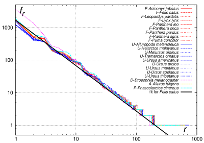
Figure 1: Rank–frequency dependence.

The normalization condition

$$\sum_{r}f_{r}=\sum_{r=1}^{\infty}\frac{C}{r^{\alpha}}=N$$ (2)

yields

$$C=\frac{N}{\zeta(\alpha)},$$ (3)

where $\zeta(\alpha)$ is Riemann’s zeta-function.

Entropy $S$ can be defined in a standard way,

$$S=-\sum_{r}p_{r}\ln p_{r},$$ (4)

where relative frequency $p_{r}=f_{r}/N$ and the summation runs over all the ranks.

After simple manipulations we obtain the following expression for entropy:

$$S=\ln\zeta(\alpha)-\alpha\frac{\zeta^{\prime}(\alpha)}{\zeta(\alpha)},$$ (5)

where the sum

$$\sum_{r=1}^{\infty}\frac{\ln r}{r^{\alpha}}=-\zeta^{\prime}(\alpha).$$ (6)

Due to a weak convergence ($1<\alpha<2$) it might be reasonable to consider finite summations over $r$ and hence the incomplete zeta-functions

$$\sum_{r=1}^{R}\frac{1}{r^{\alpha}} =\zeta(\alpha)-\zeta(\alpha,R+1),$$ (7)

$$\sum_{r=1}^{R}\frac{\ln r}{r^{\alpha}} =-\zeta^{\prime}(\alpha)+\zeta_{\alpha}(\alpha,R+1),$$ (8)

where

$$\zeta_{\alpha}(\alpha,R+1)\equiv\frac{\partial\zeta(\alpha,R+1)}{\partial\alpha}.$$ (9)

In this case, the entropy equals

$$S=\ln[\zeta(\alpha)-\zeta(\alpha,R+1)]-\alpha\frac{\zeta^{\prime}(\alpha)-\zeta_{\alpha}(\alpha,R+1)}{\zeta(\alpha)-\zeta(\alpha,R+1)}.$$ (10)

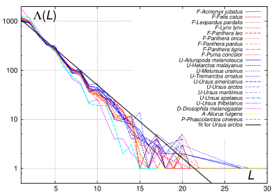
Figure 2: Sequence lengths. The first capital letter before the hyphen serves to distinguish families.

Mean sequence length

$$\langle L\rangle=\frac{1}{N}\sum_{L}L\Lambda(L).$$ (11)

The length distribution $\Lambda(L)$ can be approximately treated as a linear dependence in log-linear plot (see Fig. 2), so

$$\ln\Lambda(L)=-KL+B.$$ (12)

Applying the normalization condition

$$\sum_{L=0}^{\infty}\Lambda(L)=N$$ (13)

we obtain

$$\Lambda(L)=N\left(1-e^{-K}\right)e^{-KL}$$ (14)

and

$$\langle L\rangle=\frac{1}{e^{K}-1}\simeq\frac{1}{K},$$ (15)

the latter approximation corresponding to $K\ll 1$.

As shown in Fig. 3, the values of $S$ and $\langle L\rangle$ concentrate along a straight line,

$$\langle L\rangle=kS+b,\quad\textrm{with}\quad k=0.924\pm 0.015,\ \ b=-1.32\pm 0.06.$$ (16)

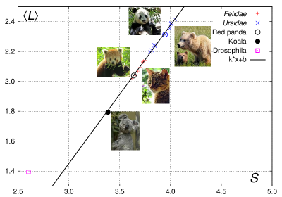
Figure 3: Entropy $S$ and mean length $\langle L\rangle$ for families and species analyzed in the present work.

Images in Fig. 3 serve to illustrate partial results dealing with some popular misbeliefs about bears. First of all, one clearly sees a large distance between bears and koala. The latter is known also as koala bear [41] or marsupial bear in many languages; the genus name (Phascolarctos) itself is composed of Greek words $\varphi\acute{\alpha}\sigma\kappa\omega\lambda o\varsigma$ ‘leathern bag’ and ’$\!\!\acute{\alpha}\rho\kappa\tau o\varsigma$ ‘bear’ [42, p. 529]. Despite the name and appearance, koalas are clearly not bears. On the other hand, we are able to confirm that giant pandas are bears and red pandas belong to a different genus. It would be incorrect however to place red pandas within Felidae based solely on the parameter values. Out of sheer curiosity, note some local names for pandas in Nepali bhālu birālō and Chinese xióngmāo meaning ‘bear-cat’, cf. [43, p. 143] and [44, p. 12].

Another pair of parameters to distinguish the Felidae and Ursidae families can be chosen from Table 1. It is clearly seen that the relative frequency of guanine $p_{\rm G}$ is a good discriminating parameter. The pairs of entropy $S$ and $p_{\rm G}$ are plotted in Fig. 4.

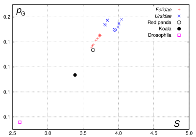
Figure 4: Entropy $S$ and relative frequency of guanine $p_{\rm G}$ for families and species analyzed in the present work.

The data for a model organism in biological studies, Drosophila melanogaster or common fruit fly, are shown for comparison and future references. We can observe that the parameters for this species differ significantly from those of the analyzed mammals. It can be considered as another confirmation that the proposed parameters can serve to distinguish families and genera.

4 Random model

Assuming that the chain of nucleotides forming the mitochondrial DNA is long enough, one can propose the following simplified model for the distribution of the defined nucleotide sequences. As seen from Table 1, relative frequencies of cytosine and thymine are nearly equal, the frequency of adenine is slightly larger, and the frequency of guanine is about twice smaller than that of cytosine or thymine. So, let the probability to find cytosine and thymine

$$p_{\rm C}=p_{\rm T}=p,$$ (17)

for adenine,

$$p_{\rm A}=(1+a)p,\qquad a>0.$$ (18)

and for guanine

$$p_{\rm G}=\frac{1}{2}p.$$ (19)

The normalization condition yields

$$p=\frac{2}{7+2a}.$$ (20)

So, for a Markovian chain (i.e., a randomly generated sequence) we have the probabilities to find

an empty element X:	$p_{\rm A}p_{\rm A}=(1+a)^{2}p^{2}$
a single nucleotide:	$p_{\rm A}p_{\rm C}p_{\rm A}=p_{\rm A}p_{\rm T}p_{\rm A}=p_{\rm A}^{2}p,\quad p_{\rm A}p_{\rm G}p_{\rm A}=\frac{1}{2}p_{\rm A}^{2}p$
CC, CT, TC, TT:	$p_{\rm A}^{2}p^{2}$
CG, GC, TG, GC:	$\frac{1}{2}p_{\rm A}^{2}p^{2}$
GG:	$\frac{1}{4}p_{\rm A}^{2}p^{2}$
CCC, CCT, …:	$p_{\rm A}^{2}p^{3}$
and so on.

For simplicity, we will further give all the probabilities relative the the highest value $p_{\rm A}^{2}=(1+a)^{2}p^{2}$.

It is easy to show that the function $\Lambda(L)$ up to a constant factor $\Lambda_{0}$ equals

$L$	$\Lambda(L)$
0	$\Lambda_{0}\cdot 1$
1	$\displaystyle\Lambda_{0}\left(2p+\frac{1}{2}p\right)$
2	$\displaystyle\Lambda_{0}\left(4p^{2}+4\cdot\frac{1}{2}p^{2}+\frac{1}{4}p^{2}\right)$
3	$\displaystyle\Lambda_{0}\left(8p^{3}+12\cdot\frac{1}{2}p^{2}+6\cdot\frac{1}{4}p^{2}+\frac{1}{8}p^{3}\right)$

Generally,

$$\Lambda(L)=\Lambda_{0}\sum_{\ell=0}^{L}\binom{L}{\ell}2^{L-\ell}\cdot\frac{p^{L}}{2^{\ell}}=\Lambda_{0}\left(\frac{5}{2}p\right)^{L}.$$ (21)

We thus obtain an exact exponential dependence as given by Eq. (14) with

$$\Lambda(L)\propto e^{L\ln\frac{5}{2}p}.$$ (22)

For $p=1/4$ this yields $K\simeq 0.47$, i.e., $\Lambda(L)\propto e^{-0.47L}$. The lowest value would correspond to $a=0$ so that $p_{\rm A}=p_{\rm C}=p=\frac{2}{7}$ and $K\simeq 0.34$.

The rank–frequency distribution corresponding to the proposed model would contain numerous plateaus at frequencies $p$, $\frac{1}{2}p$, $p^{2}$, $\frac{1}{2}p^{2}$, $\frac{1}{4}p^{2}$, $p^{3}$, etc. Neglecting accidental degeneracies (which are possible, e.g., for $p=\frac{1}{4}$), one can show that frequency $p^{n}$ corresponds to the range of ranks $(3^{n}-1)/2+1$ to $(3^{n}-1)/2+2^{n}$. Its midpoint $r=(3^{n}+2^{n})/2$ thus corresponds to the absolute frequency $f_{r}={\rm const}\cdot p^{n}$. For $n$ large enough, $2r\simeq 3^{n}$ and

$$f_{r}={\rm const}\cdot r^{\frac{\ln p}{\ln 3}}.$$ (23)

Depending on the values of $a$, this yields the Zipfian exponent $\alpha\simeq 1.1$ to $1.3$, which is slightly lower than the observed scaling.

Entropy $S$ and mean length $\langle L\rangle$ calculated according to Eqs. (10) and (15) are plotted in Fig. 5. Typical values of $R$ range from 689 from Ailuropoda melanoleuca and Felis catus to 741 for Melursus ursinus and 742 for Panthera tigris.

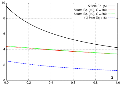
Figure 5: Entropy $S$ and mean sequence length $\langle L\rangle$ in the random model. Entropies for $R=700$ and $R=800$ nearly overlap.

These quantities satisfy the following linear relation in the domain of $a\in[0;\frac{1}{2}]$:

$$\langle L\rangle\simeq 1.549\,S-4.245\qquad\textrm{for}\quad R=700,$$

$$\langle L\rangle\simeq 1.496\,S-4.110\qquad\textrm{for}\quad R=800.$$

It becomes thus clear that the proposed simple model can be used as the principal approximation requiring further adjustments to account for finer effects linked in particular with the exact relative numbers of nucleobases in different mtDNAs.

5 Frequency spectra

From a rank–frequency distribution one can obtain the so called frequency spectrum $N_{j}$, which is the number of items occurring exactly $j$ times [45, 46]. The spectra for nucleotide sequences of species analyzed in the present work are plotted in Fig. 6.

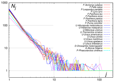
Figure 6: Frequency spectra. The first capital letter before the hyphen serves to distinguish families.

In the domain of low ranks, frequency spectra of words were shown to satisfy the following model inspired by the Bose-distribution [47, 48, 49]:

$$N_{j}=\frac{1}{z^{-1}X\left(\frac{(j-1)^{\gamma}}{T}\right)-1}\qquad\textrm{with\quad$X(t)=e^{t}$}.$$ (24)

The fugacity analog $z$ is fixed by the number of hapax legomena (items occurring only once in a given sample) $N_{1}$:

$$z=\frac{N_{1}}{N_{1}+1}.$$ (25)

The remaining parameters $\gamma$ and $T$ are obtained by fitting Eq. (24) to the observed data.

As frequency spectra corresponding to word distributions typically have thick tails, a modification of the above model with nonadditive statistics was also developed [50, 40]. In particular, one can use $X(t)=\exp_{\kappa}(t)$, where the $\kappa$-exponential [51, 52] is defined as

$$\exp_{\kappa}(x)=\left(\sqrt{1+\kappa^{2}x^{2}}+\kappa x\right)^{\frac{1}{\kappa}}$$ (26)

reducing to the ordinary exponential in the limit of $\kappa\to 0$.

We have applied this approach to nucleotide sequences. Some results of fitting are demonstrated in Fig. 7.

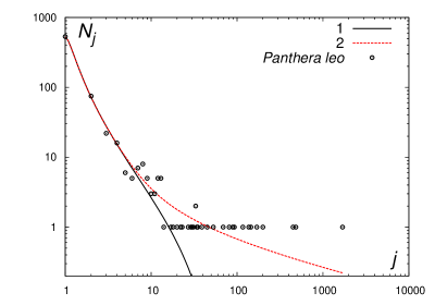
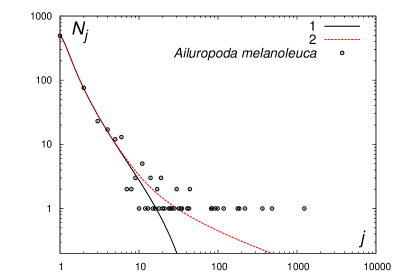
Figure 7: Fitting frequency spectra corresponding to mitochondrial genomes of lion (top panel) and giant panda (bottom panel). Fits with ordinary exponentials are solid lines (1) and fits using $\kappa$-exponentials are dashed lines (2).

Figure 8 summarizes the obtained values of parameters for all the species studied in the present work. Eq. (24) with ordinary exponential was fitted to the observed data via two parameters, $\gamma$ and $T$, while the fitting with $\kappa$-exponential was made via $\kappa$ and $T$ at fixed $\gamma=1.5$.

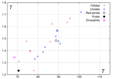
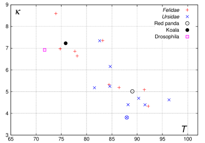
Figure 8: Values of $T$–$\gamma$ (top panel) and $T$–$\varkappa$ (bottom panel) for families and species analyzed in the present work.

The grouping of different species within families with respect to $\gamma$, $\kappa$, and $T$ parameters is much weaker comparing to the parameters analyzed in Sec. 3, so the former set can be used only as a supplementary discrimination tool.

Still, as we can observe from Fig. 8, cats (Felidae) generally have longer tails comparing to bears (Ursidae; mean value $\langle\kappa\rangle_{\rm F}=6.3$ versus $\langle\kappa\rangle_{\rm U}=5.1$) but lower “temperatures” ($\langle T\rangle_{\rm F}=82$ versus $\langle T\rangle_{\rm U}=87$).

6 Conclusions

An approach was proposed for the analysis of nucleotide sequences in mitochondrial DNA in order to find a set of parameters discriminating taxonomic ranks in the biological classification like families and possibly genera. The approach was tested on two carnivoran families, Felidae (cats) and Ursidae (bears).

The nucleotide sequences were defined using the linguistic analogy, with the most frequent nucleobase (adenine in all the analyzed cases) as a separating element (a whitespace analog separating nucleotide “words”). The rank–frequency distributions were compiled, entropy $S$ and mean length $\langle L\rangle$ were calculated. The latter pair of parameters was shown to serve well for the discrimination of cat and bear families. As one of the results, we were able to confirm that Ailuropoda melanoleuca (giant panda) is a bear, that A. melanoleuca and Ailurus fulgens (red panda) belong to different families, and that Phascolarctos cinereus (koala) is not a bear at all.

A linear relation was observed between entropy $S$ and mean length $\langle L\rangle$, which triggered a search for a simplified model describing these parameters. Such a model yielding nearly linear relation for $S$ and $\langle L\rangle$ in the appropriate range of values was found. Further adjustments are required in order to achieve not only a qualitative but also a quantitative agreement with the observed data.

The so called frequency spectra obtained from the rank–frequency distributions were modeled using a nonadditive modification of the Bose-distribution. Such an approach allowed for better description of thick (or long) tails in the spectra. Various parameters describing families and species were obtained. Unlike entropy and mean sequence length, they cannot serve for a decisive separation of animal families. Still, it was found that on average the frequency spectra of Felidae (cats) have longer tails than those of the Urdidae (bears) family.

In summary, the proposed approaches can be used in studies of mitochondrial genomes as the suggested set of parameters serve to discriminate animal families. Inclusion of other species is planned in future in order to check the applicability of the approaches and to define the ranges of parameters corresponding to families and genera.

References

- [1] Liudmila Rozanova and Marián Boguñá. Dynamical properties of the herding voter model with and without noise. Phys. Rev. E, 96:012310, 2017.
- [2] William Pickering and Chjan Lim. Solution to urn models of pairwise interaction with application to social, physical, and biological sciences. Phys. Rev. E, 96:012311, 2017.
- [3] James Burridge. Spatial evolution of human dialects. Phys. Rev. X, 7:031008, 2017.
- [4] Dorota Lipowska and Adam Lipowski. Language competition in a population of migrating agents. Phys. Rev. E, 95:052308, 2017.
- [5] Henri Benisty. Simple wealth distribution model causing inequality-induced crisis without external shocks. Phys. Rev. E, 95:052307, May 2017.
- [6] Bertrand Ottino-Löffler, Jacob G. Scott, and Steven H. Strogatz. Takeover times for a simple model of network infection. Phys. Rev. E, 96:012313, 2017.
- [7] Daniele De Martino, Fabrizio Capuani, and Andrea De Martino. Quantifying the entropic cost of cellular growth control. Phys. Rev. E, 96:010401, 2017.
- [8] Chikara Furusawa and Kunihiko Kaneko. Zipf’s law in gene expression. Phys. Rev. Lett., 90:088102, 2003.
- [9] Dirson Jian Li and Shengli Zhang. Reconfirmation of the three-domain classification of life by cluster analysis of protein length distributions. Mod. Phys. Lett. B, 23(29):3471–3489, 2009.
- [10] Nathan Harmston, Wendy Filsell, and Michael P. H. Stumpf. What the papers say: Text mining for genomics and systems biology. Human Genomics, 5(1):17–29, 2010.
- [11] S. Eroglu. Language-like behavior of protein length distribution in proteomes. Complexity, 20(2):12–21, 2014.
- [12] Sertac Eroglu. Self-organization of genic and intergenic sequence lengths in genomes: Statistical properties and linguistic coherence. Complexity, 21(1):268–282, 2015.
- [13] Bruce Alberts, Alexander Johnson, Julian Lewis, Martin Raff, Keith Roberts, and Peter Walter. Molecular biology of the cell. Garland Science, New York, NY, sixth edition, 2015.
- [14] J.-W. Taanman. The mitochondrial genome: structure, transcription, translation and replication. Biochimica et Biophysica Acta, 1410(2):103–123, 1999.
- [15] David R. Wolstenholme. Animal mitochondrial DNA: Structure and evolution. International Review of Cytology, 141:173–216, 1992.
- [16] J. B. Estoup. Gammes sténographiques : méthode & exercices pour l’acquisition de la vitesse. Institut Sténographique de France, Paris, 4e édition, 1916.
- [17] E. U. Condon. Statistics of vocabulary. Science, 67(1733):300, 1928.
- [18] George Kingsley Zipf. The Psychobiology of Language. Houghton Mifflin, New York, 1935.
- [19] G. K. Zipf. Human Behavior and the Principle of Least Effort. Addison-Wesley, Cambridge, MA, 1949.
- [20] R. Ferrer i Cancho and R. V. Solé. Two regimes in the frequency of words and the origins of complex lexicons: Zipf’s law revisited. Journal of Quantitative Linguistics, 8(3):165–173, 2001.
- [21] M. A. Montemurro. Beyond the Zipf–Mandelbrot law in quantitative linguistics. Physica A, 300:567–578, 2001.
- [22] Le Quan Ha, E. I. Sicilia-Garcia, Ji Ming, and F. J. Smith. Extension of Zipf’s law to words and phrases. In Proceedings of the 19th International Conference on Computational Linguistics, COLING ’02, pages 315–320, Stroudsburg, PA, USA, 2002. Association for Computational Linguistics.
- [23] Steven T. Piantadosi. Zipf’s word frequency law in natural language: A critical review and future directions. Psychonomic Bulletin & Review, 21(5):1112 1130, 2014.
- [24] Jake Ryland Williams, Paul R. Lessard, Suma Desu, Eric M. Clark, James P. Bagrow, Christopher M. Danforth, and Peter Sheridan Dodds. Zipf’s law holds for phrases, not words. Scientific Reports, 5:12209:1–7, 2015.
- [25] Martin Gerlach, Francesc Font-Clos, and Eduardo G. Altmann. Similarity of symbol frequency distributions with heavy tails. Phys. Rev. X, 6:021009, 2016.
- [26] Yurij Holovatch, Ralph Kenna, and Stefan Thurner. Complex systems: physics beyond physics. European Journal of Physics, 38(2):023002, 2017.
- [27] A. Ghosh, A. Chatterjee, A. S. Chakrabarti, and B. K. Chakrabarti. Zipf’s law in city size from a resource utilization model. Phys. Rev. E, 90(4):042815, 2014.
- [28] Elsa Arcaute, Erez Hatna, Peter Ferguson, Hyejin Youn, Anders Johansson, and Michael Batty. Constructing cities, deconstructing scaling laws. Journal of The Royal Society Interface, 12(102), 2014.
- [29] Bin Jiang, Junjun Yin, and Qingling Liu. Zipf’s law for all the natural cities around the world. International Journal of Geographical Information Science, 29(3):498–522, 2015.
- [30] Shuhei Aoki and Makoto Nirei. Zipf’s law, Pareto’s law, and the evolution of top incomes in the United States. American Economic Journal: Macroeconomics, 9(3):36–71, 2017.
- [31] O. Ogasawara, Sh. Kawamoto, and K. Okubo. Zipf’s law and human transcriptomes: an explanation with an evolutionary model. Comptes Rendus Biologies, 326:1097–1101, 2003.
- [32] Michael Sheinman, Anna Ramisch, Florian Massip, and Peter F. Arndt. Evolutionary dynamics of selfish DNA explains the abundance distribution of genomic subsequences. Sci. Rep., 6:30851, 2016.
- [33] Damián H. Zanette. Zipf’s law and the creation of musical context. Musicae Scientiae, 10(1):3–18, 2006.
- [34] Laurence Aitchison, Nicola Corradi, and Peter E. Latham. Zipf’s law arises naturally when there are underlying, unobserved variables. PLoS Computational Biology, 12(12):e1005110:1–32, 2016.
- [35] Stephen J. O’Brien, Warren Johnson, Carlos Driscoll, Joan Pontius, Jill Pecon-Slattery, and Marilyn Menotti-Raymond. State of cat genomics. Trends in Genetics, 24(6):268–279, 2008.
- [36] Li Yu, Yi-Wei Li, Ryder Oliver A., and Zhang Ya-Ping. Analysis of complete mitochondrial genome sequences increases phylogenetic resolution of bears (Ursidae), a mammalian family that experienced rapid speciation. BMC Evolutionary Biology, 7:198, 2007.
- [37] The National Center for Biotechnology Information, https://www.ncbi.nlm.nih.gov.
- [38] David B. Searls. The linguistics of DNA. American Scientist, 80(6):579–591, 1992.
- [39] Sungchul Ji. The linguistics of DNA: Words, sentences, grammar, phonetics, and semantics. Ann. New York Acad. Sci., 870:411–417, 1999.
- [40] A. Rovenchak and S. Buk. Part-of-speech sequences in literary text: Evidence from Ukrainian. J. Quant. Ling., 25(1):1–21, 2018.
- [41] Gerhard Leitner and Inke Sieloff. Aboriginal words and concepts in Australian English. World Englishes, 17(2):153–169, 1998.
- [42] Theodore Sherman Palmer. Index Generum Mammalium: A list of the genera and families of mammals. North American Fauna, 23:1–984, 1904.
- [43] Madhu Raman Acharya. Nepal concise encyclopedia: a comprehensive dictionary of facts and knowledge about the kingdom of Nepals. Geeta Sharma, Kathmandu, 2043 [1986].
- [44] Angela R. Glatston, editor. Red Panda: Biology and Conservation of the First Panda. Noyes Series in Animal Behavior, Ecology, Conservation, and Management. Elsevier / Academic Press, Amsterdam ; Boston, 2011.
- [45] J. Tuldava. The frequency spectrum of text and vocabulary. J. Quant. Ling., 3(1):38–50, 1996.
- [46] I.-I. Popescu, G. Altmann, P. Grzybek, B. D. Jayaram, R. Köhler, V. Krupa, J. Mačutek, R. Pustet, L. Uhlířová, and M. N. Vidya. Word frequency studies. Mouton de Gruyter, Berlin ; New York, 2009.
- [47] A. Rovenchak and S. Buk. Application of a quantum ensemble model to linguistic analysis. Physica A, 390(7):1326–1331, 2011.
- [48] A. Rovenchak and S. Buk. Defining thermodynamic parameters for texts from word rank-frequency distributions. J. Phys. Stud., 15(1):1005, 2011.
- [49] A. Rovenchak. Trends in language evolution found from the frequency structure of texts mapped against the Bose-distribution. J. Quant. Ling., 21(3):281–294, 2014.
- [50] A. Rovenchak. Models of frequency spectrum in texts based on quantum distributions in fractional space dimensions. In I. Dumitrache, A. M. Florea, F. Pop, and A. Dumitraşcu, editors, 20th International Conference on Control Systems and Computer Science CSCS 2015: Proceedings, 27–29 May 2015, Bucharest, Romania, volume 2, pages 645–649, Los Alamitos, CA, 2015. IEEE Computer Society.
- [51] G. Kaniadakis. Non-linear kinetics underlying generalized statistics. Physica A, 296:405–425, 2001.
- [52] G. Kaniadakis. Theoretical foundations and mathematical formalism of the power-law tailed statistical distributions. Entropy, 15(10):3983–4010, 2013.