Learning Inductive Biases with Simple Neural Networks

Abstract

People use rich prior knowledge about the world in order to efficiently learn new concepts. These priors–also known as “inductive biases”–pertain to the space of internal models considered by a learner, and they help the learner make inferences that go beyond the observed data. A recent study found that deep neural networks optimized for object recognition develop the shape bias citep(Ritter et al., 2017), an inductive bias possessed by children that plays an important role in early word learning. However, these networks use unrealistically large quantities of training data, and the conditions required for these biases to develop are not well understood. Moreover, it is unclear how the learning dynamics of these networks relate to developmental processes in childhood. We investigate the development and influence of the shape bias in neural networks using controlled datasets of abstract patterns and synthetic images, allowing us to systematically vary the quantity and form of the experience provided to the learning algorithms. We find that simple neural networks develop a shape bias after seeing as few as 3 examples of 4 object categories. The development of these biases predicts the onset of vocabulary acceleration in our networks, consistent with the developmental process in children.

Keywords: neural networks; inductive biases; learning-to-learn; word learning

Humans possess the remarkable ability to learn a new concept from seeing just a few examples. A child can learn the meaning of a new word such as “fork” after observing only one or a handful of different forks citep(Bloom, 2000). In contrast, state-of-the-art artificial learning systems use hundreds or thousands of examples per class when learning to recognize the same objects citep(e.g., Krizhevsky et al., 2012; Szegedy et al., 2015). Consequently, significant effort is ongoing to understand what cognitive and neural mechanisms enable efficient concept learning citep(Lake et al., 2017). In this paper, we perform a series of developmentally-informed neural network experiments to study the computational basis of efficient word learning.

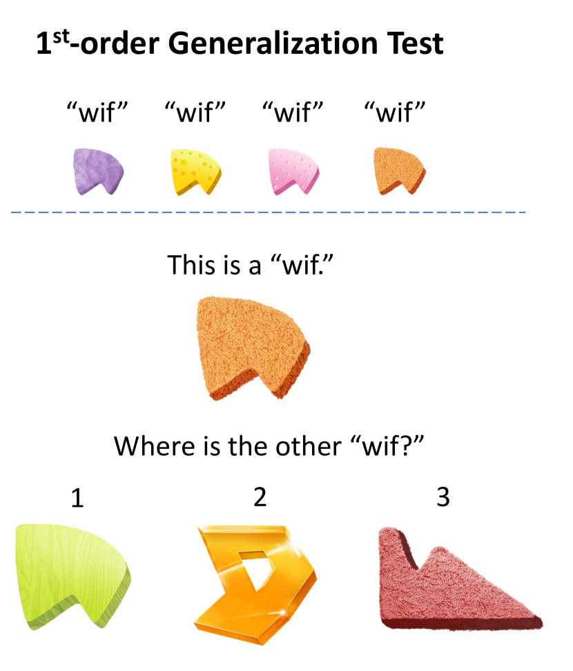
(a)

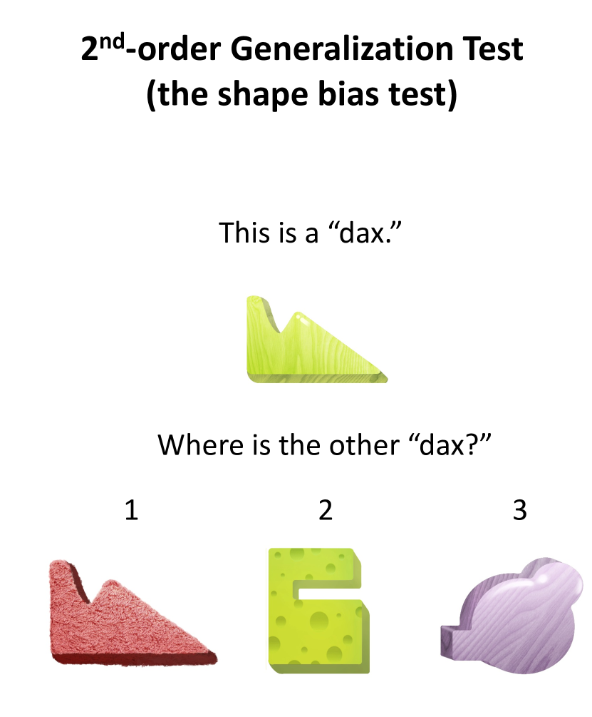
(b)

Figure 1: Shape bias generalization tests. The 1st-order test, shown in (a), assesses if a child has learned to generalize a familiar object name to a novel exemplar according to shape. This is the first step of shape bias development. The 2nd-order test, shown in (b), assesses if the child has learned to generalize a novel name to a novel exemplar by shape, the second and final step of shape bias development.

If a learner extrapolates beyond the data, then another source of information must make up the difference; prior knowledge or “inductive biases” must help constrain the space of models considered by the learner citep(Tenenbaum et al., 2011; Michalski et al., 2013; Lake et al., 2017). For example, children make use of the shape bias–the assumption that objects that have the same name will tend to have the same shape–when learning new object names, and thus they attend to shape more often than color, material and other properties when generalizing a novel name to new examples (Fig. 1(b)) citep(Landau et al., 1988). Similarly, children assume that object names are mutually exclusive, i.e. that a novel name probably refers to a novel object rather than a familiar object citep(Markman & Wachtel, 1988). Although the origin of inductive biases is not always clear, results show that children, adults and primates can “learn-to-learn” or form higher-order generalizations that improve the efficiency of future learning citep(Harlow, 1949; Smith et al., 2002; Dewar & Xu, 2010).

Researchers have proposed a number of computational models to explain how inductive biases are acquired and harnessed for future learning. Hierarchical Bayesian Models (HBMs) enable probabilistic inference at multiple levels simultaneously, allowing the model to learn the structure of individual concepts while also learning about the structure of concepts in general citep(Gelman et al., 2013; Kemp et al., 2007; Salakhutdinov et al., 2012). These models have been used to explain various forms of “learning-to-learn,” including learning a shape bias citep(Kemp et al., 2007). However, it is currently difficult to apply HBMs to the type of high-dimensional visual and auditory stimuli that children receive; there have been successes citep(Salakhutdinov et al., 2013; Lake et al., 2015), but neural networks are still the most general solution to learning effectively from many different forms of raw data citep(LeCun et al., 2015). Utilizing this property, here we use neural networks to study learning-to-learn in different settings of varying stimulus complexity, with the goal of isolating the fundamentals of the learning dynamics.

Most related to our work here are studies by citeColunga & Smith (2005) and citeRitter et al. (2017) investigating neural network accounts of shape bias development. citeColunga & Smith (2005) showed that a simple recurrent neural network, trained via Hebbian learning, can acquire a shape bias for solid objects and a material bias for non-solid objects. These simulations demonstrate that neural networks can form different expectations for different kinds of objects, but they raise many new questions regarding the conditions required to develop these types of biases. For example, the authors used highly simplified bit-vector data, and it is unclear whether their findings generalize to more complex or realistic stimuli. Furthermore, the authors did not systematically vary the quantity of experience provided to the networks, and thus we do not know the exact conditions in which biases arise and whether these networks can compete with the strong sample efficiency of HBMs citep(Kemp et al., 2007). In a recent study, citeRitter et al. (2017) found that performance-optimized deep neural networks (DNNs) develop the shape bias when trained on the popular ImageNet object recognition dataset consisting of raw naturalistic images. These results highlight an exciting possible connection between large-scale DNNs and developmental psychology, though many questions still remain. ImageNet–which contains about 1200 labeled examples of 1000 different object categories–is a poor proxy for the experience of a developing child, who typically develops a shape bias with no more than 50-100 object words in her vocabulary citep(Gershkoff-Stowe & Smith, 2004). Whether these networks can acquire the shape bias with more appropriate training sets is unclear. Furthermore, although the development of the shape bias is known to predict the onset of vocabulary acceleration in children citep(Gershkoff-Stowe & Smith, 2004), we do not know whether the same holds for DNNs.

In a related study, citeHill et al. (2017) trained a neural network agent to navigate around a virtual 3D world and collect objects according to name-based language commands. Although the authors draw inspiration from developmental psychology, the agent in this experiment is asked to learn a variety of tasks simultaneously: visual perception, language comprehension and navigation. Further work is necessary to isolate the dynamics of learning-to-learn in neural networks.

We investigate the development and influence of inductive biases in neural networks using artificial object stimuli that allow us to systematically vary the quality and form of the experience provided. Specifically, we use an experimental paradigm from developmental psychology citep(Smith et al., 2002) to train and evaluate the networks. Beginning with simple bit-vector data akin to citeColunga & Smith (2005), we systematically vary the number of categories and the number of examples in the training set, and for each pairing the trained networks are evaluated for two different forms of generalization (Fig. 1) as well as for changes in perceptual sensitivity. Parallel experiments are then performed with raw image data, where each image consists of a 2D object with a particular shape, color and texture. In a final set of experiments, we examine the dynamics of learning-to-learn by analyzing the relationship between shape bias acquisition and the rate of word learning, mirroring an analogous study from developmental psychology citep(Gershkoff-Stowe & Smith, 2004).

Experiments

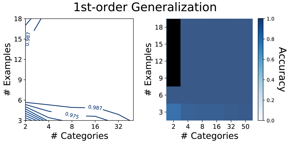
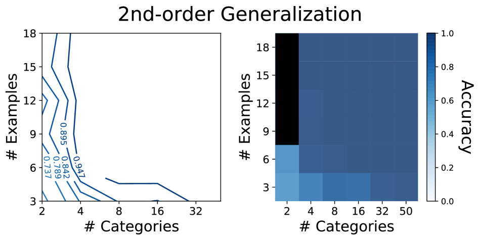
Figure 2: MLP generalization results for explicit shape bias training with various training set sizes. The number of categories and number of examples per category provided to the network are shown on the x and y axes, respectively. Plots show accuracy over 1000 trials of the specified generalization test, averaged from 10 training runs. The same data is shown in both contour and heatmap format. With 2 categories, only 8 unique examples are feasible; thus, N/A results are blacked out.

We set out to train neural networks with a learning paradigm used to guide toddlers to the shape bias citep(Smith et al., 2002). In this paradigm, the learner acquires new object names that are organized exclusively by shape, such that different instances of the same object category are identical in shape but contrast sharply in color and material. This is reflective of the fact that a child’s early noun vocabulary consists predominantly of shape-based categories citep(Samuelson & Smith, 1999), although not with the same purity as the shape bias training. As in previous computational modeling work citep(Kemp et al., 2007; Colunga & Smith, 2005), we focus on purified training with shape-based categories, since it provides a controlled test of the artificial learner’s ability to make higher-order generalizations across varying quantities of training experience.

In citeSmith et al. (2002), 17-month-old children were taught 4 new object names (“wif”, “dax”, etc.) over 7 weeks via weekly play sessions. Objects in the study were 3D formations constructed of various materials; each object contained a specific shape, color and texture (material), and their names were organized strictly by shape. During weekly sessions, children played with each object while an adult announced its name repeatedly. By the end of the study, the children had acquired a shape bias–i.e., they had formed the inductive bias that a novel name should be generalized by shape as opposed to color or texture. A control group of children who did not partake in the play sessions did not form this bias.

We use the training paradigm of citeSmith et al. (2002) to study inductive bias learning in neural networks with artificial object datasets. We first perform our computational experiments with abstract bit-vector stimuli, followed by experiments with raw image data. Each constructed object is assigned a shape, color and texture. We train simple neural networks to label objects with category names based on shape. To understand the necessary conditions for successful inductive bias learning, training is performed with various dataset sizes, varying both the number of categories and the number of examples of each category provided to the network. We evaluate the generalization capabilities of the network for each training set using 2 generalization tests modeled after the 2 tests of citeSmith et al. (2002), depicted in Fig. 1.

1-order generalization test.

For this test, toddlers are first presented with an exemplar object that they have seen during training (“wif” in Fig. 1a). Then, they are presented with 3 test objects that they have not seen: 1 that matches the exemplar in shape (item 1 in Fig. 1a), 1 that matches in color (item 2), and 1 that matches in texture (item 3). For each potential match, the other 2 stimulus attributes are novel. The toddlers are asked to select which of the 3 test objects share the same name as the exemplar. Performance is measured as the fraction of trials in which the child selected the correct object, i.e. the shape match. To simulate this test, we create an evaluation set containing groupings of 4 sample objects: an exemplar, a shape match, a color match, and a texture match. The activations of our network’s hidden layer are obtained in response to each object. We then evaluate the cosine similarity between the activations of the exemplar and each test object to determine which object the network perceives to be most similar. Accuracy is defined as the fraction of groupings for which the correct (shape-similar) object is chosen.

2-order generalization test.

For this test, toddlers are first presented with an exemplar object that has a novel label (e.g., “teema”) as well as a novel shape, color and texture. From there, the trial proceeds similarly to those of the 1-order: a shape match, color match and texture match are presented, and the child must select which test object she believes to share a name with the exemplar. All shapes, colors and textures are novel to the child in this test. We simulate the 2-order test with artificial object stimuli similarly to the 1-order case, again using last hidden layer features to evaluate perceptual similarity.

In all simulations, we record accuracy over 1000 simulated test trials as the performance metric for each generalization.

Experiment 1: Multilayer perceptron trained on synthetic objects

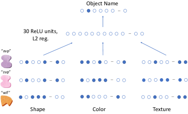
Figure 3: Multilayer perceptron architecture. Shape, color and texture attribute vectors are concatenated and fed to a 30-unit hidden layer, followed by a classification layer. 3 example input objects are shown (only one is presented at a time to the network).

Our first experiment aims to study inductive bias learning in its purest form, using synthetic stimuli with maximal control. Objects are abstract binary patterns, divided into 3 input pools of 20 binary units each (representing the shape, color and texture of the objects; see Fig. 3). We varied the number of categories and number of examples per category in the training set. For datasets with $N$ categories and $K$ examples, we randomly generate $N$ shape patterns, $N$ color patterns, and $N$ texture patterns. For all 3 attributes, each pattern is replicated $K$ times, ensuring equal entropy across the 3. The shape patterns are then aligned with object labels, and the remaining 2 attributes are permuted randomly to create the dataset. A holdout set of shapes, colors and textures is retained for the generalization tests.

We train a multilayer perceptron (MLP) to name objects, as shown in Fig. 3. The network has an input layer of 60 units, a hidden layer of 30 rectified linear units (ReLUs) with L2 regularization, and a softmax output layer to classify the object by name. The softmax layer has $N$ units (1 for each label). We train the network for 200 epochs using negative log-likelihood loss, RMSProp, and batch size min(32, $\frac{N*K}{5}$).

Results.

Initially, as would be expected given the data format, shape is treated the same as other attributes. In the 2-order generalization test, a randomly initialized network selects test objects with the following ratios, on average (50 trials): shape 35%, color 33% and texture 32%. We then trained the network with various dataset sizes. Results for the 1- and 2-order generalizations are shown in Fig. 2, where each setup is an average over 10 networks with different random seeds. We note that acquisition of the 1-order generalization requires less data than that of the 2-order, as predicted by the 2-phase hypothesis citep(Smith et al., 2002). Success in the 1-order test indicates that the network is learning successfully and generalizing to new examples of the training classes. Networks that achieve an accuracy of 0.7 or higher on the 2-order test show a substantial shape bias, and the MLP reaches this threshold at the following points: $N$=2 & $K$=6 (accuracy 0.71) and $N$=4 & $K$=3 (accuracy 0.80). These results reproduce the general pattern of the Hierarchical Bayesian Model (HBM) in citeKemp et al. (2007) and toddlers in citeSmith et al. (2002), who neared the 0.7 shape bias threshold with $N$=4 & $K$=2 (although the toddlers also receive external experience). In contrast, citeColunga & Smith (2005) used $N$=10 & $K$=100 to obtain the shape bias in their networks, using similar abstract patterns. Although HBMs are often noted for their data efficiency, in this case, the neural network was competitive for making 2-order generalizations from limited data.

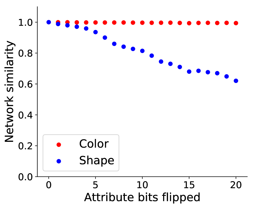
(a) MLP

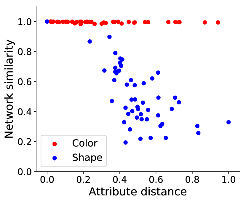
(b) CNN

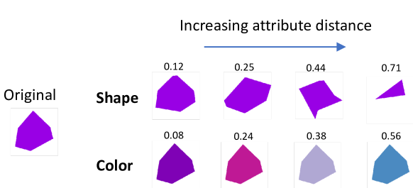
(c) Distance along stimulus dimensions

Figure 4: Perceptual (network) similarity as a function of physical (attribute) distance. A test stimulus is systematically altered along either its shape or color dimension. Network similarity scores are computed between the original stimulus and its altered counterpart.

As another way of demonstrating the learned sensitivity to shape, we perform parametric manipulations of the stimuli. Using an MLP trained with $N$=4 & $K$=6, we probe the shape bias by selecting a novel test stimulus and systematically flipping bits, recording the network similarity between the modified stimulus and the original. For comparison, a similar test is also performed with color. Results are shown in Fig. 4(a) for 1 test stimulus. Clearly, the network is far more sensitive to changes in shape than changes in color.

Experiment 2: Convolutional network trained on synthetic objects

Our first experiment used highly simplified training stimuli for maximal experimental control. One strength of modern neural network architectures is that they can learn effectively from data in raw and complex forms, a fact we take advantage of in developing Experiment 2. Here we ask whether similar learning-to-learn results can be achieved using synthetic object stimuli presented as raw images. This setup presents a more challenging learning problem for the neural network, in terms of making both 1- and 2-order generalizations, since understanding shape requires making abstractions that go substantially beyond separating a pool of input units that directly encode the dimension, as in Experiment 1.

The stimuli are constructed as follows. Each object is a 2D shape of a specified color placed over white background (200x200). Texture is represented in a fourth image channel, independent of RGB space.

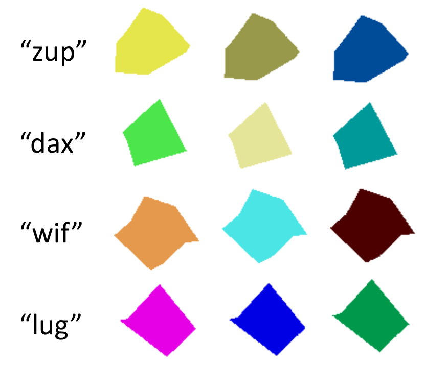
(a)

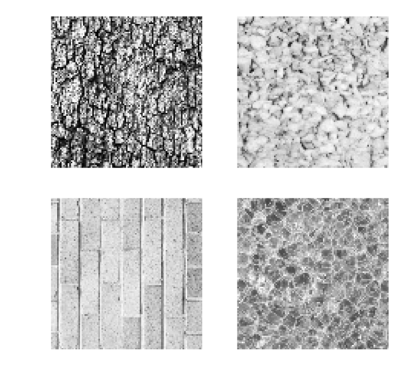
(b)

Figure 5: Training stimuli for Experiment 2. (a) novel objects with various shapes and colors (the first 3 input channels). (b) a few examples of textures that might be found in the 4th input channel.

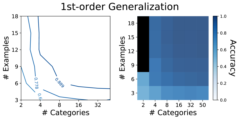
Figure 6: CNN generalization results for various training set sizes. Results show the average of 10 training runs. See Fig. 2 for details.

Examples of our objects are shown in Fig. 5. Object shapes are polygons of random order (uniform 3-10) and randomly sampled vertices, with preference given to points near image boundaries in order to ensure visible-sized objects. Colors are generated to span the RGB vector space with even separation. We use black and white textures from the Brodatz database citep(Brodatz, 1966) for our texture categories. A holdout set of shapes, colors and textures is again retained for testing.

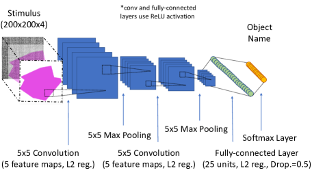
Figure 7: Convolutional network architecture. The network receives 4D image stimuli and is trained to label the object in the image with a category name that is based on shape.

We train a multi-layer convolutional neural network (CNN) citep(LeCun et al., 2015) consisting of two convolution layers with five feature maps, each followed by a max pooling layer. A depiction of this architecture is shown in Fig. 7. The last pooling layer is followed by a fully-connected layer of 25 ReLU units, and the softmax layer again varies in size according to the number of categories. Both the convolutional layers and the fully-connected layer use L2 regularization, the latter also with dropout=0.5. Each object is randomly shifted around image space by a small offset (train and test alike). Training details mimic the MLP, but with 400 epochs.

Results.

The randomly initialized network makes 2-order selections with the following ratios: shape 38%, color 42% and texture 20%. We trained the network using varying dataset sizes, as with our MLP. Results are shown in Fig. 6. Similarly to the MLP, acquisition of the 1-order generalization requires less data than that of the 2-order, supporting the notion that learning the training classes is a simpler task than forming higher-order generalizations. Using the same shape bias threshold of 0.7 2-order score, we find a number of important transition points: $N$=32 & $K$=3 (accuracy 0.74), $N$=8 & $K$=6 (accuracy 0.75), and $N$=4 & $K$=12 (accuracy 0.70). The CNN is thus capable of learning a shape bias from as few as 6 examples of 8 categories, a significant feat given the scale of the input. Notably, the network is able to learn this bias with much less data than citeColunga & Smith (2005) using a data form that is significantly more complex. The CNN of citeRitter et al. (2017) used roughly $N$=1000 & $K$=1200, and developed a shape bias of 0.68 on a shape and color-only task. A key takeaway from our results is that, with concentrated training effort, it is possible to learn this bias from much less data using high-dimensional color images.

As in Experiment 1, we also parametrically manipulated the stimuli to analyze the network’s sensitivity to changes along different stimulus dimensions, finding strong sensitivity to shape but not color (Fig. 4(b) & 4(c); see SM 2 for details). Moreover, in additional experiments, we found that networks trained on color-based categories develop a color bias, and that this bias requires less data than the shape bias (see SM 3 for details).

Experiment 3: The onset of vocabulary acceleration

Our previous experiments confirm that simple neural networks can develop the shape bias from a relatively small number of categories and examples. It remains unclear, however, how the dynamics of bias acquisition relate to the dynamics of word learning. citeGershkoff-Stowe & Smith (2004) showed that the development of the shape bias in toddlers predicts the onset of vocabulary acceleration during early word learning, a phase that begins at ages 16-20 months. Studying 8 children during regular lab sessions at 3-week intervals, the authors found that increasing attention to shape was correlated with increasing rate of vocabulary acquisition in participants. Fig. 8(a) shows the individual growth curves of vocabulary size and shape response for each child. The former variable is measured as the cumulative number of nouns in the child’s vocabulary, and the latter as the cumulative number of times that the child has selected the shape match in a shape bias task akin to the 2-order test. Although the vocabulary curve shows cumulative nouns in whole, the authors also recorded cumulative “count nouns” for each participant, a subset of nouns that is well organized by shape. We focus on the statistics reported for count nouns, as this subset reflects the type of vocabulary that is influenced by the shape bias.

The authors found a few interesting correlations: 1) a correlation between increase in cumulative shape choices and increase in cumulative count nouns across sessions for an individual participant, averaged over participants [average $r=.75$; $p<.05$ for each], and 2) a correlation between average increase in shape choices over the whole experiment and average increase in count nouns, computed across participants [$r=.81$; $p<.05$].

Methods.

Inspired by this study, we train a CNN using our raw image data with the goal of evaluating related correlation metrics for our networks. The participants of citeGershkoff-Stowe & Smith (2004) were not explicitly trained for the shape bias like those of citeSmith et al. (2002); they received natural experience in a home setting, which may have included some words organized by attributes other than shape. Therefore, we train our CNN to simultaneously label the object’s name, which correlates with shape, as well as its color and texture names. Thus, there are now 3 softmax layers in the CNN from Fig. 7, each of which branches independently from the fully-connected layer (see SM 4 for network details). The number of categories along each label dimension and the loss weight assigned to that dimension are determined according to the natural statistics of the early human lexicon citep(Samuelson & Smith, 1999). The chosen ratios are as follows: 60-20-20 shape-color-texture names (36, 12 and 12 categories, respectively). 10 examples of each shape are used, and colors and textures are assigned at random to each stimuli from their 12 categories. We keep a cumulative count of the number of count nouns in the network’s vocabulary, defined as the number of shape categories for which the network has achieved 80% or greater accuracy on the training set. We also keep a cumulative count of shape choices the network makes in a 500-trial 2-order test. This process is repeated with 20 networks, using a different random seed for each network.

Results.

We inspect the “early” word learning period for our networks, defined as the period in which the average vocabulary size across the 20 networks is less than or equal to $2/3$ the total number of count nouns. Beyond this period, which we find to include the first 30 training epochs, the network’s learning begins to flatten. We divide this period into 10 “sessions,” evenly spaced by 3 epochs. The learning curves of our networks are shown in Fig. 8(b). We compute correlation metrics for our networks that are analogous to those of the child study. Looking at increases across the sessions of a single network (metric 1), we find an average correlation of $r=.53$ between increase in cumulative shape choices and increase in cumulative count nouns [$p<.05$ for each]. Further, looking at average increases across the entire 10-session period for each network (metric 2), we find a correlation of $r=0.76$ [$p<.001$] across the 20 networks.

These analyses confirm that the dynamics of shape bias acquisition and early word learning show a considerable dependency on one another in our CNNs, a phenomenon that is mirrored in the early word learning of human children.

Conclusion

Using a set of controlled synthetic experiments, our work provides novel insights about the environmental conditions that enable learning-to-learn in neural networks. Building on the work of citeColunga & Smith (2005) and citeRitter et al. (2017), Experiment 1 showed that simple neural networks can learn a shape bias from stimuli presented as abstract bit patterns with as few as 3 examples of 4 categories. Experiment 2 showed that simple convolutional neural net architectures trained on high-dimensional images can learn a shape bias with as few as 6 examples of 8 object categories. Although Hierarchical Bayesian Models (HBMs) are often noted for their data efficiency, our results indicate that neural networks can approach both HBMs citep(Kemp et al., 2007) and children citep(Smith et al., 2002) in the amount of data required to develop a shape bias. Moreover, we show that the complexity of the data (e.g., binary patterns vs. synthetic images) influences the dynamics of learning, and that neural networks are a powerful tool for understanding these types of interactions.

The development of the shape bias in children is known to correlate with accelerated word learning citep(Gershkoff-Stowe & Smith, 2004), a phenomenon that Experiment 3 confirmed can be mirrored in neural networks. One implication of this finding is that it may be possible to train large-scale image recognition models more efficiently after initializing these models with shape bias training. In future work, we hope to investigate this hypothesis with ImageNet-scale DNNs, using an initialization framework designed with the intuitions garnered here.

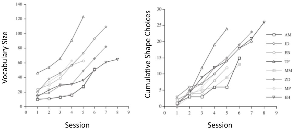
(a) Children

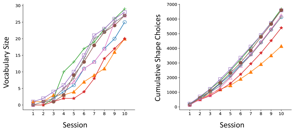
(b) CNN

Figure 8: Learning curves for shape bias and vocabulary. (a) shows the learning curves of the 8 children participants from citeGershkoff-Stowe & Smith (2004). Participants were studied over the course of 5-8 lab sessions. Curves are shown for vocabulary size (left) and cumulative shape choices (right). Here, vocabulary includes all noun types. (b) shows analogous plots for our CNNs. 8 networks are shown, randomly sampled from the total 20 for the sake of visibility. Here, vocabulary is measured only for shape-based object names.

SUPPLEMENTAL MATERIAL

SM 1: Selection of network architectures and training parameters

Architecture.

The MLP architecture for Experiment 1 was chosen ad-hoc before running any experiments. The network receives a 60-dimensional input, and thus, we chose a hidden layer size of 30 units to reduce this dimensionality by a factor of 2. L2 regularization was critical to the performance of the network when small training sets were provided. For Experiment 2, we chose the minimal CNN architecture that could effectively learn the image classification task that it was assigned. We generated a large dataset of 30 categories and 20+ examples per category. Then, we started with a large CNN and iteratively reduced the number of parameters until the minimal architecture was found. L2 regularization was again critical to model performance.

Training parameters.

For both the MLP and the CNN, we train the network to minimize negative log-likelihood loss, using stochastic gradient descent (SGD) with the RMSprop update rule and a typical batch size of 32. There are a few exceptions to this batch size: when the training set is very small, we adjust the batch size to ensure there are at least 5 training batches. Thus, for a training set with $N$ categories and $K$ examples per category (a total of $N*K$ training points), we use a batch size of min(32, $\frac{N*K}{5}$). The number of training epochs was chosen such that the network loss reaches an asymptote for each the MLP and CNN. Training loss is monitored and used to save the best model.

SM 2: Experiment 2 perceptual sensitivity tests

As in Experiment 1, for Experiment 2 we parametrically manipulate the stimuli to analyze the network’s sensitivity to changes along different stimulus dimensions, using a CNN trained with $N$=30 & $K$=10. Distance in shape space is quantified as the Modified Hausdorff Distance citep(Dubuisson & Jain, 1994) between the shape pair. In color space, physical distance is quantified using the cosine similarity of the RGB vector pair. Beginning with an exemplar object stimuli, we sample 50 secondary shapes and order them by their distance from the exemplar. We then modify the shape of the exemplar parametrically by stepping along this list, recording network similarities between the original and modified versions in each case. A mirroring experiment is then performed with color; in each case, only 1 attribute is altered at a time. Results are shown in Fig. 4. As with the MLP, our CNN’s selection preferences show a clear parametric dependency on shape, and a much weaker dependency on color

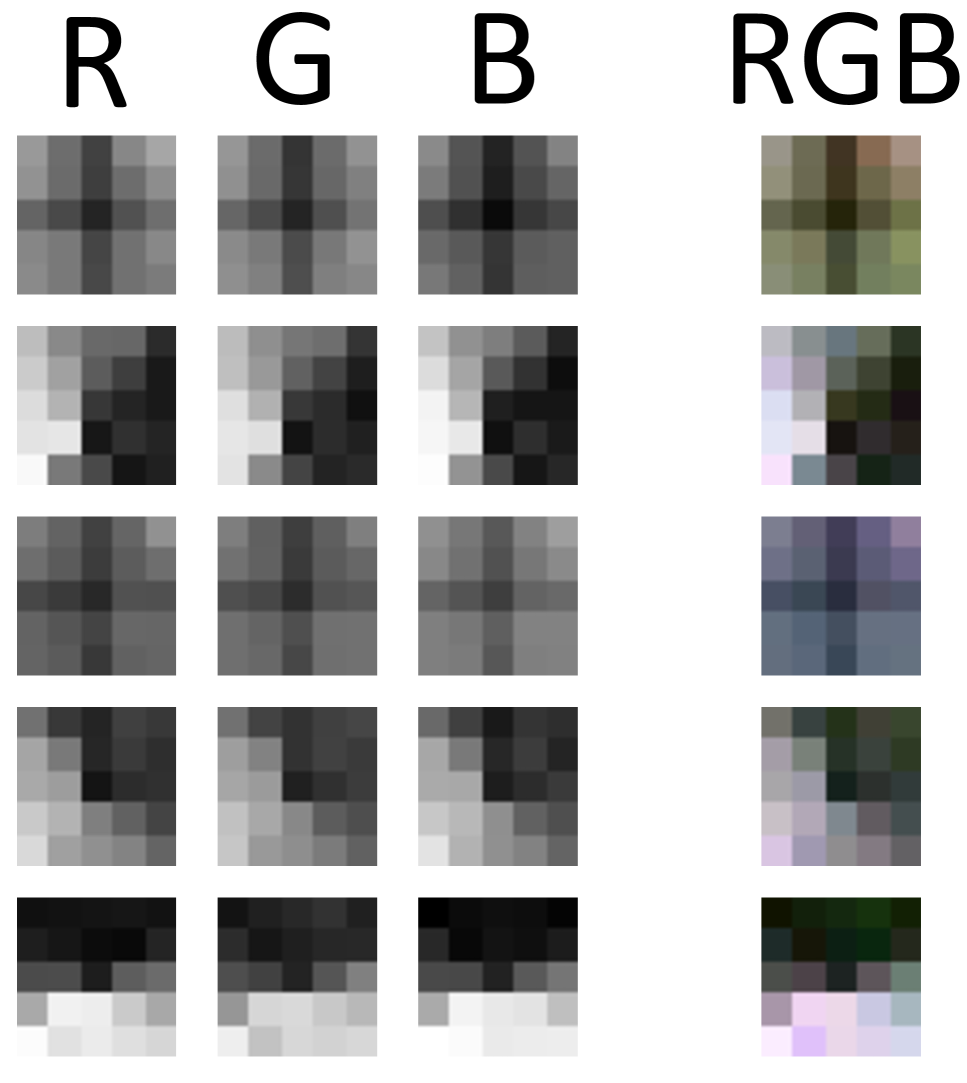
(a) Shape

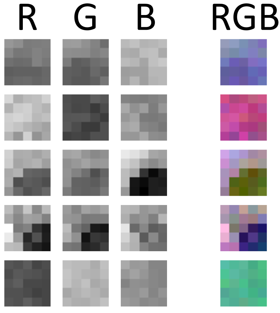
(b) Color

Figure 9: Visualizing RGB channels of learned first-layer convolution filters. (a) shows the filters of our CNN trained with explicit shape bias training ($N$=50 & $K$=18). Each row corresponds to 1 of the 5 filters. The first 3 channels are shown in the ’R’, ’G’ and ’B’ columns, respectively. These 3 channels are shown together in a 4th column, labeled ’RGB’. (b) shows mirroring filters for our CNN trained to label objects with category names based on color. In both (a) and (b), only channels 1-3 of the 4 are shown.

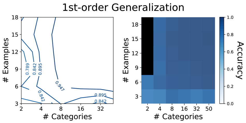
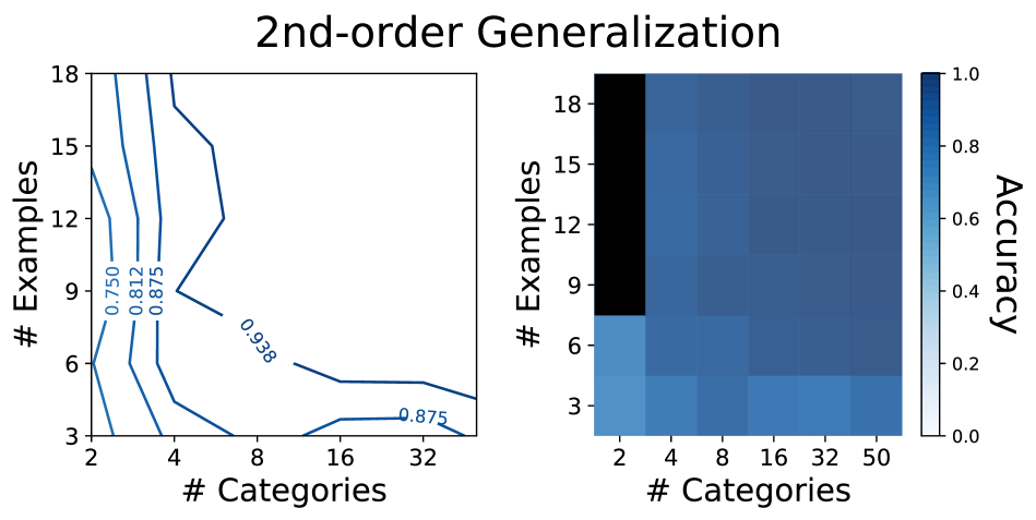
Figure 10: CNN generalization results for color bias training. The network is trained to label objects with category names based on color. In this case, the generalization tests evaluate the fraction of times that the color match is selected. Results in each grid show the average of 10 training runs.

SM 3: Experiment 2 color bias training

For the sake of comparison, in Experiment 2 we also trained our CNN to label objects with names organized by color. Our goal was to compare the required sample complexity for color bias training with that of shape bias training, and to evaluate whether color bias development follows a similar 2-step process. All dataset parameters mirrored those of shape training, except that the object labels were aligned with the color attribute of each training image. Performance on the generalization tests was measured as the fraction of trials for which the network selects the color match. Results for CNN color bias training are shown in Fig. 10. Notably, the color-trained CNN requires a smaller sample complexity to achieve 0.7 accuracy on the 2-order test, reaching a score of 0.73 with $N$=2 & $K$=3. Furthermore, this network does not appear to follow the 2-step process of bias development; results for 1- and 2-order generalizations look near-identical to one another. In order to identify a stimulus as a member of a particular color category, the network needs only to find a single pixel of that color, a task that is much simpler than representing and identifying shape. Representing color requires a simple 3D space. By learning to isolate and preserve this space in the hidden layers, the network can easily generalize to novel colors, hence the early 2-order results. We inspected the learned representations of both a shape-trained and a color-trained CNN, trained with $N$=50 & $K$=18, by visualizing the first-layer convolution filters of each network (Fig. 9). As we would expect, filters of the shape-trained CNN look identical across R, G and B channels, as this network needs no sensitivity to color. In contrast, filters of the color-trained CNN vary across channels, indicating that the network has learned a selectivity for color.

SM 4: Experiment 3 network details

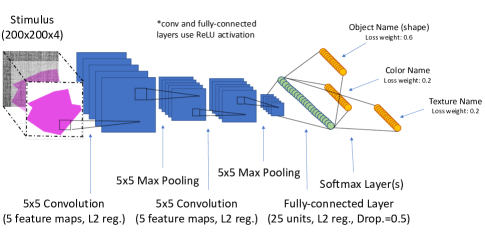
Figure 11: CNN architecture for Experiment 3. The architecture mimics the original CNN of Experiment 2, with the exception of the softmax layer. Here, there are 3 softmax layers (1 for each shape, color and texture), each of which extends from the fully-connected layer.

In Experiment 3, we use a slightly modified version of the CNN from Experiment 2 (see Fig. 11). We train our CNN to simultaneously label the object’s name, which correlates with shape, as well as its color and texture names. The CNN thus has 3 softmax layers, each of which extends from the same fully-connected layer, and each of which has its own negative log-likelihood loss function. The training loss is computed as a weighted average of the 3 losses, with weights of 0.6, 0.2 and 0.2 assigned to shape, color and texture, respectively:

$$Loss=\\ 0.6*shape\_loss+0.2*color\_loss+0.2*texture\_loss$$

References

- Bloom (2000) Bloom, P. (2000). How children learn the meanings of words. Cambridge, MA: MIT Press.
- Brodatz (1966) Brodatz, P. (1966). Textures: a photographic album for artists and designers. New York, NY: Dover Publications.
- Colunga & Smith (2005) Colunga, E., & Smith, L. B. (2005). From the lexicon to expectations about kinds: a role for associative learning. Psychol. Rev., 112(2), 347–382.
- Dewar & Xu (2010) Dewar, K. M., & Xu, F. (2010). Induction, overhypothesis, and the origin of abstract knowledge: evidence from 9-month-old infants. Psychol. Sci., 21(12), 1871–1877.
- Dubuisson & Jain (1994) Dubuisson, M., & Jain, A. K. (1994). A modified hausdorff distance for object matching. In 12th icpr (pp. 566–568).
- Gelman et al. (2013) Gelman, A., Carlin, J., Stern, H., Dunson, D., Vehtari, A., & Rubin, D. (2013). Bayesian data analysis. Boca Raton, FL: CRC.
- Gershkoff-Stowe & Smith (2004) Gershkoff-Stowe, L., & Smith, L. B. (2004). Shape and the first hundred nouns. Child Dev., 75(4), 1098–1114.
- Harlow (1949) Harlow, H. F. (1949). The formation of learning sets. Psychol. Rev., 56(1), 51–65.
- Hill et al. (2017) Hill, F., Hermann, K. M., Blunsom, P., & Clark, S. (2017). Grounded language learning in a 3d simulated world. arXiv:1710.09867.
- Kemp et al. (2007) Kemp, C., Perfors, A., & Tenenbaum, J. B. (2007). Learning overhypotheses with hierarchical bayesian models. Dev. Sci., 10(3), 307–321.
- Krizhevsky et al. (2012) Krizhevsky, A., Sutskever, I., & Hinton, G. (2012). Imagenet classification with deep convolutional neural networks. In 25th nips (pp. 1097–1105).
- Lake et al. (2015) Lake, B. M., Salakhutdinov, R., & Tenenbaum, J. B. (2015). Human-level concept learning through probabilistic program induction. Science, 350(6266), 1332–1338.
- Lake et al. (2017) Lake, B. M., Ullman, T. D., Tenenbaum, J. B., & Gershman, S. J. (2017). Building machines that learn and think like people. Behav. Brain Sci., 40.
- Landau et al. (1988) Landau, B., Smith, L. B., & Jones, S. S. (1988). The importance of shape in early lexical learning. Cog. Dev., 3(3), 299–321.
- LeCun et al. (2015) LeCun, Y., Bengio, Y., & Hinton, G. (2015). Deep learning. Nature, 521(7553), 436–444.
- Markman & Wachtel (1988) Markman, E. M., & Wachtel, G. F. (1988). Children’s use of mutual exclusivity to constrain the meaning of words. Cog. Psychol., 20(2), 121–157.
- Michalski et al. (2013) Michalski, R. S., Carbonell, J. G., & Mitchell, T. M. (2013). Machine learning: an artificial intelligence approach. Berlin: Springer Science+Business Media.
- Ritter et al. (2017) Ritter, S., Barrett, D. G. T., Santoro, A., & Botvinick, M. M. (2017). Cognitive psychology for deep neural networks: a shape bias case study. In 34th icml (pp. 2940–2949).
- Salakhutdinov et al. (2012) Salakhutdinov, R., Tenenbaum, J., & Torralba, A. (2012). One-shot learning with a hierarchical nonparametric bayesian model. JMLR, 27, 195–207.
- Salakhutdinov et al. (2013) Salakhutdinov, R., Tenenbaum, J. B., & Torralba, A. (2013). Learning with hierarchical-deep models. IEEE Transactions on Pattern Analysis and Machine Intelligence, 35(8), 1958–1971.
- Samuelson & Smith (1999) Samuelson, L. K., & Smith, L. B. (1999). Early noun vocabularies: do ontology, category structure and syntax correspond? Cognition, 73(1), 1–33.
- Smith et al. (2002) Smith, L. B., Jones, S. S., Landau, B., Gershkoff-Stowe, L., & Samuelson, L. (2002). Object name learning provides on-the-job training for attention. Psych. Sci., 13(1), 13–19.
- Szegedy et al. (2015) Szegedy, C., Liu, W., Jia, Y., Sermanet, P., Reed, S., Anguelov, D., … Rabinovich, A. (2015). Going deeper with convolutions. In 2015 cvpr (pp. 1–9).
- Tenenbaum et al. (2011) Tenenbaum, J. B., Kemp, C., Griffiths, T. L., & Goodman, N. D. (2011). How to grow a mind: statistics, structure, and abstraction. Science, 331(6022), 1279–1285.