Statistical tests for extreme precipitation volumes

Abstract. The approaches, based on the negative binomial model for the distribution of duration of the wet periods measured in days, are proposed to the definition of extreme precipitation. This model demonstrates excellent fit with real data and provides a theoretical base for the determination of asymptotic approximations to the distributions of the maximum daily precipitation volume within a wet period as well as the total precipitation volume over a wet period. The first approach to the definition (and determination) of extreme precipitation is based on the tempered Snedecor–Fisher distribution of the maximum daily precipitation. According to this approach, a daily precipitation volume is considered to be extreme, if it exceeds a certain (pre-defined) quantile of the tempered Snedecor–Fisher distribution. The second approach is based on that the total precipitation volume for a wet period has the gamma distribution. Hence, the hypothesis that the total precipitation volume during a certain wet period is extremely large can be formulated as the homogeneity hypothesis of a sample from the gamma distribution. Two equivalent tests are proposed for testing this hypothesis. Both of these tests deal with the relative contribution of the total precipitation volume for a wet period to the considered set (sample) of successive wet periods. Within the second approach it is possible to introduce the notions of relatively and absolutely extreme precipitation volumes. The results of the application of these tests to real data are presented yielding the conclusion that the intensity of wet periods with extreme large precipitation volume increases.

Key words: wet periods, total precipitation volume, negative binomial distribution, asymptotic approximation, extreme order statistic, random sample size, gamma distribution, Beta distribution, Snedecor–Fisher distribution, testing statistical hypotheses.

1 Introduction

Estimates of regularities and trends in heavy and extreme daily precipitation are important for understanding climate variability and change at relatively small or medium time horizons [13]. However, such estimates are much more uncertain compared to those derived for mean precipitation or total precipitation during a wet period [17]. This uncertainty is due to that, first, estimates of heavy precipitation depend closely on the accuracy of the daily records; they are more sensitive to missing values [14, 15]. Second, uncertainties in the estimates of heavy and extreme precipitation are caused by the inadequacy of the mathematical models used for the corresponding calculations. Third, these uncertainties are boosted by the lack of reasonable means for the unambiguous (algorithmic) determination of extreme or anomalouslyly heavy precipitation amplified by some statistical significance problems owing to the low occurrence of such events. As a consequence, continental-scale estimates of the variability and trends in heavy precipitation based on daily precipitation might generally agree qualitatively but may exhibit significant quantitative differences. In [16] a detailed review of this phenomenon is presented where it is noted that for the European continent, most results hint at a growing intensity of heavy precipitation over the last five decades.

At the same time, the climate variability and trends at relatively large time horizons are of no less importance for long-range business, say, agricultural projects and forecasting of risks of water floods, dry spells and other natural disasters. In the present paper we propose a rather reasonable approach to the unambiguous (algorithmic) determination of extreme or abnormally heavy daily and total precipitation within a wet period.

It is traditionally assumed that the duration of a wet period (the number of subsequent wet days) follows the geometric distribution (for example, see [16]). But the sequence of dry and wet days is not only independent, it is also devoid of the Markov property [3]. Our approach introduces the negative binomial model for the duration of wet periods measured in days. This model demonstrates excellent fiting the numbers of successive wet days with the negative binomial distribution with shape parameter less than one (see [2, Gulev]). It provides a theoretical base for the determination of asymptotic approximations to the distributions of the maximum daily precipitation volume within a wet period and of the total precipitation volume for a wet period. The asymptotic distribution of the maximum daily precipitation volume within a wet period turns out to be a tempered Snedecor–Fisher distribution whereas the total precipitation volume for a wet period turns out to be the gamma distribution. Both approximations appear to be very accurate. These asymptotic approximations are deduced using limit theorems for statistics constructed from samples with random sizes.

In this paper, two approaches are proposed to the definition of anomalously extremal precipitation. The first approach to the definition (and determination) of abnormally heavy daily precipitation is based on the tempered Snedecor–Fisher distribution. The second approach is based on the assumption that the total precipitation volume over a wet period has the gamma distribution. This assumption is theoretically justified by a version of the law of large numbers for sums of a random number of random variables in which the number of summands has the negative binomial distribution and is empirically substantiated by the statistical analysis of real data. Hence, the hypothesis that the total precipitation volume during a certain wet period is anomalously large can be formulated as the homogeneity hypothesis of a sample from the gamma distribution. Two equivalent tests are proposed for testing this hypothesis. One of them is based on the beta distribution whereas the second is based on the Snedecor–Fisher distribution. Both of these tests deal with the relative contribution of the total precipitation volume for a wet period to the considered set (sample) of successive wet periods. Within the second approach it is possible to introduce the notions of relatively abnormal and absolutely anomalous precipitation volumes. The results of the application of these tests to real data are presented yielding the conclusion that the intensity of wet periods with anomalously large precipitation volume increases.

The proposed approaches are to a great extent devoid of the drawbacks mentioned above: first, estimates of total precipitation are weakly affected by the accuracy of the daily records and are less sensitive to missing values. Second, they are based on limit theorems of probability theorems that yield unambiguous asymptotic approximations which are used as adequate mathematical models. Third, these approaches provide unambiguous algorithms for the determination of extreme or anomalously heavy daily or total precipitation that do not involve statistical significance problems owing to the low occurrence of such (relatively rare) events.

Our approaches improve the one proposed in [15], where an estimate of the fractional contribution from the wettest days to the total was developed which is less hampered by the limited number of wet days. For this purpose, in [15] an assumption was enacted (without any theoretical justification) that the statistical regularities in daily precipitation follow the gamma distribution and the parameters of the gamma distribution are estimated from the observations. This assumption made it possible to derive a theoretical distribution of the fractional contribution of any percentage of wet days to the total from the gamma distribution function.

The fitted Pareto model for the daily precipitation volume [4] together with the observation that the duration of a wet period has the negative binomial distribution makes it possible to propose a reasonable model for the distribution of the maximum daily precipitation within a wet period as an asymptotic approximation provided by the limit theorems for extreme order statistics in samples with random size. We will give a strict derivation of such a model having the form of the tempered Snedecor–Fisher distribution (that is, the distribution of a positive power of a random variable with the Snedecor–Fisher distribution) and discuss its properties as well as some methods of statistical estimation of its parameters. This model makes it possible to propose the following approach to the definition (and determination) of an anomalously heavy daily precipitation volume. The grounds for this approach is an obvious observation that if $X_{1},X_{2},\ldots,X_{N}$ is a sample of $N$ positive observations, then with finite (possibly, random) $N$, among $X_{i}$’s there is always an extreme observation, say, $X_{1}$, such that $X_{1}\geqslant X_{i}$, $i=1,2,\ldots,N$. Two cases are possible: (i) $X_{1}$ is a ‘typical’ observation and its extreme character is conditioned by purely stochastic circumstances (there must be an extreme observation within a finite homogeneous sample) and (ii) $X_{1}$ is abnormally large so that it is an ‘outlier’ and its extreme character is due to some exogenous factors. It will be shown that the distribution of $X_{1}$ in the ‘typical’ case (i) is the tempered Snedecor–Fisher distribution. Therefore, if $X_{1}$ exceeds a certain (pre-defined) quantile of the tempered f distribution (say, of the orders 0.99, 0.995 or 0.999), then it is regarded as ‘suspicious’ to be an outlier, that is, to be anomalously large (the quantile orders specified above mean that it is pre-determined that one out of a hundred of maximum daily precipitations, one out of five hundred of maximum daily precipitations, or one out of a thousand of maximum daily precipitations is abnormally large, respectively).

Methodically, this approach is similar to the classical techniques of dealing with extreme observations [1]. The novelty of the proposed method is in a more accurate specification of the distribution of extreme daily precipitation. In applied problems dealing with extreme values there is a common tradition which, possibly, has already become a prejudice, that statistical regularities in the behavior of extreme values necessarily obey one of well-known three types of extreme value distributions. In general, this is certainly so, if the sample size is very large, that is, the time horizon under consideration is very wide. In other words, the models based on the extreme value distributions have asymptotic character. However, in real practice, when the sample size is finite and the extreme values of the process under consideration are studied on the time horizon of a moderate length, the classical extreme value distributions may turn out to be inadequate models. In these situations a more thorough analysis may generate other models which appear to be considerably more adequate. This is exactly the case discussed in the present paper. Here, within the first approach, along with the ‘large’ parameter, the expected sample size, one more ‘small’ parameter is introduced and new models are proposed as asymptotic approximations when the small parameter is infinitesimal. These models prove to be exceptionally accurate and demonstrate excellent fit with the observed data.

To construct another test for distinguishing between the cases (i) and (ii) mentioned above, we also strongly improve the results of [16] by giving theoretical grounds for the correct application of the gamma distribution as the model of statistical regularities of total precipitation volume during a wet period. These grounds are based on the negative binomial model for the distribution of the duration of a wet period. In turn, the adequacy of the negative binomial model has serious empirical and theoretical rationale the details of which are described below. With some caveats the gamma model can be also used for the conditional distribution of daily precipitation volumes. The proof of this result is based on the law of large numbers for random sums in which the number of summands has the negative binomial distribution. Hence, the hypothesis that the total precipitation volume during a certain wet period is anomalously large can be re-formulated as the homogeneity hypothesis of a sample from the gamma distribution. Two equivalent statistics are proposed for testing this hypothesis. The corresponding tests are scale-free and depend only on the easily estimated shape parameter of the negative binomial distribution and the time-scale parameter determining the denominator in the fractional contribution of a wet period under consideration. It is worth noting that within the second approach the test for a total precipitation volume during one wet period to be abnormally large can be applied to the observed time series in a moving mode. For this purpose a window (a set of successive observations) is determined. The observations within a window constitute the sample to be analyzed. Let $m$ be the number of observation in the window (the sample size). As the window moves rightward, each fixed observation falls in exactly $m$ successive windows (from $m$th to $N-m+1$, where $N$ denotes the number of wet periods). A fixed observation may be recognized as anomalously large within each of $m$ windows containing this observation. In this case this observation will be called absolutely abnormally large with respect to a given time horizon (determined by the sample size $m$. Also, a fixed observation may be recognized as anomalously large within at least one of $m$ windows containing this observation. In this case the observation will be called relatively abnormally large with respect to a given time horizon.

The preconditions and backgrounds of all the approaches as well as their peculiarities will also be discussed. The main goals of this study are: (i) to introduce the negative binomial distribution as a model distribution to describe the random duration of a wet period and (ii) to show that this model extends the previously used models and better fits to the real observations. Beside that, this paper proves that the (iii) relation of the unique precipitation volume divided by the total precipitation volume taken over the wet period is given by the Snedecor–Fisher distribution and (iv) may be used as a statistical test to estimate the extreme precipitations. This statement also generalizes the previously obtained results from [15]. Finally, the current paper demonstrates that (v) the proposed schemes perfectly fit to the real data.

The paper is organized as follows. In Section 2 we introduce the test for a daily precipitation volume to be abnormally large. In Section 2.1 an asymptotic approximation is proposed for the distribution of the maximum daily precipitation volume within a wet period. Some analytic properties of the obtained limit distribution are described. Section 2.2 contains the results and discussion of fitting the distribution proposed in Section 2.1 to real data. The results of application of the test for a daily precipitation to be anomalously large based on the tempered Snedecor–Fisher distribution to real daily precipitation data are presented and discussed in Section 2.3. Section 3 deals with the test for a total precipitation volume over a wet period to be abnormally large based on testing the homogeneity hypothesis of a sample from the gamma distribution. Two equivalent statistical tests based on Snedecor–Fisher and beta distributions are introduced in Section 3.1. In Section 3.2 the application of these tests to a time series in a moving mode is discussed and the notions of relatively anomalously large and absolutely abnormally large precipitation are given. The results of application of these tests to real daily precipitation data are presented and discussed in Section 3.3. Section 4 is devoted to the main conclusions of the work.

2 The test for a daily precipitation volume to be anomalously large based on the tempered Snedecor–Fisher distribution

At the beginning of this section we introduce some notation that will be used below. All the r.v.’s under consideration are defined on the same probability space $(\Omega,\,\mathfrak{F},\,{\mathbb{P}})$. The results are expounded in terms of r.v.’s with the corresponding distributions. The symbol $\stackrel{{\scriptstyle d}}{{=}}$ denotes the coincidence of distributions.

Let $G_{r,\lambda}$ be a r.v. having the gamma distribution with shape parameter $r>0$ and scale parameter $\lambda>0$, that is:

$${\mathbb{P}}(G_{r,\lambda}<x)=\int\limits_{0}^{x}\frac{\lambda^{r}}{\Gamma(r)}z^{r-1}e^{-\lambda z}dz,\quad x\geqslant 0,$$

Let $W_{\gamma}$ be a r.v. with the Weibull distribution with the distribution function (d.f.) $\big{[}1-e^{-x^{\gamma}}\big{]}{\bf 1}(x\geqslant 0)$ (${\bf 1}(A)$ is the indicator function of a set $A$). The distribution of the r.v. $|X|$, where $X$ is a r.v. with the standard normal d.f., is a folded normal ($x\geqslant 0$), that is:

$${\mathbf{P}}(|X|<x)=2\Phi(x)-1.$$ (1)

Let $S_{\alpha,1}$ and $S^{\prime}_{\alpha,1}$ ($0<\alpha<1$) be i.i.d. r.v.’s with the same strictly stable distribution [18]. So, the density $v_{\alpha}(x)$ of the r.v. $R_{\alpha}=S_{\alpha,1}/S^{\prime}_{\alpha,1}$ can be represented [9, 12] as follows ($x>0$):

$$v_{\alpha}(x)=\frac{\sin(\pi\alpha)x^{\alpha-1}}{\pi[1+x^{2\alpha}+2x^{\alpha}\cos(\pi\alpha)]}.$$ (2)

2.1 The tempered Snedecor–Fisher distribution as an asymptotic approximation to the maximum daily precipitation volume within a wet period

As it has been demonstrated in [4, 11], the asymptotic probability distribution of extremal daily precipitation within a wet period can be represented as follows (here $r>0$, $\lambda>0$, and $\gamma>0$):

$$F(x;r,\lambda,\gamma)=\bigg{(}\frac{\lambda x^{\gamma}}{1+\lambda x^{\gamma}}\bigg{)}^{r},\ \ \ x\geqslant 0.$$ (3)

Moreover, the theoretical conditions of limit theorems correspond with the real data (in sense of fitting Pareto distribution, see [4]). The function (3) is a scale mixture of the Fréchet (inverse Weibull) distribution. It can be demonstrated [4] for a r.v. $M_{r,\gamma,\lambda}$ with a d.f. $F(x;r,\lambda,\gamma)$ that

$$M_{r,\gamma,\lambda}\stackrel{{\scriptstyle d}}{{=}}\Big{(}\frac{Q_{r,1}}{\lambda r}\Big{)}^{1/\gamma}.$$

That is, the distribution of the r.v. $M_{r,\gamma,\lambda}$ up to a non-random scale factor coincides with that of the positive power of a r.v. with the Snedecor–Fisher distribution. In other words, the distribution function $F(x;r,\lambda,\gamma)$ (3) up to a power transformation of the argument $x$ coincides with the Snedecor–Fisher distribution function. In statistics, distributions with arguments subjected to the power transformation are conventionally called tempered. Therefore, we have serious reason to call the distribution $F(x;r,\lambda,\gamma)$ tempered Snedecor–Fisher distribution. Some properties of the distribution of the r.v. $M_{r,\gamma,\lambda}$ were discussed in [4]. In particular, it was shown that the limit distribution (3) can be represented as a scale mixture of exponential or stable or Weibull or Pareto or folded normal laws ($r\in(0,1]$, $\gamma\in(0,1]$, $\lambda>0$):

$$M_{r,\gamma,\lambda}\stackrel{{\scriptstyle d}}{{=}}\frac{G_{r,\lambda}^{1/\gamma}S_{\gamma,1}}{W_{1}}\stackrel{{\scriptstyle d}}{{=}}\frac{W_{\gamma}}{W^{\prime}_{\gamma}}\cdot\frac{1}{Z_{r,\lambda}^{1/\gamma}}\stackrel{{\scriptstyle d}}{{=}}W_{1}\cdot\frac{R_{\gamma}}{W^{\prime}_{1}Z_{r,\lambda}^{1/\gamma}}\stackrel{{\scriptstyle d}}{{=}}\frac{\Pi R_{\gamma}}{Z_{r,\lambda}^{1/\gamma}}\stackrel{{\scriptstyle d}}{{=}}\frac{|X|\sqrt{2W_{1}}R_{\gamma}}{W^{\prime}_{1}Z_{r,\lambda}^{1/\gamma}},$$

where $W_{\gamma}\stackrel{{\scriptstyle d}}{{=}}W^{\prime}_{\gamma}$, $W_{1}\stackrel{{\scriptstyle d}}{{=}}W^{\prime}_{1}$, the r.v. $R_{\gamma}$ has the density (2), the r.v. $\Pi$ has the Pareto distribution (${\mathbb{P}}(\Pi>x)=(x+1)^{-1}$, $x\geqslant 0$), and in each term the involved r.v$:$s are independent.

It should be mentioned that the same mathematical reasoning can be used for the determination of the asymptotic distribution of the maximum daily precipitation within $m$ wet periods with arbitrary finite $m\in\mathbb{N}$. Indeed, fix arbitrary positive $r_{1},\ldots,r_{m}$ and $p\in(0,1)$. Let $N_{r_{1},p}^{(1)},\ldots,N_{r_{m},p}^{(m)}$ be independent random variables having the negative binomial distributions with parameters $r_{j},\,p$, $j=1,\ldots,m$, respectively. By the consideration of characteristic functions it can be easily verified that

$$N_{r_{1},p}^{(1)}+\ldots+N_{r_{m},p}^{(m)}\stackrel{{\scriptstyle d}}{{=}}N_{r,p},$$ (4)

where $r=r_{1}+\ldots+r_{m}$. If all $r_{j}$ coincide, then $r=mr_{1}$ and in accordance with the results of papers [4, 11] and relation (4), the asymptotic distribution of the maximum daily precipitation within $m$ wet periods has the form ($x\geqslant 0$)

$$F^{(m)}(x;r,\lambda,\gamma)=F(x;mr_{1},\lambda,\gamma)=\bigg{(}\frac{\lambda x^{\gamma}}{1+\lambda x^{\gamma}}\bigg{)}^{mr_{1}}.$$

And if now $m$ infinitely increases and simultaneously $\lambda$ changes as $\lambda=cm$, $c\in(0,\infty)$, then, obviously,

$$\lim_{m\to\infty}F^{(m)}(x;r,\lambda,\gamma)=\lim_{m\to\infty}F(x;mr_{1},cm,\gamma)=\lim_{n\to\infty}\Big{(}1-\frac{1}{1+cmx^{\gamma}}\Big{)}^{mr_{1}}=e^{-\mu x^{-\gamma}}$$

with $\mu=(cr_{1})^{-1}$, that is, the distribution function $F^{(m)}(x;r,\lambda,\gamma)$ of the maximum daily precipitation within $m$ wet periods turns into the classical Fréchet distribution.

2.2 The algorithms of statistical fitting of the tempered Snedecor–Fisher distribution model to real data

Some methods of statistical estimation of the parameters $r$, $\lambda$ and $\gamma$ of the tempered Snedecor–Fisher distribution (3) were described in [4]. In this section the algorithms and corresponding formulas for practical computation are briefly given.

Let $\{X_{i,j}\}$, $i=1,\ldots,m$, $j=1,\ldots,m_{i}$, be the precipitation volumes on the $j$th day of the $i$th wet sequence.

$$X^{*}_{k}=\max\{X_{k,1},\ldots,X_{k,m_{k}}\},\ \ \ k=1,\ldots,m.$$ (5)

Let $X^{*}_{(1)},\ldots,X^{*}_{(m)}$ be order statistics constructed from the sample $X^{*}_{1},\ldots,X^{*}_{m}$, where $X^{*}_{k}=\max\{X_{k,1},\ldots,X_{k,m_{k}}\}$. The unknown parameters $r$, $\lambda$ and $\gamma$ can be found as a solution of a following system of equations (for fixed values $p_{1}$, $p_{2}$ and $p_{3}$, $0<p_{1}<p_{2}<p_{3}<1$):

$$X^{*}_{([mp_{k}])}=\left(\frac{p_{k}^{1/r}}{\lambda-\lambda p_{k}^{1/r}}\right)^{1/\gamma},\quad k=1,2,3$$

(here the symbol $[a]$ denotes the integer part of a number $a$).

Proposition 1

The values of parameters $\gamma$ and $\lambda$ can be estimated as follows:

$$\widetilde{\gamma}=\frac{\frac{1}{r}(\log p_{1}-\log p_{3})+\log(1-p_{3}^{\frac{1}{r}})-\log(1-p_{1}^{\frac{1}{r}})}{\log X^{*}_{([mp_{1}])}-\log X^{*}_{([mp_{3}])}},$$ (6)

$$\widetilde{\lambda}=\frac{p_{2}^{\frac{1}{r}}}{(1-p_{2}^{\frac{1}{r}})(X^{*}_{([mp_{2}])})^{\gamma}}.$$ (7)

Proposition 2

If the value of parameter $r$ is estimated as a corresponding parameter of the negative binomial distribution, least squares estimates of parameters $\gamma$ and $\lambda$ are as follows:

$$\widehat{\gamma}=\frac{(m-1)\sum\limits_{i=1}^{m-1}\log\frac{i^{1/r}}{m^{1/r}-i^{1/r}}\log X^{*}_{(i)}-\sum\limits_{i=1}^{m-1}\log X^{*}_{(i)}\sum\limits_{i=1}^{m-1}\log\frac{i^{1/r}}{m^{1/r}-i^{1/r}}}{(m-1)\sum\limits_{i=1}^{m-1}(\log X^{*}_{(i)})^{2}-(\sum\limits_{i=1}^{m-1}\log X^{*}_{(i)})^{2}},$$ (8)

$$\widehat{\lambda}=\exp\Big{\{}\frac{1}{m-1}\Big{(}\sum\nolimits_{i=1}^{m-1}\log\frac{i^{1/r}}{m^{1/r}-i^{1/r}}-\widehat{\gamma}\sum\nolimits_{i=1}^{m-1}\log X^{*}_{(i)}\Big{)}\Big{\}}.$$ (9)

The numerical results of estimation of the parameters of daily precipitation in Potsdam and Elista from $1950$ to $2009$ using both algorithms are presented in Tables 1 and 2. The first column indicates the censoring threshold: since the tempered Snedecor–Fisher distribution is an asymptotic model which is assumed to be more adequate with small ‘‘success probability’’, the estimates were constructed from differently censored samples which contain only those wet periods whose duration is no less than the specified threshold. The second column contains the correspondingly censored sample size. The third and fourth columns contain the sup-norm discrepancy between the empirical and fitted tempered Snedecor–Fisher distribution for two types of estimators (quantile and least squares) described above. The rest columns contain the corresponding values of the parameters estimated by these two methods. According to Tables 1 and 2, the best accuracy is attained when the censoring threshold equals $3$ days for Elista and $5$–$6$ days for Potsdam. The least squares method (8) and (9) leads to the more accurate estimates. The vivid examples of approximation of the real data with the functions $F(x;r,\gamma,\lambda)$ are presented in [4]). The corresponding numerical methods have been implemented using MATLAB built-in programming language.

Table 1: Potsdam ($r=0.847$)

Minimum	Sample	Discrepancy,	Discrepancy,	$\widetilde{\lambda}$	$\widehat{\lambda}$	$\widetilde{\gamma}$	$\widehat{\gamma}$
duration	size	quantile metod:	LS method:	quantile	LS	quantile	LS
		(6), (7)	(8), (9)	method	method	method	method
$1$	$3323$	$0.09$	$0.092$	$0.169$	$0.211$	$1.177$	$1.29$
$2$	$2066$	$0.045$	$0.065$	$0.0381$	$0.0538$	$1.76$	$1.709$
$3$	$1282$	$0.031$	$0.041$	$0.01$	$0.013$	$2.261$	$2.189$
$4$	$862$	$0.026$	$0.027$	$0.00487$	$0.00454$	$2.449$	$2.523$
$6$	$384$	$0.025$	$0.026$	$0.0016$	$0.0012$	$2.822$	$2.948$
$8$	$163$	$0.04$	$0.045$	$0.0007$	$0.0005$	$3.174$	$3.253$
$10$	$73$	$0.041$	$0.042$	$0.0003$	$0.0003$	$3.389$	$3.352$
$15$	$12$	$0.13$	$0.09$	$0.0014$	$0.0009$	$2.667$	$2.972$

Table 2: Elista ($r=0.876$)

Minimum	Sample	Discrepancy,	Discrepancy,	$\widetilde{\lambda}$	$\widehat{\lambda}$	$\widetilde{\gamma}$	$\widehat{\gamma}$
duration	size	quantile metod:	LS method:	quantile	LS	quantile	LS
		(6), (7)	(8), (9)	method	method	method	method
$1$	$2937$	$0.06$	$0.06$	$0.361$	$0.347$	$1.057$	$1.266$
$2$	$1374$	$0.049$	$0.055$	$0.108$	$0.1$	$1.42$	$1.576$
$3$	$656$	$0.041$	$0.045$	$0.0454$	$0.0377$	$1.706$	$1.898$
$4$	$319$	$0.051$	$0.06$	$0.0231$	$0.0272$	$1.899$	$1.94$
$6$	$77$	$0.07$	$0.075$	$0.0178$	$0.0144$	$2.017$	$2.186$
$7$	$42$	$0.15$	$0.01$	$0.0201$	$0.0206$	$1.974$	$2.184$
$8$	$22$	$0.12$	$0.14$	$0.0143$	$0.0355$	$2.003$	$1.769$
$10$	$10$	$0.17$	$0.16$	$0.0137$	$0.0377$	$2.154$	$1.798$

2.3 The examples of statistical analysis of daily precipitation

The approach to the determination of an anomalously heavy daily precipitation is methodically similar to the classical techniques of dealing with extreme observations [1]. The novelty of the proposed method is in an accurate specification of the mathematical model of the distribution of extreme daily precipitation which turned out to be the tempered Snedecor–Fisher distribution.

The algorithm of determination of an anomalously heavy daily precipitation is as follows. First, the parameters of the distribution function $F(x;r,\lambda,\gamma)$ are estimated from the historical data. Second, a small positive number $\varepsilon$ is fixed. Third, the $(1-\varepsilon)$-quantile $\tau(1-\varepsilon;\,r,\lambda,\gamma)$ of the distribution function $F(x;r,\lambda,\gamma)$ is calculated. If the maximum value, say, $X$ of the daily precipitation volume within some wet period exceeds $\tau(1-\varepsilon;\,r,\lambda,\gamma)$, then $X$ is regarded as ‘suspicious’ to be an outlier, that is, to be anomalously large. It is easy to see that the the probability of the error of the first kind (occurring in the case where a ‘regularly large’ maximum value is erroneously recognized as an anomalously large outlier) for this test is approximately equal to $\varepsilon$.

The application of this test to real data is illustrated by Figs. 1 and 2. On these figures the lower horizontal line corresponds to the threshold equal to the quantile of the fitted tempered Snedecor–Fisher distribution of order $0.9$. The middle and upper lines correspond to the quantiles of orders $0.95$ and $0.99$, respectively.

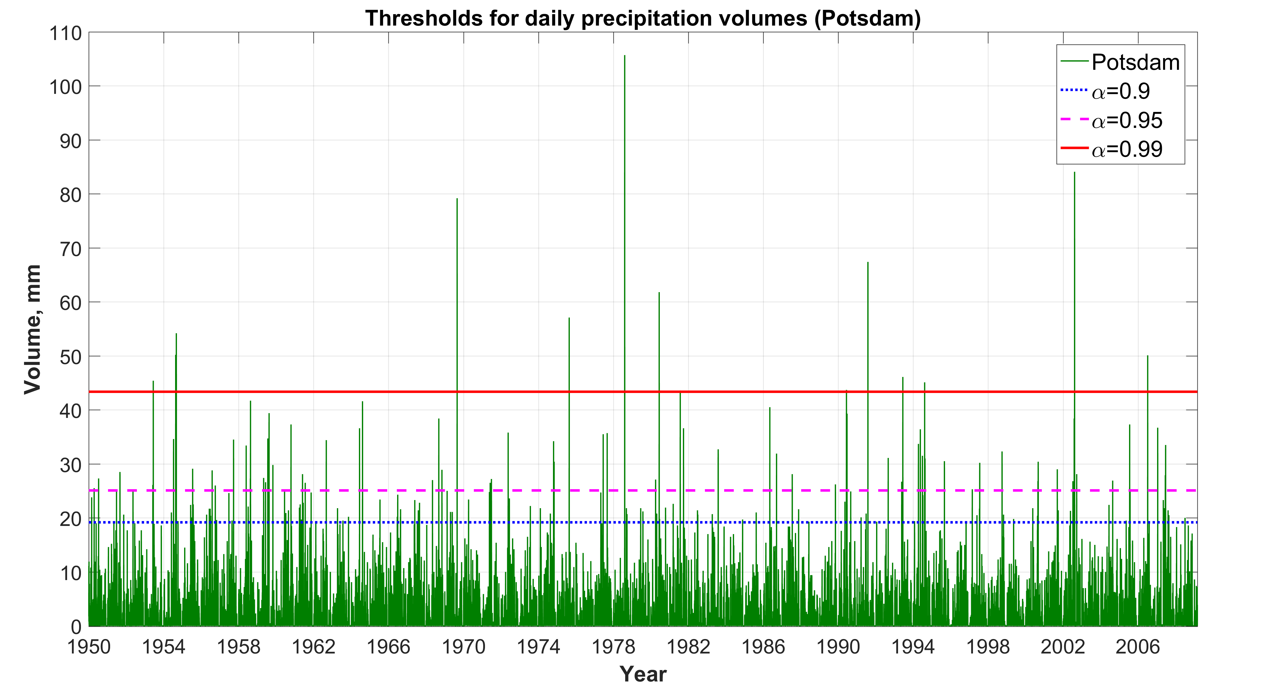
a)

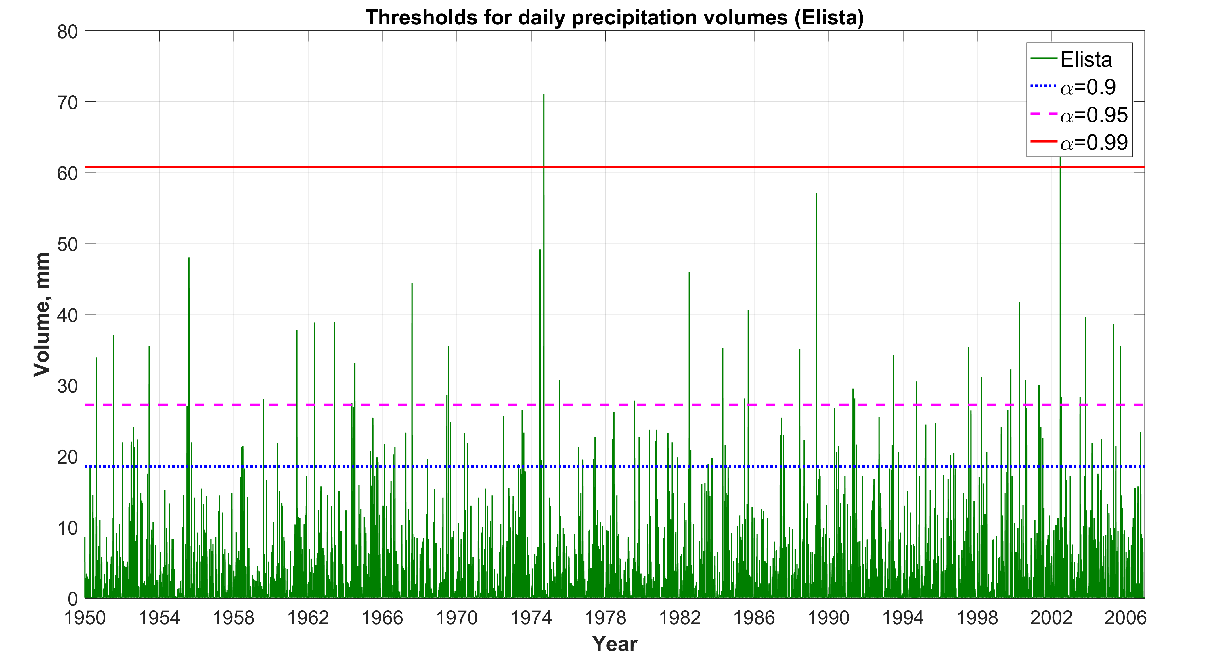
b)

Figure 1: Testing maximum daily precipitation within a wet period for abnormal heaviness: a) Potsdam; b) Elista, all data.

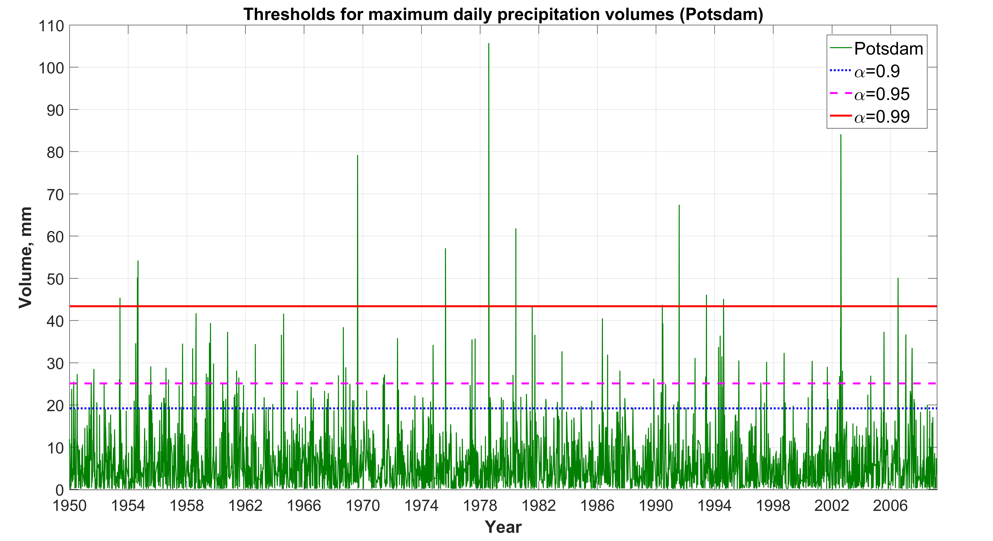
a)

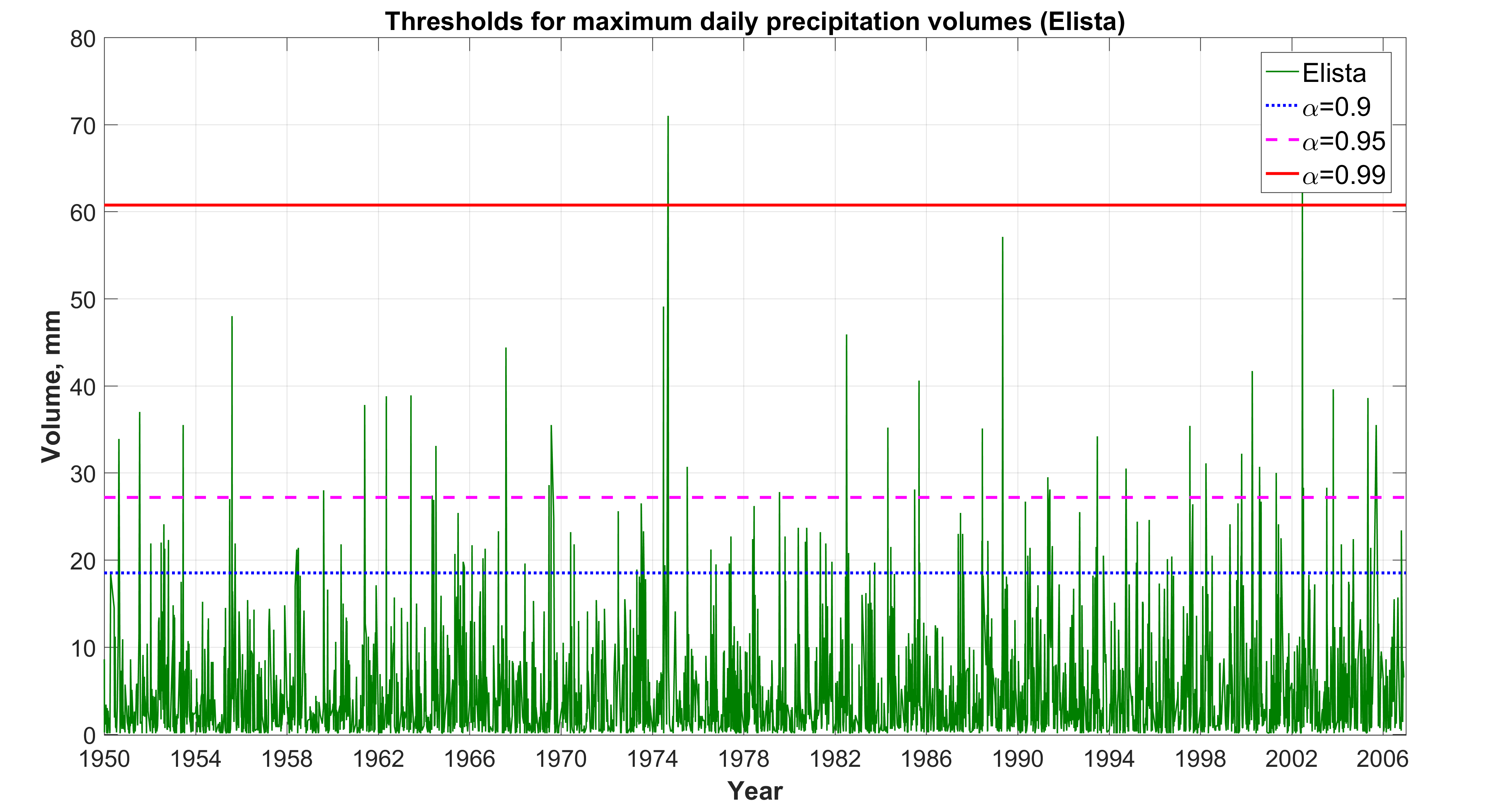
b)

Figure 2: Testing maximum daily precipitation within a wet period for abnormal heaviness: a) Potsdam; b) Elista, data containing only maximum daily precipitation for every wet period.

Fig. 1 contains all data. For the sake of vividness, on Fig. 2 only one, maximum, daily precipitation is exposed for each wet period. From Fig. 2 it is seen that during $58$ years (from $1950$ to $2007$) in Potsdam there were $13$ wet periods containing anomalously heavy maximum daily precipitation volumes (at $99\%$ threshold) and $69$ wet periods containing anomalously heavy maximum daily precipitation volumes (at $95\%$ threshold). Other maxima were ‘regular’. During the same period in Elista there were only $2$ wet periods containing anomalously heavy maximum daily precipitation volumes (at $99\%$ threshold) and $4$0 wet periods containing anomalously heavy maximum daily precipitation volumes (at $95\%$ threshold). Other maxima were ‘regular’. The proportion of abnormal maxima exceeding $99\%$ and $95\%$ thresholds in Potsdam is quite adequate (the latter is approximately five times greater than the former) whereas in Elista this proportion is noticeably different. Perhaps, this can be explained by the fact that, for Elista, heavy rains are rare events.

3 The tests for a total precipitation volume to be anomalously extremal based on the homogeneity test of a sample from the gamma distribution

3.1 The tests based on the beta and Snedecor–Fisher distributions

Here we will propose some algorithms of testing the hypotheses that a total precipitation volume during a wet period is anomalously extremal within a certain time horizon. Moreover, our approach makes it possible to consider relatively anomalously extremal volumes and absolutely anomalously extremal volumes for a given time horizon.

Let $m\in\mathbb{N}$ and $G^{(1)}_{r,\mu},G^{(2)}_{r,\mu},\ldots,G^{(m)}_{r,\mu}$ – be independent r.v.’s having the same gamma distribution with shape parameter $r>0$ and scale parameter $\mu>0$. In [15] it was suggested to use the distribution of the ratio

$$R^{*}=\frac{G^{(1)}_{r,\mu}}{G^{(1)}_{r,\mu}+G^{(2)}_{r,\mu}+\ldots+G^{(m)}_{r,\mu}}\stackrel{{\scriptstyle d}}{{=}}\frac{G^{(1)}_{r,1}}{G^{(1)}_{r,1}+G^{(2)}_{r,1}+\ldots+G^{(m)}_{r,1}}$$

as a heuristic model of the distribution of the extremely large precipitation volume based on the assumption that fluctuations of daily precipitation follow the gamma distribution. The gamma model for the distribution of daily precipitation volume is less adequate than the Pareto one [4]. Here we will modify the technique proposed in [15] and make it more adequate and justified.

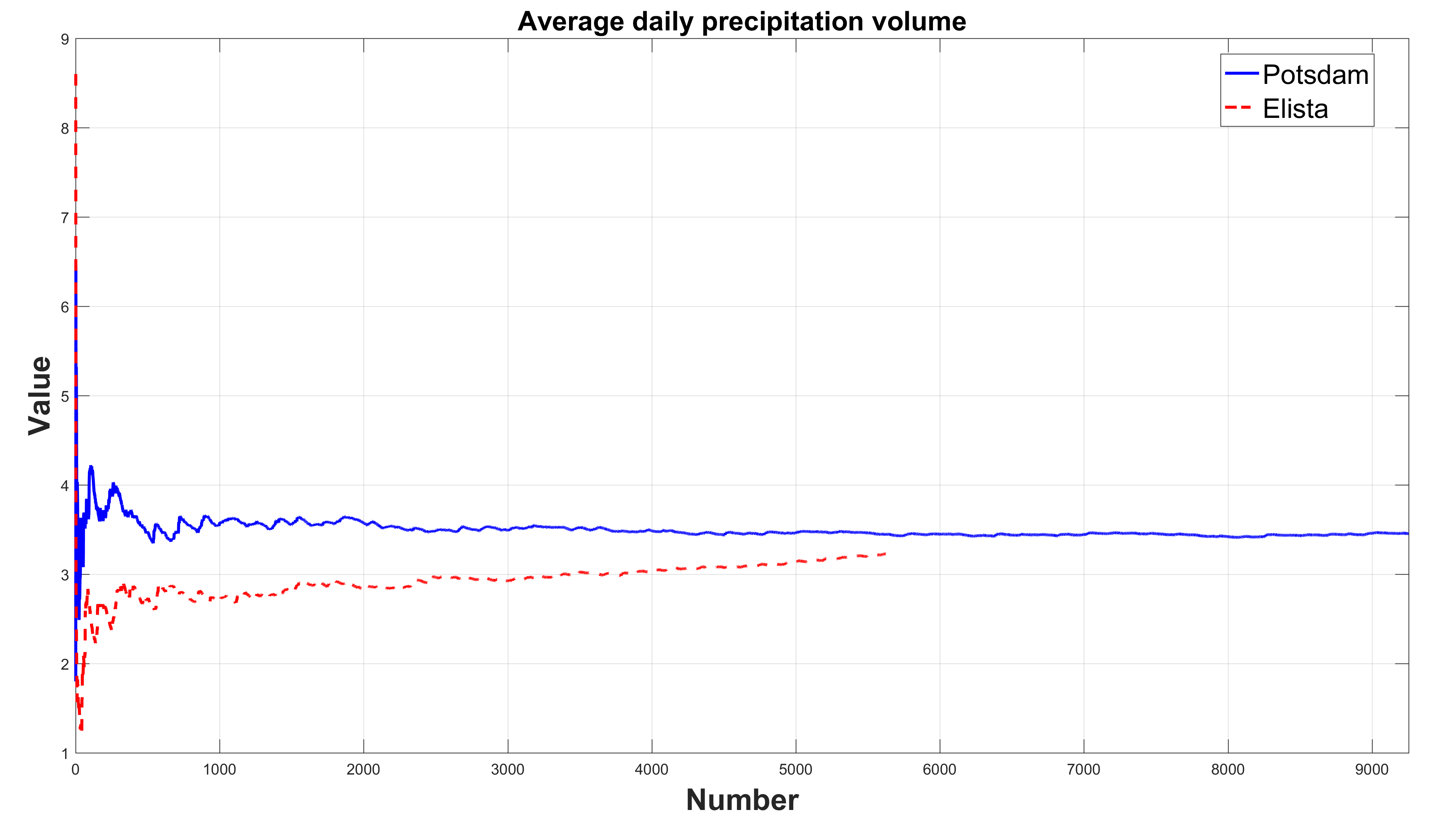
Figure 3: Stabilization of the cumulative averages of daily precipitation volumes as $n$ grows in Potsdam (continuous line) and Elista (dash line).

Let $X_{1},X_{2},\ldots$ be daily precipitation volumes on wet days. For $k\in\mathbb{N}$ denote $S_{k}=X_{1}+\ldots+X_{k}$. The statistical analysis of the observed data shows that the average daily precipitation volume on wet days is finite:

$$\frac{1}{n}\sum\limits_{j=1}^{n}X_{j}\Longrightarrow a\in(0,\infty).$$ (10)

Here the symbol $\Longrightarrow$ denotes the convergence in distribution.

Fig. 3 illustrates the stabilization of the cumulative averages of daily precipitation volumes as $n$ grows in Potsdam (continuous line) and Elista (dash line), and thus, the practical validity of assumption (10). It should be emphasized that in (10) we do not assume that $X_{1},X_{2},\ldots$ are independent.

Let $r>0$, $\mu>0$, $q\in(0,1)$, $n\in\mathbb{N}$. Let the r.v. $N_{r,p_{n}}$ have the negative binomial distribution with parameters $r$ and $p_{n}=\min\{q,\mu/n\}$. Using the properties of characteristic functions it is easy to make sure that

$$n^{-1}N_{r,p_{n}}\Longrightarrow G_{r,\mu}\stackrel{{\scriptstyle d}}{{=}}{\textstyle\frac{1}{\mu}}G_{r,1}$$ (11)

as $n\to\infty$. From (11) and From (11) and the transfer theorem for random sequences with independent random indices (see [7, 8]) we obtain the following analog of the law of large numbers for negative binomial random sums which can be actually regarded as a generalization of the Rényi theorem concerning the rarefaction of renewal processes.

Theorem 1

Assume that the daily precipitation volumes on wet days $X_{1},X_{2},...$ satisfy condition (10). Let the numbers $r>0$, $q\in(0,1)$ and $\mu>0$ be arbitrary. For each $n\in\mathbb{N}$, let the r.v. $N_{r,p_{n}}$ have the negative binomial distribution with parameters $r$ and $p_{n}=\min\{q,\mu/n\}$. Assume that the r.v.’s $N_{r,p_{n}}$ are independent of the sequence $X_{1},X_{2},...$ Then

$$n^{-1}S_{N_{r,p_{n}}}\Longrightarrow aG_{r,\mu}\stackrel{{\scriptstyle d}}{{=}}{\textstyle\frac{a}{\mu}}G_{r,1}$$

as $n\to\infty$.

Therefore, with the account of the excellent fit of the negative binomial model for the duration of a wet period [4], with rather small $p_{n}$, the gamma distribution can be regarded as an adequate and theoretically well-based model for the total precipitation volume during a (long enough) wet period. This theoretical conclusion based on the negative binomial model for the distribution of duration of a wet period is vividly illustrated by the empirical data as shown on Fig. 4 where the histograms of total precipitation volumes in Potsdam and Elista and the fitted gamma distributions are shown. For comparison, the densities of the best generalized Pareto distributions are also presented. It can be seen that even the best fitted Pareto distributions demonstrate worse fit than the gamma distribution.

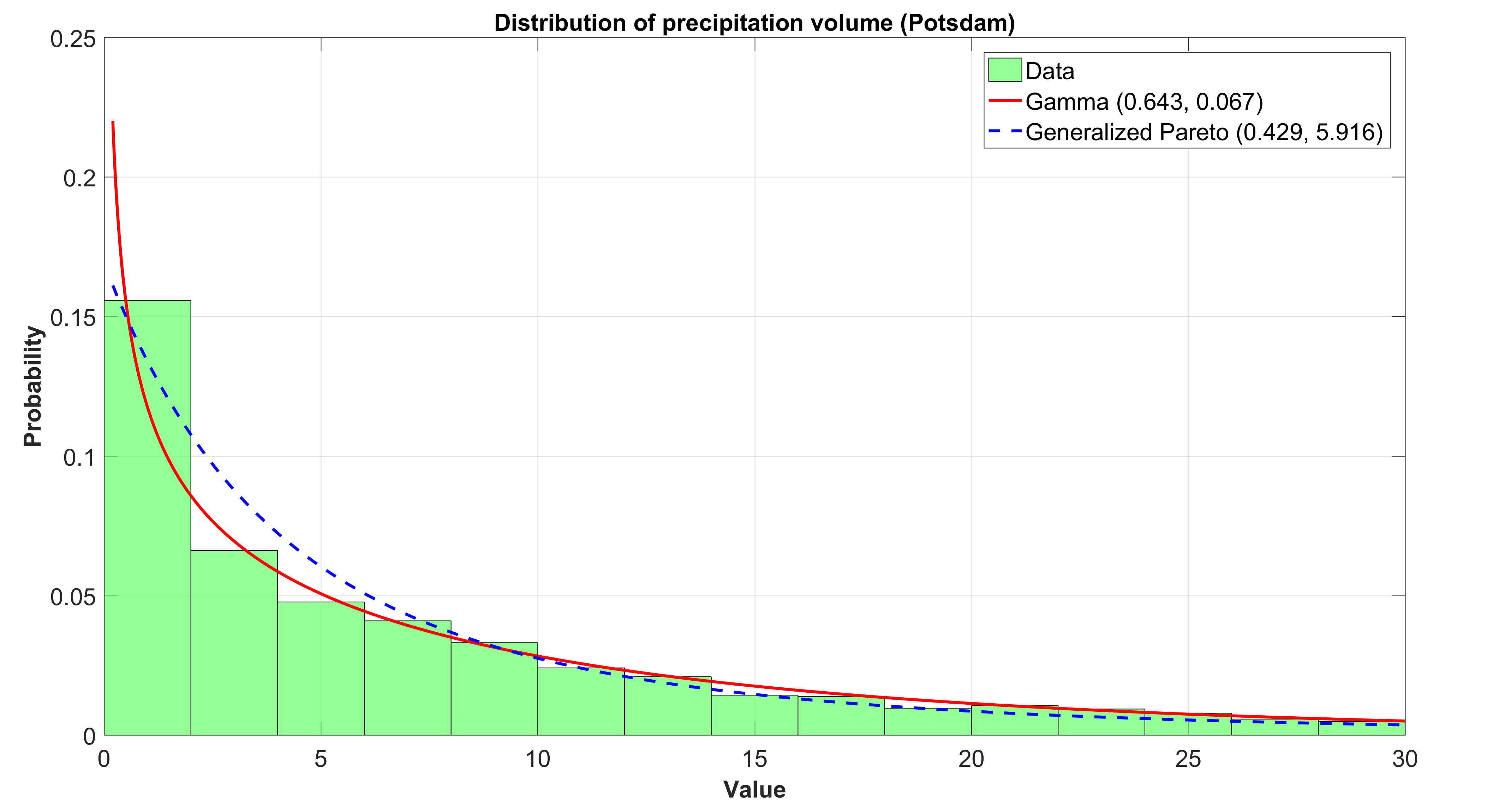
a)

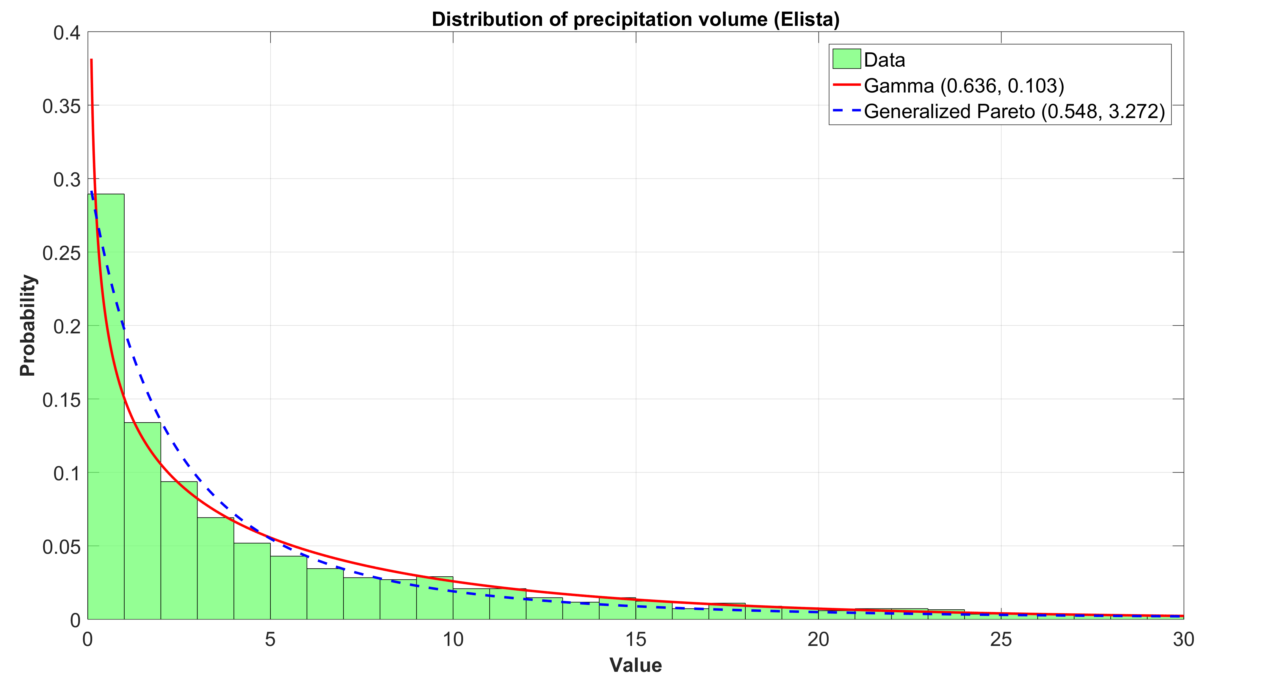
b)

Figure 4: The histograms of total precipitation volumes in Potsdam (a) and Elista (b) and the fitted gamma and generalized Pareto distributions.

Let $m\in\mathbb{N}$ and $G^{(1)}_{r,\mu},G^{(2)}_{r,\mu},\ldots,G^{(m)}_{r,\mu}$ be independent r.v.’s having the same gamma distribution with parameters $r>0$ and $\mu>0$. Consider the relative contribution of the r.v. $G^{(1)}_{r,\mu}$ to the sum $G^{(1)}_{r,\mu}+G^{(2)}_{r,\mu}+\ldots+G^{(m)}_{r,\mu}$:

$$R=\frac{G^{(1)}_{r,\mu}}{G^{(1)}_{r,\mu}+G^{(2)}_{r,\mu}+\ldots+G^{(m)}_{r,\mu}}\stackrel{{\scriptstyle d}}{{=}}\frac{G^{(1)}_{r,1}}{G^{(1)}_{r,1}+G^{(2)}_{r,1}+\ldots+G^{(m)}_{r,1}}\stackrel{{\scriptstyle d}}{{=}}$$

$$\stackrel{{\scriptstyle d}}{{=}}\bigg{(}1+\frac{1}{G^{(1)}_{r,1}}(G^{(2)}_{r,1}+\ldots+G^{(m)}_{r,1})\bigg{)}^{-1}\stackrel{{\scriptstyle d}}{{=}}\bigg{(}1+\frac{G_{(m-1)r,1}}{G_{r,1}}\bigg{)}^{-1},$$ (12)

where the gamma-distributed r.v.’s on the right hand side are independent. So, the r.v. $R$ characterizes the relative precipitation volume for one (long enough) wet period with respect to the total precipitation volume registered for $m$ wet periods.

The distribution of the r.v. $R$ is completely determined by the distribution of the ratio of two independent gamma-distributed r.v.’s. To find the latter, denote $k=(m-1)r$ and obtain

$$\frac{G_{k,1}}{G_{r,1}}=\frac{k}{r}\cdot\bigg{(}\frac{r}{k}\cdot\frac{G_{k,1}}{G_{r,1}}\bigg{)}\stackrel{{\scriptstyle d}}{{=}}\frac{k}{r}\cdot Q_{k,r},$$

where $Q_{k,r}$ is the r.v. having the Snedecor–Fisher distribution determined for $k>0$, $r>0$ by the Lebesgue density

$$f_{k,r}(x)=\frac{\Gamma(k+r)}{\Gamma(k)\Gamma(r)}\Big{(}\frac{k}{r}\Big{)}^{k}\frac{x^{k-1}}{(1+\frac{k}{r}x)^{k+r}},\ \ \ x\geqslant 0,$$ (13)

(as is known, $Q_{k,r}\stackrel{{\scriptstyle d}}{{=}}rG_{k,\,1}(kG_{r,\,1})^{-1}$, where the r.v.’s $G_{k,\,1}$ and $G_{r,\,1}$ are independent (see, e. g., [5], p. 32)). It should be noted that the particular value of the scale parameter is insignificant. For convenience, it is assumed equal to one.

So, $R\stackrel{{\scriptstyle d}}{{=}}\big{(}1+\frac{k}{r}Q_{k,r}\big{)}^{-1}$, and, as is easily made sure by standard calculation using (13), the distribution of the r.v. $R$ is determined by the density

$$p(x;k,r)=\frac{\Gamma(k+r)}{\Gamma(r)\Gamma(k)}(1-x)^{k-1}x^{r-1},\ \ \ \ 0\leqslant x\leqslant 1,$$

that is, it is the beta distribution with parameters $k=(m-1)r$ and $r$.

Then the test for the homogeneity of an independent sample of size $m$ consisting of the gamma-distributed observations of total precipitation volumes during $m$ wet periods with known $\gamma$ based on the r.v. $R$ looks as follows. Let $V_{1},\ldots,V_{m}$ be the total precipitation volumes during $m$ wet periods and, moreover, $V_{1}\geqslant V_{j}$ for all $j\geqslant 2$. Calculate the quantity

$$SR=\frac{V_{1}}{V_{1}+\ldots+V_{m}}$$

($SR$ means ‘‘$S$ample $R$’’). From what was said above it follows that under the hypothesis $H_{0}$: ‘‘the precipitation volume $V_{1}$ under consideration is not anomalously large’’ the r.v. $SR$ has the beta distribution with parameters $k=(m-1)r$ and $r$. Let $\varepsilon\in(0,1)$ be a small number, $\beta_{k,r}(1-\varepsilon)$ be the $(1-\varepsilon)$-quantile of the beta distribution with parameters $k=(m-1)r$ and $r$. If $SR>\beta_{k,r}(1-\varepsilon)$, then the hypothesis $H_{0}$ must be rejected, that is, the volume $V_{1}$ of precipitation during one wet period must be regarded as anomalously large. Moreover, the probability of erroneous rejection of $H_{0}$ is equal to $\varepsilon$.

Instead of $R$ (12), the quantity

$$R_{0}=\frac{(m-1)G^{(1)}_{r,\mu}}{G^{(2)}_{r,\mu}+\ldots+G^{(m)}_{r,\mu}}\stackrel{{\scriptstyle d}}{{=}}\frac{k}{r}\frac{G_{r,\mu}}{G_{k,\mu}}\stackrel{{\scriptstyle d}}{{=}}\frac{k}{r}\frac{G_{r,1}}{G_{k,1}}\stackrel{{\scriptstyle d}}{{=}}Q_{r,k}$$

can be considered. Then, as is easily seen, the r.v.’s $R$ and $R_{0}$ are related by the one-to-one correspondence

$$R=\frac{R_{0}}{m-1+R_{0}}\ \ \text{\rm or}\ \ R_{0}=\frac{(m-1)R}{1-R},$$

so that the homogeneity test for a sample from the gamma distribution equivalent to the one described above and, correspondingly, the test for a precipitation volume during a wet period to be anomalously large, can be based on the r.v. $R_{0}$ which has the Snedecor–Fisher distribution with parameters $r$ and $k=(m-1)r$.

Namely, again let $V_{1},\ldots,V_{m}$ be the total precipitation volumes during $m$ wet periods and, moreover, $V_{1}\geqslant V_{j}$ for all $j\geqslant 2$. Calculate the quantity

$$SR_{0}=\frac{(m-1)V_{1}}{V_{2}+\ldots+V_{m}}$$

($SR_{0}$ means ‘‘$S$ample $R_{0}$’’). From what was said above it follows that under the hypothesis $H_{0}$: ‘‘the precipitation volume $V_{1}$ under consideration is not anomalously large’’ the r.v. $SR$ has the Snedecor–Fisher distribution with parameters $r$ и $k=(m-1)r$. Let $\varepsilon\in(0,1)$ be a small number, $q_{r,k}(1-\varepsilon)$ be the $(1-\varepsilon)$-quantile of the Snedecor–Fisher distribution with parameters $r$ и $k=(m-1)r$. If $SR_{0}>q_{r,k}(1-\varepsilon)$, then the hypothesis $H_{0}$ must be rejected, that is, the volume $V_{1}$ of precipitation during one wet period must be regarded as anomalously large. Moreover, the probability of erroneous rejection of $H_{0}$ is equal to $\varepsilon$.

Let $l$ be a natural number, $1\leqslant l<m$. It is worth noting that, unlike the test based on the statistic $R$, the test based on $R_{0}$ can be modified for testing the hypothesis $H_{0}^{\prime}$: ‘‘the precipitation volumes $V_{i_{1}},V_{i_{2}},\ldots,V_{i_{l}}$ do not make an anomalously large cumulative contribution to the total precipitation volume $V_{1}+\ldots+V_{m}$’’. For this purpose denote

$$T_{l}=V_{i_{1}}+V_{i_{2}}+\ldots+V_{i_{l}},\ \ \ \ T=V_{1}+V_{2}+\ldots+V_{m}$$

and consider the quantity

$$SR_{0}^{\prime}=\frac{(m-l)T_{l}}{l(T-T_{l})}.$$

In the same way as it was done above, it is easy to make sure that

$$SR_{0}^{\prime}\stackrel{{\scriptstyle d}}{{=}}\frac{(m-l)G_{lr,l}}{lG_{(m-l)r,1}}\stackrel{{\scriptstyle d}}{{=}}Q_{lr,(m-l)r}.$$

Let $\varepsilon\in(0,1)$ be a small number, $q_{lr,(m-1)r}(1-\varepsilon)$ be the $(1-\varepsilon)$-quantile of the Snedecor–Fisher distribution with parameters $lr$ и $k=(m-l)r$. If $SR_{0}^{\prime}>q_{lr,(m-l)r}(1-\varepsilon)$, then the hypothesis $H_{0}^{\prime}$ must be rejected, that is, the cumulative contribution of the precipitation volumes $V_{i_{1}},V_{i_{2}},\ldots,V_{i_{l}}$ into the total precipitation volume $V_{1}+\ldots+V_{m}$ must be regarded as anomalously large. Moreover, the probability of erroneous rejection of $H_{0}^{\prime}$ is equal to $\varepsilon$.

The examples of application of the test for a total precipitation volume within a wet period to be anomalously large will be discussed in Section 3.3.

3.2 Determination of abnormalities types based on the results of the statistical analysis

In this section we present the results of the application of the test $SR_{0}$ to the analysis of the time series of daily precipitation observed in Potsdam and Elista from $1950$ to $2009$.

First of all it should be emphasized that the parameter $m$ of the Snedecor–Fisher distribution of the test statistic $SR_{0}$ is tightly connected with the time horizon, the abnormality of precipitation within which is studied. Indeed, the average duration of a wet/dry period (or, which is the same, the average distance between the first days of successive wet periods) in Potsdam turns out to be $5.804\approx 6$ days. So, one observation of a total precipitation during a wet period, on the average, corresponds to approximately 6 days. This means, that, for example, the value $m=5$ corresponds to approximately one month on the time axis, the value $m=15$ corresponds to approximately 3 months (a season), the value $m=60$ corresponds to approximately one year.

Second, it is important that the test for a total precipitation volume during one wet period to be anomalously large can be applied to the observed time series in a moving mode. For this purpose a window (a set of successive observations) should be determined. The number of observations in this set, say, $m$, is called the window width. The observations within a window constitute the sample to be analyzed. After the test has been performed for a given position of the window, the window moves rightward by one observation so that the leftmost observation at the previous position of the window is excluded from the sample and the observation next to the rightmost observation is added to the sample. The test is performed once more and so on. It is clear that each fixed observation falls in exactly $m$ successive windows (from $m$th to $N-m+1$, where $N$ denotes the number of wet periods). Two cases are possible: (i) the fixed observation is recognized as anomalously large within each of $m$ windows containing this observation and (ii) the fixed observation is recognized as anomalously large within at least one of $m$ windows containing this observation. In the case (i) the observation will be called absolutely anomalously large with respect to a given time horizon (approximately equal to $m\cdot 5.804\approx 6m$ days). In the case (ii) the observation will be called relatively anomalously large with respect to a given time horizon. Of course, these definitions admit intermediate cases where the observation is recognized as anomalously large for $q\cdot m$ windows with $q\in[\frac{1}{m},1]$.

3.3 The examples of statistical analysis of total precipitation volumes

The results of the application of the test for a total precipitation volume during one wet period to be anomalously large based on $SR_{0}$ in the moving mode are shown on Figs. 5–7 (Potsdam) and 8–10 (Elista) for different time horizons ($30$, $90$ and $360$ days). The notation $Extr_{int}$ corresponds to the intermediate extremes (the fixed observation is recognized as anomalously large within at least $\lceil m/2\rceil$ windows containing this observation, here the symbol $\lceil\cdot\rceil$ denotes the next larger integer).

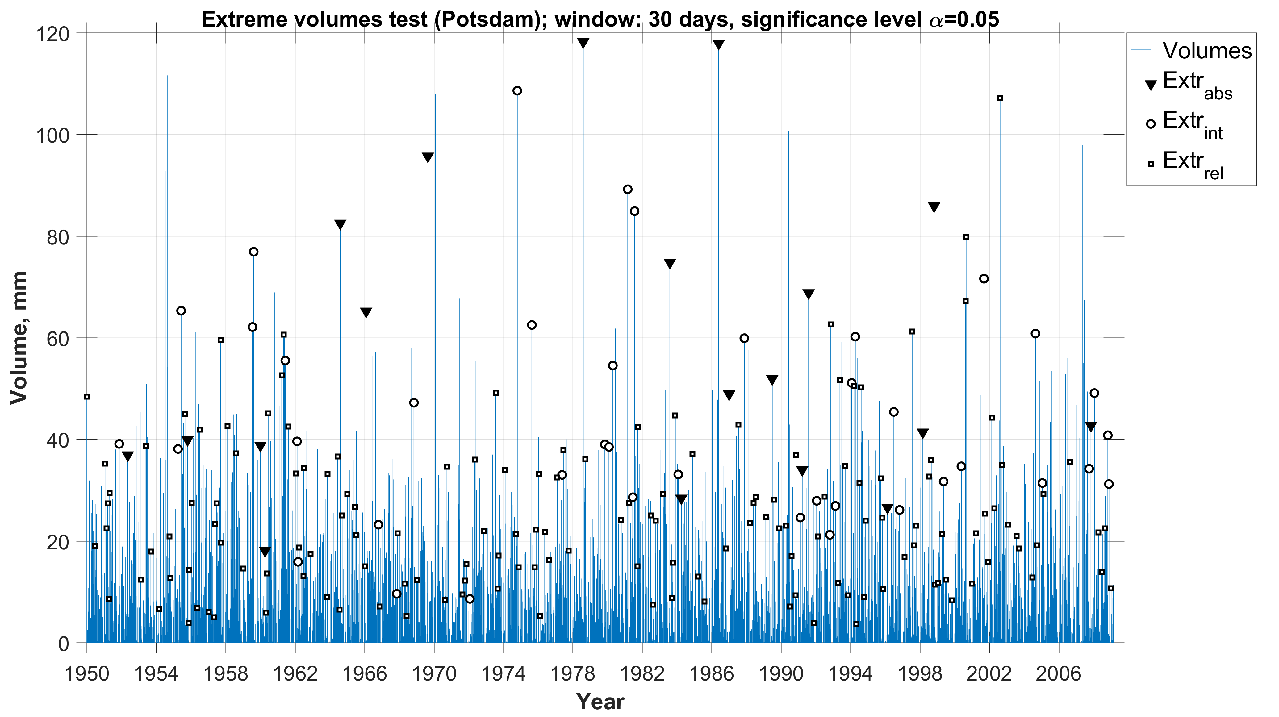
a)

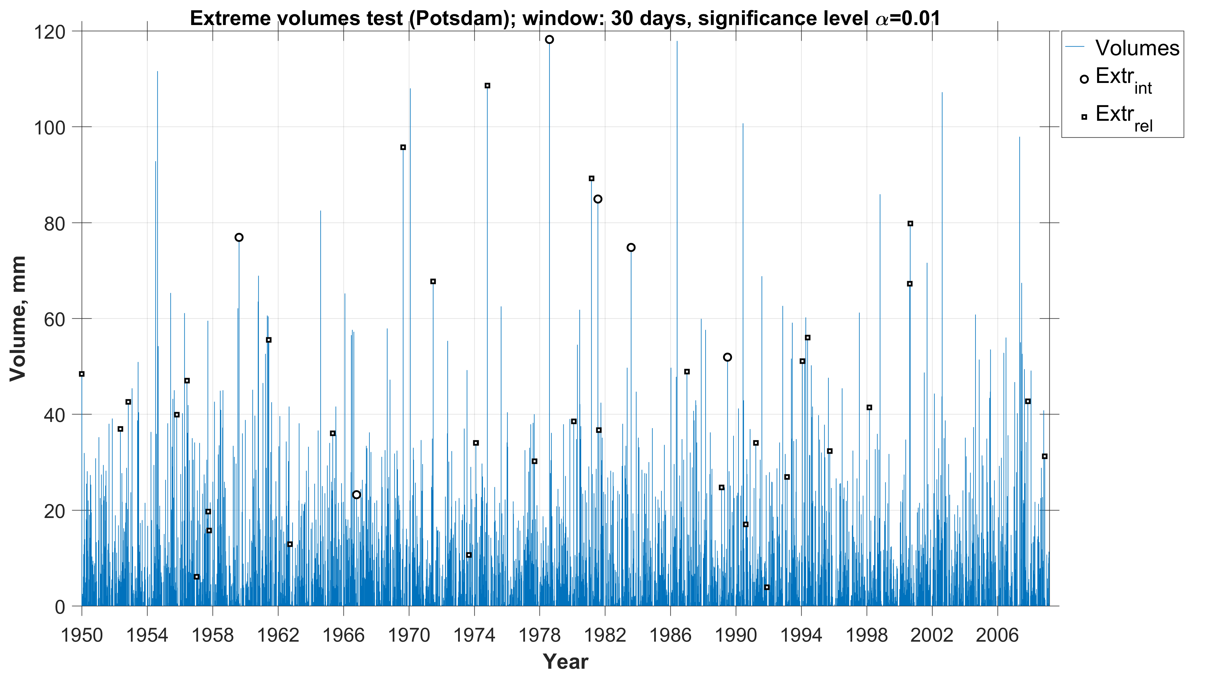
b)

Figure 5: Absolutely (triangles), relatively (squares) and intermediate (circles) abnormal precipitation volumes, Potsdam, time horizon = 30 days, significance levels $\alpha=0.05$ (a) and $\alpha=0.01$ (b).

It is seen that at relatively small time horizons the test yields non-trivial and unobvious conclusions. However, as the time horizon increases, the results of the test become more expected. At small time horizons there are some big precipitation volumes that are not recognized as abnormal. At large time horizons there are almost no ‘regular’ big precipitation volumes at significance level $\alpha=0.05$ whereas at the smaller significance level $\alpha=0.01$ there are some ‘regular’ big precipitation volumes which are thus not recognized as abnormal.

a)

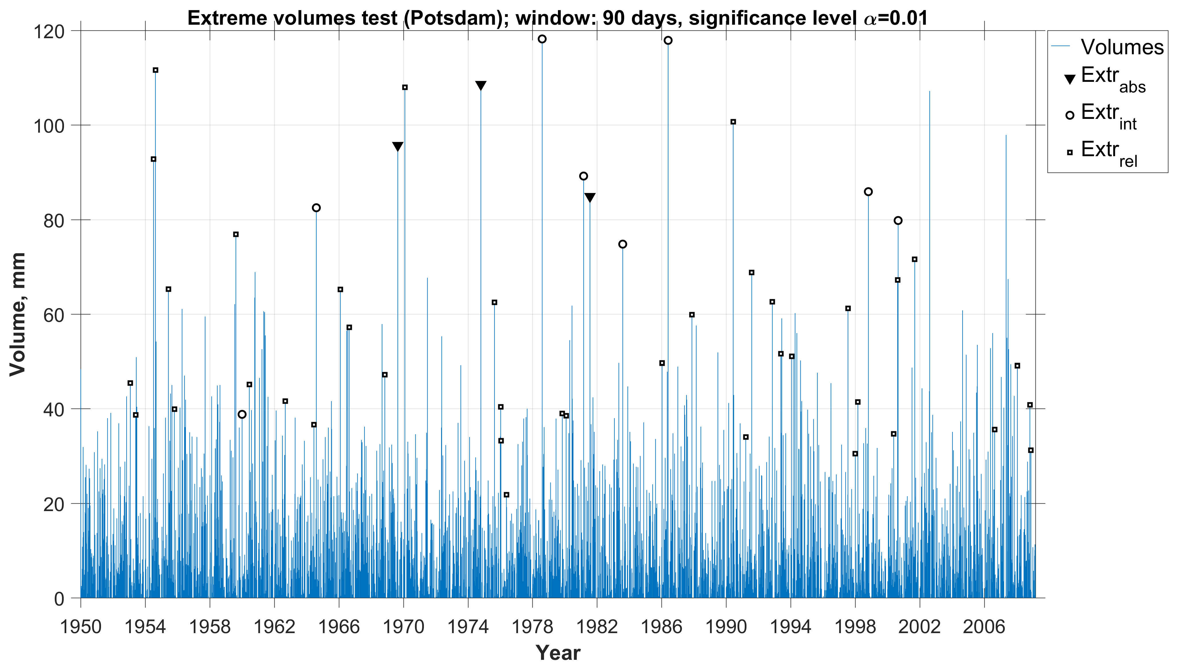
b)

Figure 6: Absolutely (triangles), relatively (squares) and intermediate (circles) abnormal precipitation volumes, Potsdam, time horizon = 90 days, significance levels $\alpha=0.05$ (a) and $\alpha=0.01$ (b).

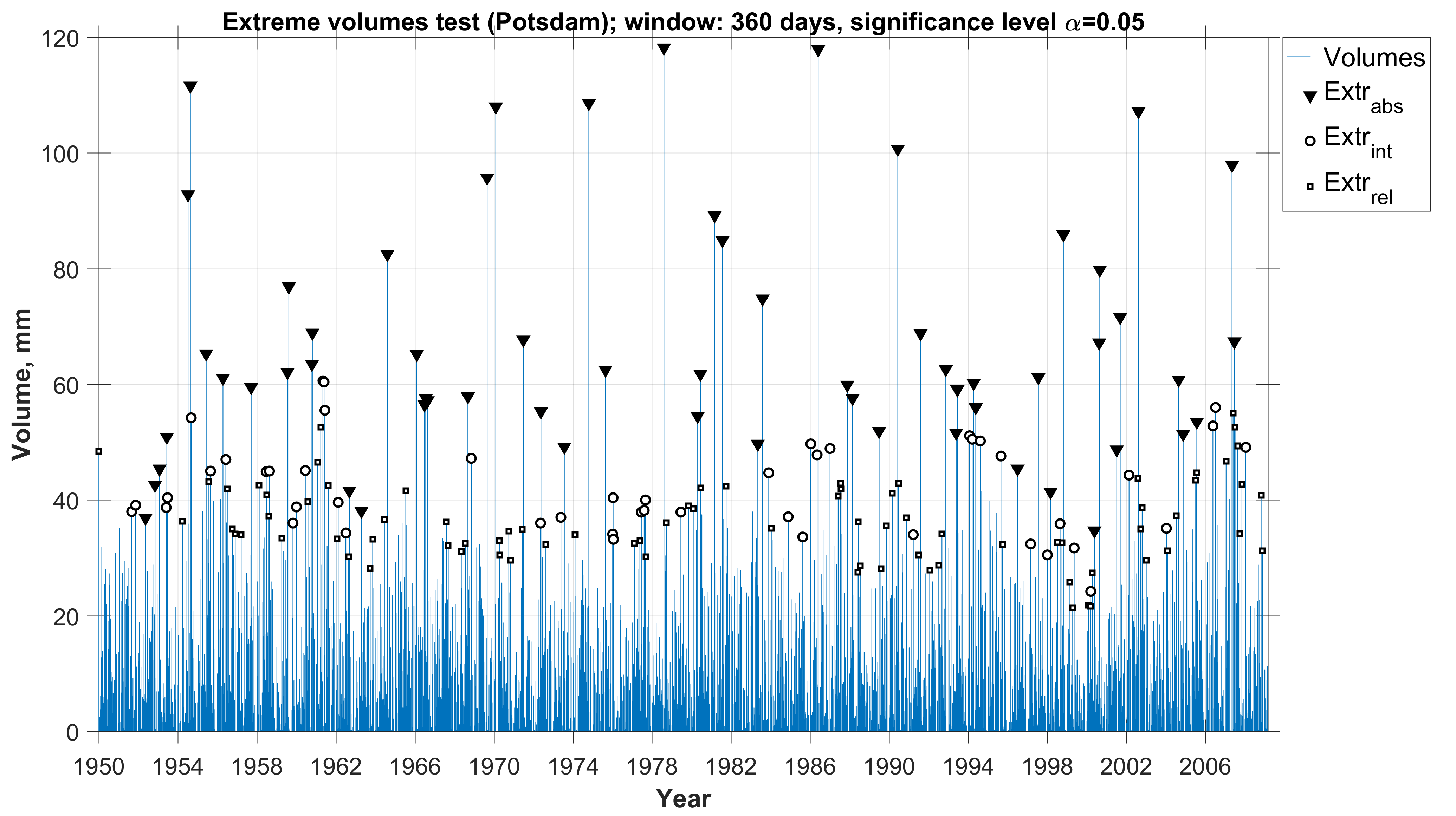
a)

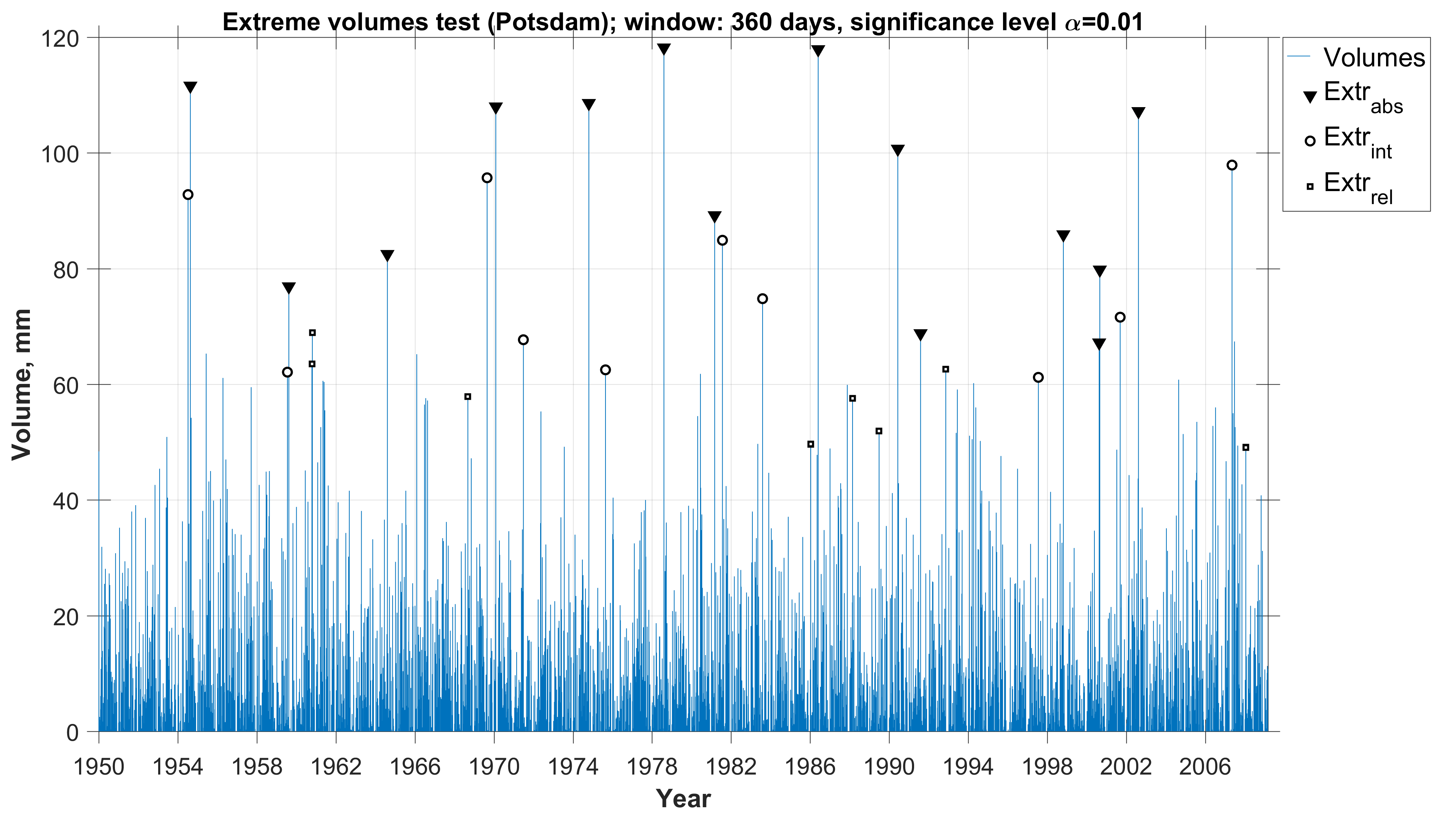
b)

Figure 7: Absolutely (triangles), relatively (squares) and intermediate (circles) abnormal precipitation volumes, Potsdam, time horizon = 360 days, significance levels $\alpha=0.05$ (a) and $\alpha=0.01$ (b).

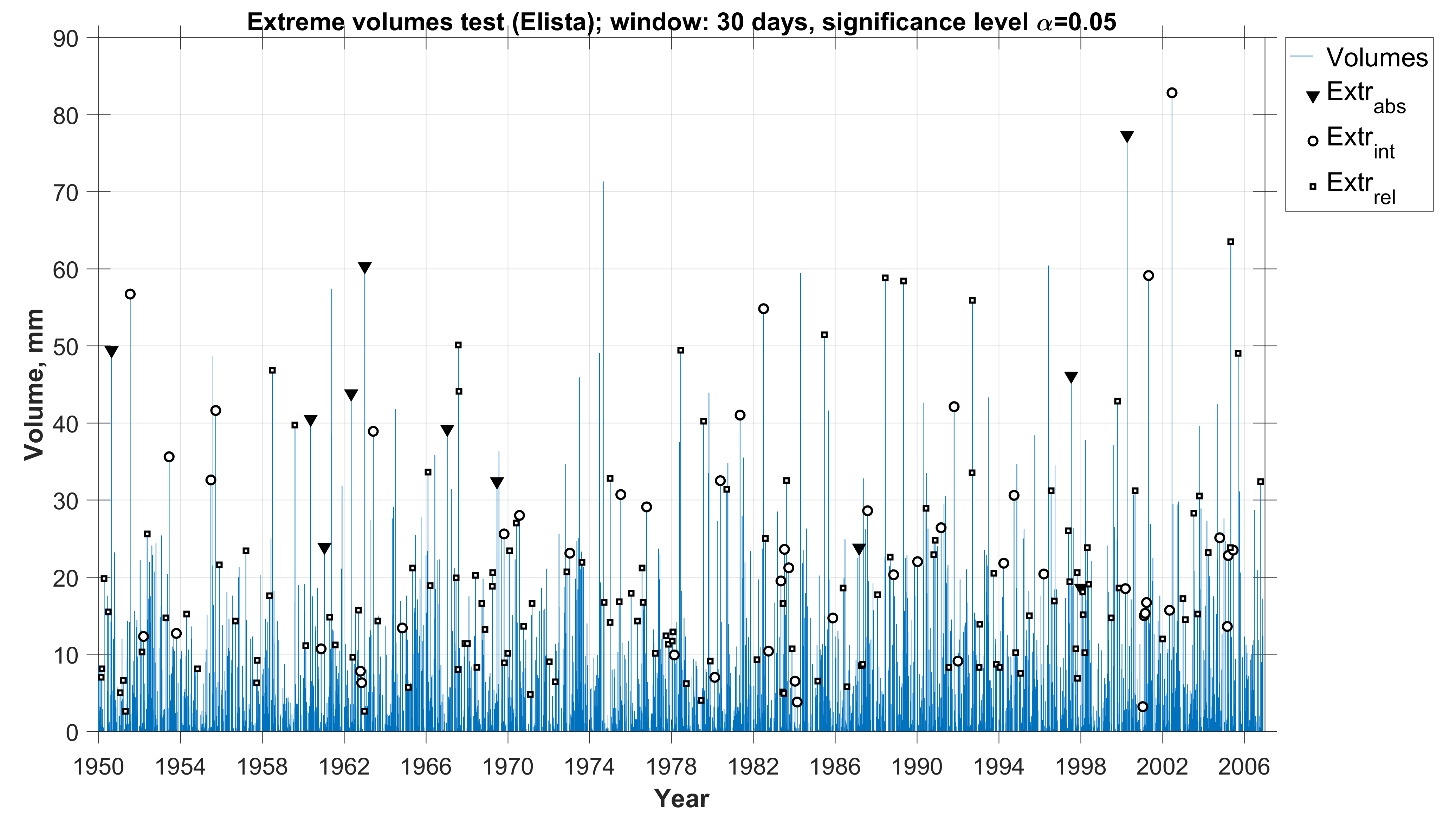
a)

b)

Figure 8: Absolutely (triangles), relatively (squares) and intermediate (circles) abnormal precipitation volumes, Elista, time horizon = 30 days, significance levels $\alpha=0.05$ (a) and $\alpha=0.01$ (b).

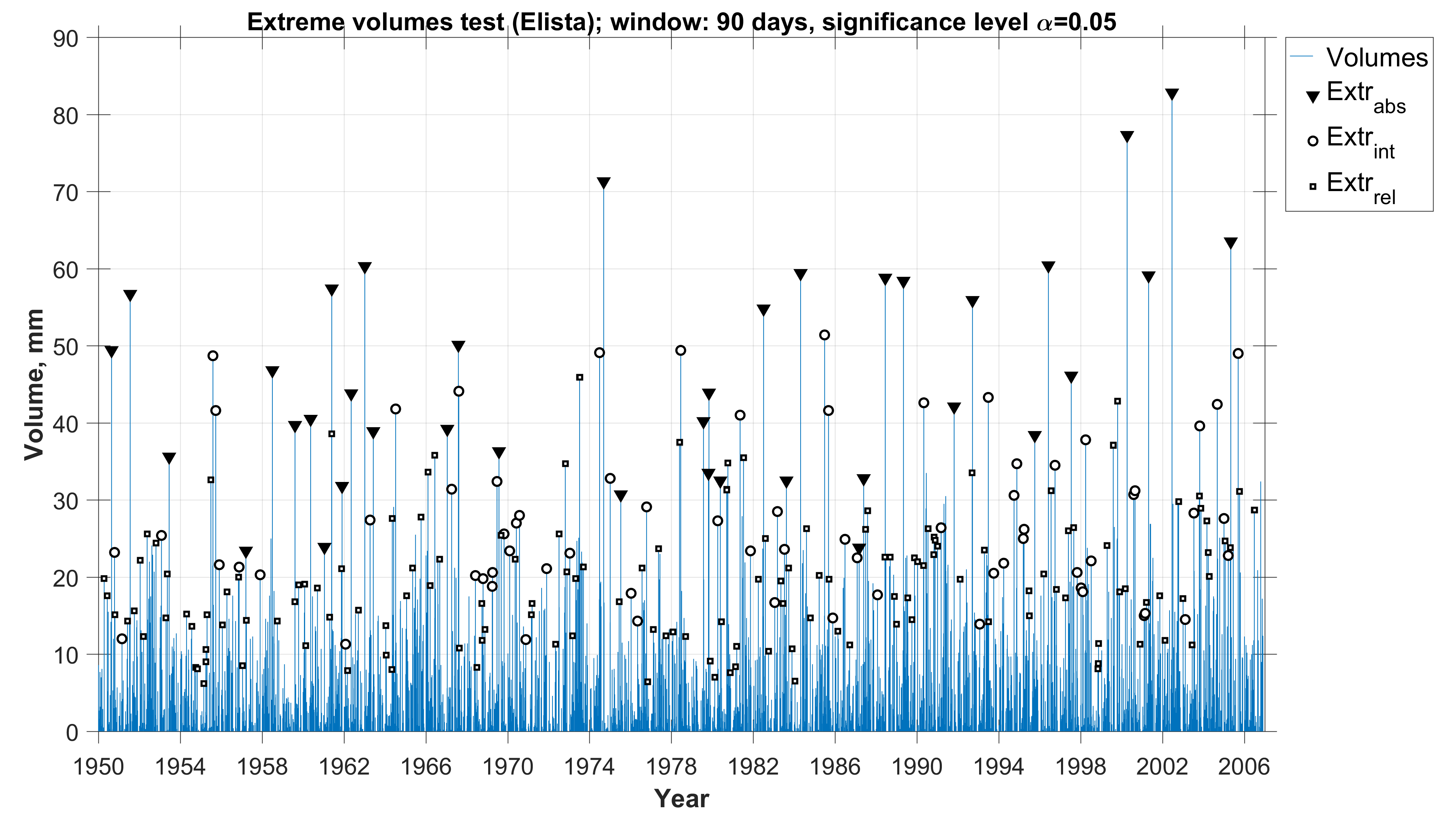
a)

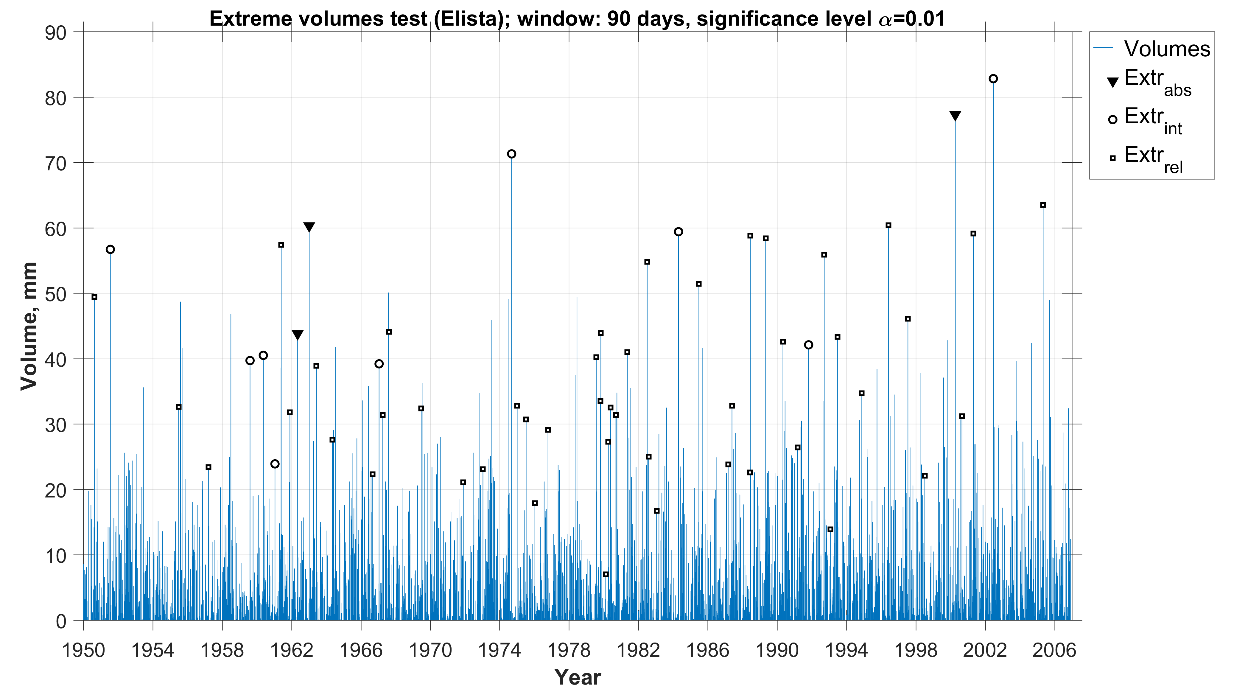
b)

Figure 9: Absolutely (triangles), relatively (squares) and intermediate (circles) abnormal precipitation volumes, Elista, time horizon = 90 days, significance levels $\alpha=0.05$ (a) and $\alpha=0.01$ (b).

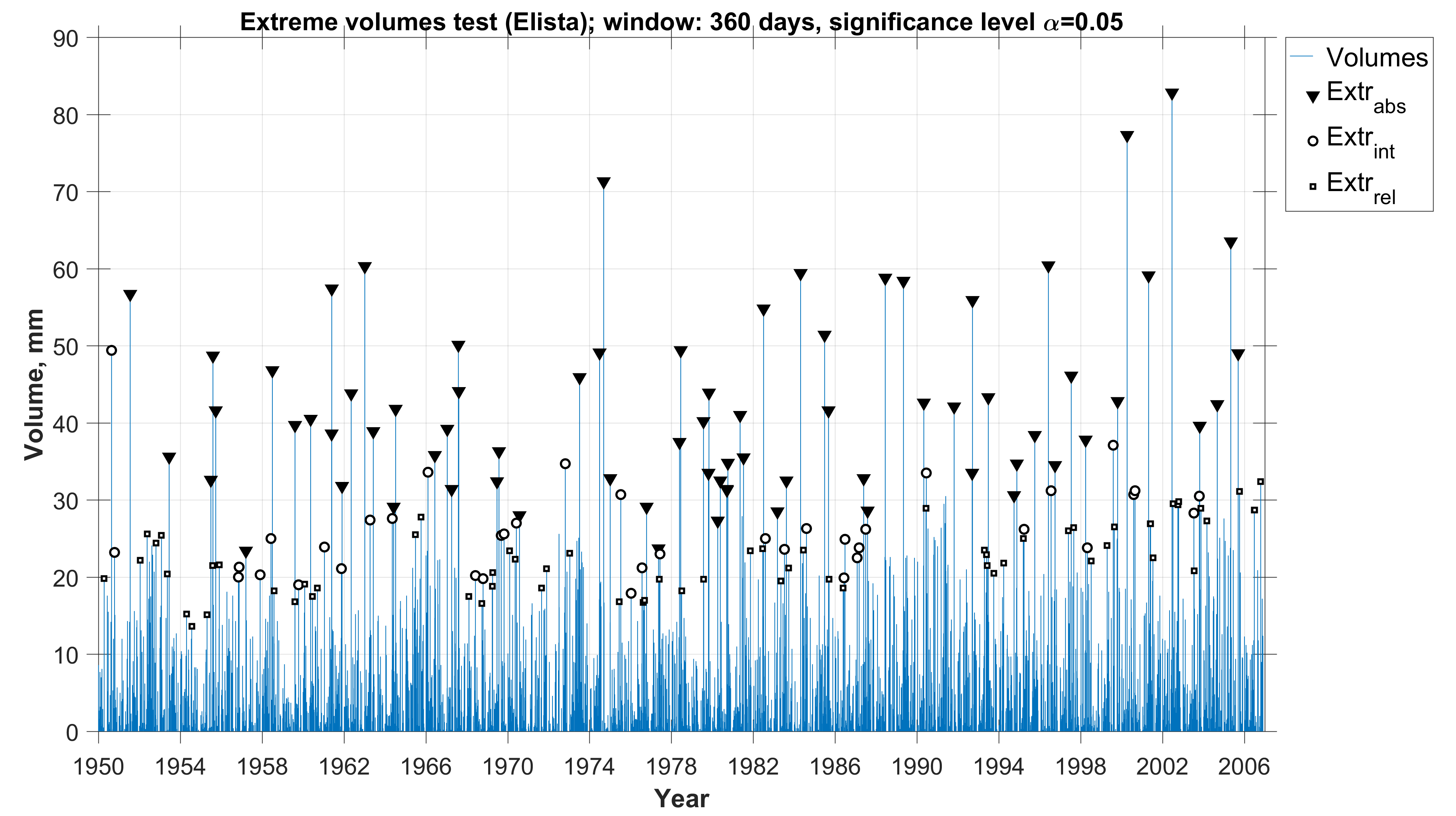
a)

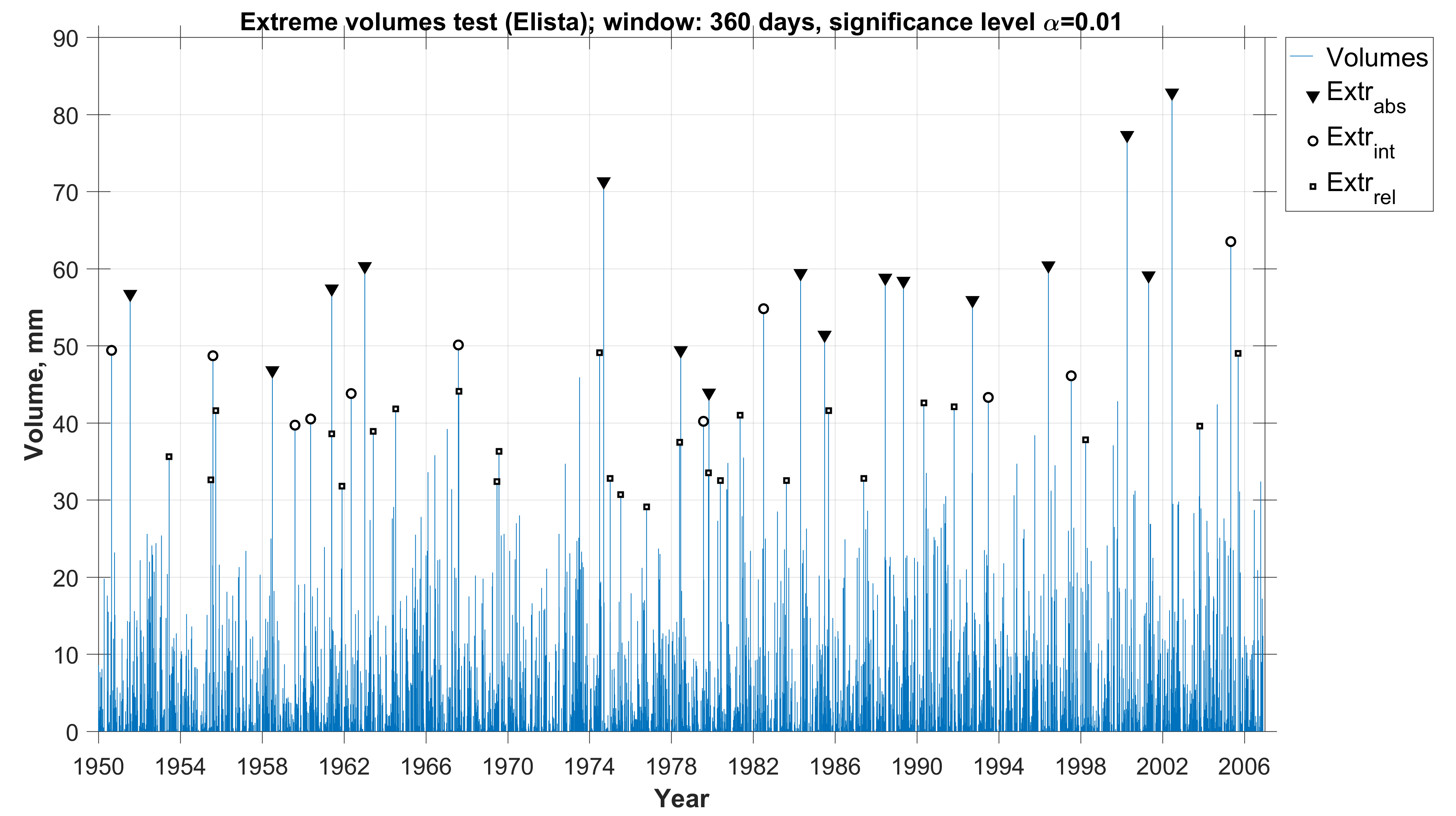
b)

Figure 10: Absolutely (triangles), relatively (squares) and intermediate (circles) abnormal precipitation volumes, Elista, time horizon = 360 days, significance levels $\alpha=0.05$ (a) and $\alpha=0.01$ (b).

4 Conclusions and discussion

This paper states that the negative binomial distribution may be fruitful for description of the really observed wet periods and can be applied to test of hypothesis that the specific precipitation volume considered over given wet period is anomalous. It is an important issue since now there is no single-valued criterion which precipitation volume is anomalous and which is not. Obviously that the same volume may be normal in one region where precipitations are quite frequent, for instance in tropical zone and absolutely anomalous in another one, for instance in desert. The proposed test considers the relative part of precipitation and is free from the aforementioned disadvantage. On the other hand, it gives the numerical method how to test this hypothesis that can be easily implemented. The considered scheme may be expanded for other geophysical variables such as wind speed, heat fluxes etc, both separately or jointly. This may be very important for global climate prediction models, for forecasting and evaluation of dangerous phenomena and processes.

- [1] P. Embrechts , K. Klüppelberg, T. Mikosch, Modeling Extremal Events, Springer, Berlin–New York, 1998.
- [2] A.K. Gorshenin, On some mathematical and programming methods for construction of structural models of information flows, Informatika i ee Primeneniya, 11 (1) (2017) 58–68.
- [3] A.K. Gorshenin, Pattern-based analysis of probabilistic and statistical characteristics of precipitations, Informatika i ee Primeneniya, 11 (4) (2017) 38–46.
- [4] A.K. Gorshenin, V.Yu. Korolev, Scale mixtures of Frechet distributions as asymptotic approximations of extreme precipitation, Journal of Mathematical Sciences, 234 (6) (2018) 886–903.
- [5] N.L. Johnson, S. Kotz, N. Balakrishnan, Continuous Univariate Distributions, Vol. 2 (2nd Edition), Wiley, New York, 1995.
- [6] J.F.C. Kingman, Poisson processes, Clarendon Press, Oxford, 1993.
- [7] V.Yu. Korolev, Convergence of random sequences with independent random indexes. I, Theory of Probability and its Applications, 39 (2) (1994) 313–333.
- [8] V.Yu. Korolev, Convergence of random sequences with independent random indexes. II // Theory of Probability and its Applications, 40 (4) (1995) 770–772.
- [9] V.Yu. Korolev, A.I. Zeifman, Convergence of statistics constructed from samples with random sizes to the Linnik and Mittag-Leffler distributions and their generalizations, Journal of Korean Statistical Society, 46 (2) (2017) 161–181.
- [10] V.Yu. Korolev, A.K. Gorshenin, S.K. Gulev, K.P. Belyaev, A.A. Grusho, Statistical Analysis of Precipitation Events, AIP Conference Proceedings, 1863 (2017) 090011.
- [11] V.Yu. Korolev, A.K. Gorshenin, The probability distribution of extreme precipitation’’, Doklady Earth Sciences, 477 (2) 1461–1466 (2017).
- [12] S. Kotz, I.V. Ostrovskii, A mixture representation of the Linnik distribution, Statistics and Probability Letters, 26 (1996) 61–64.
- [13] M. Lockhoff, O. Zolina, C. Simmer, J. Schulz, Evaluation of Satellite-Retrieved Extreme Precipitation over Europe using Gauge Observations, Journal of Climate, 27 (2) (2014) 607–623.
- [14] O. Zolina, C. Simmer, A. Kapala, S.K. Gulev, On the robustness of the estimates of centennial-scale variability in heavy precipitation from station data over Europe, Geophysical Research Letters, 32 (2005) L14707.
- [15] O. Zolina, C. Simmer, K. Belyaev, A. Kapala, S.K. Gulev, Improving estimates of heavy and extreme precipitation using daily records from European rain gauges, Journal of Applied Meteorology, 10 (2009) 701–716.
- [16] O. Zolina, C. Simmer, K. Belyaev, A. Kapala, S.K. Gulev, P. Koltermann, Changes in the duration of European wet and dry spells during the last 60 years, Journal of Climate, 26 (2013) 2022–2047.
- [17] O. Zolina, Multidecadal trends in the duration of wet spells and associated intensity of precipitation as revealed by a very dense observational German network, Environmental Research Letters, 9(2) (2014) 025003.
- [18] V.M. Zolotarev, One-Dimensional Stable Distributions, American Mathematical Society, Providence, 1986.