On the convergence of data assimilation for the one-dimensional shallow water equations with sparse observations

Abstract

The shallow water equations (SWE) are a widely used model for the propagation of surface waves on the oceans. We consider the problem of optimally determining the initial conditions for the one-dimensional SWE in an unbounded domain from a small set of observations of the sea surface height. In the linear case we prove a theorem that gives sufficient conditions for convergence to the true initial conditions. At least two observation points must be used and at least one pair of observation points must be spaced more closely than half the effective minimum wavelength of the energy spectrum of the initial conditions. This result also applies to the linear wave equation. Our analysis is confirmed by numerical experiments for both the linear and nonlinear SWE data assimilation problems. These results show that convergence rates improve with increasing numbers of observation points and that at least three observation points are required for the practically useful results. Better results are obtained for the nonlinear equations provided more than two observation points are used. This paper is a first step in understanding the conditions for observability of the SWE for small numbers of observation points in more physically realistic settings.

Keywords: Shallow water equations; Data assimilation; Tsunami

AMS subject classifications: 35L05, 35Q35, 35Q93, 65M06

1 Introduction

This paper considers computational aspects of a variational data assimilation technique that could be applied to improve forecasting of tsunami waves. More specifically, we focus on how to choose the number and locations of wave height sensors so that iterative gradient-based approaches typically employed to solve data assimilation problem converge to correct solutions. We derive an observability-type criterion based on a linearized partial differential equation model and show how it can be used to characterize the accuracy of reconstructions in both the linear and nonlinear setting. Although we consider the idealized one-dimensional case, the Nyquist-like observability condition we derive for the spacing of the observation points should carry over to the more realistic two-dimensional case.

Current data assimilation methods for tsunamis usually aim to reconstruct the initial sea surface height perturbation from seismic data. This requires using seismic data to find an optimal representation for the motion of the seafloor and then using a separate technique, such as the Okada model [17], to convert this seismic data into an initial condition for the sea surface displacement and velocity. These seismic models are often supplemented with real-time sea surface data from tsunameters to make them more robust. For example, the MOST model [26] uses an assimilation method developed at the Pacific Marine Environmental Laboratory (PMEL) that includes both seismic data and direct observations of the sea surface perturbations. The PMEL model does not use variational assimilation, but instead finds the best linear combination from a database of 246 pre-computed unit source propagation solutions given the seismic data and tsunameter observations. This provides estimates of the tsunami wave field in deep water than can be used to initialize inundation models for coastal areas.

Maeda et al. [15] propose an alternative approach that assimilates data from a network of sea surface height buoys into a 2D linear SWE model to estimate the full tsunami wave field at a given point in time. Although this approach uses sea surface observations, it is in fact a 3D-VAR method in the sense that it only considers spatial dependence of the data. Thus, since there is no explicit time dependence, this approach does not really reconstruct the initial conditions.

We use the linear and nonlinear shallow water equations (SWE) as the mathematical model for wave propagation, although our approach could be extended easily to other one- or two-dimensional models (e.g. Boussinesq). The SWE are a coupled system of equations for non-dispersive travelling waves where the wavelength $\lambda$ is much larger than the ocean depth $h$, allowing averaging over the depth.

Previous work on variational data assimilation schemes for the SWE include Stefanescu et al. [20], who compare three reduced-order approaches to initial condition estimation, projecting the dynamical system onto subspaces consisting of basis elements representing the characteristics of the expected solution and subsequently using these low-order models as surrogates for the original system in the optimization process. While this is a novel approach for the given problem, their fundamental objective is improving computational efficiency. In contrast, our focus is on the structure of the observation operator and its effect on the convergence of the gradient-based solution of the underlying optimization problem. Our aim is to find the minimum observational information required to correctly reconstruct the initial conditions, whereas they do not address the choice of observation operator in their analysis.

Similarly, Lacasta et al. [1] also focus on computational issues, addressing the memory requirements of solving an adjoint system where information about the physical system is stored at all times. They compare a brute-force Monte Carlo method with gradient-based optimization utilizing the adjoint equations. Results are gauged by the number of simulations required to converge to the desired state. Analysis of optimal locations and/or the numbers of sensors to record water depth is not performed; indeed, they use a single observation point.

In summary, any overlap between this work and the afore-mentioned studies is limited to the derivations of the adjoint system and the gradient formulation, which are well known. We emphasize that the observability-type criterion derived in this study presents a significant addition to the previous works which aimed to quantify and improve computational efficiency.

For simplicity, we focus on the one-dimensional (1D) problem defined on the real line, so that the space variable $x\in{\mathbb{R}}$. The prognostic variables are height $h(x,t)=H+\eta(x,t)$, where $H$ is the average depth and $\eta(x,t)$ is the perturbation of free surface, and velocity $u(x,t)$. We consider the shallow water system

$$\eta_{t}+(hu)_{x}=0,$$ (1a)

$$u_{t}+(\tfrac{1}{2}u^{2}+\eta)_{x}=0,$$ (1b)

$$\eta(x,0)=\phi(x) ,\mbox{\hskip 10.00002pt}u(x,0)=0,$$ (1c)

and its linearized version

$$\eta_{t}+u_{x}=\ 0$$ , (2a)

$$u_{t}+\eta_{x}=\ 0$$ , (2b)

$$\eta(x,0)=\phi(x) ,\mbox{\hskip 10.00002pt}u(x,0)=0$$ (2c)

corresponding to the assumption $|\eta|\ll H$ which is a good approximation in the case of the deep ocean. The linear equation is normalized so that that the mean depth $H=1$ and the wave speed $c=1$. In both cases we assume that the support of the initial condition $\phi$ is $\mathcal{O}(1)$ and that both velocity and the perturbed surface height vanish at infinity resulting in the boundary conditions

$$\eta(x,t),\ u(x,t)\rightarrow 0\quad\text{as}\quad x\rightarrow\pm\infty,\ t>0.$$ (3)

We also assume constant depth (no bathymetry).

In this paper we are interested in the following fundamental question: what is the minimum information, in the form of observations of the surface height perturbation $\eta$, required to correctly reconstruct the true initial condition $\phi^{(t)}$ using a variational data assimilation approach?

We assume that time-resolved observations $y^{(o)}_{j}(t)$, $j=1,\dots,N_{\text{obs}}$, of the system evolution described by (1) or (2) are available at $N_{\text{obs}}\geq 1$ distinct fixed observation points $\{x_{j}\}_{j=1}^{N_{\text{obs}}}$. Since we are interested in addressing certain basic observability questions (rather than problems of ill-posedness or poor conditioning [6]), we assume that there is no noise in the observations, i.e.

$$y^{(o)}_{j}(t)=\eta^{(t)}(x_{j},t),\quad j=1,\dots,N_{\text{obs}},$$ (4)

where $\{y^{(o)}_{j}(t)\}$ are observations of the surface displacement based on the true solution $\eta^{(t)}(x,t)$ generated by the true initial condition $\phi^{(t)}(x)$.

This approach, often referred to as “4D-VAR”, has received much attention in the literature [24], particularly for applications to operational weather forecasting [11] and climate modelling. Given the ubiquity of the SWE as a model in Earth sciences, variational data assimilation approaches for this system have already received significant attention [29, 18, 2, 27, 25].

Indeed, relatively simple area-limited finite difference SWE models are often used to test algorithms and answer basic questions about 4D-VAR [23]. A key difference between the 4D-VAR formulations used in weather and climate models and the data assimilation employed for the reconstruction of tsunami waves motivating the present study is that in the latter case the observation data is extremely sparse, which immediately raise the question of observability.

In the context of the 4D-VAR approaches applied to the 2D SWE the question of observability was first addressed by Zou et al [30]. They investigated this problem in the finite-dimensional (discrete) setting by studying the positive-definiteness of the Hessian of the error functional and by invoking the “rank” condition known from the linear control theory [22]. Their main finding was that the discretized 2D SWE is observable even if only one or two of the three variables $(u,v,\eta)$ are observed at all grid points. However, the authors did not determine lower bounds for the number of observations (e.g. the smallest number and locations of grid points on which one state variable needs to be measured in order to ensure observability). This result is therefore less relevant for the case of tsunami prediction where observations are typically available at only a handful of grid points. Our study resolves this question for the 1D SWE by determining minimum sufficient conditions on the observations which ensure correct reconstruction the initial conditions.

It is also important to note that, unlike previous work on 4D-VAR which is applied to discretized (finite-dimensional) models, we consider the continuous infinite-dimensional case. Note that infinite dimensional data assimilation, based on the evolution of a partial differential equation, are often referred to as distributed parameter systems. As a result, our findings are independent of discretization and are therefore more general. It should also be emphasized that the techniques used by Zou et al [30] to study observability do not generalize in a straightforward manner to infinite dimensions [28]. We therefore have to rely on other approaches.

We add that here we are not interested primarily in the optimal choice of observations, or which gradient minimization algorithm should be used for optimal convergence (although we did verify that our results are qualitatively the same for both gradient descent and conjugate gradient algorithms). However, our findings do provide fundamental insights about the structure of the observational data needed to make 4D-VAR approaches operationally viable in cases, like tsunami prediction, where only a small number of sparsely distributed observation locations is available.

There has already been significant progress made in analyzing the observability and controllability of one-dimensional waves in bounded domains. Unlike parabolic problems, in which information propagates at an infinite velocity, such questions are more subtle in the case of the wave equation because of the finite speed at which information travels in such systems [31]. As a result, the observation time $T$ tends to play an important role.

One such case is the “boundary measurements” problem where observations of wave height are acquired at one end of a finite domain. In general, exact observability is achieved for linear, semilinear and quasilinear wave equations provided the observation time $T\geq 2L/c$, where $L$ is the size of the spatial domain and $c$ is the wave speed [31, 14, 8]; this property can also be deduced from analogous controllability results [5]. Intuitively, observability (i.e. recovering the true initial conditions from observations) is possible under this criterion because all information from both right-going and left-going waves is recovered during the observations, as the waves have enough time to reflect from the boundaries.

In contrast, here we consider multiple observation locations on an infinite domain, but on one side only of the support of the initial condition. Since in the absence of the boundaries the waves do not reflect, in this case it is not clear a priori whether waves moving in opposite directions are observable, even with multiple observation points. Nevertheless, we demonstrate that in fact observability is achieved with two or more observation locations provided the locations are chosen appropriately (i.e. at least one pair of observation points must be sufficiently close together). Numerical computations are then used to illustrate how this criterion affects the accuracy of the variational data assimilation both in the linear and nonlinear setting.

The structure of the paper is as follows: in the next section we recall the standard gradient-based approach to solution of the variational data assimilation problem for systems (1) or (2), where we follow the “optimize-then-discretize” paradigm [7]; then, in Section 3, an analytic solution of the data-assimilation problem in the linear setting is presented which leads, in Section 4, to a criterion ensuring convergence of iterations to the true solution. Computational tests validating and illustrating this criterion are then presented in Section 5, whereas conclusions and final comments are deferred to Section 6.

2 Data assimilation for the one-dimensional shallow water equations

Our goal is to use a variational optimization approach to construct the best approximation $\phi^{(b)}$ to the true initial condition $\phi^{(t)}$ in (1c) or (2c) given observations $\{y^{(o)}_{j}(t)\}$, cf. (4). It is assumed that all observation points are located on one side (e.g. to the right) of the support of the true initial data, i.e.,

$$\forall j=1,\dots,N_{\text{obs}}\qquad x_{j}>\operatorname{max}_{x}\left[\operatorname{supp}\phi^{(t)}(x)\right],$$ (5)

so that only right-going waves can pass through the observation points, and the observations are made over the interval $0<t\leq T$, where $T$ is the observation time. The notation used for the data assimilation is summarized in Table 1.

Symbol	Definition
$\eta(x,t)$	general solution for the height perturbation
$\phi(x)$	general initial condition, i.e. $\phi(x):=\eta(x,0)$
$\eta^{(t)}(x,t)$	true solution for the height perturbation $\eta(x,t)$
$\phi^{(t)}(x)$	true initial condition, i.e. $\phi^{(t)}(x):=\eta^{(t)}(x,0)$
$\phi^{(g)}(x)$	starting guess for the initial condition
$\phi^{(n)}(x)$	approximate initial condition at iteration $n$ of the assimilation algorithm, i.e. $\phi^{(0)}:=\phi^{(g)}$
$\phi^{(b)}(x)$	best approximation to the initial condition (e.g. fixed point of iterations)
$y^{(o)}_{j}(t)$	observations of the true height perturbation at positions $\{x_{j}\},j=1,\ldots,N_{\text{obs}}$
$\eta^{(f)}(x,t)$	approximate (“forecast”) solution generated by an approximate initial condition
${\cal J}^{(n)}$	cost function at iteration $n$
$(\cdot)^{*}$	adjoint

Table 1: Notation used in data assimilation of the SWE to find the optimal initial conditions from observations of the height perturbation. We have followed the notation proposed in [9].

As is typical in data assimilation problems, the question of finding the best estimate of the initial data $\phi^{(b)}$ such that the corresponding solution of system (1) or (2) optimally matches the available observations $y^{(o)}_{j}(t)$, $j=1,\dots,N_{\text{obs}}$, is framed as a PDE-constrained optimization problem where a least-squares error functional $\mathcal{J}\;:\;L^{2}({\mathbb{R}})\rightarrow{\mathbb{R}}$ defined as

$$\mathcal{J}(\phi)=\frac{1}{2}\int_{0}^{T}\sum_{j=1}^{N_{\text{obs}}}\left[\eta^{(f)}(x_{j},t)-y^{(o)}_{j}(t)\right]^{2}\,\,{\rm d}{t}$$ (6)

is minimized with respect to the initial data $\phi$ under the constraint that the “forecast” solution $\eta^{(f)}(\cdot,\cdot)$ corresponding to the initial condition $\phi$ satisfies system (1) or (2). Then, since $\eta^{(f)}$ is the solution of (1) or (2) corresponding to $\phi$, we obtain the following reduced (unconstrained) formulation

$$\phi^{(b)}=\operatorname{argmin}_{\phi\in L^{2}({\mathbb{R}})}\mathcal{J}(\phi).$$ (7)

We remark that in actual applications the error functional (6) is typically augmented with a suitable Tikhonov regularization term which provides stability in the presence of observation noise [6] and makes the problem well-posed. We also add that tThe assumption that the initial data $\phi$ belongs to the space $L^{2}({\mathbb{R}})$ of square-integrable functions on ${\mathbb{R}}$ is enough sufficient to ensure existence of (possibly non-smooth) solutions to the initial-value problems (1) and (2). Local minimizers $\phi^{(b)}$ are then characterized by the condition expressing the vanishing of the Gâteaux (directional) differential of $\mathcal{J}(\phi)$, i.e,

$$\forall_{\phi^{\prime}\in L^{2}({\mathbb{R}})}\quad\mathcal{J}^{\prime}(\phi^{(b)};\phi^{\prime})=0,$$ (8)

where $\mathcal{J}^{\prime}(\phi;\phi^{\prime})={\lim_{\epsilon\rightarrow 0}}\left[\mathcal{J}(\phi+\epsilon\phi^{\prime})-\mathcal{J}(\phi)\right]/\epsilon$. We add that in general condition (8) describes only critical points of the error functional. The local minimizers can be found as $\phi^{(b)}=\lim_{n\rightarrow\infty}\phi^{(n)}$ using an iterative gradient-descent procedure

$$\phi^{(n+1)} =\phi^{(n)}-\gamma_{n}\nabla\mathcal{J}(\phi^{(n)}),$$ (9)

$$\phi^{{(0)}} =\phi^{(g)},$$

where $\phi^{(g)}$ is a suitable initial guess. A key element of the iterative procedure (9) is evaluation at every iteration $n$ of the gradient $\nabla\mathcal{J}(\phi^{(n)})$ which represents an infinite-dimensional sensitivity of the error functional (6) with respect to perturbations of the initial data $\phi$. It can be obtained from the Gâteaux differential $\mathcal{J}^{\prime}(\phi;\phi^{\prime})$ by invoking the Riesz representation theorem as [3]

$$\forall_{\phi^{\prime}\in L^{2}({\mathbb{R}})}\quad\mathcal{J}^{\prime}(\phi;\phi^{\prime})=\big{\langle}\nabla\mathcal{J}(\phi),\phi^{\prime}\big{\rangle}_{L^{2}({\mathbb{R}})},$$ (10)

where $\langle f,g\rangle_{L^{2}({\mathbb{R}})}=\int_{\mathbb{R}}fg\,dx$ is the standard $L^{2}({\mathbb{R}})$ inner product. A convenient expression for the gradient is then obtained using the adjoint calculus as

$$\nabla\mathcal{J}=-\eta^{*}(x,0),$$ (11)

where $\eta^{*}$ satisfies

$$\eta^{*}_{t}+u^{*}_{x}= -\sum_{j=1}^{N_{\text{obs}}}\left[\eta^{(f)}(x_{j},t)-y^{(o)}_{j}(t)\right]\delta(x-x_{j}),$$ (12a)

$$u^{*}_{t}+\eta^{*}_{x}= 0,$$ (12b)

$$\eta^{*}(x,T)=\ {u^{*}}(x,T)= 0,$$ (12c)

when the system evolution is governed by the linear shallow water system (2), and

$$\eta^{*}_{t}+u\eta^{*}_{x}+u^{*}_{x}= -\sum_{j=1}^{N_{\text{obs}}}\left[\eta^{(f)}(x_{j},t)-y^{(o)}_{j}(t)\right]\delta(x-x_{j}),$$ (13a)

$$u^{*}_{t}+(1+\eta)\eta^{*}_{x}+uu^{*}_{x}= 0,$$ (13b)

$$\eta^{*}(x,T)=\ {u^{*}}(x,T)= 0,$$ (13c)

when the system evolution is governed by the nonlinear shallow water system (2). In both cases the adjoint variables $\eta^{*}$ and $u^{*}$ vanish at infinity sufficiently rapidly.

Since the derivations leading to relations (11)–(13) are standard and involve only integration by parts together with making suitable choices of the source terms and initial/boundary data in systems (12)–(13), we skip these steps here for brevity and refer the reader to the monograph [7] for details. We add that when the initial data $\phi$ belongs to a (Hilbert) space of functions with higher regularity, such as one of the Sobolev spaces $H^{p}({\mathbb{R}})$, $p\geq 1$, then a similar formalism based on the Riesz representation (10) can be followed to determine the corresponding Sobolev gradients [19].

In the gradient-descent formula (9) the step size $\gamma_{n}$ along the gradient direction $\nabla\mathcal{J}(\phi^{(n)})$ is computed optimally by solving, at every iteration $n$, a line-minimization problem

$$\gamma_{n}=\operatorname{argmin}_{\gamma>0}\mathcal{J}(\phi^{(n)}-\gamma\nabla\mathcal{J}(\phi^{(n)}))$$ (14)

which is done efficiently using standard line-search techniques [16]. Finally, we add that, while in actual applications one typically uses more efficient minimization approaches such as the conjugate-gradient or quasi-Newton methods, here we focus on the simple gradient descent approach (9) as it provides a clear perspective on the observability issues which are the main focus of this study.

In the next section we show how solutions to the minimization problem (7) can be characterized analytically in function of the available observation data $y^{(o)}_{j}(t)$, $j=1,\dots,N_{\text{obs}}$, when the system evolution is governed by the linear SWE (2). This allows us to establish conditions under which iterations (9) converge to the true initial data $\phi^{(t)}$.

3 Analytic solution of the data assimilation problem in the linear setting

In Section 2 we obtained expression (11) for the gradient of the error functional and the adjoint system (12) corresponding to the linear SWE (2). We now solve these equations analytically to find the exact form of the gradient of the error functional under the assumption of linear evolution. The adjoint system (12) must be solved backwards in time from $t=T$ to $t=0$ to find the gradient which is defined in terms of its solution evaluated at $t=0$, cf. (11).

For convenience, we introduce the backwards time variable $\tau=T-t$ and define vectors

$$U = [\eta^{*}\mbox{\hskip 10.00002pt}u^{*}]^{T},$$ (15)

$$F = \left[-\sum_{j=1}^{N_{\text{obs}}}\left[\eta^{(f)}(x_{j},t)-y^{(o)}_{j}(t)\right]\delta(x-x_{j})\mbox{\hskip 10.00002pt}0\right]^{T},$$ (16)

where $F$ is the source term for the adjoint system. In terms of these new variables the adjoint equations (12a)–(12b) become

$$U_{\tau}+AU_{x}=-F,$$ (17)

where

$$A=\left[\begin{array}[]{rr}0&-1\\ -1&0\end{array}\right].$$

We now diagonalize (17), obtaining

$$V_{\tau}+DV_{x}=d,$$ (18)

where

$$V=P^{-1}U,\quad d=-P^{-1}F,\quad P=\left[\begin{array}[]{rr}1&-1\\ 1&1\end{array}\right],\quad\text{and}\quad D=\left[\begin{array}[]{rr}-1&0\\ 0&1\end{array}\right].$$

The two characteristics of the hyperbolic system (18) arriving at point $(x,\tau)$ are

$$\begin{split}X_{1}(\tau,x,T)&=-\tau+x+T,\\ X_{2}(\tau,x,T)&=\tau+x-T.\end{split}$$ (19)

Since the initial (or terminal in terms of the original variable $t$) condition for the adjoint system (18) is zero, its solution may be written as [10]

$$V_{i}(x,T)=0+\int_{0}^{T}d_{i}(X_{i}(\tau,x,T),\tau)\,\,{\rm d}{\tau},\mbox{\hskip 10.00002pt}i=1,2.$$ (20)

The gradient of the error functional, cf. (11), can now be expressed in terms of the solution (20) as

$$\nabla\mathcal{J} = -\eta^{*}(x,\tau=T)$$ (21)

$$= -U_{1}(x,T)$$

$$= -[PV]_{1}=V_{2}(x,T)-V_{1}(x,T),$$

where the subscripts $[\cdot]_{1}$ and $[\cdot]_{2}$ denote components of the relevant vector.

Therefore, to find the gradient of the error functional at the first iteration we simply need to evaluate the integrals (20). This requires expressing $d_{i}$ in terms of the source term (16) as $d=-P^{-1}F$ and then integrating from $\tau=0$ to $T$ along the characteristics (19), i.e. back to the initial state $t=0$. Using the symbolic algebra software maple to evaluate this integral, the gradient at the first iteration is found to be

$$\nabla\mathcal{J}(x;\phi^{(0)})=-\frac{N_{\text{obs}}}{4}\left[(\phi^{(t)}(x)-\phi^{(0)}(x))+\frac{1}{N_{\text{obs}}}\sum_{j=1}^{N_{\text{obs}}}(\phi^{(t)}(2x_{j}-x)-\phi^{(0)}(2x_{j}-x))\right].$$ (22)

in which the dependence of the gradient on the independent variable $x$ had to be made explicit. (Note that the gradient may also be derived in a less straightforward way from (2) using the solution of the linear wave equation and Duhamel’s principle for inhomogeneous partial differential equations.) Then, the gradient descent iteration (9) for the data-assimilation problem in the linear setting is

$$\phi^{(n+1)}(x)=\phi^{(n)}(x)+\\ \gamma_{n}\frac{N_{\text{obs}}}{4}\left[(\phi^{(t)}(x)-\phi^{(n)}(x))+\frac{1}{N_{\text{obs}}}\sum_{j=1}^{N_{\text{obs}}}(\phi^{(t)}(2x_{j}-x)-\phi^{(n)}(2x_{j}-x))\right].$$ (23)

In the next Section we analyze the conditions under which the iterative sequence $\{\phi^{(n)}\}$, $n=1,2,\dots$, converges to the true initial condition $\phi^{(t)}$.

4 Sufficient conditions for convergence to true initial condition

Our goal in this section is to establish conditions under which the iterates $\phi^{(n)}$ generated by the gradient descent algorithm (23) converge to the true solution $\phi^{(t)}$. We assume that the Fourier transform $\widehat{\phi^{(t)}}(k)$ of the true initial data, where $k\in{\mathbb{R}}$ is the wavenumber, is compactly supported, i.e.,

$$\exists\ k_{\text{max}}>0\;:\quad{\widehat{\phi^{(t)}}(k)}=0\ \text{if}\ |k|>k_{\text{max}}.$$ (24)

The main result can be stated as the following theorem.

Theorem 4.1.

Suppose Then, tThe iterative sequence (23) converges in the $L^{2}({\mathbb{R}})$ norm to the true initial data $\phi^{(t)}$, i.e.,

$$\lim_{n\rightarrow\infty}\|\phi^{(n)}-{\phi^{(t)}}\|_{L^{2}({\mathbb{R}})}=0$$ (25)

provided the following condition holds

$$|\widehat{\psi}(k)|=\left|\frac{1}{N_{\text{obs}}}\sum_{j=1}^{N_{\text{obs}}}e^{ik2x_{j}}\right|\neq 1\quad\forall k\in{\mathbb{R}}.$$ (26)

Proof.

Equation (23) shows that the fixed point

$$\phi^{(b)}=\lim_{n\rightarrow\infty}\phi^{(n+1)}=\lim_{n\rightarrow\infty}\phi^{(n)}$$

satisfies the relation

$$(\phi^{(t)}(x)-\phi(x))+\frac{1}{N_{\text{obs}}}\sum_{j=1}^{N_{\text{obs}}}(\phi^{(t)}(2x_{j}-x)-\phi(2x_{j}-x))=0.$$ (27)

Defining the reconstruction error at the fixed point as $g=\phi^{(t)}-\phi^{(b)}$ and taking the Fourier transform of (27) we obtain

$$\widehat{g}(k)+\frac{1}{N_{\text{obs}}}\sum_{j=1}^{N_{\text{obs}}}e^{ik2x_{j}}\widehat{g}^{*}(k)=0\mbox{\hskip 10.00002pt}\forall k\in{\mathbb{R}},$$ (28)

where $\widehat{g}(k)$ is the Fourier transform of $g(x)$, $i=\sqrt{-1}$ and ^∗ now indicates complex conjugate. Denoting $\widehat{\psi}(k):=\frac{1}{N_{\text{obs}}}\sum_{j=1}^{N_{\text{obs}}}e^{ik2x_{j}}$ and taking the complex conjugate of (28), we find that $\widehat{g}^{*}(k)=\widehat{\psi}^{*}(k)\,\widehat{g}(k)$ and so the Fourier transform of the reconstruction error at the fixed point must satisfy the relation

$$\widehat{g}(k)=|\widehat{\psi}(k)|^{2}\,\widehat{g}(k)\mbox{\hskip 10.00002pt}\forall k\in{\mathbb{R}}.$$ (29)

Equation (29) implies that either $|\widehat{\psi}(k)|=1$ or $\widehat{g}(k)=0$, in which case the fixed point $\phi^{(b)}$ is precisely the true initial condition $\phi^{(t)}$. Therefore, relation (26) represents a sufficient condition for the existence of a unique fixed point corresponding to the true initial condition. Convergence in the $L^{2}({\mathbb{R}})$ topology follows from the isometry property of the Fourier transform as a map $L^{2}({\mathbb{R}})\rightarrow L^{2}({\mathbb{R}})$. ∎ ∎

We now comment on the the insights provided by Theorem 26. First, we note that if $|\widehat{\psi}(k)|=1$ then any solution $\widehat{g}(k)$ is possible, resulting in arbitrary forms of the reconstruction error. In other words, if $|\widehat{\psi}(k)|=1$ for any wavenumber $k$, the actual fixed point (i.e. the best estimate for the reconstructed initial condition $\phi^{(b)}$) depends on the initial guess $\phi^{(g)}$ and the gradient descent iteration (23) will not, in general, converge to the true initial condition $\phi^{(t)}$. We add that expression (26) could be simplified by assuming that the observation points $x_{j}$ are equispaced.

We now analyze the conditions under which relation (26) might not be satisfied, i.e. the conditions where the gradient descent algorithm (23) might not converge to the correct initial data. We emphasize that for iterations (23) to converge to the correct initial data, the condition $|\widehat{\psi}(k)|\neq 1$ must hold for any wavenumber $k$ and therefore, in principle, it needs to be analyzed for all values of this parameter. However, due to assumption (24) and the form of the gradient expression (22), which involves a linear combination of the true initial condition together with its shifted and scaled copies, the Fourier transform of the reconstruction error, $\widehat{g}(k)$, vanishes for $k>k_{\text{max}}$. Thus, we can restrict the range of wavenumbers for which condition (26) needs to be tested to $0\leq k\leq k_{\text{max}}$.

First consider the case of a single observation point, $N_{\text{obs}}=1$. In this case the condition for a non-unique fixed point is

$$|e^{ik2x_{1}}|=1.$$ (30)

Clearly, condition (30) is always satisfied regardless of the value of $k$ and the gradient descent iteration (23) never converges to the true initial condition (unless the initial guess $\phi^{(g)}$ is exact). Intuitively, there is not enough information in a single observation to distinguish between the right-going and left-going parts of the SWE solution. There is an infinite set of initial conditions $\phi$ compatible with the observations and the actual fixed point found depends on the initial guess $\phi^{(g)}$. For example, if $\phi^{(g)}=0$, the fixed point solution is $\phi^{(b)}(x)=\frac{1}{2}(\phi^{(t)}(x)+\phi^{(t)}(2x_{1}-x))$.

Next, consider the case of two observation points, $N_{\text{obs}}=2$. In this case the condition for a non-unique fixed point is

$$\left|\frac{1}{2}e^{ik2x_{1}}\left(1+e^{ik2(x_{2}-x_{1}))}\right)\right|=1.$$ (31)

To satisfy condition (31) we require that $e^{ik2(x_{2}-x_{1})}=1$ or, equivalently,

$$x_{2}-x_{1}=\frac{\pi}{k}n,\mbox{\hskip 10.00002pt}n={0,1,2,}\ldots,\mbox{\hskip 10.00002pt}\forall k\in{\mathbb{R}}.$$ (32)

Therefore, a sufficient condition for the existence of a unique fixed point corresponding to the true initial condition is that (32) be not be satisfied for any wavenumber $k$ for which $\widehat{g}(k)$ is non-zero. Due to assumption (24) and the form of the gradient expression (22), which involves a linear combination of the true initial condition together with its shifted and scaled copies, the Fourier transform of the reconstruction error, $\widehat{g}(k)$, also vanishes for $k>k_{\text{max}}$. Therefore, we can guarantee that (32) We see that it is never satisfied provided the spacing of the observation points satisfies

$$x_{2}-x_{1}<\frac{\pi}{k_{\text{max}}},$$ (33)

or, $x_{2}-x_{1}<\lambda_{\text{min}}/2$ where $\lambda_{\text{min}}$ is the smallest “scale” of the true initial condition $\phi^{(t)}$. Intuitively, this means that a sufficient condition for convergence to the true initial condition is that the observation points are closer than half the minimum wavelength of the initial condition, which can be interpreted as analogous to the Nyquist criterion. Finer scale initial conditions mean the observation points should be closer together.

The case of more than two observation points, $N_{\text{obs}}\geq 3$, is similar to the case of two observation points. However, for more than two observation points a sufficient condition for the existence of a unique fixed point is that at least one pair of observation points satisfies relation (33). This is indeed sufficient to ensure condition (26) is always satisfied since

$$\left|\frac{1}{N_{\text{obs}}}\sum_{j=1}^{N_{\text{obs}}}e^{ik2x_{j}}\right|=1$$

only if every pair of observation points $(x_{i},x_{j})$ gives $|e^{ik2(x_{i}-x_{j})}|=1$. We conclude that, in general, if there exists a pair of observation points violating condition (33), then the Fourier components of the reconstructed initial data $\widehat{\phi}^{(b)}$ corresponding to the wavenumbers $k_{n}=n\pi/(x_{2}-x_{1})$, $n=1,2,\dots$, will not be reconstructed correctly.

From the computational point of view, we expect that if condition (26) is satisfied, but the quantity $|\widehat{\psi}(k)|$ is close to one for some $0<k<k_{\text{max}}$, the convergence of the corresponding Fourier components of the reconstructed initial data $\widehat{\psi}$ will be slow. This is because the quantity $|\psi(k)|$ may be interpreted as a wavenumber-dependent “constant” characterizing the linear rate of converge of the gradient iterations (23) for individual Fourier components of the solution.

To close this section, in Figure 2 we explore the behaviour of $|\widehat{\psi}(k)|$ (and hence the convergence rate of the data assimilation) for equispaced observation points as a function of different problem parameters, namely, the wavenumber $k$, the number of observation points $N_{\text{obs}}$ and their separation $\Delta x$. Since we assumed that $k_{\text{max}}=30$, we consider a range of discrete wavenumbers $k\in\{\Delta k,2\Delta k,\dots,k_{\text{max}}\}$ for two different resolutions $\Delta k=1$ and $\Delta k=0.075$ (which correspond to discretizations with grid sizes $h=\pi/\Delta k$ in physical space). Therefore, the separation $\Delta x$ of adjacent observation points must be less than $\pi/k_{\text{max}}=\pi/30\approx 0.1$ to recover the initial condition. In Figure 2 we see that, indeed, the condition $|\widehat{\psi}(k)|<1$ is satisfied for all $0<\Delta x<\pi/k_{\text{max}}$ regardless of the values of $N_{\text{obs}}$ and $k$, which confirms the results of the analysis above.

Figure 2 provides two key insights complementing the theoretical analysis. First, for increasing $N_{\text{obs}}$, $|\widehat{\psi}(k)|$ decreases for all $0<\Delta x\lessapprox 0.1$. This suggests that increasing the number of observation points improves the rate of convergence. Secondly, the results for different $k$ show that even when $0<\Delta x<\pi/k_{\text{max}}$ (i.e. when the initial condition can be recovered exactly), $|\widehat{\psi}(k)|$ is arbitrarily close to one when the separation of the points $\Delta x$ is sufficiently small. This suggests that observation points with vanishingly small spacing decelerate convergence and should be avoided.

Interestingly, in the discrete case, there are many observation point spacings larger than the critical spacing $\Delta x<\pi/k_{\text{max}}$ that allow convergence to the correct initial data. This is because the “bad” spacings form only a sparse subset of the interval $[\pi/k_{\text{max}},\infty)$, although the subset becomes increasingly space-filling as the resolution is refined, i.e., in the limit $\Delta k\rightarrow 0$.

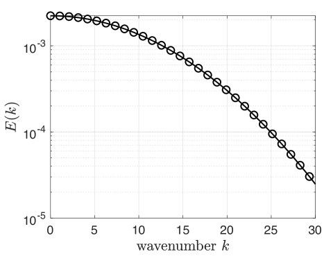
Figure 1: Fourier energy spectrum of the height perturbation initial condition $\phi^{(t)}(x)=\exp(-(10x)^{2})/20$. For wavenumbers $k>30$ the spectral energy densities are less than 1% of their maximum values which suggests taking $k_{max}=30$ is a reasonable approximation of the support of this particular initial condition in the Fourier space, cf. (24). This means that observation points with separations $\Delta x<\pi/30\lessapprox 0.1$ should satisfy the sufficient condition for convergence given in (26).

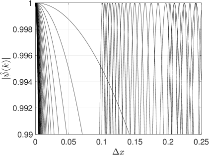
(a) $N_{\text{obs}}=2$, $\Delta k=1.$

(b) $N_{\text{obs}}=2$, $\Delta k=0.075.$

(c) $N_{\text{obs}}=4$, $\Delta k=1.$

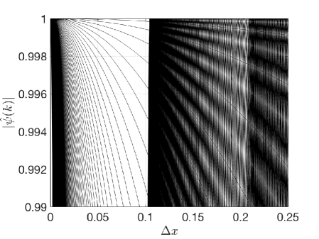
(d) $N_{\text{obs}}=4$, $\Delta k=0.075.$

(e) $N_{\text{obs}}=100$, $\Delta k=1.$

(f) $N_{\text{obs}}=100$, $\Delta k=0.075.$

Figure 2: Convergence properties of the gradient approach (23) for varying numbers of observation points $N_{\text{obs}}$ when the real line is discretized in wavenumber space with resolution $\Delta k$. Where $|\widehat{\psi}(k)|=1$, cf. (26), the assimilation does not converge to the correct initial data and when $|\widehat{\psi}(k)|$ is close to 1 we expect convergence to be slow. A clear transition between convergence to the correct and incorrect initial data is evident at $\Delta x=\pi/k_{\text{max}}$ (where $k_{\text{max}}=30$ fully resolves the initial condtion, Figure 1). Note that in this case the continuous problem converges for all $0<\Delta x<0.1$. In all cases the maximum wavenumber $k_{\text{max}}=30$ to fully resolve the exact initial condition (see figure 1). We see that, when $\Delta x<\pi/k_{\text{max}}$, the convergence increases with increasing number of observation points and also with coarser discretizations of the real line.

In the next section we present computational examples illustrating how these properties affect the accuracy and efficiency of the gradient-based solution of the data assimilation problem for the wave equation both in the linear and nonlinear regime.

5 Numerical solution of the data assimilation problem

Before presenting our computational results we briefly describe the numerical approach. While in the linear setting both the direct and adjoint problem (2) and (12) can be solved analytically, cf. Section 3, for ease of comparison with the nonlinear case these problems are solved numerically.

5.1 Numerical Methods

In order to simplify the numerical solution of the PDE problems, the unbounded spatial domain is replaced with a large periodic domain $[-L,L]$, where $L=3$ is chosen big enough to ensure that in combination with the observation time $T=2$ there are no boundary effects (i.e. the waves never get close to the domain boundary during the time window $[0,T]$). Both the forward and backward (adjoint) equations are discretized in space using a standard second-order finite-difference/finite-volume method on an evenly spaced staggered grid with $N=1024$ points. The height perturbation and velocity variables $\eta(x,t)$ and $u(x,t)$ are represented at the cell centres and at the cell boundaries, respectively. The resulting system of ordinary differential equations is integrated in time using a third-order strong stability preserving Runge–Kutta method [21]. Consistency of adjoint-based gradient evaluations in the linear and nonlinear setting was carefully checked by evaluating the directional derivative $\mathcal{J}^{\prime}(\phi;\phi^{\prime})$ using formulas (10)–(11) and comparing the results with a finite-difference approximation of $\mathcal{J}^{\prime}(\phi;\phi^{\prime})$ [13]. In the gradient-based optimization algorithm (9) the line-minimization problem (14) is solved using the MATLAB function fminunc.

5.2 Computational Results

In this section we present computational results illustrating the effect of the observability criterion introduced in Section 4 on the accuracy and efficiency of the gradient-based solution of the data assimilation problem.

In all cases the true initial condition for the height variable $\eta(x,0)$ has the form

$${\phi^{(t)}(x)}=\frac{1}{20}\exp^{-(10x)^{2}}$$

and is approximately supported on the interval $[-0.3,0.3]$ in physical space and the interval $[-30,30]$ in Fourier space, see figure 1 (the initial condition for the velocity variable $u(x,0)$ is zero, cf. (1c) and (2c)). We note that the choice of the support in Fourier space coincides with the value of $k_{\text{max}}$ used in Section 4. Such localized initial conditions are typical for the problem of tsunami waves propagation. We emphasize that the support of the initial condition $\phi^{(t)}(x)$ in physical space is ten times smaller than the size of the computational domain.

The true initial condition $\phi^{(t)}$ is used in conjunction with the forward model (1) or (2) and the observation operator defined in (4) to generate the observations $y^{(o)}_{j}(t)$, $j=1,\dots,N_{\text{obs}}$ used in the data assimilation problem (note that in our computations the observations are generated using the same model as the forward equations; SWE in both cases). In all cases we take a zero initial guess $\phi^{(0)}(x)=0$ to initialize the gradient iterations (9). Figure 3 shows the right-going parts of the linear and nonlinear SWE solutions at the observation time $T=2$. Both solutions are effectively zero at the boundary of the truncated computational domain ($L=3$) at this time. Recall that for the linear SWE the solution is simply a translated copy of the initial condition scaled by one half.

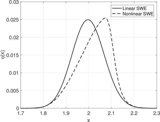
Figure 3: Right-going part of the linear and nonlinear SWE solutions at the observation time $T=2$. Note the significant difference between the two solutions.

The large computational domain and relatively short observation time ensure that the artificial (periodic) boundary conditions do not affect the solution (i.e. the domain remains effectively infinite). Therefore, choosing all observation points in the region $x>0$ means that they measure only the right-going part of the SWE wave solution and do not capture any information about the left-going part of the solution, as is typical for the case of tsunami observations.

Next, we present results for the convergence of the cost functional and of the $L^{2}$ error in the reconstructed initial conditions for both the linear and nonlinear SWE cases for different numbers of observations. It is important to remember that we minimize the cost functional ((6)), which is the $L^{2}$ norm of the difference between the observations and model integrated over the observation time, rather than the initial condition itself. We stress that, as demonstrated in Section 4, the assimilation algorithm will not necessarily converge for all choices of observation points.

Taking Theorem 26 and Figure 1 as guides, we compare a case where the sufficient condition for convergence is satisfied ($\Delta x={0.09}$) with a case where it is not ($\Delta x=0.375$). In both cases the algorithm is stopped after 1000 iterations. Figure 4 confirms that when the sufficient condition is satisfied, the algorithm converges for different numbers of observation points $N_{\text{obs}}>1$. A small value of the cost functional indeed corresponds to a small error in the reconstructed initial condition. The rate of convergence increases with the number of observation points, consistent with the observation that $|\widehat{\psi}(k)|$ is further from one as the number of observation points increases (see Figure 2(a, c, e)). Interestingly, taking only two observation points produces much worse results than three or more observation points. This suggests that in practical applications at least three observation points should be taken. Note that the linear and nonlinear SWE data assimilation problems exhibit similar behaviour, although the error for the nonlinear case is lower than for the linear case for four or more observation points. We have checked that these results are essentially identical for the case of an isolated bathymetry feature, $\beta(x)=\exp(-10(x-3/2)^{2})/10$ where the total mean depth is $1-\beta(x)$ (results not shown).

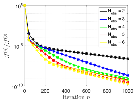
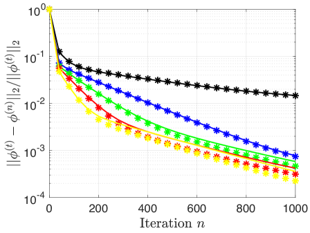
Figure 4: Convergence of (a) cost function $\mathcal{J}^{(n)}$ and (b) the reconstruction error $\|\phi^{(t)}-\phi^{(n)}\|_{L^{2}({\mathbb{R}})}$ as functions of iteration $n$ for different numbers of observation points for the linear (lines) and nonlinear (symbols) SWE when the first observation point is at $x=0.2$ and the observation points have uniform spacing $\Delta x=0.09$. Note that both the cost function and reconstruction error converge for all $N_{obs}$, although the rate of convergence increases with more observation points. The results for the linear and nonlinear SWE are similar.

In contrast, when the sufficient condition for convergence (26) is not satisfied, the algorithm fails to converge to the correct initial condition, or converges very slowly. Figure 5 shows convergence of the cost functional and error in the reconstructed initial condition with uniform spacing $\Delta x=0.375$. In this case, the error in the reconstructed initial condition is not reduced significantly for any number of observation points. The cost functional is reduced by five to seven orders of magnitude, although convergence is extremely slow after the first iteration. In contrast to the previous case, the cost functional is much larger for the nonlinear SWE assimilation, except for the case of two observation points.

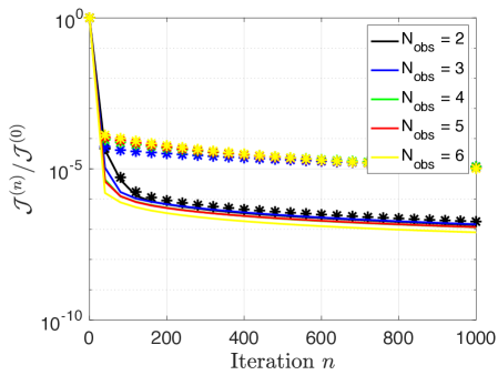
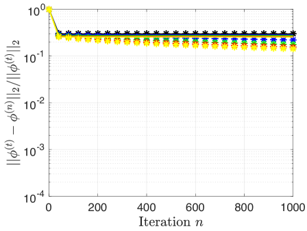
Figure 5: Convergence of (a) cost function $\mathcal{J}^{(n)}$ and (b) the reconstruction error $\|\phi^{(t)}-\phi^{(n)}\|_{L^{2}({\mathbb{R}})}$ as functions of iteration $n$ for different numbers of observation points for the linear (lines) and nonlinear (symbols) SWE when the first observation point is at $x=0.2$ and the observation points have regular spacing $\Delta x=0.375$. In this case $\Delta x$ does not satisfy the sufficient condition for convergence (26) and the reconstructed initial condition fails to converge to the correct initial condition $\phi^{(t)}$. Note that the different data sets overlap since there is little dependence on the number of observations points in this case where the initial conditions cannot be recovered.

Figure 6 compares the true initial condition $\phi^{(t)}$ and reconstructed initial conditions after $n=1000$ iterations $\phi^{(n)}\approx\phi^{(b)}$ for different spacings of observation points. In the first case, shown in Figure 6 (a), the sufficient condition for convergence to the true initial condition is satisfied and the initial condition is reconstructed exactly. In the second case, shown in Figure 6 (b), the sufficient condition is not satisfied and the reconstructed initial condition involves spurious oscillations spread throughout the computational domain, in addition to an approximation to the true Gaussian initial conditions (with a reduced magnitude).

Figure 6(c) shows that in the linear SWE case most of the error in the reconstructed initial condition is due to inaccuracies at wavenumbers $k=n\pi/\Delta x$, $n=1,2,3,4$ corresponding to the spacing of the observation points. Comparing the Fourier spectra shown in Figures 6 (c) and (d) indicates that results obtained with the linear and nonlinear models are much closer for $N_{\text{obs}}=2$ observation points than for four observation points. For $N_{\text{obs}}=4$ errors are smaller in the nonlinear SWE case, but occur at the same wavenumbers as in the linear SWE case. This observation is confirmed in Figure 7 in which lower errors are also evident for the nonlinear case at all spacings for four observation points. Finally, Figures 6(e) and (f) show similar results for the larger spacing $\Delta x=0.48$. The errors in the Fourier spectrum also occur at wavenumbers $k=n\pi/\Delta x$, confirming our analysis.

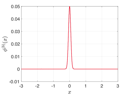
(a) $\Delta x=0.09$, $N_{\text{obs}}=4$.

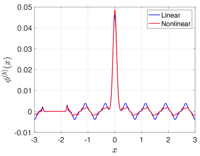
(b) $\Delta x=0.375$, $N_{\text{obs}}=4$.

(c) $\Delta x=0.375$, $N_{\text{obs}}=4$.

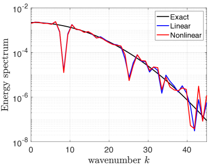
(d) $\Delta x=0.375$, $N_{\text{obs}}=2$.

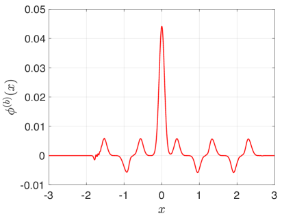
(e) $\Delta x=0.48$, $N_{\text{obs}}=2$.

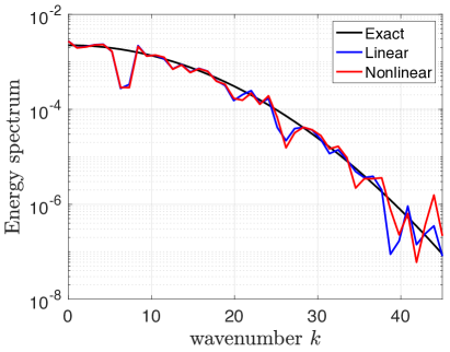
(f) $\Delta x=0.48$, $N_{\text{obs}}=2$.

Figure 6: Comparison of reconstructed initial conditions $\phi^{(b)}$ in physical and Fourier space for cases satisfying and not satisfying the sufficient condition  (26) for convergence to the true initial data $\phi^{(t)}$. (a) Spacing $\Delta x=0.09$ satisfying the sufficient condition, $N_{\text{obs}}=4$ The initial conditions $\phi^{(b)}$ reconstructed based on the linear and nonlinear models are both indistinguishable from the exact initial condition $\phi^{(t)}$. (b) Spacing $\Delta x=0.375$ not satisfying the condition for convergence, $N_{\text{obs}}=4$. The reconstructions based on the linear and nonlinear equations converge to different incorrect initial conditions. (c) Fourier spectra of (b) compared with the spectrum $\widehat{\phi}^{(t)}$ of the true initial condition. (d) As for (c), but with $N_{\text{obs}}=2$. (e) Spacing $\Delta x=0.48$ not satisfying the condition for convergence, $N_{\text{obs}}=2$. The reconstructions based on the linear and nonlinear equations both converge to the same incorrect initial conditions. (f) Fourier spectra of (e) compared with the spectrum $\widehat{\phi}^{(t)}$ of the true initial condition. The errors in the cases when convergence occurs to incorrect initial data are highly localized in Fourier space.

Finally, we examine how the error in the reconstructed initial condition $\phi^{(b)}$ changes as the uniform spacing $\Delta x$ between observation points varies between 0.0234 ($4h$, where $h$ is the computational grid spacing) and 0.5 for two and four observation points. Figure 7 confirms that the numerical results for the linear and nonlinear SWE data assimilations are qualitatively consistent in three ways with the analysis in Section 4, in particular, with the behavior of the function $|\widehat{\psi}(k)|$ shown in Figure 2.

First, when $\Delta x>0.2$, the error generally increases with increasing $\Delta x$. Secondly, the error also increases as $\Delta x\rightarrow 0$. Thirdly, the error is “spiky” for spacings $\Delta x>0.1$ due to the existence of a discrete set of wavenumbers where $|\widehat{\psi}(k)|=1$. The spikes are not visible in the case of two observation points since the peaks in $|\widehat{\psi}(k)|$ are very broad in this case (cf. Figures 2 (a) and (c)). The error is significantly lower at all spacings for the nonlinear SWE with $N_{\text{obs}}=4$, while the linear and nonlinear SWE results are very similar for two observation points.

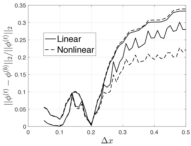
Figure 7: Error in the reconstructed initial condition $\phi^{(b)}$ as a function of spacing between observation points $\Delta x$ for $N_{\text{obs}}=2$ (upper curves) and $N_{\text{obs}}=4$ (lower curves) after 1000 iterations. Note that the oscillations in the reconstruction error are similar to the oscillations in the function $|\widehat{\psi}(k)|$ determining the convergence rate of the assimilation iterations shown in Figure 2.

6 Conclusions

This paper considers the problem of estimating the initial conditions for the one-dimensional SWE from wave height observations. We consider initial conditions with compact support and observations only to the right side of this support (so only the right-going wave is observed). This models the case of reconstructing the initial conditions for a tsunami wave where observations typically do not capture the total energy of the wave (which is the strict condition for observability with one observation point [31]). It is not clear a priori that the wave is observable under these conditions, even with multiple observation points.

This data assimilation problem is framed as PDE-constrained optimization in which a least-squares error functional is minimized with respect to the initial condition. Optimal reconstructions are computed with a gradient-based approach in which the cost functional gradients are evaluated based on solutions of adjoint equations. While in operational practice a “discretize-then-differentiate” approach is often adopted, in the present study we followed the “optimize-then-discretize” paradigm as it allowed us to derive a sufficient condition for the convergence of iterations to the true initial condition in the linear setting. Derivation and analysis of this condition, which is easy to verify, are the key contributions of this study.

The linear assimilation equations can be solved analytically, giving the exact expression for the gradient of the cost functional. Theorem 26 provides a sufficient condition for the existence of a unique fixed point corresponding to convergence to the true initial conditions. It turns out that the algorithm cannot converge at all for the case of a single observation point: at least two observation points must be used. However, the algorithm may also fail to converge to the true initial conditions even with multiple observation points. A sufficient condition for the existence of a unique fixed point is that at least one pair of observation points is closer than $\lambda_{\text{min}}/2$, where $\lambda_{\text{min}}$ is the minimum length scale of the true initial conditions. Note that $\lambda_{\text{min}}/2$ is the Nyquist frequency associated to the initial conditions. These results also apply to the linear wave equation.

Furthermore, the analytical results suggest that in the discrete case the rate of convergence increases with increasing numbers of observation points. This is confirmed by our numerical results. Interestingly, when the real line is discretized (rather than represented continuously) there are many observation point spacings larger than the critical spacing $\Delta x=\pi/k_{\text{max}}$ that may still converge to the correct initial data since the “bad” spacings are represented only by a discrete set of values (this set, however, becomes increasingly dense as the resolution is refined, i.e., as $\Delta k\rightarrow 0$). It is therefore possible, especially with low-resolution discretizations, that with a “lucky” choice of $\Delta x>\pi/k_{\text{max}}$ one may still recover the initial conditions with widely spaced observation points.

We have assumed that the observations are continuous in time. This is a realistic assumption for tsunami monitoring, and is natural for the continuous infinite-dimensional PDE-based data assimilation problem that we consider. In the case of discrete observations in time and wave speed $c$ it should be sufficient to sample the sea surface height at a frequency $f>c/(\lambda_{\text{min}})$ in order to capture the smallest scales of the wave.

Finally, we verify the performance of the data assimilation algorithm and the mathematical analysis for the case of a Gaussian initial condition with zero initial guess. The algorithm converges to the true initial condition for both the linear and nonlinear SWE provided there are at least two observation points and the points are sufficiently close together (as determined by the theorem). The rate of convergence increases with the number of observation points, and at least three points are needed for practically useful results. Relative $L^{2}$ errors in the reconstructed initial conditions of $O(10^{-2})$ are achieved in about 100 iterations and errors of $O(10^{-4})$ are achieved in 500–1000 iterations for six observation points. These results are essentially identical for the case of an isolated bathymetry feature, $\beta(x)=\exp(-10(x-3/2)^{2})/10$ where the total mean depth is $1-\beta(x)$.

We also confirmed that if the observation points are too widely spaced (so the sufficient condition is not satisfied) the algorithm converges to the wrong initial condition, for both linear and nonlinear SWE. The error is due to underestimating the energy at discrete wavenumbers $k=n\pi/\Delta x$, $n=1,2,3,\ldots$, where $\Delta x$ is the spacing between the observation points. Interestingly, this failure to converge to the true initial condition cannot be deduced from the behaviour of the cost functional which decreases to small values.

In addition to the simple gradient descent algorithm, we also solved the minimization problem (7) using two commonly used nonlinear conjugate gradient methods: Fletcher–Reeves and Polak-Ribiére. The results were consistent with the gradient descent method although, as expected, convergence was usually faster. Importantly, the conjugate gradient method did not modify the conditions for convergence to the true initial conditions, i.e. (26) (see Figure 5).

Although this one-dimensional case is not physically realistic, it allows for careful investigation of the potential and limitations of variational data assimilation for the tsunami problem where only a relatively small number of sparsely distributed observations are possible. More specifically, it makes it possible to identify sufficient conditions for convergence to the true initial condition that should provide guidance for the two-dimensional problem. In particular, the Nyquist-like condition on the spacing of observation points should carry over to the 2D case. Importantly, the numerical results have confirmed that the nonlinear problem behaves very similarly to the linear problem we solved exactly.

As a next step, we plan to investigate to what extent the results reported here generalize to the SWE on 2D planar domains, or to a global ocean model [12]. Mathematical analysis in such settings is more complicated due to the geometry of the problem, although probably possible for the linearized equations. A related question concerns using data assimilation to infer bathymetry information from sea surface height observations. Cobelli et al. [4] recently investigated the related problem of determining the shape of a localized movement of the seafloor from surface observations. Bathymetry, together with the initial conditions, are the two major factors affecting the accuracy of tsunami forecasting and available bathymetry data is often incomplete or of insufficient resolution.

Finally, we also intend to investigate optimal placement of observation points in the two-dimensional case including bathymetry effects. As an important enabler for these efforts, our dynamically adaptive wavelet method for the two-dimensional SWE on the sphere [12] opens up the possibility of adapting the computational grid to improve the accuracy of the assimilation.

References

- [1] A, L., Morales-Hernandez M, B.J., P, B., P., G.N.: Calibration of the 1d shallow water equations: a comparison of Monte Carlo and gradient-based optimization methods. J. Hydroinformatics (2017)
- [2] Bélanger, E., Vincent, A., Fortin, A.: Data assimilation (4d-var) for shallow-water flow: The case of the Chicoutimi river. Visual Geosciences 8(1), 1–17 (2003).
- [3] Berger, M.S.: Nonlinearity and Functional Analysis. Academic Press (1977)
- [4] Cobelli, P.J., Petitjeans, P., Maurel, A., Pagneux, V.: Determination of the bottom deformation from space- and time-resolved water wave measurements. J. Fluid Mech. 835, 301–326 (2017).
- [5] Coron, J.M.: Control and Nonlinearity. American Mathematical Society (2007)
- [6] Engl, H., Hanke, M., Neubauer, A.: Regularization of Inverse Problems. Kluver, Dordrecht (1996)
- [7] Gunzburger, M.D.: Perspectives in Flow Control and Optimization. SIAM (2003)
- [8] Guo, L., Wang, Z.: Exact boundary observability for nonautonomous quasilinear wave equations. Journal of Mathematical Analysis and Applications 364(1), 41–50 (2010).
- [9] Ide, K., Courtier, P., Ghil, M., Lorenc, A.: Unified notation for data assimilation: operational, sequential and variational. J. Meteorol. Soc. Jpn. 75, 181–189 (1997)
- [10] John, F.: Partial differential equations. Springer (1982)
- [11] Kalnay, E.: Atmospheric Modeling, Data Assimilation and Predictability. Cambridge University Press (2003)
- [12] Kevlahan, N.K.R., Dubos, T., Aechtner, M.: Adaptive wavelet simulation of global ocean dynamics using a new Brinkman volume penalization. Geoscientific Model Development 8(12), 3891–3909 (2015).
- [13] Khan, R.: A Data Assimilation Scheme for the One-dimensional Shallow Water Equations. Master’s thesis, McMaster University (2016)
- [14] Li, T., Li, D.: Exact boundary observability for 1-D quasilinear wave equations. Mathematical Methods in the Applied Sciences 29(13), 1543–1553 (2006).
- [15] Maeda, T., Obara, K., Shinohara, M., Kanazawa, T., Uehira, K.: Successive estimation of a tsunami wavefield without earthquake source data: A data assimilation approach toward real-time tsunami forecasting. Geophysical Research Letters 42(19), 7923–7932 (2015).
- [16] Nocedal, J., Wright, S.: Numerical Optimization. Springer (2002)
- [17] Okada, Y.: Surface deformation due to shear and tensile faults in a half-space. Bull. Seism. Soc. Amer. 75, 1135–1154 (1985)
- [18] Pires, C., Miranda, P.M.A.: Tsunami waveform inversion by adjoint methods. Journal of Geophysical Research: Oceans 106(C9), 19773–19796 (2001).
- [19] Protas, B., Bewley, T., Hagen, G.: A Comprehensive Framework for the Regularization of Adjoint Analysis in Multiscale PDE Systems. J. Comp. Phys. 195, 49–89 (2004)
- [20] R, S., A, S., M., N.I.: Pod/deim reduced-order strategies for efficient four dimensional variational data assimilation. J. Comp. Physics 295, 569–595 (2015)
- [21] Spiteri, R., Ruuth, S.: A new class of optimal high-order strong-stability-preserving time discretization methods. SIAM J. Numer. Anal. 40, 469–491 (2002)
- [22] Stengel, R.F.: Optimal Control and Estimation. Dover (1994)
- [23] Steward, J.L., Navon, I.M., Zupanski, M., Karmitsa, N.: Impact of non-smooth observation operators on variational and sequential data assimilation for a limited-area shallow-water equation model. QUARTERLY JOURNAL OF THE ROYAL METEOROLOGICAL SOCIETY 138(663, B), 323–339 (2012).
- [24] Tarantola, A.: Inverse Problem Theory and Methods for Model Parameter Estimation. SIAM (2005)
- [25] Tirupathi, S., Tchrakian, T.T., Zhuk, S., McKenna, S.: Shock capturing data assimilation algorithm for 1d shallow water equations. Advances in Water Resources 88, 198 – 210 (2016).
- [26] Titov, V., Rabinovich, A., Mofjeld, H., Thomson, R., González, F.: The global reach of the 26 December 2004 Sumatra tsunami. Science 309, 2045–2048 (2005)
- [27] Vlasenko, A., Korn, P., Riehme, J., Naumann, U.: Estimation of data assimilation error: A shallow-water model study. Monthly Weather Review 142(7), 2502–2520 (2014).
- [28] Żabczyk, J.: Mathematical Control Theory. An Introduction. Birkhäuser (1995)
- [29] Zhu, K., Navon, I.M., Zou, X.: Variational data assimilation with a variable resolution finite-element shallow-water equations model. Monthly Weather Review 122(5), 946–965 (1994).
- [30] Zou, X., Navon, I., Dimet, F.L.: Incomplete observations and control of gravity waves in variational data assimilation. Tellus A: Dynamic Meteorology and Oceanography 44(4), 273–296 (1992)
- [31] Zuazua, E.: Propagation, observation, and control of waves approximated by finite difference methods. SIAM Review 47(2), 197–243 (2005)