Neural Tensor Factorization

Abstract.

Neural collaborative filtering (NCF) (He et al., 2017) and recurrent recommender systems (RRN) (Wu et al., 2017) have been successful in modeling user-item relational data. However, they are also limited in their assumption of static or sequential modeling of relational data as they do not account for evolving users’ preference over time as well as changes in the underlying factors that drive the change in user-item relationship over time. We address these limitations by proposing a Neural network based Tensor Factorization (NTF) model for predictive tasks on dynamic relational data. The NTF model generalizes conventional tensor factorization from two perspectives: First, it leverages the long short-term memory architecture to characterize the multi-dimensional temporal interactions on relational data. Second, it incorporates the multi-layer perceptron structure for learning the non-linearities between different latent factors. Our extensive experiments demonstrate the significant improvement in rating prediction and link prediction on dynamic relational data by our NTF model over both neural network based factorization models and other traditional methods.

1. Introduction

Learning from relational data (e.g., the user-item interactions on Netflix) has benefited many real-world services and applications, such as rating prediction and item recommendation on online platforms. A significant line of research has shown that latent factor models, in particular factorization based techniques, offer state-of-the-art results for learning tasks on relational data (Koren, 2008; Mnih and Salakhutdinov, 2008; Ma et al., 2008). In addition, as the main framework of the winning solution of the Netflix Prize, matrix factorization (MF) has demonstrated its power on industrial-grade applications (Koren et al., 2009), further attracting much effort in generalizing its predictive abilities.

One direction of these efforts has been devoted to extending a two-dimensional matrix, representative of interactions between users and items, into a three-dimensional tensor for incorporating the time information. Subsequently, the tensor factorization (TF) technique can be employed to project users and items into a latent space with the encoding of time (Kolda and Bader, 2009; Bhargava et al., 2015). However, conventional TF assumes the independence between two consecutive time slots, leaving it infeasible to make predictions for the next time slot. Further, it is also incapable of capturing the temporal patterns that are themselves time-evolving, such as (i) the fast-changing item perception, for example, individuals’ impression to a movie may be dynamically affected by its winning of some movie awards. and (ii) the evolution of users’ preferences, i.e., user’s tastes may change over time.

Recently, another attempt—recurrent recommender networks (RRN)—was made to integrate a recurrent neural network with factorization models for modeling the sequence dependencies between users’ behavioral trajectories (Wu et al., 2017). However, RRN achieves this by setting a fixed length of items’ historical ratings, ignoring the time interval between two consecutive ratings. Consequently, these fixed-length (e.g., $k$) rating sequences may cover various time-frames for different items. This is a limitation of RRN. For example, a popular movie may only take one hour to receive $k$ ratings, while a cult movie may need days to collect the same count of ratings. Additionally, both RRN and conventional TF models utilize dot product to make rating predictions, missing the potential to model the nonlinearities between latent factors.

To address these challenges and limitations, we develop a Neural network based Tensor Factorization model (NTF). In general, the NTF takes a three-way tensor (i.e., user-item-time) as input and learns the latent embeddings (commonly referred to as factors in TF) for each dimension of the tensor. Specifically, NTF integrates the long short-term memory (LSTM) network with tensor factorization. The LSTM module is used to adaptively capture the dependencies among multi-dimensional interactions based on the learned representations for each time slot. Furthermore, instead of using dot product between learned representations to make rating predictions, NTF concatenates the inherent factors together and feeds them into a Multilayer Perceptron (MLP) architecture. As such, the learned representations encode the non-linear interactions between different dimensions.

In addition to the aforementioned differences with RRN, our NTF also differs from it with respect to the input to the LSTM module. To predict the next rating, the input to RRN’s LSTM is the previous rating sequence with a fixed length, while the LSTM module of NTF takes the representation vectors from previous time slots. Furthermore, NTF is different from the recent work on neural collaborative filtering (NCF) (He et al., 2017) and collaborative deep learning (CDL) (Wang et al., 2015), whereas they infers the users’ and items’ latent embeddings under a static scenario. Additionally, different from CDL, NTF does not need auxiliary information and domain knowledge to determine the effectiveness of features. The advantage of the NTF  model lies in its complete utilization of each dimension of the relational data.

To sum up, the main contributions of this paper include:

• To the best of our knowledge, we present the first model to generalize tensor factorization with deep neural networks, empowering it to model time-evolving multi-dimensional data. We call this NTF.

• We incorporate the multiple-layer perceptron architecture in NTF for modeling the non-linearities in relational data, eliminating the linear limitation of dot product used in conventional tensor factorization.

• We perform extensive experiments for the problems of rating prediction in the Netflix dataset and link prediction in the Github dataset, demonstrating the significant improvements over state-of-the-art baselines, such as RRN and NCF.

2. Problem Formulation and
Tensor Factorization (TF)

In this section, we present the notations and problem formulation. We also provide a quick review of the conventional Tensor Factorization (TF) model and discuss its limitations in modeling the temporal dynamics of relational data.

2.1. Problem Formulation

We consider a dynamic scenario wherein there exists evolving pair-wise relations between multiple types of entities (e.g., user, item, and time), such as Netflix users’ ratings to various movies on different days, and Github users’ repository forks during a month. To model the relationships among entities over time, we use a tensor to represent their time-evolving interactions.

In this work, we focus on the three-way tensor with a temporal dimension. Formally, we construct a tensor $\mathcal{X}\in\mathbb{R}^{I\times J\times K}$ denoting the first-order tensor of each dimension with a size of $I$, $J$ and $K$, respectively. We denote the entry in the tensor $\mathcal{X}$ as $x_{i,j,k}$ to represent the interactions among different dimensions which are indexed by $i$, $j$ and $k$, respectively. For example, in relational rating data, $x_{i,j,k}$ can represent: (i) the quantitative rating score of $i$-th user on $j$-th item in $k$-th time slot, and (ii) the binary interactions (links) between $i$-th and $j$-th nodes at time slot $k$.

Problem Formulation. Based on the above definitions, we use $x_{i,j,k}$ to represent the interactions among three dimensions in tensor $\mathcal{X}$ which are observed from relational data. The objective of this work is to learn a predictive model that can effectively infer the unknown values in $\mathcal{X}$ with the observed ones.

2.2. Conventional Tensor Factorization

The key idea of tensor factorization is learning connections among the observed values in a tensor in order to infer the missing ones. The most common mechanism of tensor factorization is CANDECOMP/PARAFAC (CP) (Carroll and Chang, 1970), which decomposes a tensor into multiple low-rank latent factor matrices representing each tensor-dimension. For example, movie rating dataset can be viewed as a tensor with $3$-dimensions: user, movie, and time. The latent factor matrices in this case, measure the latent factors of each dimension. The latent factors on user-dimension may be users’ genre or rating preferences, the factor matrix on movie-dimension may model the movie plot, starring information, and many other features, the time-dimension factors could be specific time related information such as holiday season or special events. With these three matrices, the ratings can be obtained by a simple dot product across the matrices. Following the convention in Representation Learning (RL) literature, in this work we will refer inherent factor vectors as lower-dimensional embedding or representation vectors interchangeably (Bengio et al., 2013).

Formally, TF factorizes a tensor into three different matrices $U\in\mathbb{R}^{I\times L}$, $I\in\mathbb{R}^{J\times L}$ and $T\in\mathbb{R}^{K\times L}$, where $L$ is the number of latent factors (indexed by $l$). We define the factorization of tensor $\mathcal{X}$ as:

(1) $$\mathcal{X}\approx\sum_{l=1}^{L}U_{:,l}\circ I_{:,l}\circ T_{:,l},$$

where $U_{:,l}$, $I_{:,l}$ and $T_{:,l}$ represents the $l$-th column of matrices $U$, $I$ and $T$ respectively. $\circ$ denotes the vector outer product. Each entry $x_{i,j,k}\in\mathcal{X}$ can be computed by the inner-product of three $L$-dimensional vectors as follows:

(2) $$\hat{x}_{i,j,k}\approx<U_{i},I_{j},T_{k}>\equiv\sum_{l=1}^{L}U_{i,l}I_{j,l}T_{k,l}.$$

The objective of tensor factorization is to learn $U$, $I$ and $T$ using maximum likelihood estimation. We further define $U_{i}$, $I_{j}$ and $T_{k}$ to index the row of $U\in\mathbb{R}^{I\times L}$, $I\in\mathbb{R}^{J\times L}$ and $T\in\mathbb{R}^{K\times L}$, respectively. After the model learns $U$, $I$, and $T$ from the observed $\mathcal{X}$, one can easily fill in the missing values in $\mathcal{X}$ using Eq. 2.

However, two significant limitations exist in conventional tensor factorization model: (i) it fails to capture temporal dynamics because the interaction prediction $\hat{x}_{i,j,k}$ only depends on current timeslot $T_{k,:}$; (ii) it is a linear model which cannot deal with complex non-linear interactions that exist in real-world relational data. In the present work we aim to explicitly incorporate temporal dynamics into tensor factorization frameworks and model the non-linear interactions across different latent factors.

3. Neural network based Tensor Factorization Framework

In this section, we present the Neural network based Tensor Factorization (NTF) framework, which is capable of learning implicit time-evolving interactions in relational data. We first introduce the general framework of NTF to elaborate the motivation of the model and then present details of NTF in the following subsections.

3.1. General Framework

Our NTF is a multi-layer representation learning model which pursues a full neural treatment of tensor factorization to explicitly model the time-evolving interactions between different dimensions. We include the model architecture in Figure 1 and present the pseudo code of NTF in Algorithm 1. The motivations of designing our model are listed as follows:

• To address the data sparsity challenge, in our raw time embedding layer, we transform the element from the first-order tensor of temporal dimension with one-hot encoding and then project them into embedding space. In this way, we can address the sparse tensor challenge by using the latent vectors to represent elements of temporal dimension instead of using hand-crafted features.

• To capture the complex temporal dynamics, with the generated embedding vectors as input, we utilize LSTM to encode the evolving interactions addressing the issues of long-term dependencies and vanishing gradients in recurrent neural networks (Jozefowicz et al., 2015). Note that there are other variants of gated recurrent neural networks, such as Gated Recurrent Unit (GRU) (Chung et al., 2015). LSTM and GRU models bear some resemblance in the architecture and often provides similar results (Chung et al., 2014). This work chooses LSTM as the encoder for the temporal dimension of the tensor because it is slightly more general compared to others (Wu et al., 2017). As a general tensor factorization framework, NTF is also flexible to integrate other variants of recurrent neural networks.

  

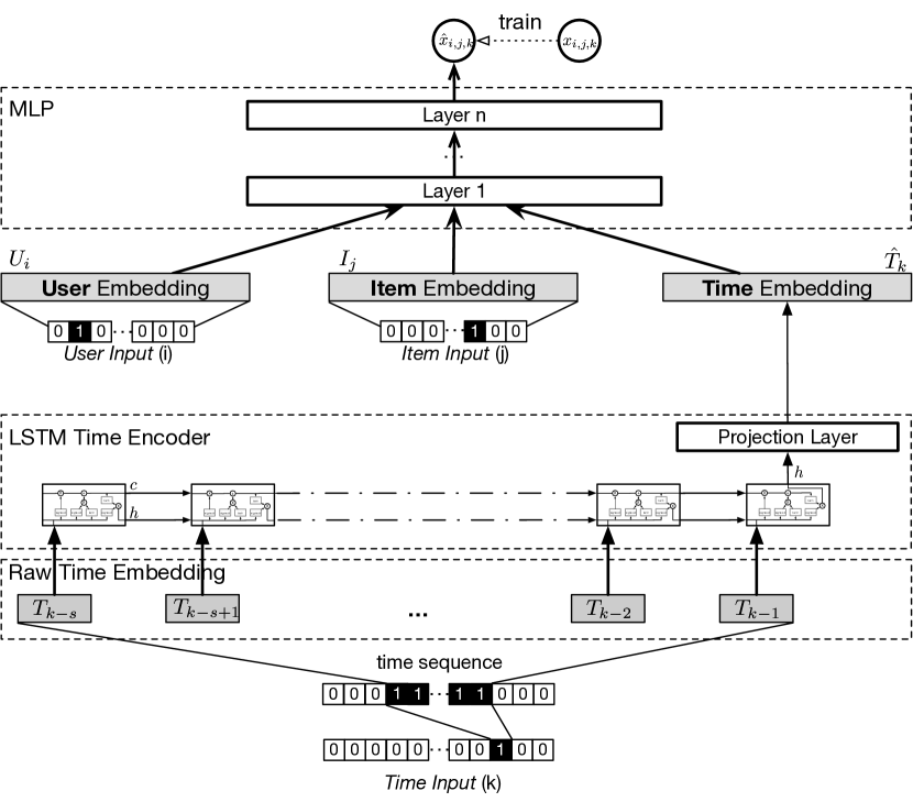
  Figure 1. The Neural network based Tensor Factorization (NTF) Framework.

• To model the non-linearity of multi-dimensional interactions, we decide to use a Multi-layer Perceptron (MLP) on top of the first two layers. Let us consider the generated tensor with user-item-time dimensions as an example. The projected temporal embedding vectors will be fed into a multi-layer neural architecture together with the embedding vectors of users and items. This enables NTF to incorporate the learned complex dependencies in the temporal dimension into the factorization process as constrains. By doing so, we can detect the implicit patterns of user-item-time interactions through each layer in the MLP framework and model the non-linear combinations of latent factors to make better predictions. Finally, the latent vectors will be mapped to quantitative values (i.e., $\hat{x}_{i,j,k}$) which represents future interactions across different dimensions.

1

2

3

4

5

6

7

Input: Tensor $\mathcal{X}$ $\in\mathbb{R}^{I\times J\times K}$, observed interaction set $\mathbf{X}$, sequence length $s$, and batch size $b_{\textsf{size}}$.

Paras : Embedding matrices $\textnormal{{$\mathbf{U}$}}\in\mathbb{R}^{I\times L}$, $\textnormal{{$\mathbf{I}$}}\in\mathbb{R}^{J\times L}$, $\textnormal{{$\mathbf{T}$}}\in\mathbb{R}^{K\times L}$, and other hidden parameters $\theta$.

8

9Initialize all parameters;

// Sample a minibatch of size $b_{\textsf{size}}$.

10 foreach $\textnormal{{$\mathsf{T_{batch}}$}}=\textnormal{{sample}}(\textnormal{{$\mathbf{X}$}},\textnormal{{$b_{\textsf{size}}$}})$ do

11       foreach $\langle i,j,k\rangle\in\textnormal{{$\mathsf{T_{batch}}$}}$ do

             /* Gather embeddings for all dimensions. */

12             $\textnormal{{U}}_{i}=\textnormal{{$\mathbf{U}$}}[i,:]$, $\textnormal{{I}}_{j}=\textnormal{{$\mathbf{I}$}}[j,:]$;

13            

            $c=c_{0},h=h_{0}$;

              // init. hidden states

14             for $\textnormal{{t}}\leftarrow(k-\textnormal{{$s$}})$ to $(k-1)$ do

                   $c,h=\textnormal{{LSTM}}(\textnormal{{$\mathbf{T}$}}[\textnormal{{t}},:],c,h)$;

                    // according to Eq.3

15                  

16             end for

            $\textnormal{{$\hat{\mathbf{T}}$}}_{k}=\textnormal{{Projection}}(h)$;

              // encoded time embedding

17            

            $\textnormal{{$\hat{x}_{i,j,k}$}}=\textnormal{{MLP}}([\textnormal{{U}}_{i};\textnormal{{I}}_{j};\textnormal{{$\hat{\mathbf{T}}$}}_{k}])$;

              // according to Eq.6

18             $\textnormal{{$x_{i,j,k}$}}=\textnormal{{$\mathcal{X}$}}[i,j,k]$;

19             update loss $\mathcal{L}$ w.r.t $\frac{1}{2}(\textnormal{{$x_{i,j,k}$}}-\textnormal{{$\hat{x}_{i,j,k}$}})^{2}$;

20            

21       end foreach

22      update all parameters w.r.t $\mathcal{L}$;

23      

24 end foreach

Algorithm 1 Training the NTF model.

3.2. Modeling Temporal Dynamics via LSTM

Recurrent Neural Network (RNN) has been widely used to address various challenges in time series analysis. However, two key limitations exist in the basic RNN. First, it is difficult to train due to the problem of gradient vanishing and exploding, since the gradient might approach zero (vanish) or diverge (explode) as it is propagated back through time steps during the training process. Second, it is incapable to model long-distance dependencies in sequence data. To obviate the above problems and make the architecture more effective, LSTM is introduced as a special kind of RNN to model long-term dependencies and addresses the vanishing gradient problem by developing a more complicated hidden unit. In particular, LSTM proposes to derive the vector representations of hidden states $h_{t}$ and $c_{t}$ for each time step $t$ as follows:

$$i_{t}= \sigma(W_{i}h_{t-1}+V_{i}x_{t}+b_{i})$$

$$o_{t}= \sigma(W_{o}h_{t-1}+V_{o}x_{t}+b_{o})$$

$$f_{t}= \sigma(W_{f}h_{t-1}+V_{f}x_{t}+b_{f})$$

$$\widetilde{c_{t}}= \phi(W_{c}h_{t-1}+V_{c}x_{t}+b_{c})$$

$$c_{t}= f_{t}\odot c_{t-1}+i_{t}\odot\widetilde{c_{t}}$$

(3) $$h_{t}= o_{t}\odot\phi(c_{t})$$

where $W_{*}\in\mathbb{R}^{d_{s}\times d_{s}}$ represents the transformation matrix from the previous state (i.e., $c_{t-1}$ and $h_{t-1}$) to LSTM cell and $V_{*}\in\mathbb{R}^{d_{x}\times d_{s}}$ are the transformation matrices from input to LSTM cell, where $d_{x}$ and $d_{s}$ denotes the dimension of input vectors and hidden states, respectively. Furthermore, $b_{*}\in\mathbb{R}^{d_{s}}$ is defined as a vector of bias term. $\sigma(\cdot)$ and $\phi(\cdot)$ represents the sigmoid and tanh function, respectively. The $\odot$ operator denotes the element-wise product. In Eq. 3, $i_{t}$, $o_{t}$, and $f_{t}$ represents input gate, output gate and forget gate, respectively. For simplicity, we denote Eq. 3 as $[c_{t},h_{t}]=\text{LSTM}(*,c_{t-1},h_{t-1})$ in the following subsections.

3.3. Fusion of LSTM and TF

In this subsection, we present how we fuse LSTM and TF under the NTF framework to model the time-evolving interactions across three dimensions $\mathbb{R}^{I}$, $\mathbb{R}^{J}$ and $\mathbb{R}^{K}$. In relational data, dynamic characteristics are observed across different time slots. In this work, we consider temporal factors affecting the interactions over time based on a global trend by assuming that the interactions between multi-dimensions evolve in a smooth way. In particular, to capture the temporal smoothness, we further assume that the embedding vectors of the temporal dimension depends on embedding vectors from previous $s$ time slots. In NTF, we predict the embedding vector in current time slot based on the embedding vectors from past $s$ time slots using LSTM.

To encode the evolving temporal hidden factors, our LSTM encoder generates embedding without using hand-crafted features (e.g., the day of a week). We formally define the hidden states $c_{t}$ and $h_{t}$ in encoding the contextual sequence as:

$$[c_{1},h_{1}]= \text{LSTM}(T_{k-s},c_{0},h_{0})$$

$$\cdots$$

(4) $$[c_{s-1},h_{s-1}]= \text{LSTM}(T_{k-1},c_{s-2},h_{s-2})$$

Using the last hidden state vector $h_{s-1}$, we can define the embedding vector $\hat{T}_{k}$ through Projection Layer as:

(5) $$\hat{T}_{k}= \phi_{n}(W_{T}h_{s-1}+b_{T})$$

where $W_{T}\in\mathbb{R}^{s\times L}$ is the projection matrix, $b\in\mathbb{R}^{L}$ is the projection bias. $\phi$ are activation functions that we define later.

Finally, the predictive value $\hat{x}_{i,j,k}$ could be derived by the dot product of $U_{i}$, $I_{j}$, $\hat{T}_{k}$ according to the conventional tensor factorization. With the increasing utilization of deep neural networks to handle complicated non-linearity in image and text data (Collobert et al., 2011; Rigamonti et al., 2011), it is intuitive to explore the non-linear interactions in relational data. To address this issue, we concatenate embedding vectors of $U_{i}$, $I_{j}$, $\hat{T}_{k}$ together and consider them as input to the Multi-Layer Perceptron (MLP) and output $\hat{x}_{i,j,k}$. In this way, we can address the limitation caused by the dot product in tensor factorization (as introduced in Section 2) with a neural network architecture to capture non-linear interactions by concatenating latent factors from the previous embedding layer. Formally, we present MLP as:

$$Z_{1}= \phi_{1}(W_{1}[U_{i};I_{j};\hat{T}_{k}]+b_{1})$$

$$\cdots$$

$$Z_{n}= \phi_{n}(W_{L}Z_{n-1}+b_{L})$$

(6) $$\hat{x}_{i,j,k}= W_{o}Z_{n}+b_{o}$$

where $n$ represents the number of hidden layers which is indexed by $l$ and ; represents the concatenate operation. For the $Z_{l}$ layer, $\phi_{l}$, $W_{l}$ and $b_{l}$ represent the activation function (e.g., $ReLU$ or $tanh$ function) of MLP layers, weight matrix and bias vector, respectively. We further specify the activation function as sigmoid (denoted as $\sigma$) to output the quantitative values representing multi-dimensional interactions. In the experiments, we investigate the effect of number of layers in MLP.

3.4. Learning Process

In this subsection, we first describe the learning process of our NTF framework. Then, we further utilize the advanced technique, i.e., batch normalization, to optimize the NTF.

3.4.1. The Objective Function.

As we introduced in the Section 2, our objective is to derive the value of $\hat{x}_{i,j,k}$ which denotes the interactions between $i$-th, $j$-th and $k$-th elements of first-order tensor $\mathbb{R}^{I}$, $\mathbb{R}^{J}$ and $\mathbb{R}^{K}$ in $\mathcal{X}$, respectively. We formally define our objective function in factorization procedure as follows:

(7) $$\operatorname*{argmin}_{U,I,T}\frac{1}{2}\sum_{(i,j,k)\in\mathbf{X}}(x_{i,j,k}-\hat{x}_{i,j,k})^{2}$$

where $\mathbf{X}$ denotes the set of observed interactions in tensor $\mathcal{X}$. The NTF can be learned by minimizing the above loss function between the observed interaction data and the factorization representation. The above optimization problem can be efficiently solved using a popular optimizer Adaptive Moment Estimation (Adam). The reasons to choose Adam are mainly two-folds: (i) it can automatically tune the learning rate during the training, and (ii) it often provides faster convergence compared with stochastic gradient descent algorithm.

3.4.2. Batch Normalization.

In the training process of neuron network models, their performances could be degraded by covariance shift (Shimodaira, 2000). To tackle this challenge, Batch Normalization (BN) has been proposed to normalize the input data from previous layer before sending it to the next layer as input (Ioffe and Szegedy, 2015). In NTF framework, we apply BN to reduce the internal covariance shift by transforming the input to zero mean/unit variance distributions in each mini-batch training. In NTF, we apply the BN to LSTM to avoid the deceleration in training process as:

(8) $$\widetilde{c_{t}}= \phi(BN(W_{c}h_{t-1}+V_{c}x_{t}+b_{c}))$$

where $BN(\cdot)$ stands for the batch normalization operation. BN is also applied to Projection Layer.

4. Evaluation

We demonstrate the effectiveness of NTF with two real-world applications on dynamic relational data, i.e., regression-rating prediction and classification-link prediction corresponding to predicting quantitative (rating scores) and binary (existence of links) interactions, respectively. In particular, we aim to answer the following questions:

• Q1: How does our NTF framework perform as compared to the state-of-the-art techniques in rating prediction task?
  

• Q2: How does our NTF framework work for link prediction task when competing with baselines?
  

• Q3: Does NTF consistently outperform other baselines in terms of prediction accuracy with respect to different time windows with different training and testing time period?
  

• Q4: How is the performance of NTF variants with different combinations of key components in the joint framework?
  

• Q5: How different hyper-parameter settings (e.g., embedding size and number of hidden layers) affect the performance of NTF?

4.1. Experimental Setup

4.1.1. Data

In our evaluation, we perform experiments on two types of dynamic relational datasets and corresponding tasks, namely: (i) rating prediction on Netflix movie rating data; (ii) link prediction on Github archive data.

Netflix Rating Data. This movie rating dataset, which was collected between Jan 2002 and Dec 2005, has been widely used in rating prediction evaluation (Xiong et al., 2010; Shih et al., 2016). In the Netflix dataset, users rate a movie using a 1 (worst) to 5 (best) scale, the given score is also associated with a rating date to denote when the rating was reported. We generate tensor $\mathcal{X}$ by associating each movie with the users who rated this movie on different months. In particular, if $i$-th user rated $j$-th movie on $k$-th month (the time slots we used for evaluation correspond to calendar months) in the dataset, the element $x_{i,j,k}$ is in the interaction set $\mathcal{X}$.

Github Archive Data. This dataset was collected from Github to record the fork actions of users on repositories. Specifically, forking a repository allows users to freely experiment with changes without affecting the original project. Note that for any repository a user can only fork it once. The collection lasts for $6$-month (Jan 2017 to Jun 2017) and the time information is provided. In this dataset, an edge (i,j,k) is generated when $i$-th user forks the $j$-th repository at time slot $k$ (the time slots we used for evaluation correspond to calendar weeks). We set the element $x_{i,j,k}$ in $\mathcal{X}$ tensor to 1 if edge $(i,j,k)$ exists in the dataset and 0 otherwise.

Table 1. The Statistics of Datasets

	# of Users	# of Items	# of Ratings	Time Span
Netflix	68,079	2,328	12,326,319	36 months
	# of Users	# of Projects	# of Fork	Time Span
Github	81,001	72,420	1,396,115	21 weeks

Table 1 summarizes the statistics of the above two datasets. To better understand the effectiveness of NTF in modeling temporal dynamics, we evaluate NTF on different time windows with different training and testing period. Additionally, to evaluate the ability of our NTF to model temporal dynamics with time-evolving interactions among data, we remove users and items in the testing data which are not included in the training data. Table 2 shows the details to summarize of the experimental settings by varying time windows.

Table 2. Different Netflix data splits used in rating prediction.

# of users	# of items	training size	validation size	testing size	training period	testing period
28,077	1,772	1,454,868	145,486	225,787	Jan 2003-Dec 2004	Jan 2004
32,637	1,862	1,910,235	191,023	247,956	Mar 2003-Feb 2004	Mar 2004
37,060	1,937	2,437,882	243,788	270,312	May 2003-Apr 2004	May 2004
40,922	1,986	2,941,755	294,175	288,037	Jul 2003-Jun 2004	Jul 2004
44,072	2,055	3,388,774	338,877	305,693	Sep 2003-Aug 2004	Sep 2004
47,480	2,126	3,869,204	386,920	357,878	Nov 2003-Oct 2004	Nov 2004

4.1.2. Baselines

Because rating prediction and link prediction are two different tasks and have different representative baselines. Here, we summarize the compared baselines of these two tasks separately. In addition, the reason to compare NTF with matrix factorization methods rather than tensor factorization schemes is mainly twofold: (1) it is difficult to apply tensor factorization with temporal dimension to make predictions due to the ignorance of temporal dependencies between time slots. (2) There is no duplicate interactions (i.e., ratings and links) existed between users and items in different time slots in both Netflix and Github datasets.

Rating Prediction and Inference. For the rating prediction, we consider three types of baselines: representative matrix factorization for recommendation systems, neural network based collaborative filtering methods for recommendations or predictive analytics, and variants of Recurrent Neural Network models for time series prediction.

• Probabilistic Matrix Factorization (PMF) (Mnih and Salakhutdinov, 2008): it is a probabilistic method for matrix factorization, which assigns a D-dimensional latent feature vector (following Gaussian distributions) for each user and item. The ratings are derived from the inner-product of corresponding latent features.

• Bayesian Probabilistic Matrix Factorization (BPMF) (Salakhutdinov and Mnih, 2008): extended from the PMF, BPMF learns the latent feature vector for each user and item by Monte Carlo Markov Chain method, which is able to address the overfitting issue.

• Bayesian Probabilistic Tensor Factorization (BPTF)  (Xiong et al., 2010): it is a bayesian probabilistic tensor factorization method for modeling evolving relational data.

• Temporal Deep Semantic Structured Model (TDSSM) (Song et al., 2016): this method is a temporal recommendation model which combines traditional feedforward networks (DSSM) with LSTM, to capture temporal dynamics of users’ interests.

• Recurrent Recommendation Networks (RRN) (Wu et al., 2017): it aims to predict future interactions between users and items by specifying two embedding vectors (stationary and dynamic) for both user and item. The dynamic embedding vectors are inferred with LSTM model based on historical ratings.

• Neural Collaborative Filtering (NCF) (He et al., 2017): it proposed a framework for collaborative filtering based on neural network architecture to model the interactions between users and items.

4.1.3. Evaluation Protocols

In our evaluation, we split the datasets into training, validation and test sets. We use the validation datasets to tune hyper-parameters and test datasets to evaluate the final performance of all compared algorithms.

• Rating Prediction. To evaluate the performance of all compared algorithms in predicting quantitative rating scores, we use Root Mean Square Error (RMSE) and Mean Absolute Error (MAE) which have been widely adopted in quantitative prediction tasks (He and Chua, 2017). Note that a lower RMSE and MAE score indicates better performance. The mathematical definitions of those metrics are presented as follows: $RMSE=\sqrt{\frac{1}{N}\sum_{(i,j,k)\in\mathbf{X}}(x_{i,j,k}-\hat{x}_{i,j,k})^{2}}$, $MAE=\frac{1}{N}\sum_{(i,j,k)\in\mathbf{X}}|x_{i,j,k}-\hat{x}_{i,j,k}|$, where $N$ denotes the number of observed elements in tensor $\mathcal{X}$, $x_{i,j,k}$ and $\hat{x}_{i,j,k}$ represents the actual rating score and estimated rating score, respectively.

• Link Prediction. To validate the performance of each method in predicting the existences of links, Precision, Recall, F1-score and AUC are used as evaluation metrics (Scellato et al., 2011).

4.1.4. Reproducibility

We summarize the parameter settings of NTF and experiments in Table 3. In addition, we vary each of key parameters in NTF and fix others to examine the parameter sensitivity. We implemented our framework based on TensorFlow and chose Adam (Kingma and Ba, 2014) as our optimizer to learn the model parameters. For all neural network baselines (i.e., NCF, RRN and TDSSM), we use the same parameters listed in Table 3.

Table 3. Parameter Settings

Parameter	Value	Parameter	Value
Hidden State Dimension	32	Embedding size	32
# of Time Steps	5	# of Hidden Layers	6
BN scale parameter	0.99	BN shift parameter	0.001
Batch size	256	Learning rate	0.001

Table 4. Baseline Summary

Method PMF BPMF AA AP TDSSM RRN NCF BPTF NTF Rating Prediction ✓ ✓ ✓ ✓ ✓ ✓ Rating Inference ✓ ✓ ✓ ✓ ✓ ✓ ✓ Link Prediction ✓ ✓ ✓ ✓ ✓ ✓

Link Prediction. In addition to the above NCF, BPMF and PMF algorithms which have been applied to solve link prediction problem, we consider other two traditional link prediction baselines to compare the performance of NTF in predicting future binary interactions (i.e., links) among users.

• Preferential Attachment (PA) (Liben-Nowell and Kleinberg, 2007): PA assumes new connections are more likely to form between well-connected nodes.

• Adamic Adar (AA) (Adamic and Adar, 2003): AA smoothes the common neighbor method using neighbors’ node degree.

• PMF, BPMF, and NCF: as introduced above.

• TDSSM and RRN: both methods require the historical sequences of items and users. However, the sequences can not be generated from the Github dataset due to the following two reasons: First, the unobserved interactions may be either negative or positive cases; Second, if we take all unobserved cases as negative, it is also difficult to locate them to specific time slots.

For all embedding based and recurrent neural network based baselines, we use the same parameters as NTF which are listed in Table 3.

4.1.5. Variants of NTF

In addition to comparing NTF with existing approaches, we are also interested in discovering the best way to model non-linear multi-dimensional interactions among different embeddings in the proposed NTF framework. Namely, we aim to answer the following two questions: (1) does the selection of activation functions affect the performance of NTF? and (2) is multiple-layer perceptron, helpful for learning non-linear interactions from multi-dimensional relational data? Hence, in the evaluation of NTF framework, we consider four variants of NTF: NTF$dot$: a simplified version of NTF which does not use MLP to explore the non-linear interactions in relational data. Instead, it uses dot product to predict value $\hat{x}_{i,j,k}$, which is also applied in compared baselines. NTF($ReLU$), NTF($sigmoid$), and NTF($tanh$): the full version of NTF that use different activation functions.

Table 5. Performance of rating prediction for all compared algorithms w.r.t. different time windows.

Month 2004-Jan 2004-Mar 2004-May 2004-Jul 2004-Sep 2004-Nov Metrics RMSE MAE RMSE MAE RMSE MAE RMSE MAE RMSE MAE RMSE MAE PMF $0.9385$ $0.7331$ $0.9274$ $0.7263$ $0.9243$ $0.7171$ $0.8968$ $0.6972$ $0.8978$ $0.6923$ $0.8885$ $0.6856$ BPMF $0.9879$ $0.7686$ $0.9829$ $0.7659$ $0.9741$ $0.7541$ $0.9449$ $0.7319$ $0.9415$ $0.7264$ $0.9312$ $0.7165$ TDSSM $1.0031$ $0.8001$ $1.0386$ $0.8488$ $0.9897$ $0.7886$ $0.9365$ $0.7442$ $0.9259$ $0.7306$ $0.9401$ $0.7413$ RRN $1.0062$ $0.7936$ $0.9901$ $0.7798$ $0.9721$ $0.7584$ $0.9328$ $0.7276$ $0.9574$ $0.7529$ $0.9227$ $0.7146$ NCF $0.9498$ $0.7517$ $0.9364$ $0.7357$ $0.9421$ $0.7408$ $0.9069$ $0.7148$ $0.9080$ $0.7071$ $0.9089$ $0.7068$ NTF$dot$ $0.9869$ $0.7763$ $0.9736$ $0.7702$ $0.9600$ $0.7523$ $0.9231$ $0.7221$ $0.9237$ $0.7186$ $0.9123$ $0.7089$ NTF($ReLU$) $0.9192$ $0.7204$ $0.9111$ $0.7169$ $0.9127$ $0.7131$ $0.8823$ $0.6869$ $0.8871$ $0.6923$ $0.8753$ $0.6787$ NTF($sigmoid$) $0.9158$ $0.7178$ $0.9113$ $0.7148$ $0.9141$ $0.7110$ $0.8802$ $0.6889$ $0.8882$ $0.6875$ $0.8751$ $0.6793$ NTF($tanh$) $0.9178$ $0.7187$ $0.9128$ $0.7185$ $0.9135$ $0.7111$ $0.8834$ $0.6896$ $0.8865$ $0.6941$ $0.8779$ $0.6783$

Table 6. Performance of rate prediction for all compared algorithms w.r.t. different percentages of training data.

Training ratio 30% 40% 50% 60% 70% 80% Metrics RMSE MAE RMSE MAE RMSE MAE RMSE MAE RMSE MAE RMSE MAE PMF $0.9241$ $0.7154$ $0.9041$ $0.6974$ $0.8852$ $0.6813$ $0.8690$ $0.6691$ $0.8562$ $0.6588$ $0.8453$ $0.6502$ BPMF $0.9328$ $0.7204$ $0.9103$ $0.7049$ $0.8920$ $0.6904$ $0.8781$ $0.6778$ $0.8673$ $0.6698$ $0.8578$ $0.6616$ BPTF $0.9167$ $0.7384$ $0.8964$ $0.7032$ $0.8896$ $0.6971$ $0.8767$ $0.6870$ $0.8625$ $0.6750$ $0.8572$ $0.6706$ TDSSM $0.9591$ $0.7631$ $0.9346$ $0.7443$ $0.9443$ $0.7613$ $0.8895$ $0.6981$ $0.8592$ $0.6665$ $0.8601$ $0.6686$ RRN $0.9223$ $0.7210$ $0.9003$ $0.7039$ $0.8842$ $0.6891$ $0.8775$ $0.6815$ $0.8754$ $0.6805$ $0.8592$ $0.6673$ NCF $0.9124$ $0.7211$ $0.8947$ $0.7012$ $0.8810$ $0.6924$ $0.8730$ $0.6829$ $0.8629$ $0.6692$ $0.8563$ $0.6651$ NTF$dot$ $0.9161$ $0.7184$ $0.8921$ $0.6968$ $0.8779$ $0.6846$ $0.8644$ $0.6723$ $0.8547$ $0.6639$ $0.8451$ $0.6563$ NTF($ReLU$) $0.8759$ $0.6829$ $0.8698$ $0.6784$ $0.8632$ $0.6708$ $0.8571$ $0.6675$ $0.8494$ $0.6586$ $0.8437$ $0.6545$ NTF($sigmoid$) $0.8747$ $0.6830$ $0.8712$ $0.6796$ $0.8637$ $0.6729$ $0.8579$ $0.6664$ $0.8476$ $0.6538$ $0.8448$ $0.6562$ NTF($tanh$) $0.8781$ $0.6852$ $0.8726$ $0.6819$ $0.8661$ $0.6743$ $0.8666$ $0.6741$ $0.8560$ $0.6649$ $0.8498$ $0.6601$

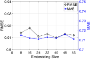
(a) Embedding Size

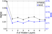
(b) # of Hidden Layers

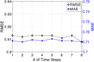
(c) # of Time Steps

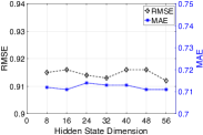
(d) Hidden State Dimension

Figure 2. Parameter sensitivity of NTF($ReLU$) in rating prediction (data from May 2003 to Apr 2004 is used for training and validation, data from May 2004 is used for testing).

(a) Embedding Size

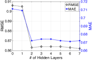
(b) # of Hidden Layers

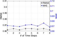
(c) # of Time Steps

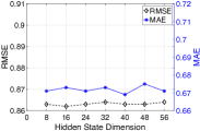
(d) Hidden State Dimension

Figure 3. Parameter sensitivity of NTF($ReLU$) in rating prediction (50% as training data, 10% as validation data and the remaining as testing data).

Table 7. Performance of link prediction on Github archive.

Metrics AUC F1-score Precision Recall AA $0.5159$ $0.1334$ $0.4641$ $0.0768$ PA $0.6443$ $0.3760$ $0.5565$ $0.2842$ PMF $0.7278$ $0.5233$ $0.7507$ $0.4013$ BPMF $0.7165$ $0.5291$ $0.6978$ $0.4250$ NCF $0.7346$ $0.5639$ $0.6421$ $0.5029$ NTF$dot$ $0.7133$ $0.5328$ $0.6681$ $0.4437$ NTF($ReLU$) $0.7841$ $0.6231$ $0.6985$ $0.5612$ NTF($sigmoid$) $0.7787$ $0.6278$ $0.6836$ $0.5803$ NTF($tanh$) $0.7739$ $0.6186$ $0.6765$ $0.5689$

4.2. Rating Prediction and Inference (Q1, Q3 and Q4)

We now compare NTF with state-of-the-art techniques as we introduced above. To investigate the performance of all compared algorithms on different targeted time frames, we show the results from Jan, 2004 to Nov, 2004. The evaluation results are shown in Table 5. Furthermore, we provide analysis on the effects of training ratio (from 30% to 80%) on predictive performance, as shown in Table 6. Based on those evaluation results, we have the following four key observations.

(i) Rating Prediction: Training/test time period. We observe that NTF consistently achieves the best performance over different time frames from Table 5. For example, NTF achieves on average 0.075 and 0.076 (relatively 8.3% and 10.7%) improvements over TDSSM in terms of RMSE and MAE, and 0.075 and 0.075 (relatively 7.4% and 7.8%) improvements over RRN in terms of RMSE and MAE. The evaluation results across different time frames demonstrate the effectiveness of our NTF framework in modeling time-evolving interactions between multiple dimensions in a dynamic scenario. Furthermore, the data becomes more dense as time window slides, i.e., density degree: 2004 Jan-3.67%, 2004 Mar-3.86%, 2004 May-4.11%, 2004 Jul-4.34%, 2004 Sep-4.45% and 2004 Nov-4.57%. We can observe that the performance gain between NTF and other baselines become larger as data becomes sparser, suggesting our NTF is capable of handing sparse relational data.

(ii) Rating Inference: Training/test ratio. Table 6 shows the prediction results when varying the percentage of data in the training set. In this experiment, we fix the percentage of validation data as 10% of the entire dataset. We can observe that obvious improvements can be obtained by our NTF with different sizes of training data, demonstrating that NTF is robust to the data sparsity issue. For example, the average relative improvement over on TDSSM and RRN algorithms are (RMSE: 5.5%, MAE: 7.2%) and (RMSE: 3.1%, MAE: 3.3%), respectively. In addition, we can observe rising trends as the training size increases, which indicate the positive effects of training data size on predicting ratings. Also, the performance gain between NTF and other baselines becomes larger as the training size decreases (more sparse data), which validates the ability of NTF model in predicting interactions with sparse tensor. We can notice that neural network based models (i.e., NCF and RRN) achieve better performance compared with conventional matrix factorization algorithms (i.e., PMF and BPMF) with less training data. This observation suggests that neural network based models are more suitable in sparse relational data. An interesting observation is that BPTF achieves better performance than TDSSM and RRN (neural methods), which indicates the effectiveness to consider the interactions between user, item and time embeddings.

(iii) NTF’s variants. We notice that the performance of our NTF is not sensitive to different activation functions. In addition, our results also indicate that the necessity of our multi-layer perceptron component in NTF for projecting inherent factors into a prediction output by capturing the non-linear relations between them.

(iv) Performance gain analysis. We can observe that NTF shows improvement over both deep collaborative filtering based algorithms (i.e., NCF, PMF, BPMF and BPTF) and recurrent neural networks based schemes (i.e., RRN and TDSSM). In particular, Firstly, this sheds light on the limitations of collaborative filtering based algorithms which ignore the temporal dynamics among the multi-dimensional interactions in the rating data. Secondly, the large performance gap between NTF and recurrent neural network based schemes indicates the limitation of those approaches which only model the sequential pattern of the tensor’s temporal dimension and fail to consider the dependencies between the implicit interactions across dimensions.

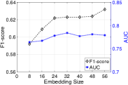
(a) Embedding Size

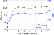
(b) # of Hidden Layers

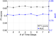
(c) # of Time Steps

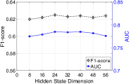
(d) Hidden State Dimension

Figure 4. Parameter sensitivity of NTF($ReLU$) in link prediction on Github dataset.

4.3. Link Prediction (Q2, Q3 and Q4)

Table 7 lists the evaluation results of the link prediction task. In this evaluation, we evaluate all compared models using the the 90% and 10% of Github archive data from first twenty weeks as training and validation data to predict links in the twenty-first week. To construct the testing set, we use the observed links in the twenty-first week as the positive cases and randomly enumerate node pairs and choose unobserved edges as negative cases. We use the same parameter settings as rating prediction task (listed in Table 3). Furthermore, because link prediction problem often suffers from highly unbalanced data (i.e., only 0.02% instances are observed in the GitHub dataset), we sample the negative cases twice as many as positives cases to address this challenge following (Chawla et al., 2004).

Overall, the proposed NTF significantly outperforms other baselines in F1 and AUC. Specifically, the relative improvement of our NTF over NCF is 10.2% and 6.8% in terms of F1-score and AUC respectively. This link prediction task further demonstrate that the NTF framework works well by capturing time-evolving interactions between different dimensions in a non-linear manner.

4.4. Parameter Sensitivity (Q5)

The NTF model involves several parameters (i.e., embedding size in embedding layer, # of hidden layers in MLP, # of time steps and hidden state dimension in LSTM). To investigate the robustness of NTF framework, we examine how the different choices of parameters affect the performance of NTF in both rating and link prediction tasks. Except for the parameter being tested, we set other parameters at the default values (see Table 3).

Rating Prediction. Figure 3 and Figure 2 list the prediction results (measured by RMSE and MAE) as a function of one selected parameter when fixing others. Note that we have two $y$-axes corresponding to RMSE (left-black) and MAE (right-blue) respectively due to their different value ranges. From Figure 3, overall, we can observe that NTF is not strictly sensitive to these parameters, except for # of hidden layers, and can achieve high performance with cost-effective parameters, i.e., the smaller the parameters are, the more efficient the training process will be. Figure 3(b) and Figure 2(b) indicate that model performance becomes stable as long as the number of hidden layers is above 2. From Figure 3(a), we can observe that embedding size is positively correlated with the prediction accuracy and we set it to 32 in our experiment due to the balance between efficacy and computational cost. Additionally, we can observe the low impact of other two parameters (i.e., sequence length and state size in LSTM) on model performance, which suggests the robustness of our NTFin modeling the temporal dynamics of multi-dimensional interactions.

Link Prediction. We also study the parameter sensitivity of NTF as measured by link prediction performance. Figure 4 shows the prediction accuracy (measured by F1-score and AUC) as a function of each of the four parameters when fixing the other three. Figure 4(c) and Figure 4(d) suggest that the sequence length and state size have little impact on prediction accuracy. The increase of link prediction performance converges as the number of hidden layers reaches around 4. Additionally, we can observe that our model shows an increasing trend with an increasing embedding size from Figure 4(a), which is consistent with the observation from the parameter sensitivity evaluation in rating prediction. For NTF without hidden layer (final predictions are directly derived from embedding layer), the performance is suboptimal. This observation verifies our argument that the dot product operation cannot handle the non-linear interactions in tensor factorization and demonstrates the necessity to model the complex interaction dependencies with hidden layers.

5. Related Work

Deep Collaborative Filtering Models. Collaborative Filtering (CF) has been widely applied to various recommendation systems (He et al., 2017; Wu et al., 2016; Li and She, 2017; Hsieh et al., 2017; Chen et al., 2017). In particular, He et al. aimed to develop a neural network collaborative filtering framework by modeling latent features of users and items (He et al., 2017). Wu et al. studied the top-N recommendation problem and proposed a autoencoder based CF method (Wu et al., 2016). Furthermore, a collaborative variational autoencoder has been developed in recommendation systems to consider implicit relationships between items and users (Li and She, 2017). Hsieh et al. studied the connection between metric learning and collaborative filtering. However, these approaches are static models and are lacking when they comes to dynamic scenarios. The proposed NTF addresses this problem by modeling temporal evolution of latent factors in collaborative filtering framework.

Deep Matrix Factorization. With the advent of deep learning techniques, significant effort has been made to develop neural network-based matrix factorization models (Sedhain et al., 2015; Sainath et al., 2013; Kim et al., 2016; Dziugaite and Roy, 2015). Sedhain et al. proposed an autoencoder framework for collaborative filtering (Sedhain et al., 2015). Sainath et al. proposed to apply low-rank factorization to deep neural network models to address the language modeling problem (Sainath et al., 2013). More recently, to address the sparsity problem in recommendation techniques, Kim et al. designed a model which integrates convolutional neural network (CNN) into probabilistic matrix factorization (PMF) (Kim et al., 2016). Dziugaite et al. suggested to replace the the inner product in matrix factorization with the function which is learned from the data together with latent feature vectors. However, the limitation of the above approaches is that they only consider static data instead of dynamic data in which temporal dimension need to be explored. Our work furthers the investigation on this direction by developing the NTF framework to capture the time-evolving temporal dynamics exhibited from relational data with multiple types of entity dependencies, which cannot be handled by previous models.

Applications of Matrix Factorization. There is a good amount of work on the applications of Matrix Factorization. Existing recommendation techniques can be grouped into three categories: content-based algorithms (Cantador et al., 2010; Van den Oord et al., 2013), collaborative filtering based algorithms (Mnih and Salakhutdinov, 2008; Bu et al., 2016) and hybrid algorithms (He and McAuley, 2016; Wang et al., 2015). For example, several content-based recommendation models have been evaluated based on the profiles of users and items (Cantador et al., 2010). Salakhutdinov et al. presented a Probabilistic Matrix Factorization (PMF) model and demonstrated its effectiveness on the movie rating data (Mnih and Salakhutdinov, 2008). Additionally, Wang et al. proposed a hierarchical Bayesian model which integrated content information and collaborative filtering scheme by performing deep representation learning (Wang et al., 2015). Li et al. generalized latent factor framework for social network analysis by modeling homophily. This work can be complementary to the above works in the sense that explicitly exploring temporal dynamics in relational data normally lead to better recommendation results.

6. Conclusion

We developed a novel and general Neural network based Tensor Factorization (NTF) for modeling dynamic relational data that addresses the critical challenge of evolving user-item relational data. By modeling the time-evolving inherent factors and incorporating temporal smoothness constraints on those factors, NTF is capable of capturing both the time-varying interactions across dimensions and the non-linear relations between them. Extensive experiments on two real-world datasets in rating prediction and link prediction tasks show that NTFsignificantly outperforms baseline methods.

Notwithstanding the interesting problem and promising results, some directions exist for future work. We will next incorporate rich heterogeneous auxiliary data to further improve the model. Another possible direction is adapting NTF to a time-sensitive model by analyzing the trade-off between accuracy and complexity.

References

- (1)
- Adamic and Adar (2003) Lada A Adamic and Eytan Adar. 2003. Friends and neighbors on the web. Social networks 25, 3 (2003), 211–230.
- Bengio et al. (2013) Yoshua Bengio, Aaron Courville, and Pascal Vincent. 2013. Representation learning: A review and new perspectives. IEEE transactions on pattern analysis and machine intelligence 35, 8 (2013), 1798–1828.
- Bhargava et al. (2015) Preeti Bhargava, Thomas Phan, Jiayu Zhou, and Juhan Lee. 2015. Who, what, when, and where: Multi-dimensional collaborative recommendations using tensor factorization on sparse user-generated data. In WWW. ACM, 130–140.
- Bu et al. (2016) Jiajun Bu, Xin Shen, Bin Xu, Chun Chen, Xiaofei He, and Deng Cai. 2016. Improving collaborative recommendation via user-item subgroups. TKDE 28, 9 (2016), 2363–2375.
- Cantador et al. (2010) Iván Cantador, Alejandro Bellogín, and David Vallet. 2010. Content-based recommendation in social tagging systems. In Recsys. ACM, 237–240.
- Carroll and Chang (1970) J Douglas Carroll and Jih-Jie Chang. 1970. Analysis of individual differences in multidimensional scaling via an N-way generalization of ”Eckart-Young” decomposition. Psychometrika 35, 3 (1970), 283–319.
- Chawla et al. (2004) Nitesh V Chawla, Nathalie Japkowicz, and Aleksander Kotcz. 2004. Special issue on learning from imbalanced data sets. ACM SIGKDD Explorations (2004), 1–6.
- Chen et al. (2017) Jingyuan Chen, Hanwang Zhang, Xiangnan He, Liqiang Nie, Wei Liu, and Tat-Seng Chua. 2017. Attentive collaborative filtering: Multimedia recommendation with item-and component-level attention. In SIGIR. ACM, 335–344.
- Chung et al. (2014) Junyoung Chung, Caglar Gulcehre, et al. 2014. Empirical evaluation of gated recurrent neural networks on sequence modeling. arXiv preprint arXiv:1412.3555 (2014).
- Chung et al. (2015) Junyoung Chung, Caglar Gulcehre, Kyunghyun Cho, and Yoshua Bengio. 2015. Gated feedback recurrent neural networks. In ICML. 2067–2075.
- Collobert et al. (2011) Ronan Collobert, Jason Weston, Léon Bottou, Michael Karlen, Koray Kavukcuoglu, and Pavel Kuksa. 2011. Natural language processing (almost) from scratch. JMLR 12, Aug (2011), 2493–2537.
- Dziugaite and Roy (2015) Gintare Karolina Dziugaite and Daniel M Roy. 2015. Neural network matrix factorization. ICLR (2015).
- He and McAuley (2016) Ruining He and Julian McAuley. 2016. Ups and downs: Modeling the visual evolution of fashion trends with one-class collaborative filtering. In WWW. ACM, 507–517.
- He and Chua (2017) Xiangnan He and Tat-Seng Chua. 2017. Neural Factorization Machines for Sparse Predictive Analytics. In SIGIR. ACM.
- He et al. (2017) Xiangnan He, Lizi Liao, Hanwang Zhang, Liqiang Nie, Xia Hu, and Tat-Seng Chua. 2017. Neural collaborative filtering. In WWW. ACM, 173–182.
- Hsieh et al. (2017) Cheng-Kang Hsieh, Longqi Yang, Yin Cui, Tsung-Yi Lin, Serge Belongie, and Deborah Estrin. 2017. Collaborative metric learning. In WWW. ACM, 193–201.
- Ioffe and Szegedy (2015) Sergey Ioffe and Christian Szegedy. 2015. Batch normalization: Accelerating deep network training by reducing internal covariate shift. In ICML. 448–456.
- Jozefowicz et al. (2015) Rafal Jozefowicz, Wojciech Zaremba, and Ilya Sutskever. 2015. An empirical exploration of recurrent network architectures. In ICML. 2342–2350.
- Kim et al. (2016) Donghyun Kim, Chanyoung Park, Jinoh Oh, Sungyoung Lee, and Hwanjo Yu. 2016. Convolutional matrix factorization for document context-aware recommendation. In Recsys. ACM, 233–240.
- Kingma and Ba (2014) Diederik Kingma and Jimmy Ba. 2014. Adam: A method for stochastic optimization. arXiv preprint arXiv:1412.6980 (2014).
- Kolda and Bader (2009) Tamara G Kolda and Brett W Bader. 2009. Tensor decompositions and applications. SIAM review 51, 3 (2009), 455–500.
- Koren (2008) Yehuda Koren. 2008. Factorization Meets the Neighborhood: A Multifaceted Collaborative Filtering Model. In KDD ’08. ACM, New York, NY, USA, 426–434.
- Koren et al. (2009) Yehuda Koren, Robert Bell, and Chris Volinsky. 2009. Matrix Factorization Techniques for Recommender Systems. Computer 42, 8 (Aug. 2009), 30–37.
- Li and She (2017) Xiaopeng Li and James She. 2017. Collaborative Variational Autoencoder for Recommender Systems. In KDD. ACM, 305–314.
- Liben-Nowell and Kleinberg (2007) David Liben-Nowell and Jon Kleinberg. 2007. The link-prediction problem for social networks. journal of the Association for Information Science and Technology 58, 7 (2007), 1019–1031.
- Ma et al. (2008) Hao Ma, Haixuan Yang, Michael R. Lyu, and Irwin King. 2008. SoRec: Social Recommendation Using Probabilistic Matrix Factorization. In CIKM. ACM, New York, NY, USA, 931–940.
- Mnih and Salakhutdinov (2008) Andriy Mnih and Ruslan R Salakhutdinov. 2008. Probabilistic matrix factorization. In NIPS. 1257–1264.
- Rigamonti et al. (2011) Roberto Rigamonti, Matthew A Brown, et al. 2011. Are sparse representations really relevant for image classification?. In CVPR. IEEE, 1545–1552.
- Sainath et al. (2013) Tara N Sainath, Brian Kingsbury, Vikas Sindhwani, Ebru Arisoy, and Bhuvana Ramabhadran. 2013. Low-rank matrix factorization for deep neural network training with high-dimensional output targets. In ICASSP. IEEE, 6655–6659.
- Salakhutdinov and Mnih (2008) Ruslan Salakhutdinov and Andriy Mnih. 2008. Bayesian probabilistic matrix factorization using Markov chain Monte Carlo. In ICML. ACM, 880–887.
- Scellato et al. (2011) Salvatore Scellato, Anastasios Noulas, et al. 2011. Exploiting place features in link prediction on location-based social networks. In KDD. ACM, 1046–1054.
- Sedhain et al. (2015) Suvash Sedhain, Aditya Krishna Menon, Scott Sanner, and Lexing Xie. 2015. Autorec: Autoencoders meet collaborative filtering. In WWW. ACM, 111–112.
- Shih et al. (2016) Ting-Yi Shih, Ting-Chang Hou, Jian-De Jiang, Yen-Chieh Lien, Chia-Rui Lin, and Pu-Jen Cheng. 2016. Dynamically Integrating Item Exposure with Rating Prediction in Collaborative Filtering. In SIGIR. ACM, 813–816.
- Shimodaira (2000) Hidetoshi Shimodaira. 2000. Improving predictive inference under covariate shift by weighting the log-likelihood function. Journal of statistical planning and inference 90, 2 (2000), 227–244.
- Song et al. (2016) Yang Song, Ali Mamdouh Elkahky, and Xiaodong He. 2016. Multi-rate deep learning for temporal recommendation. In SIGIR. ACM, 909–912.
- Van den Oord et al. (2013) Aaron Van den Oord, Sander Dieleman, and Benjamin Schrauwen. 2013. Deep content-based music recommendation. In NIPS. 2643–2651.
- Wang et al. (2015) Hao Wang, Naiyan Wang, and Dit-Yan Yeung. 2015. Collaborative deep learning for recommender systems. In KDD. ACM, 1235–1244.
- Wu et al. (2017) Chao-Yuan Wu, Amr Ahmed, Alex Beutel, Alexander J Smola, and How Jing. 2017. Recurrent recommender networks. In WSDM. ACM, 495–503.
- Wu et al. (2016) Yao Wu, Christopher DuBois, Alice X Zheng, et al. 2016. Collaborative denoising auto-encoders for top-n recommender systems. In WSDM. ACM, 153–162.
- Xiong et al. (2010) Liang Xiong, Xi Chen, et al. 2010. Temporal collaborative filtering with bayesian probabilistic tensor factorization. In SDM. SIAM, 211–222.