A General Method for Demand Inversion

Abstract

This paper describes a numerical method to solve for mean product qualities which equates the real market share to the market share predicted by a discrete choice model. The method covers a general class of discrete choice model, including the pure characteristics model in Berry and Pakes (2007) and the random coefficient logit model in Berry et al. (1995) (hereafter BLP). The method transforms the original market share inversion problem to an unconstrained convex minimization problem, so that any convex programming algorithm can be used to solve the inversion. Moreover, such results also imply that the computational complexity of inverting a demand model should be no more than that of a convex programming problem. In simulation examples, I show the method outperforms the contraction mapping algorithm in BLP. I also find the method remains robust in pure characteristics models with near-zero market shares.

1 Introduction

When conducting structural demand estimations, one usually needs to solve the inversion of a demand model given the real market share. The problem often takes the form of a nonlinear equation,

$$\text{find }x\text{ such that }\sigma(x)=\sigma^{*}$$ (1)

where $\sigma^{*}$ is a vector of real market share and $\sigma(x)$ is the model predicted market share given the demand shifter (or mean product quality) $x$. To ensure that the entire estimation procedure is robust and tractable, this inversion problem needs to be solved both precisely and efficiently.

In this paper, I describes a method which transforms the inversion problem (1) into an unconstrained convex optimization problem. This transformation works for a general class of discrete choice models. In particular, it covers the pure characteristics model in Berry and Pakes (2007) and the random coefficient logit model in Berry et al. (1995) (henceforth BLP). As a result of the convex transformation, any convex optimization algorithms can be used to solve the inversion problem. As the algorithms of convex optimization have been extensively studied and their robust implementation are now widely available, the method here is able to solve the inversion problem in (1) efficiently and robustly in both small and large scale problems.

When the demand function $\sigma(\cdot)$ is generated by a mixed logit model, BLP provides an inversion algorithm based on contraction mapping. Their algorithm converges globally at a linear rate, i.e. there exists some $\alpha\in(0,1)$ such that

$$\frac{\left\|x^{(k+1)}-x^{*}\right\|}{\left\|x^{(k)}-x^{*}\right\|}\leq\alpha,$$ (2)

where $x^{*}$ is the solution of (1) and $x^{(k)}$ is the best solution of the algorithm at $k$th iteration. In practice, $\alpha$ could be very close to $1$, which leads to a very slow convergence rate. See our simulation below and Dubé et al. (2012). In contrast, algorithms designed for unconstrained smooth convex optimization can typically converge globally at a superlinear rate, i.e.

$$\lim_{k\to\infty}\frac{\left\|x^{(k+1)}-x^{*}\right\|}{\left\|x^{(k)}-x^{*}\right\|}=0$$

when the Jacobian matrix of $\sigma$ is non-singular. See, for example, Theorem 5.13 in Ruszczyński (2006). As illustrated in simulation experiments, such a difference in convergence speeds could result in considerable efficiency gains in practice.

When the demand function $\sigma(\cdot)$ is generated by pure characteristics model, Berry and Pakes (2007) provides three algorithms to solve the inversion problem, and propose to combine all the algorithms, as none of them works on its own. Song (2006) proposes a detailed procedure on how to combine the Newton-Raphson method into those algorithms. Yet, none of those are fully satisfactory. In particular, none of the existing algorithms ensures global convergence. Also, in practice, when those methods do converges in some cases, their convergence rate tend to be slow. The main challenge here is that the Jacobian matrix of $\sigma$ could be near-singular or singular when the market share of some products is very close or equal to zero. This could happen even if each product has positive share at $\sigma^{*}$, since algorithms can drive $x^{(k)}$ into regions of zero market share during the iteration.

In contrast, the method here still works even if the Jacobian of $\sigma$ is singular. This is due to the fact that some algorithms of convex optimization could still have global convergence (though not necessarily at superlinear rate) even if the Hessian matrix is singular. Among them, the trust region algorithms are very suitable in those singular cases, whose convergence properties and robustness have been extensively studied and developed since 1970’s. For example, see Theorem 5.1.1 in Fletcher (1987) and more general results in Shultz et al. (1985) and Conn et al. (2000).

The rest of the paper is organized as follows. Section 2 presents how to transform the inversion problem into a convex minimization problem. Section 3 conducts simulation experiments on random coefficients logit models and pure characteristics models. All proofs are contained in the Appendix.

2 Convex Transformation

Consider a discrete choice model of $J$ inside products and one outside option. Assume agent $i$’s uility of choosing product $j$ is

$$u_{ji}\coloneqq x_{j}+\epsilon_{ij}$$

where $x_{j}$ is the demand shifter (or mean utility) of product $j$, and $\epsilon_{ij}$ is the taste shock of agent $i$. Normalize agent $i$’s utility from consuming the outside option to be zero. Let $x\coloneqq(x_{1},...,x_{J})$ and $\epsilon_{i}\coloneqq(\epsilon_{i1},...,\epsilon_{iJ})$ be vectors in ^J.

The above framework covers most discrete choice models used in empirical applications. For example, in random coefficients logit models as in BLP, we have $x_{j}=\xi_{j}+z_{j}^{\prime}\beta$ and $\epsilon_{ij}=z_{j}^{\prime}\nu_{i}+\varepsilon_{ij}$ where $\xi_{j}$ is the unobserved product quality, $z_{j}$ is the vector of both exogenous and endogenous product attributes, $\beta$ is the parameter and $\nu_{i}$ is the random coefficient of consumer $i$ and $\varepsilon_{ij}$ is the logistic shock of consumer $i$.

Let $F$ be the distribution of $\epsilon_{i}$. Then, the average welfare of consumer $U(x)$ can be written as

$$U(x)=\mathbb{E}_{F}\max\left(0,\max_{j=1,...,J}(x_{j}+\epsilon_{ij})\right).$$

Let $\sigma(x)\in^{J}$ be the market share of inside goods given $x$ and distribution $F$ and let $\Delta^{J}$ be defined as the simplex

$$\Delta^{J}\coloneqq\Bigg{\{}(s_{1},...,s_{J})\in^{J}:\forall j,\ s_{j}\geq 0\text{ and }\sum_{j}s_{j}\leq 1\Bigg{\}}.$$

Given $F$ and some $\sigma^{*}\in\Delta^{J}$, the inversion problem of the discrete choice model is to find an $x^{*}$ such that $\sigma(x^{*})=\sigma^{*}$ whenever such $x^{*}$ exists. The following theorem transforms such inversion problem into an unconstrained convex optimization problem.

Theorem 1.

Given any $\sigma^{*}\in\Delta^{J}$, $\sigma(x^{*})=\sigma^{*}$ implies

$$x^{*}\in\operatorname*{arg\,min}_{x}\big{(}U(x)-x^{\prime}\sigma^{*}\big{)}.$$ (3)

If distribuion $F$ is non-atomic, the reverse is also true, i.e. condition (3) implies $\sigma(x^{*})=\sigma^{*}$.

Theorem 1 provides a necessary condition for $x^{*}$ to be a solution of the inversion problem. When distribution $F$ is non-atomic, as in most empirical applications, such condition is also sufficient. Since $U(x)$ is a convex function of $x$, solving the inversion problem should be as easy as solving an unconstrained convex optimization problem. Moreover, when $F$ is absolutely continuous, $U(x)$ is twice differentiable so that all smooth convex optimization algorithms can be applied to solve for $x^{*}$ in (3).

To see the intuition behind Theorem 1, let’s assume distribution $F$ is non-atomic. Then, $x^{*}$ is a minimizer of $U(x)-x^{\prime}\sigma^{*}$ if and only if $x^{*}$ satisfies the first order condition,

$$\frac{\partial U(x^{*})}{\partial x}=\sigma^{*}$$ (4)

One can verify that

$$\forall j=1,...,J,\quad\frac{\partial U(x^{*})}{\partial x_{j}}=\mathbb{P}\Bigg{[}x^{*}_{j}+\epsilon_{ij}\geq\max\Big{(}0,\max_{j=1,...,J}(x^{*}_{j}+\epsilon_{ij})\Big{)}\Bigg{]}=\sigma(x^{*})$$ (5)

Combine condition (4) and (5), we know $x^{*}$ minimizes $U(x)-x^{\prime}\sigma^{*}$ if and only if $\sigma(x^{*})=\sigma^{*}$. When $F$ is atomic, condition (4) no longer holds as $U(x)$ could be nondifferentiable, but the same intuition still carries through. See Appendix A for a formal proof of Theorem 1.

In practice, one might consider $\sigma(x)=\sigma^{*}$ as a general nonlinear equation and solve it using Netwon or Quasi-Netwon methods. This approach is known to perform well when the initial value is close enough to the true value, but could fail to converge otherwise. To see how it’s related to the method here, note that if we apply Netwon’s method to solve (3), we get

$$x^{(k+1)}=x^{(k)}-H_{k}^{-1}\Big{(}\frac{\partial U(x^{*})}{\partial x}-\sigma^{*}\Big{)}$$ (6)

where $x^{(k)}$ denotes the solution at iteration $k$ and $H_{k}$ stands for the Hessian matrix of $U(x)$ at $x^{(k)}$. However, in equation (5), we know $\partial U(x)/\partial x=\sigma(x)$ and therefore $H_{k}$ equals the Jacobian matrix of $\sigma(x)$ at $x^{(k)}$. As a result, iteration (6) is equivalent to

$$x^{(k+1)}=x^{(k)}-H_{k}^{-1}\cdot(\sigma(x^{(k)})-\sigma^{*})$$

which actually is the iteration step when we apply Newton-Raphson’s method to solve equation $\sigma(x)=\sigma^{*}$. However, there is a key difference between solving the convex optimization problem in (3) and solving the nonlinear equation $\sigma(x)=\sigma^{*}$: Theorem 1 enable us to utilize the objective function $U(x)-x^{\prime}\sigma^{*}$. Such extra information is not used in solving nonlinear equation $\sigma(x)=\sigma^{*}$, but is utilized in solving its transformed problem (3). Indeed, this extra information plays an essential role in ensuring the global convergence of convex optimization algorithms, especially when $H_{k}$ is singular or nearly singular. As an example of such global convergence results, see Theorem 5.1.1 in Fletcher (1987). In the following simulation experiments, we can see clearly how this difference results in different degrees of robustness.

3 Simulation Experiments

In this section, I conduct simulation experiments on random coefficients logit models and pure characteristics models. In each experiment, I solve the inversion problem by minimizing the convex function in Theorem 1, and compare its robustness and speed with other methods.

3.1 Random Coefficients Logit Models

I construct the following random coefficients logit model. Let $J$ denote the number of products and $M$ denote the dimension of product attributes. In each simulation, we draw parameter $\beta$ from uniform distribution in $[0,1]^{M}$, and draw product attributes $z_{1},...,z_{J}$ independently from a normal distribution $N(0,I_{M})$ where $I_{M}$ is the $M$ dimensional identity matrix. We then draw $n=5000$ i.i.d. random coefficients $\nu_{i}$ from $N(0,I_{M})$. Given $\beta$, $\{z_{j}\}$ and $\{\nu_{i}\}$ in each simulation, consumer welfare $U(x)$ and market share $\sigma(x)$ can be calculated as

$$U(x) = \frac{1}{n}\sum_{i=1}^{n}\log\Big{(}1+\sum_{q=1}^{J}\exp(x_{q}+z^{\prime}_{q}\nu_{i})\Big{)}+\gamma$$

$$\sigma_{j}(x) = \frac{1}{n}\sum_{i=1}^{n}\frac{\exp(x+z_{j}^{\prime}\nu_{i})}{1+\sum_{q=1}^{J}\exp(x_{q}+z^{\prime}_{q}\nu_{i})}\quad j=1,...,J$$

where $\gamma$ is Euler’s constant. Let

$$x^{*} = (z_{1}^{\prime}\beta,...,z_{J}^{\prime}\beta)$$

$$\sigma^{*} = \sigma(x^{*})$$

In the simulation experiments, I solve the inversion problem $\sigma(x)=\sigma^{*}$ using the following two methods:

1. Contraction Mapping in Berry et al. (1995).

2. Trust-region algorithm applied to convex optimization (1).

As both methods ensures global convergence, our focus here is to compare their convergence rate.

I conduct $100$ simulation experiments with $J=10$ and $M=5$. Within each simulation experiment, a new set of $\beta$, $\{z_{j}\}$ and $\{\nu_{j}\}$ is drawn and each algorithm takes $x_{1}=x^{*}+\delta$ as its initial point, where $\delta$ is a random vector drawn in each experiment with $\left\|\delta\right\|=20$. In each iteration $k$, I record the maximum norm of the error, $\left\|\sigma(x^{(k)})-\sigma^{*}\right\|_{\infty}\coloneqq\max_{j}(|\sigma_{j}(x^{(k)})-\sigma^{*}_{j}|)$, where $x^{(k)}$ is the best solution up to iteration $k$. Algorithm (i) calculates $\sigma(x)$ once every iteration, and Algorithm (ii) calculates $U(x)$, $\sigma(x)$ and the Hessian matrix of $U(x)$ once every iteration.

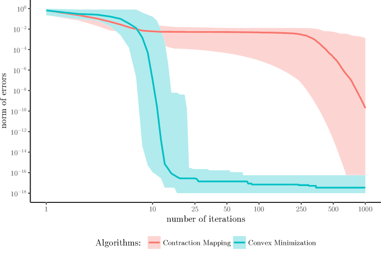
Figure 1: Inversion of Random Coefficients Logit Demand

The result is shown in Figure 1, where I plot the area between the worst and the best norm of the error among all simulation experiments, and plot the median of the norm of these errors in solid lines. The method based on convex optimization clearly outperforms the contraction mapping algorithm. After only $25$ iterations of the convex optimization method, the norm of error is less than $10^{-15}$ in all simulation experiments. In contrast, after $250$ iterations of the contraction mapping algorithm, the norm of error is still larger than $10^{-3}$ in more than half of the simulation experiments. Note the error curve of the contraction mapping algorithm is almost flat during iteration $10$ to $250$, indicating the Lipschitz constant of the algorithm, i.e. the $\alpha$ in (2), could be very close to $1$. This is the major reason why the contraction mapping algorithm can be very slow. More discussion on this can be founded in Dubé et al. (2012).

3.2 Pure Characteristics Models

Let’s construct a pure characteristics model as follows. Let $J$ denote the number of products and $M$ denote the dimension of product attributes. For any vector $y$ in ^M, let $y^{(1)}$ denote its first coordinate and $y^{(-1)}$ denotes its remaining $M-1$ coordinates.

In each simulation experiment, we normalize $\beta^{(1)}=1$ and draw $\beta^{(-1)}$ from a uniform distribution on $[0,1]^{M-1}$. We then draw $z_{1},...,z_{J}$ independently from a normal distribution $N(0,I_{M})$. As for random coeffcients $\nu$, we simulate $n=5000$ i.i.d $\nu^{(-1)}_{i}$ samples from $N(0,I_{M-1})$. Given $\beta$, $\{z_{j}\}$ and $\{\nu^{(-1)}_{i}\}$ in each simulation, consumer welfare $U(x)$ and market share $\sigma(x)$ can be calculated as

$$U(x) = \frac{1}{n}\sum_{i=1}^{n}\int u(x_{i},z_{i},\nu_{i}^{-1},\nu^{(1)})\mathrm{d}\varphi(\nu^{(1)})$$

$$\sigma_{j}(x) = \frac{1}{n}\sum_{i=1}^{n}\int\mathbbm{1}\left(x_{j}+z_{j}^{(-1)\prime}\nu_{i}^{(-1)}+z_{j}^{(1)}\nu^{(1)}\geq u(x_{i},z_{i},\nu_{i}^{-1},\nu^{(1)})\right)\mathrm{d}\varphi(\nu^{(1)})$$

where $\varphi(\cdot)$ denotes the density function of the standard normal distribution $N(0,1)$, and

$$u(x_{i},z_{i},\nu_{i}^{(-1)},\nu_{i}^{(1)})\coloneqq\max\left\{0,\max_{j}\left(x_{j}+z_{j}^{(-1)\prime}\nu_{i}^{(-1)}+z_{j}^{(1)}\nu^{(1)}\right)\right\}$$

The, the market share $\sigma^{*}$ and its true inversion $x^{*}$ can be written as

$$x^{*} = (z_{1}^{\prime}\beta,...,z_{J}^{\prime}\beta)$$

$$\sigma^{*} = \sigma(x^{*})$$

In the simulations, I solve the inversion problem $\sigma(x)=\sigma^{*}$ using the following two methods:

1. Trust-region algorithm applied directly to nonlinear equation $\sigma(x)=\sigma^{*}$.

2. Trust-region algorithm applied to convex optimization (1).

To implement Algorithm (a), I utilize Matlab function fsolve with its algorithm option set to trust-region. When implementing Algorithm (b), I use a self-implemented trust-region procedure. Algorithm (b) is guaranteed to converge no matter what the initial value is, while Algorithm (a) only ensures local converge when the initial value is close enough to the true solution. Therefore, we mainly focus on comparing the robustness of different methods.

Similar to the previous simulation experiments, I conduct $100$ simulations experiments with $J=10$ and $M=5$. Within each simulation experiment, a new set of $\beta^{(-1)}$, $\{z_{j}\}$ and $\{\nu_{j}^{(-1)}\}$ is drawn and each algorithm takes $x_{1}=x^{*}+\delta$ as its initial point, where $\delta$ is a random vector drawn in each experiment with $\left\|\delta\right\|=20$. In each iteration $k$, I record the maximum norm of the error, $\left\|\sigma(x^{(k)})-\sigma^{*}\right\|_{\infty}\coloneqq\max_{j}(|\sigma_{j}(x^{(k)})-\sigma^{*}_{j}|)$, where $x^{(k)}$ is the best solution up to iteration $k$. Algorithm (a) calculates $\sigma(x)$ and the Hessian matrix of $U(x)$ once every iteration, and Algorithm (b) calculates $U(x)$, $\sigma(x)$ and the Hessian matrix of $U(x)$ once every iteration.

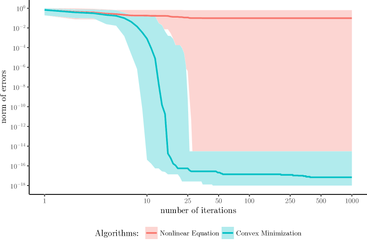
Figure 2: Inversion of Pure Characteristics Demand

The result is shown in Figure 2, where I plot the area between the worst and the best norm of erros of all simulation experiments. I also plot the median in solid lines. Clearly, the method based on convex minimization dominates, in terms of both efficiency and robustness. After $25$ iterations of the convex minimization method, the norm of errors is less than $10^{-14}$ in all simulation experiments. In contrast, the method directly solving the nonlinear equation $\sigma(x)=\sigma^{*}$ is much less robust. It fails to converge in more than half of the experiments. And, when the norm of errors does converges, it converges slower than the convex minimization method.

The performance difference between these two methods is mainly driven by the singularity of the Hessian matrix. In more than half of our simulation experiments, the minimum market share of products, $\min(\min_{j}\sigma^{*}_{j},1-\sum_{j}\sigma^{*}_{j})$, is smaller than $10^{-14}$. In some of the experiments, the minimum market share of products is even zero. In these cases, the Hessian matrix of $U(x)$, or equivalently the Jacobian matrix of $\sigma(x)$, is near singular or singular. As discussed in the end of Section 2, the method based on the convex optimization is able to utilize more information than the method solving the nonlinear equation directly, which ensures its strong convergence property even in those singular cases.

Appendix A Proof of Theorem 1

First of all, by Theorem 23.5 in Rockafellar (1997), in particular, by the equivalence of condition (a) and (b) in Theorem 23.5, we know condition (3) is equivalent to $\sigma^{*}\in\partial U(x^{*})$, where $\partial U(x)$ stands for the subgradient of $U(x)$ with respect to $x$.

Let $y_{i}(x)\in^{J}$ be the choice of agent $i$, with $y_{i,j}=1$ if product $j$ is chosen and $y_{i,j}=0$ if not chosen. Then,

$$y_{i}(x)\in\partial\tilde{U}(x,\epsilon_{i})$$

where $\tilde{U}(x,\epsilon_{i})=\max\left(0,\max_{j=1,...,J}(x_{j}+\epsilon_{ij})\right)$ is individual $i$’s utility with her random $\epsilon_{i}$, and $\partial\tilde{U}(x,\epsilon_{i})$ stands for the subgradient of $\tilde{U}(x,\epsilon_{i})$ with respect to $x$. With these notations, we can write average consumer welfare as $U(x)=\mathbb{E}_{F}\tilde{U}(x,\epsilon_{i})$ and market share as $\sigma(x)=\mathbb{E}_{F}y_{i}(x)$.

By Proposition 2.2 in Bertsekas (1973), we know

$$\mathbb{E}_{F}y_{i}(x)\in\partial\mathbb{E}_{F}\tilde{U}(x,\epsilon_{i}),$$

or, equivalently, $\sigma(x)\in\partial U(x)$. Therefore, if $\sigma(x^{*})=\sigma^{*}$, we must have $\sigma^{*}\in\partial U(x^{*})$. Hence, we know condition (3) must hold.

If distribution $F$ is non-atomic, then $\partial\tilde{U}(x,\epsilon_{i})=\{y_{i}\}$ almost surely. By proposition 2.2 in Bertsekas (1973), this implies $\partial\mathbb{E}_{F}\tilde{U}(x,\epsilon_{i})=\{\mathbb{E}_{F}y_{i}\}$, or equivalently, $\partial U(x)=\{\sigma(x)\}$. When condition (3) holds, we know $\sigma^{*}\in\partial U(x^{*})$ and hence, $\sigma^{*}=\sigma(x^{*})$.

References

- (1)
- Berry and Pakes (2007) Berry, Steven and A. Pakes, “The Pure Characteristics Demand Model,” International Economic Review, 2007, 48 (4), 1193–1225.
- Berry et al. (1995) , J. Levinsohn, and A. Pakes, “Automobile Prices in Market Equilibrium,” Econometrica, July 1995, 63 (4), 841.
- Bertsekas (1973) Bertsekas, D. P., “Stochastic optimization problems with nondifferentiable cost functionals,” Journal of Optimization Theory and Applications, August 1973, 12 (2), 218–231.
- Conn et al. (2000) Conn, A. R., N. I. M. Gould, and P. L. Toint, Trust-region methods MPS-SIAM series on optimization, Philadelphia, PA: Society for Industrial and Applied Mathematics, 2000.
- Dubé et al. (2012) Dubé, Jean-Pierre, J. T. Fox, and C.-L. Su, “Improving the Numerical Performance of Static and Dynamic Aggregate Discrete Choice Random Coefficients Demand Estimation,” Econometrica, 2012, 80 (5), 2231–2267.
- Fletcher (1987) Fletcher, R., Practical methods of optimization, 2nd ed ed., Chichester ; New York: Wiley, 1987.
- Rockafellar (1997) Rockafellar, R. Tyrrell, Convex analysis Princeton landmarks in mathematics and physics, Princeton, NJ: Princeton Univ. Press, 1997.
- Ruszczyński (2006) Ruszczyński, Andrzej P., Nonlinear optimization, Princeton, N.J: Princeton University Press, 2006.
- Shultz et al. (1985) Shultz, Gerald A., R. B. Schnabel, and R. H. Byrd, “A Family of Trust-Region-Based Algorithms for Unconstrained Minimization with Strong Global Convergence Properties,” SIAM Journal on Numerical Analysis, 1985, 22 (1), 47–67.
- Song (2006) Song, Minjae, “Estimating the Pure Characteristics Demand Model: A Computational Note,” Working Paper, 2006.