Enabling Interactive Mobile Simulations Through Distributed Reduced Models

Abstract

Currently, various hardware and software companies are developing augmented reality devices, most prominently Microsoft with its Hololens. Besides gaming, such devices can be used for serious pervasive applications, like interactive mobile simulations to support engineers in the field. Interactive simulations have high demands on resources, which the mobile device alone is unable to satisfy. Therefore, we propose a framework to support mobile simulations by distributing the computation between the mobile device and a remote server based on the reduced basis method. Evaluations show that we can speed-up the numerical computation by over 131 times while using 73 times less energy.

1 Introduction

Currently, several hardware and software companies announced or already released augmented reality devices, such as Microsoft’s Hololens, Sony’s SmartEyeglass, or Epson’s Moverio Pro. Using such devices allows the user to see the real world augmented with additional information, such as the state of the object the user is looking at or even holograms displaying 3D scenes over the real world.

One interesting application of such devices is to display the result of numerical simulations. Having simulation results ubiquitously available supports engineers or decision makers in the field [1, 2, 3]. As an example for such pervasive applications, consider an engineer who has to find a solution for placing a hot exhaust tube during deployment of a machine in a factory. To this end, the engineer uses her augmented reality device, which directly shows the heat of the surface of the tube as if the machine were operational. She can adjust the airflow surrounding the tube by changing parameters. The application enables her to see the heat even in complex regions, e.g., in bends, and she can place the tube according to surrounding materials. Other applications for mobile simulations are the visualization of simulation results based on readings from nearby sensors for Internet of Things applications or simulations on drones in order to exploit the wind-field for energy-efficient flight routes [4].

The main challenge for the computation of simulation results on mobile devices is the computational complexity. While it is feasible to visualize even complex 3D data using dedicated GPUs on the mobile device, calculating this data is still challenging due to slow processors and limited energy resources of mobile devices. Therefore, we present an approach to support interactive simulations on resource-constrained mobile devices by distributing computations between the mobile device and a server infrastructure. Moreover, the programmer should be able to re-use existing simulation code. Such code is typically optimized for the server architecture, which might include special hardware, such as additional GPUs, or vector processing instruction sets, not available on the mobile device. Besides the computational aspect, the communication overhead is critical for an efficient distributed execution on mobile devices and a remote server. Therefore, we also need to minimize the amount of data communicated between mobile device and server.

To support numerical simulations on mobile devices, we present a middleware in this paper that allows for the efficient distribution of simulations between a mobile device and remote server infrastructure. This middleware is based on the so-called Reduced Basis Method (RBM) that allows for reducing the complexity of simulations by pre-calculating an optimized basis reducing the dimensionality of the simulation problem. The basic idea of applying the RBM to distributed mobile simulations is to calculate the reduced basis remotely on a server and to transfer the basis to the mobile device. Using the reduced basis, the mobile device is able to perform simulations locally with reduced computational overhead to calculate approximate solutions, where the reduction of quality of approximate solutions is well-defined and bounded.

Using the RBM for efficient distributed simulations is not completely novel and has already been proposed in [5]. However, approaches so far are rather static. They calculate and deploy a basis once, which is then used for all subsequent simulations. In contrast, our approach allows for the dynamic adaptation of the basis during runtime.

In detail, the contributions of this article are:  (1) identification of a new class of serious augmented reality applications, namely interactive mobile simulations; (2) presentation of a mobile simulation middleware that supports the programmer in implementing such applications; (3) two approaches to enable mobile interactive simulations with and without a-priori known parameter restrictions; (4) two approaches optimizing the bottleneck on mobile devices, which is reading data from internal storage; (5) one approach to improve the pre-calculation step of the RBM for our mobile approach; (6) real-world evaluations, including comparison of run-time and energy consumption of the methods, showing that our approaches are up to over 131 times faster and consume 73 times less energy compared to offloading everything to a server.

This work is an extension of our prior work [6], in which we presented two approaches to enable mobile interactive simulations and one approach to reduce the amount of data to be read from internal storage. In this work, we extend our previous work by another approach for reducing the read operations which is built on top of the previously introduced approach. Additionally, we present a novel approach for the optimized pre-calculation on the server that further reduces the energy cost during runtime on the mobile device.

The rest of the paper is structured as follows. Section 2 provides background on the RBM followed by the system model in Section 3. Section 4 introduces a basic approach, which will be modified to the adaptive approach in Section 5. In order to reduce the number of snapshots during the computation, we present the subspace approach and the reorder approach in Section 6 and Section 7. Section 8 introduces a new approach for pre-processing on the server in order to improve the reorder approach. Section 9 evaluates our approaches, before we discuss related work in Section 10 and conclude the paper.

2 The Reduced Basis Method

Our approach to enable interactive mobile simulations utilizes the Reduced Basis Method (RBM) to solve complex numerical problems by calculating parts of the simulation on a remote server infrastructure. In order to better understand the problem to be solved and the solution, we first give a brief introduction to the numerical problems to be solved and the RBM in this section, before we explain the approach in the following section. A more in depth explanation of RBM can be found in [7, 8, 9].

2.1 The Full Numerical Problem

Simulations predict the behavior of a system based on a model. Commonly, such models are described using differential equations. Such equations need to be discretized, which leads to large algebraic equations of the form $A\cdot u=f$, where $A$ is a given matrix, $f$ is a given vector called the right-hand side, and $u$ is the unknown solution. We call this equation the full problem.

Simulation models contain parameters describing different properties of the system that can be changed. Such parameters can be used to interact with the system, e.g., to insert sensor readings or user input. To express the dependency on parameters, we formulate the full problem as

$$\mathbf{A}(\mu)\cdot\mathbf{u}(\mu)=\mathbf{f}(\mu)$$ (1)

where $\mu$ is a vector including all parameters of the simulation.

2.2 Parameter Separable Matrices

The essential part of RBM is the parameter separability of the matrix $A(\mu)$ and the right-hand side $f(\mu)$. Parameter separability of a vector or matrix $M$ is given if we know scalar functions $\theta_{i}$ that map from the parameter space to real numbers and matrices $M_{i}$ that have the same shape as $M$ such that

$$\mathbf{M}(\mu)=\sum_{i}\theta_{i}(\mu)\mathbf{M}_{i}.$$ (2)

Such a representation can be derived from the model equation or using Empirical Interpolation Methods [10].

2.3 The Reduced Problem

The RBM represents approximate solutions of the full numerical problem as linear combination of snapshots. Snapshots are pre-computed and linear independent solutions for typical parameters. The snapshots form the snapshot matrix $V$. Therefore, the approximation to the real solution $u(\mu)$ is $Vu_{V}(\mu)\approx u(\mu)$, where vector $u_{V}(\mu)$ is called the reduced solution. The size of the reduced solution is the number of snapshots.

Using $Vu_{V}(\mu)\approx u(\mu)$, we can rewrite Equation 1 as $A(\mu)Vu_{V}(\mu)\approx f(\mu)$. This is an overdetermined system. Therefore, we multiply the full problem from left with $V^{T}$, which yields our reduced problem $V^{T}A(\mu)Vu_{V}(\mu)=V^{T}f(\mu)$. We call $A_{V}(\mu):=V^{T}A(\mu)V$ the reduced matrix with snapshot matrix $V$. Notice that $A_{V}(\mu)$ is again a separable matrix. The matrices ($V^{T}A_{i}V$) in this separation can be pre-computed, and the matrix $A_{V}(\mu)$ can be rapidly assembled:

$$\mathbf{V}^{T}\mathbf{A}(\mu)\mathbf{V} =\mathbf{V}^{T}\left(\theta_{1}\left(\mu\right)\mathbf{A}_{1}+\cdots+\theta_{m}(\mu)\mathbf{A}_{m}\right)\mathbf{V}$$

$$=\theta_{1}(\mu)\mathbf{V}^{T}\mathbf{A}_{1}\mathbf{V}+\cdots+\theta_{m}(\mu)\mathbf{V}^{T}\mathbf{A}_{m}\mathbf{V}$$

Similarly, $f_{V}(\mu):=V^{T}f(\mu)$ can be partially pre-computed and rapidly assembled.

The process of computing a reduced solution is now to solve $A_{V}(\mu)u_{V}(\mu)=f_{V}(\mu)$ and then to reconstruct $u_{V}(\mu)$ to the full problem space by multiplication with $V$. Solving the low dimensional problem is much faster than solving the full problem, as the low dimensional problem has only the size of the number of snapshots, which is typically much smaller than the full problem size.

Using a reduced basis instead of solving the full problem typically degrades the quality of the solution. To express the quality of the solution, we use the residual norm of the approximation as error indicator. The residual is the difference of $A(\mu)Vu_{V}(\mu)$ and the right-hand side $f(\mu)$. If the residual $r$ is $0$, the approximation $Vu_{V}(\mu)$ is the exact solution $u(\mu)$ of the algebraic problem $A(\mu)u(\mu)=f(\mu)$. The residual is a well-known measurement for approximations in numerics and can be computed very efficiently using pre-computation (c.f. Appendix). This allows for fast quality checks for specific parameters during run-time.

2.4 The Basis Generation Process

Using the residual as error indicator, the snapshots can be computed from a training set of parameters using a greedy approach [11].

1:function GreedyBasisGeneration($\mathit{train\_set},max\_res$)

2:    $\mathit{basis}\leftarrow$ initial basis

3:    $\mathit{residuals}[\mu]\leftarrow\mathit{basis}.\mathit{residual}(\mu)\quad\forall\mu\in\mathit{train\_set}$

4:    while $\mathsf{max}(\mathit{residuals})\geq\mathit{max\_res}$ do

5:         $\mu^{*}\leftarrow\mathsf{max}(\mathit{residuals}).\mathit{key}$

6:         $\mathit{solution}\leftarrow$ solution of the full problem for $\mu^{*}$

7:         add $\mathit{solution}$ to $\mathit{basis}$

8:         $\mathit{residuals}[\mu]\leftarrow\mathit{basis}.\mathit{residual}(\mu)\quad\forall\mu\in\mathit{train\_set}$     

9:    return $\mathit{basis}$

Figure 1: Greedy approach for generation of a reduced basis, where $\mathit{train\_set}$ is a set of parameters and $\mathit{max\_res}$ is the maximum residual threshold.

Figure 1 depicts the pseudo code of the greedy basis generation method. The user provides a set of training parameters ($\mathit{train\_set}$) and a maximum threshold for the residual ($\mathit{max\_res}$). The initial basis can be either an existing basis, or the reduced basis based on the evaluation of a random training parameter. The algorithm will terminate when the generated basis provides a residual norm lower than the provided threshold for all parameters in the training set. In every iteration of the loop, one solution of the full problem is computed and added to the basis. For this computation, the parameter that yields the maximum residual norm using the current basis is chosen.

2.5 Limitations of the Reduced Basis Method

The RBM converts the full dimensional problem into a lower dimensional problem by computation on snapshots. The dimension of the reduced problem depends on the number of snapshots. The number of snapshots depends on the characteristics of the problem and the quality required by the user. The here introduced method works only for stationary problems without any changes to the geometry. However, in recent literature, RBM approaches for time-dependent problems or problems with changing geometry have already been proposed [9, 12]. While such approaches could be used in the approaches presented in this article, we will focus on stationary problems and fixed-geometry.

3 System Model

Next, we describe the assumptions on hardware and software components, as well as the interfaces between the components in our mobile simulation middleware. Figure 2 depicts an overview of the system components and interfaces.

Figure 2: System Model

3.1 System Components

The system consists of two compute nodes, namely the mobile device and the server. Both nodes are connected via a wireless communication channel. Furthermore, the system consists of two software components provided by the application programmers, the numerical simulation and the user application, and the middleware, which defines the distribution of computations.

The mobile device is the augmented reality headset carried by the user. Energy consumption on the mobile device is critical as it is battery-powered. There are two distinct energy consumers on the mobile device, the processor and the communication module.

In contrast to mobile devices, the server provides fast execution. It can be scaled-up by using specialized hardware, such as GPUs for efficient computation of numerical codes, or scaled-out by adding more servers in a cloud infrastructure.

For the wireless communication channel between mobile device and server, we assume data rates of multiple Mbit/s, as provided by state of the art wireless communication technologies like IEEE 802.11 (WiFi) or 4G cellular networks.

The numerical simulation is implemented by the simulation expert. The simulation problem is implemented as a separable matrix $A(\mu)$ and a separable vector $f(\mu)$ representing the simulation problem $A(\mu)\cdot u(\mu)=f(\mu)$ as described in Section 2. Parameters of the simulation model are represented by a vector $\mu$. Additionally, the simulation expert has to define the quality requirements of the application. The quality has to be specified by two parameters. The first parameter, say $\mathcal{D}$, is the discretization of the full problem. The second, say $r_{\textit{max}}$, is the maximum residual value, which is an indicator for the error introduced by the RBM.

The user application is implemented by the application programmer. It sends queries to the middleware. Queries contain a parameter vector $\mu$, which encodes sensor data or user input. When the query is answered, the user application visualizes the simulation results on the augmented reality headset.

The mobile simulation middleware connects the components. It executes code on the server and on the mobile device. Intuitively, the reduced basis method will be used to answer queries with low latency on the mobile device, and the compute-intensive pre-computation of the reduced basis will be performed on the server.

3.2 Interfaces

The numerical simulation and the user application provide interfaces for the mobile simulation middleware. Figure 3 shows an overview of all interfaces. There are three methods of the numerical simulation to be called by the middleware and one method called by the user application.

Figure 3: Interfaces for the mobile simulation middleware.

The numerical simulation has to implement three interfaces providing the problem matrix, the right-hand side, and solutions to the simulation problem. The problem matrix and the right-hand side has to be provided in parameter separable form. This call is only depending on the quality parameter $\mathcal{D}$. The interface to provide solutions of the simulation problem, called snapshot, provides $u(\mu)$ as the solution of the problem $A(\mu)u(\mu)=f(\mu)$ depending on the parameter. Notice that the implementation of the interface to provide snapshots is optional. The mobile simulation middleware could also use a generic algorithm to solve this problem. However, the simulation expert usually knows which solver should be used to solve the simulation problem efficiently.

The user application sends queries to the mobile simulation middleware. Queries contain the parameter $\mu$. The middleware will return an approximate solution which fulfills the quality requirements given by the simulation expert.

4 Basic Approach

In the following, we present our approaches for the efficient execution of mobile simulations using the Reduced Basis Method. We first present a basic approach in this section, which is then further extended to improve adaptability and energy efficiency in the following sections.

The basic approach for processing queries with different parameters on the mobile device consists of four steps: (1) generation of the reduced basis on the server; (2) communication of the reduced basis from the server to the mobile device where the reduced basis is stored on the internal storage; (3) loading the reduced basis from the internal storage of the mobile device; (4) processing queries on the mobile device using the reduced basis.

The generation of the basis is executed on the server. To this end, the mobile device sends a request to the server which contains all information needed for the basis generation process. This includes the training set and the minimum quality as maximum residual threshold, which depends on the application. The training set can be given by the domain expert or, in applications where sensor values are read, the mobile device can first collect some sensor data, statistically obtain the distribution of the parameter $\mu$, and then use this distribution to create the training set for the reduced basis.

Once the basis has been generated on the server, it is sent to the mobile device. The mobile device stores the basis on internal storage. Notice that the pre-computation of the reduced basis can take multiple minutes, depending on the numerical simulation code, the training set, and the number of snapshots needed to achieve the quality as specified. However, this step is only needed once for initialization and should not be performed when latency-sensitive queries need to be processed.

Data	Size
Snapshots	$n\cdot d$
Reduced Problem Matrix	$S_{A}\cdot n^{2}$
Reduced Right Hand Side	$S_{f}\cdot n$
Residual Computation Matrices	$S_{A}^{2}n^{2}+2S_{A}S_{f}n+S_{f}^{2}$

Figure 4: Size of the reduced basis in floating point numbers.

Figure 4 lists the size of the data communicated and stored on the mobile device. The size of the data depends on the number of snapshots $n$, the number of discretization points of the full problem $d$, and the number of summands in the separation of the problem matrix $S_{A}$ and the right-hand side $S_{f}$. The number of discretization points $d$, which depends on $\mathcal{D}$, is by far the largest part, typically multiple thousand floating point numbers (in our evaluation up to $65536$ with $\mathcal{D}=256$). The number of snapshots depends on the residual and is typically below $30$ in our experiments. Numbers $S_{A}$ and $S_{f}$ are constant for a given problem. In our evaluation these values were $4$ and $1$.

After the basis is stored in a file on the mobile device, this file needs to be read by the middleware on the mobile device. As the file size for the reduced basis can grow rapidly, reading the data from the file can take up to seconds. However, this step is needed only once and can be performed when the user starts the user application, long before the first query will be received by the middleware. The basis can then be stored in memory for processing of multiple queries.

Processing a query is then straightforward as described in Section 2.3. First, we need to assemble the reduced system and then compute the solution of the reduced problem. After that, we need to multiply the solution with the snapshots to get an approximate solution of the full problem. In addition to the approximate solution, we also calculate the residual of this approximation and provide this information to the application. Notice that fulfilling the quality constraints for queries with parameters outside the range of the training set cannot be guaranteed using this approach. However, it is known that the quality of the result does depend on the region of the parameters rather than the density or specific choice of parameters in the training set [9]. Therefore, for queries with parameters inside the range of the training set, the resulting approximation should have high quality. Furthermore, for many practical problems, the parameter region is known a priori by physical constraints. For example, if one parameter is the heat conductivity of some material, the application can request the reduced basis in the range of all materials to be used for the specific purpose, e.g., all exhaust tubes ever used by the company.

The basic approach has several drawbacks. First, the parameter range needs to be known before the basis generation process. If the parameter range changes, e.g., because the range of sensor values changes, the approach has to start from scratch. We therefore present an adaptive approach in the next section. Another problem is the latency and energy overhead introduced by reading the reduced file from internal storage of the mobile device. This is significantly improved using the subspace approach, which will be presented in Section 6.

5 Adaptive Approach

If the parameter range and distribution are not known a priori, the basic approach might not be able to fulfill the constraint on quality for all queries. We therefore introduce an adaptive approach next that refines the basis during runtime. This approach is more flexible and also suitable for harder simulation problems, i.e., problems that need more snapshots to fulfill the user requirements.

5.1 Overview

The adaptive approach builds upon the basic approach. Similar to the basic approach, some initial reduced basis is made available on the mobile device as described in the previous section. However, in contrast to the basic approach, when a new query $q$ arrives, the adaptive approach first computes the residual of the approximate solution provided by the RBM. If the residual fulfills the quality requirements of the application, the query will be answered with the approximate solution. If the residual does not fulfill the requirements of the application, the mobile device will request an update of the reduced basis from the server. Once the mobile device receives the update, it can again compute the approximate solution, which will—as a property of the RBM—return the exact solution of the full problem. Figure 5 depicts the pseudocode of the adaptive approach.

1:function onQueryReceived($q$)

2:    $\mu\leftarrow$ parameter of request $q$

3:    $\mathit{basis}\leftarrow$ basis available on mobile

4:    if $\mathit{basis}.\mathit{residual}(\mu)\leq max\_res$ then

5:         return approximate solution using $\mathit{basis}$     

6:    send $\mu$ to server; receive basis update

7:    apply basis update to $\mathit{basis}$

8:    return approximate solution using $\mathit{basis}$

Figure 5: Pseudocode for the adaptive approach.

In the following, we will describe the parts of the approach, including the computation of the error indicator and content of the server request, and the processing of the update on the server.

5.2 Error Indicator and Server Requests

In addition to the basic approach, for handling query $q$, the mobile device has to compute error indicators for the approximate solution provided by the RBM. This error indicator represents the quality of the approximate solution. One very generic error indicator is the residual. The computation of the residual can be implemented very efficiently by exploiting the parameter separability (c.f. Appendix).

Once the mobile device has computed the error indicator, it can check if the quality bounds of the user can be met. If the result is insufficient, the mobile device will request a basis update from the server. This basis update contains the parameter $\mu$ of the query and the identifier of the reduced basis which is currently used. As an identifier, the parameters of the snapshots and the discretization of the underlying numerical simulation can be used.

5.3 Computation on the Server

When an update request with parameter $\mu$ and an identifier of the reduced basis is received by the server, the server first loads the properties of the reduced basis. It then computes a solution of the full problem with parameter $\mu$ and the discretization settings of the reduced basis. After computation of the full solution, this solution is orthogonalized to other basis vectors and is normalized to obtain more robust numerical systems. The server then computes the updated separable problem matrix and the separable right-hand side (c.f. Section 4). Last, the updated residual matrices are computed. All of these operations require high-dimensional and costly operations. However, the most time consuming operation is the computation of the full solution on the server. Therefore, there is only little overhead compared to a pure offloading approach, where only the full problem solution is computed on the server.

5.4 Basis Updates

Once the server has computed the update of the reduced basis available on the mobile device, it sends the update back. The update includes a snapshot and updates for the separable matrices. Most entries of the matrices can be re-used, and the update does only contain one column and one row vector of the matrices. Nevertheless, the size of the update grows linearly with the number of snapshots included in the reduced basis. However, for a small number of snapshots, the dominant part is still the snapshot of the full problem. Therefore, the overhead to only communicating the full problem result is very small (for instance only $1.13\,\%$ for a 2D problem with $256^{2}$ points, $S_{A}=4,S_{f}=1$, and $20$ snapshots).

6 Subspace Approach

In our analysis of the basic approach, we found that reading the snapshots from internal storage is the major energy-consuming part. We therefore present in this and the following section approaches for reducing the number of snapshots needed for query processing on the mobile device. In this section, we present the subspace approach, which limits the computation of the problem to a subspace of the vector space spanned by all snapshots.

Figure 6: Subspace approach chooses $m$ of $n$ avialable snapshots in the order given during the basis generation approach and changes the reduced problem matrix, the reduced right-hand side, and the residual matrices (last two not depicted).

The reduced basis is generated such that it fulfills quality requirements for all parameters in the training set. However, for one specific parameter $\mu$, it might be sufficient to compute on fewer snapshots. In the subspace approach, we therefore limit the computation to the first $m$ snapshots in the order given by the reduced basis. Therefore, if $n$ snapshots $s_{1},\dots,s_{n}$ are given, we want to find $m\leq n$ such that the quality constraint is still fulfilled and compute an approximation only on $s_{1},\dots,s_{m}$ (c.f. Fig. 6). This saves us from reading $n-m$ snapshots while still fulfilling the quality requirements of the user.

The subspace approach is divided into two problems. First, we explain how we can reuse the data structure of the matrix for computation on a subspace. Second, we explain how we can find the snapshot given the quality constraint by the user. Last, we shortly discuss how this approach can be combined with the adaptive approach.

6.1 Reusing the Data Structure

For computing a solution on the reduced basis spanned only by the snapshots $s_{1},\dots s_{m}$, we can reuse the existing data structure. We can compute on sub-matrices which are created when trimming rows from the right and columns from the bottom.

For the reduced problem matrix, we just need the first $m$ rows and the first $m$ columns. Similarly, we only need the first $m$ entries of the reduced right-hand side. The residual matrices can be trimmed similarly. Notice that the right-hand side and the reduced problem matrix are separable matrices. Trimming the separable form of the matrices therefore includes trimming multiple matrices.

Notice that the reuse of the data structure is essential at this point. Re-computation of the reduced problem matrix would otherwise involve the high dimensional problem matrix $A(\mu)$ and the snapshots. Using the sub-matrices, neither the problem matrix, nor the snapshots are needed for computation of the residual for the subspaces.

6.2 Subspace Selection

Now that we know how to compute a solution of the reduced problem by computation on the sub-matrices, we want to find $m$, such that computing on snapshots $s_{1},\dots,s_{m}$ gives us a solution that fulfills the quality requirements of the user. We call the subspace spanned by the first $m$ snapshots $S(m)$.

In order to find $m$ for $S(m)$, we use a linear search. When a query arrives with parameter $\mu$, we first load the reduced problem matrix and the residual matrices into memory. We then loop, starting with $m=n$, compute the subspace $S(m)$, and compute the residual for parameter $\mu$ on $S(m)$, until we find the lowest $m$ such that $S(m)$ fulfills the quality requirements. Once this $m$ is known, we load the $m$ snapshots from the file into memory and reconstruct the reduced solution in the full problem space.

The linear search could also be bottom-up starting with one snapshot or could be replaced by a bisection approach. However, this would result in longer search time when the number of snapshots needed is high.

The subspace approach can also be used with the adaptive approach. If the quality check for $m=n$ fails, the mobile device can request a basis update from the server. We then have a three-level storage model, where snapshots are either stored in-memory, on internal storage, or on the server.

7 Reorder Approach

For the subspace approach, the order of the snapshots is fixed. This might lead to suboptimal solutions, e.g., when the query has the same parameter as the last snapshot. In this example, the subspace approach needs to choose all snapshots. If we would reorder the snapshots according to the importance of the snapshots, then the snapshot with the same parameter would be the first and the subspace with only the first snapshot would already be sufficient. This motivates our reorder approach, which we introduce in this section as a preceding step to the subspace approach. The reorder approach operates on pre-computed data in order to allow the subspace approach to reduce the number of snapshots needed for the computation.

Figure 7: The reorder approach permutes the snapshots before choosing subspace with $m$ snapshots depending on parameter $\mu$.

Figure 7 depicts the idea. First snapshots are reordered. Then a subspace is chosen using the previously introduced subspace approach. The reordering depends on the query parameter $\mu$. As we will show, finding a reordering can be implemented on the pre-computed data such that it can be executed efficiently and fast on the mobile device.

There are two problems for reordering snapshots: (1) find a suitable reordering for parameter $\mu$, and (2) perform the reordering by re-using pre-computed data. To improve latency and energy cost, we need to find a good order of the $n!$ possible orders in the first step and solve the second problem by only using pre-computed data and not require any high-dimensional operations of the numerical simulation.

7.1 Finding an Order

As the subspace approach will compute an approximate solution using the first $m$ snapshots, we want to minimize the difference from $m=n$ snapshots to $m=n-1$ snapshots. If $u$ is the reduced solution for subspace $m=n$ and $\tilde{u}$ is the reduced solution for subspace $m=n-1$, the difference in the approximate solutions after the reconstruction is

$$\left\lVert\sum_{i=1}^{n}\mathbf{u}^{(i)}\mathbf{s}_{i}-\sum_{i=1}^{n-1}\mathbf{\tilde{u}}^{(i)}\mathbf{s}_{i}\right\rVert\leq\left|u^{(n)}\right|+\left\lVert\sum_{i=1}^{n-1}\mathbf{s}_{i}\left(\mathbf{u}^{(i)}-\mathbf{\tilde{u}}^{(i)}\right)\right\rVert,$$ (3)

where $u^{(i)}$ is the $i$-th entry in vector $u$ and we assume that snapshots are normalized. This motivates to move the snapshots with lowest absolute coefficient to the end. We therefore order the snapshots according to the absolute value of their reduced solution in descending order. Notice that this step does not need the reconstruction of the approximation and therefore no snapshots, but only the reduced problem in memory.

1:function findReorder($\mu$)

2:    $\left(u_{V}^{(i)}(\mu)\right)_{i=1}^{n}\leftarrow$ coefficients of the reduced solution for parameter $\mu$

3:    $t\leftarrow\left\{\left(|u_{V}^{(i)}(\mu)|,i\right)\right\}_{i=1}^{n}$

4:    sort $t$ using the first element of the tuples

5:    return order of snapshots as second elements in $t$

Figure 8: Finding reordering for normal bases

Figure 8 depicts the pseudo code for finding the reordering. We need the pre-computed reduced problem in memory, which consists of the reduced problem matrix $A_{V}$ and the reduced right-hand side $f_{V}$. This are separable matrices which do depend on the snapshot matrix $V$ (c.f. Section 2.3). We first compute the coefficients as solution $u_{V}(\mu)$ of the reduced problem $A_{V}(\mu)u_{V}(\mu)=f_{V}(\mu)$ and sort them according to their absolute value. The reordering is represented as a list, where the $j$-th position has value $i$ when the $j$-th snapshot should be moved to position $i$.

7.2 Reordering Precomputed Data

The reordering can be represented as a permutation matrix $P$. Reordering can then be executed by multiplying the existing snapshot matrix $V$ with the permutation matrix $P$. Using this approach, we can reuse the pre-computed data, such as the separable reduced problem matrix, the separable right-hand side.

The reordering can be applied to the separable reduced problem matrix by permuting rows and columns. We use the pre-computed data for the snapshot matrix $V$ and show that we can reorder this data in order to obtain the pre-computed data for matrix $V^{\prime}=VP$, where $P$ is the permutation matrix of our reordering. The available pre-computed data is $A_{V}(\mu):=V^{T}A(\mu)V$. We can reuse this data for the reordered snapshots $V^{\prime}$, since $A_{V^{\prime}}(\mu)=(VP)^{T}A(\mu)(VP)=P^{T}V^{T}A(\mu)VP=P^{T}A_{V}(\mu)P$. To obtain the reduced problem matrix, we only need to multiply with permutation matrix $P^{T}$ from left, which is a permutation of the columns, and permutation matrix $P$ from right, which is a permutation of the rows.

The separable right-hand side and the residual matrices can be reordered by ordering of the entries in the vectors analogously to the reduced problem matrix.

Notice, that the permutation of the matrix can be implemented much faster than multiplication with the permutation matrix by reordering rows and columns in the underlying data structure of matrices and vectors. However, we used the notation for multiplication to show the correctness of the approach.

To improve numerical stability, snapshots can be orthonormalized for the previous approaches. However, in this approach, it is beneficial to only normalize the snapshots. Orthogonalization, e.g. by using Gram-Schmidt, reinforces the order and reduces the flexibility of the reorder approach.

8 Reorder Basis Generation

In order to optimize the number of snapshots to be used in the reorder approach, we next present a new approach for basis generation. This approach takes into account the online computation using the reorder approach and is therefore able to generate better reduced bases on the server. To this end, we modify the previously introduced greedy basis generation (cf. Sec. 2) to allow for better performance for the reorder approach.

In contrast to the greedy basis generation approach, we define the $m$-residual as the residual after the execution of the reorder approach and choosing only $m$ snapshots (see Fig. 9). This way, we use the results as provided by our approach already during the construction of the reduced basis.

1:function ReorderResidual($\textit{basis},l,\mu$)

2:    $r\leftarrow\textsc{FindReorder}(\textit{basis},\mu)$

3:    $b\leftarrow\textsc{ApplyReorder}(\textit{basis},r)$

4:    $s\leftarrow\textsc{CutBasis}(b,l)$ $\triangleright$ As in subspace approach

5:    return $s.\mathit{residual}(\mu)$

6:function ReorderBasisGeneration($T$, $a$, $\mathit{max\_res}$)

7:    $s\leftarrow$ solution of full problem for random $\mu\in T$

8:    $\mathit{snapshots}\leftarrow\emptyset$

9:    $\mathit{basis}\leftarrow$ reduced basis from $\mathit{snapshots}$

10:    while $\exists\mu\in T:\textsc{ReorderResidual}(\mathit{basis},|\mathit{snapshots}|-a,\mu)>\mathit{max\_res}$ do

11:         $\mu^{*}\leftarrow\max($residuals$).$key

12:         $s\leftarrow$ solution of the full problem for $\mu^{*}$

13:         $\mathit{snapshots}\leftarrow\mathit{snapshots}\cup\{s/\lVert s\rVert\}$

14:         compute new $\mathit{basis}$ from $\mathit{snapshots}$     

15:    return basis

Figure 9: Pseudocode for reorder basis generation for training set $T$, number of additional snapshots $a$, and maximum residual $\mathit{max\_res}$.

However, this approach for optimizing for a subset of the full solution space introduces some numerical problems as snapshots are not strictly linear independent. We therefore use the Moore-Penrose pseudoinverse to compute the solution. The pseudoinverse provides a least square solution, which can even be used when snapshots are linear dependent.

Figure 9 depicts the basis generation procedure for the reorder approach. In contrast to greedy basis generation, we consider the residual after the reorder computation. We omit a number of snapshots for the decision which parameter to use for the next basis refinement. The snapshots will be first sorted and then cut to simulate the reorder approach. However, the number of snapshots to be omitted should not be too large to avoid overfitting. Parameter $a$, which defines how many snapshots should be omitted, is problem dependent. In preliminary tests, we found good solutions with $a=3$.

Our original approach was to cut the basis to a constant number of snapshots. However, this approach leads to overfitting to the training set and therefore to very large reduced bases that only provides good results for the training set but not for test queries. Having a constant offset to the greedy basis approach avoids overfitting and produces only slightly bigger bases which enables the reorder approach to have more choices when deciding on a reordering.

9 Evaluation

In this section, we present the evaluation of our five approaches using the Reduced Basis Method (RBM) with respect to energy efficiency and execution time. For comparison, we also implemented two simple solutions without the RBM, the server-only and the mobile-only approach. The server-only approach sends the combination of parameters to the server. The solution of the full simulation problem is computed on the server and sent back to the mobile. The mobile-only approach computes the full simulation problem on the mobile device.

In our evaluation, we consider different performance metrics. First, we evaluate the quality of reduced bases with different sizes and compare different basis generation methods. Then, we evaluate the runtime and energy consumption for two workloads, single queries and multiple queries.

9.1 Evaluation Setup

Before we present the evaluation results, we introduce our evaluation setup. The setup consists of two different mobile devices, a mobile network, and the setup for measuring the energy consumption. We also provide details about the used libraries in the implementation and the simulation problem used for the evaluation.

Two different devices were used for the runtime evaluation, a Samsung Note 4 (SM-N910F) and a Samsung Galaxy S7 (SM-G930F). Both devices use the Android platform (version 6.0) based on the Linux kernel (version 3.10). The results for both devices were very similar for most evaluations. Therefore, if not stated otherwise, results of the approaches presented in this section are taken using the Note 4.

For wireless communication, we used IEEE 802.11 (WiFi). Using ping, the measured latency between mobile device and server was between 1.4 ms and 6.7 ms with an average of 3.9 ms. iPerf measured bandwidths between mobile and server between 55 MBits/s and 74 MBits/s.

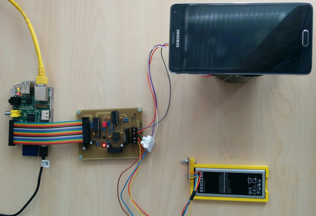
(a) Equipment for measuring energy consumption.

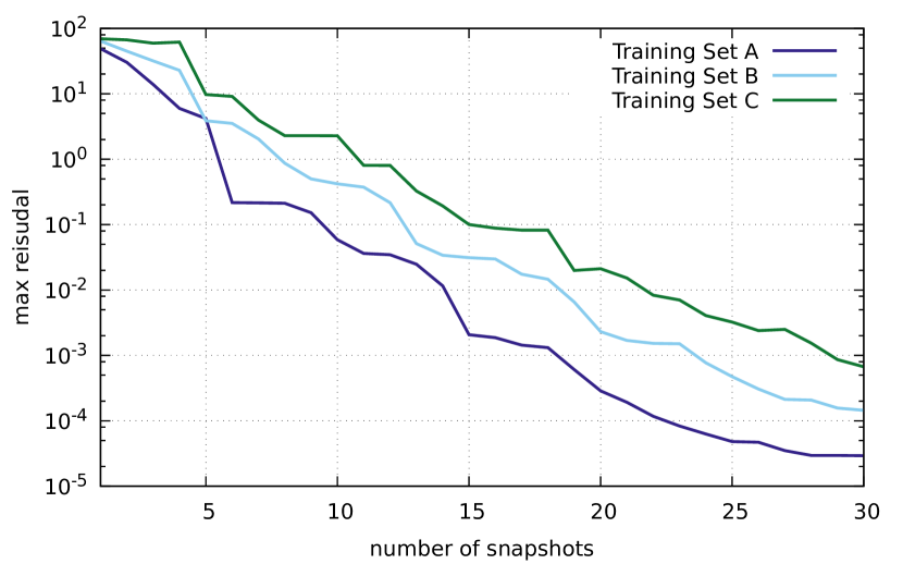
(b) Quality of the RBM with different number of snapshots.

Figure 10:

For the energy measurements, we used a custom measurement board with analog-to-digital converter connected to a Raspberry Pi. We designed a battery holder and battery replacement in order to perform energy measurements in situ. Figure 10(a) shows our energy evaluation setup. All energy measurement values in this section are absolute values taken from the Note 4 with fixed screen brightness. The power consumption of the device in idle mode was 0.4 W.

As simulation problem for the evaluation, we used the stationary diffusion-advection equation. This equation can be used to simulate the heat in an object as for the application for placing a hot tube as mentioned in the introduction. The equation has three parameters, one for the diffusion ($\mu_{\textit{diff}}$) and two for advection ($\mu_{\textit{advx}}$ and $\mu_{\textit{advy}}$). For the implementation, we discretized the equation using finite differences. As numerics library, we used the Apache Commons Maths library (version 3.6), which is the most popular Java numerics library, and NumPy (1.13.0) and SciPy (0.19.1), which provide hardware optimization on the server. Additionally to the pure Java implementation, we implemented the mobile-only approach natively using the Android Native Development Kit (NDK) and the Eigen C++ library in version 3.2.8.

9.2 Basis Generation Methods

Next, we evaluate the performance of the basis generation methods and how many snapshots are needed during query processing on the mobile device.

In order to quantify the number of snapshots needed to reach a certain quality, we created three different training sets $A$, $B$, and $C$. The training sets were chosen such that $A\subset B\subset C$, where parameters $\mu_{\textit{advx}}$ and $\mu_{\textit{advy}}$ spanned different parts of the parameter space expressing different behavior of the model ($[0,40]^{2}$ for $A$, $[-40,40]\times[0,40]$ for $B$, $[-40,40]^{2}$ for $C$). Parameter $\mu_{\textit{diff}}$ was for all three training sets in $[10,20]$. All intervals were discretized with step width $1.0$.

To quantify the relation between the size of the reduced basis and quality, we used the three training sets, executed the greedy basis generation algorithm (c.f. Section 2), and recorded the maximum residual of test sets. The test sets $A_{t},B_{t},C_{t}$ consist of $1000$ random points in the range of $A,B,C$. The discretization of the full problem was $256\times 256$, i.e. $256$ points in $x$ and $y$ direction.

In Fig. 10(b) depicts the relation between number of snapshots and quality for each training set. Training set $A$, which has smallest variation in the parameters, has the lowest maximum residual for a fixed number of snapshots. Notice that the residuum is measured in the Euclidean norm. To get a better impression, this norm is always bigger than the maximum absolute difference of any two points in the resulting vector. Therefore, a residual of, say $0.1$, means that the result multiplied by the problem matrix results in a vector which differs in all $256^{2}$ entries at most $0.1$ from the right-hand side. Therefore, for many practical applications, a basis with $10$, $15$, or $20$ snapshots would provide sufficient quality for this problem.

After evaluating the greedy basis generation and the basic approach, we now quantify the number of snapshots needed during online computation for different basis generation methods. The number of snapshots needed for the subspace approach and the reorder approach is dynamically depending on parameter $\mu$. We also want to quantify the fraction of snapshots typically needed for these approaches compared to the basic approach, which always uses all snapshots available in the reduced basis.

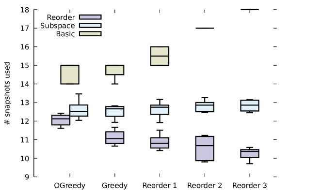
Figure 11: Mean number of snapshots needed in different approaches for different reduced basis generation methods. OGreedy is the orthogonal greedy basis. Reorder $k$ is the reorder basis generation method with $k$ additional snapshots.

Figure 11 depicts the number of snapshots needed for the reorder and the subspace approach in multiple basis generation runs. It also compares the greedy basis generation approach to our reorder basis generation approach. Using the reorder basis generation approach, the reorder approach performs better than using the greedy bases. In particular, for the reorder basis with $3$ additional the median mean number of snapshots for the reorder approach is 69.1 % lower than for the basic approach using an orthonormal greedy basis. On an orthonormal basis, the median mean number of snapshots of the subspace approach is only 83.5 % compared to the basic approach. Notice that for the reorder basis generation, the bigger $k$ is in the additional number of snapshots, the harder it is to generate the reduced basis because of numerical instabilities.

As these results suggest, we assume in the following that the subspace approach will only need 83.5 % of the snapshots and the reorder approach only 69.1% of the snapshots for the diffusion advection equation. Whenever we refer to the reorder approach, we assume that we use a reorder basis with $3$ additional snapshots.

9.3 Runtime

We compare the runtime of simulation runs for the different approaches on different mobile devices for both, single queries and multiple queries. Runtime of the adaptive approach can be split into runtime for the local case, when the available reduced basis provides sufficient quality, and runtime for the remote case, when the reduced basis needs an update from the server. The subspace approach was evaluated using $83.5\,\%$ of the snapshots. For each skipped snapshot, it had to compute the residual and the subspace. For the reorder approach, we assume that a reorder basis was generated and that the approach only needs 69.1 % of the snapshots. We included all computations for the overhead. For the mobile-approach, we used two implementations, one using pure Java and one using the Android Native Development Kit (NDK) in C++. We repeated the measurements for different discretizations of the underlying full simulation problem and for different numbers of snapshots.

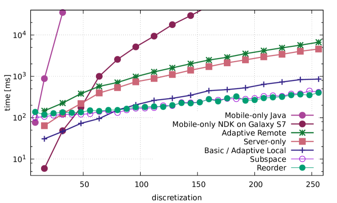
Figure 12: Runtime for varying problem discretizations.

Figure 12 depicts the average runtime for the processing of single queries for different sizes of the full problem. The full problem discretization is equidistant on both axes of the 2D domain. Therefore, for instance, for discretization $\mathcal{D}=32$, a matrix equation with a $32^{2}\times 32^{2}$ matrix has to be solved. The used reduced bases had $15$ snapshots. Most results from the Galaxy S7 were the same as for the Note 4. Only the performance of the mobile-only approach using the NDK was significantly better on the Galaxy S7. For simplicity, only the better results from the S7 are depicted. All other results depicted in Fig. 12 are from the Note 4. Results from the local case of the adaptive approach are very similar to results of the basic approach. Therefore, only the remote case of the adaptive approach is depicted. The server-only approach is over 280 times faster than the mobile-only approach in pure Java. The basic approach is again over 5 times faster than the server-only approach. The subspace approach is over $51\,\%$ faster than the basic approach. The reorder approach is only 3 % faster than the subspace approach. This is partly caused by the random access on the data file, which can be read as one big bulk operation in the subspace approach.

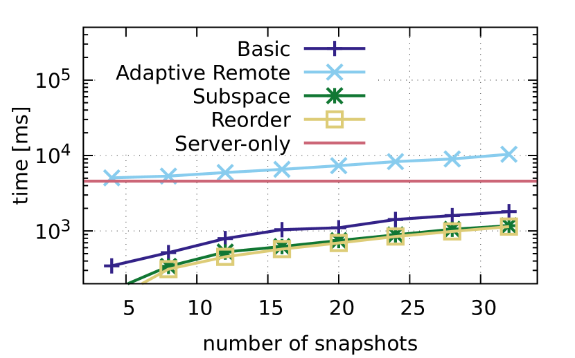
(a) Runtime for single queries with varying snapshot number.

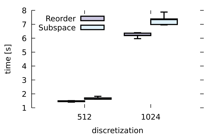
(b) Runtime for very high dimensions of 512 and 1024 with 15 snapshots.

Figure 13: Evaluation of the runtime.

As the improvement of the reorder approach until dimension $\mathcal{D}=256$ is not significant, we evaluated the subspace and the reorder approach for bigger reduced problems of dimension $\mathcal{D}=512$ and $\mathcal{D}=1024$. While for the previous evaluation, snapshots had sizes of up to 500 KB, for dimension $\mathcal{D}=1024$, one snapshot has 8 MB. Figure 13(b) depicts results of this evaluations, where the reorder approach is 10 % faster for dimension $\mathcal{D}=512$ and 16.5 % faster for dimension 1024 comparing the median execution times.

As both implementations of the mobile-only approach perform very poorly, we compare our approaches in the following only with the server-only approach.

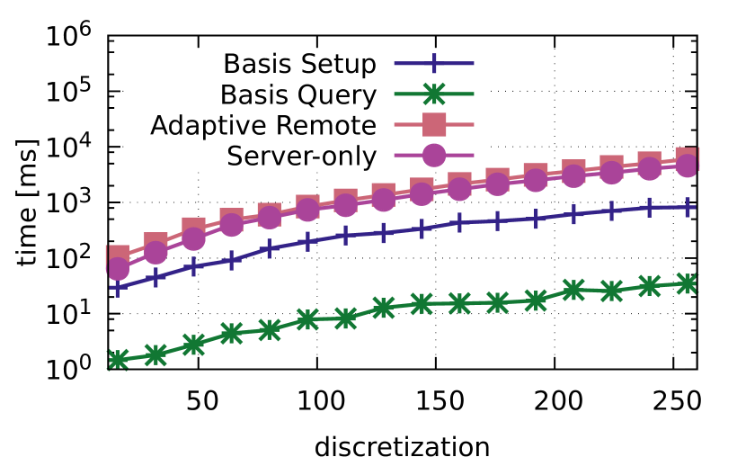
(a) Runtime for multiple queries with varying full problem dimension.

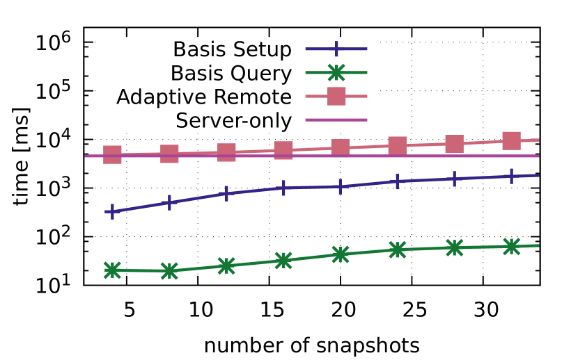
(b) Runtime for multiple queries with varying snapshots number.

Next, we compare the runtime for processing single queries with varying number of snapshots in the reduced basis. Figure 13(a) depicts the results with full problem dimension $\mathcal{D}=256$. As the server-only approach computes the full problem, it does not depend on the snapshot size. With growing number of snapshots, our approaches need more time. The speedup of the basic approach against the server-only approach is over $13.2$ for $4$ snapshots and decreases to $2.5$ for $32$ snapshots. However, with $64$ snapshots, the speedup of our approaches against the server-only approach is still above $1.3$ for the basic approach. The subspace approach is 45 % faster than the basic approach. As the reorder approach is only 2.8 % faster than the subspace approach, we see that the number of snapshots does not have too much impact on the performance of the reorder approach when snapshots are small.

Many applications need multiple queries, e.g., to continuously visualize simulation results for augmented reality. Our basic and adaptive approach can be split into a setup part, where the snapshots are loaded from internal storage, and a query part, where the solution for a parameter $\mu$ is computed. Figure 14(a) depicts the runtime for setup phase and processing of queries for different sizes of the full problem with $15$ snapshots and Fig. 14(b) for different number of snapshots with discretization $\mathcal{D}=256$. Both figures show that most time is needed for the setup phase. Processing queries even with $32$ snapshots and $\mathcal{D}=256$ only takes 63 ms. Query processing using the basic approach on the mobile device is over $131$ times faster than the server-only approach for $\mathcal{D}=256$ and $15$ snapshots.

9.4 Energy Consumption

Energy is a very important resource for battery-powered mobile devices. Therefore, we evaluated the energy consumption of all four approaches with varying full-problem discretization, as well as for varying number of snapshots.

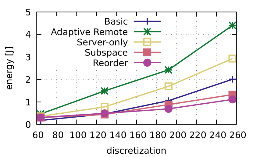
(a) Energy consumption for different discretizations of the full problem.

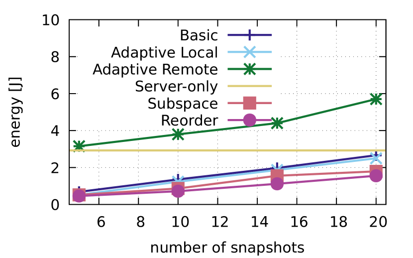
(b) Energy consumption for different number of snapshots.

Figure 15: Evaluation of the energy consumption.

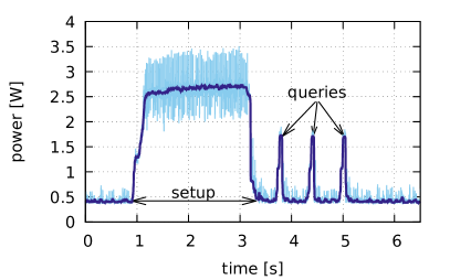
Figure 16: Energy consumption of the basic approach processing three queries after initial setup.

Figure 15(a) depicts the energy consumption for varying discretizations of the full problem. The initial bases had $15$ snapshots. Updates in the adaptive approach consume more energy than the server-only approach. The energy consumption of the local case of the adaptive approach is very similar to the basic approach. Both only need 68 % of energy compared to the server-only approach. The subspace approach needs 34 % of the energy of the basic approach, while the reorder approach saves another 18 % of energy compared to the subspace approach. The mobile-only approaches, which are not depicted, consume significantly more energy. The NDK version consumed 3.9 J for discretization $\mathcal{D}=32$ and over 84 J for $\mathcal{D}=64$. The pure Java implementation consumes more than 80 J for $\mathcal{D}=32$.

In addition to varying the discretization of the underlying full problem, we also evaluated the impact of the basis size on the energy consumption of our approaches. Figure 15(b) depicts the energy consumption for different numbers of snapshots with full problem size $D=256$. As already seen for the runtime, also the energy consumption increases for higher number of snapshots. The server-only and the mobile-only approaches are not affected by the number of snapshots.

Our approaches can reduce the energy consumption for single queries significantly, especially when the discretization of the full problem is high and the number of snapshots needed is low. The adaptive approach consumes lesser energy than the server-only approach, if more than $8\,\%$ of the queries can be answered locally for $\mathcal{D}=256$ and $5$ snapshots. If the snapshot size is increased to $15$, the adaptive approach is still beneficial if more than $58\,\%$ of the requests can be answered locally. The subspace approach saves over $32\,\%$ of energy compared to the basic approach with $20$ snapshots. In addition, the reorder approach saves another 13 % compared to the subspace approach.

We also considered the energy consumption for multiple queries for the basic and the adaptive approach. Figure 16 depicts the power during the setup phase and the queries for a basis with $64$ snapshots. Between the operations, the device was idle. Most energy is needed for reading the reduced basis from internal storage. After the basis is available in memory, processing one query only takes less than 0.17 J. For a basis with 15 snapshots and $\mathcal{D}=256$, the median energy consumption for one query was 0.04 J. This is 73 times less energy as for the server-only approach.

Overall, the evaluation showed that our approaches significantly improve latency and energy consumption especially for processing queries after the reduced basis is available in memory. In this case, the basic approach achieves a speedup of over 131 compared to the server-only approach. At the same time, it saves 73 times of the energy. For single queries, the subspace approach reduces the energy consumption in the setup phase and therefore needs 34 % lesser energy as the basic approach. Additionally, our reorder approach is able to save again 18% of energy compared to the subspace approach and over 62 % of energy compared to the server-only approach.

10 Related Work

In this section, we discuss work related to our approach. Related work can be categorized into approaches using the Reduced Basis Method (RBM), quality-aware approaches, and code-offloading approaches.

We are not the first to execute the RBM on constrained computing devices. Huynh et al. already proposed to use the RBM for deployment of thin computing platforms [5]. In this approach, the pre-computation of the reduced basis is executed prior to deployment, and the approximation using the reduced basis is executed after deployment. However, in contrast to our approaches, they do not consider the networking capabilities of the devices. Therefore, their approach is restricted to one single reduced basis that cannot be changed after the deployment. Especially when the parameter region of queries of the application changes over time, their approach is not able to provide approximate solutions with quality constraints, in contrast to our approach,

Recently, Pandey et al. proposed a mobile distributed framework for quality-aware applications [13]. Their approach adapts the quality of computations in order to achieve better resource efficiency of pervasive mobile applications. To this end, they construct workflows that reduce the quality of the application and meet the requirements of the user. However, we argue that numerical simulations need a more specific method such as the reduced basis method together with specific quality metrics like the residual.

The basic idea of approximate computing is to reduce the accuracy of calculations in favor of reduced energy consumption, runtime, less powerful hardware, etc. For instance, Xu et al. presented an approach in [14] that reduces the refresh rate of memory to save energy, which at the same time increases the probability of bit errors. A second example is the IMPACT system by Gupta et al. [15] that implements an imprecise adder for low-power approximate computing. Such hardware-centric solutions are complementary to our approach.

Code offloading is a generic method to offload compute-intensive code from the mobile device to a server infrastructure. Similar to our approach, code offloading tries to optimize energy efficiency and execution time of mobile applications. To this end, various offloading approaches have been proposed in the literature [16, 17, 18, 19, 20, 21, 22], which try to find an optimal partitioning of the application code into code executed locally on the mobile device or remotely. For instance, Cuervo et al. presented the MAUI system, which performs code offloading on a function-level in order to optimize for energy [16]. In this approach, the user has to annotate the code in order to mark functions that can be offloaded to the remote server. During compile time, the system creates proxies, which represent either local or remote execution. During runtime, the system continuously monitors the program and network characteristics and decides if the function should be called locally or remotely, depending on the energy characteristics of the device.

Since offloading is agnostic to the semantics of the application whose code is offloaded, it is not restricted to mobile simulations but can be used to optimize compute-intensive mobile applications in general. However, as a generic approach code offloading is not optimized for the specific properties of numeric simulations. In particular, it does not consider the quality of the simulation result and does not exploit the possibility to trade-off quality for energy efficiency as we do by using the Reduced Basis Method.

11 Conclusion & Future Work

In this paper, we presented a middleware for enabling complex numerical simulations on resource-constrained mobile devices by distributing the simulation between mobile device and a server infrastructure. Such a middleware is needed for interactive simulations in the field, e.g., an engineer using a head-mounted augmented reality device who wants to simulate the heat in an object to adjust its placement according to the surrounding materials. We presented four approaches for solving this problem using the Reduced Basis Method (RBM), which pre-computes a reduced representation of the simulation to reduce the evaluation time. The first approach was to pre-compute a reduced basis on the server and send this basis to the mobile device. In order to calculate an approximation of the simulation, no further communication is necessary. The second approach was more interactive and utilized the fast error indicator of the RBM. Using this indicator, the mobile device can efficiently check if the quality demands of the application are fulfilled. If the quality is not sufficient, the mobile device requests a basis update from the server. After such an update, the mobile device is able to answer queries with similar parameters completely autonomous without communication with the server. Goal of the third and fourth approach is to reduce the number of data to be read from internal storage, which we identified as major energy consumer. In addition, we also presented a novel approach for the pre-computation, which further reduces the data needed from internal storage during runtime.

We evaluated our approaches on real mobile devices in a real wireless network. We showed that our approach has lower energy consumption and is multiple times faster compared to two simple approaches. In particular, we showed that our approach, once it has performed a setup phase, is over 131 times faster and consumes 73 times less energy compared to offloading everything to a connected server. Still, our approach keeps quality requirements as requested and reports an error indicator to the user.

In the future, we will further extend our approach by integrating real time sensor data streams into the simulation.

Appendix A Error Estimation for the Reduced Basis Method

In simulations, the trade-off between accuracy and computational effort is made on many levels. One key property for serious simulation applications is to estimate or indicate the error. One important tool for error indication is the residual. The residual is the difference in an equation to be solved. For the RBM, the residual can be computed very fast, as essential parts can be pre-computed. As this is used in the adaptive and the subspace approach, we shortly sketch the procedure.

The RBM provides an approximation $Vu_{V}(\mu)$ for the solution $u(\mu)$ in the equation ${A(\mu)u(\mu)=f(\mu)}$ (c.f. Section 2). We can write this equation as $A(\mu)Vu_{V}(\mu)=f(\mu)+r$ with residual $r$. Using this equation, we can compute ${\lVert r\rVert^{2}=r^{T}r}$ as follows

$$\lVert\mathbf{r}\rVert^{2}=\ \mathbf{u}_{V}(\mu)^{T}\underbrace{\mathbf{V}^{T}\mathbf{A}(\mu)^{T}\mathbf{A}(\mu)\mathbf{V}}_{\mathbf{r}_{1}}\mathbf{u}_{V}(\mu)$$ (4a)

$$-\mathbf{u}_{V}(\mu)^{T}\underbrace{\mathbf{V}^{T}\mathbf{A}(\mu)^{T}\mathbf{f}(\mu)}_{\mathbf{r}_{2}}$$ (4b)

$$-\underbrace{\mathbf{f}(\mu)^{T}\mathbf{A}(\mu)\mathbf{V}}_{\mathbf{r}_{3}}\mathbf{u}_{V}(\mu)$$ (4c)

$$+\underbrace{\mathbf{f}(\mu)^{T}\mathbf{f}(\mu)}_{r_{4}}.$$ (4d)

Notice that $r_{1}$ to $r_{4}$ can be expressed as separable matrices. These matrices can be pre-computed after the basis construction. Also notice that a new snapshot will increase the matrix $V$ by exactly one column vector. Therefore, this will only add columns and rows to the matrices $r_{1}$ to $r_{4}$. Analogously, the last snapshot can be removed from the residual computation by trimming the matrices as needed for the subspace approach.

References

- [1] C. Dibak, B. Koldehofe, Towards Quality-aware Simulations on Mobile Devices, in: Informatik 2014, Gesellschaft für Informatik (GI), 2014.
- [2] C. Dibak, F. Dürr, K. Rothermel, Numerical Analysis of Complex Physical Systems on Networked Mobile Devices, in: MASS, IEEE, 2015. doi:10.1109/MASS.2015.12.
- [3] C. Dibak, F. Dürr, K. Rothermel, Demo: Server-assisted interactive mobile simulations for pervasive applications, in: PerCom Workshops, 2017. doi:10.1109/PERCOMW.2017.7917525.
- [4] J. Ware, N. Roy, An analysis of wind field estimation and exploitation for quadrotor flight in the urban canopy layer, in: ICRA, IEEE, 2016, pp. 1507–1514. doi:10.1109/ICRA.2016.7487287.
- [5] D. Huynh, D. Knezevic, J. Peterson, A. Patera, High-fidelity real-time simulation on deployed platforms, Computers & Fluids 43, symposium on High Accuracy Flow Simulations. doi:10.1016/j.compfluid.2010.07.007.
- [6] C. Dibak, A. Schmidt, F. Dürr, B. Haasdonk, K. Rothermel, Server-assisted interactive mobile simulations for pervasive applications, in: PerCom, IEEE, 2017. doi:10.1109/PERCOM.2017.7917857.
- [7] A. T. Patera, G. Rozza, Reduced basis approximation and a posteriori error estimation for parametrized partial differential equations, version 1.0, Copyright MIT 2006, to appear in (tentative rubric) MIT Pappalardo Graduate Monographs in Mechanical Engineering (2007).
- [8] B. Haasdonk, M. Ohlberger, Efficient reduced models and a posteriori error estimation for parametrized dynamical systems by offline/online decomposition, Mathematical and Computer Modelling of Dynamical Systems 17 (2) (2011) 145–161. doi:10.1080/13873954.2010.514703.
- [9] B. Haasdonk, Reduced basis methods for parametrized PDEs – a tutorial introduction for stationary and instationary problems, Chapter in P. Benner, A. Cohen, M. Ohlberger and K. Willcox: ”Model Reduction and Approximation for Complex Systems”, SIAM, Philadelphia (2016).
- [10] M. Barrault, Y. Maday, N. C. Nguyen, A. T. Patera, An ’empirical interpolation’ method: application to efficient reduced-basis discretization of partial differential equations, Comptes Rendus Mathematique 339 (9) (2004) 667–672. doi:10.1016/j.crma.2004.08.006.
- [11] K. Veroy, C. Prud’Homme, D. V. Rovas, A. T. Patera, A posteriori error bounds for reduced-basis approximation of parametrized noncoercive and nonlinear elliptic partial differential equations, in: Proceedings of the 16th AIAA computational fluid dynamics conference, Vol. 3847, Orlando, Florida, 2003, pp. 23–26. doi:10.2514/6.2003-3847.
-
[12]
G. Rozza, D. B. P. Huynh, A. T. Patera,
Reduced basis approximation
and a posteriori error estimation for affinely parametrized elliptic coercive
partial differential equations, Archives of Computational Methods in
Engineering 15 (3) (2008) 229.
doi:10.1007/s11831-008-9019-9.
URL https://doi.org/10.1007/s11831-008-9019-9 - [13] P. Pandey, D. Pompili, Mobidic: Exploiting the untapped potential of mobile distributed computing via approximation, in: 2016 IEEE International Conference on Pervasive Computing and Communications (PerCom), 2016, pp. 1–9. doi:10.1109/PERCOM.2016.7456515.
- [14] Q. Xu, T. Mytkowicz, N. Kim, Approximate computing: A survey, Design & Test, IEEE 33 (1) (2016) 8–22. doi:10.1109/MDAT.2015.2505723.
- [15] V. Gupta, D. Mohapatra, S. P. Park, A. Raghunathan, K. Roy, Impact: Imprecise adders for low-power approximate computing, in: ISLPED, IEEE, 2011.
- [16] E. Cuervo, A. Balasubramanian, D.-k. Cho, A. Wolman, S. Saroiu, R. Chandra, P. Bahl, Maui: making smartphones last longer with code offload, in: MobiSys, ACM, 2010. doi:10.1145/1814433.1814441.
- [17] S. Kosta, A. Aucinas, P. Hui, R. Mortier, X. Zhang, Thinkair: Dynamic resource allocation and parallel execution in the cloud for mobile code offloading, in: INFOCOM, IEEE, IEEE, 2012.
- [18] S. Yang, Y. Kwon, Y. Cho, H. Yi, D. Kwon, J. Youn, Y. Paek, Fast dynamic execution offloading for efficient mobile cloud computing, in: PerCom, 2013. doi:10.1109/PerCom.2013.6526710.
- [19] F. Berg, F. Dürr, K. Rothermel, Optimal predictive code offloading, in: MobiQuitous, ICST, 2014. doi:10.4108/icst.mobiquitous.2014.258023.
- [20] F. Berg, F. Dürr, K. Rothermel, in: WiMob, IEEE, 2015. doi:10.1109/WiMOB.2015.7348013.
- [21] Y. Zhang, D. Niyato, P. Wang, Offloading in mobile cloudlet systems with intermittent connectivity, Transactions on Mobile Computingdoi:10.1109/TMC.2015.2405539.
- [22] F. Berg, F. Dürr, K. Rothermel, Increasing the Efficiency of Code Offloading in n-tier Environments with Code Bubbling, in: MobiQuitous, IEEE, 2016. doi:10.1145/2994374.2994375.