The Eigenvalues Slicing Library (EVSL): Algorithms, Implementation, and Software

Abstract

This paper describes a software package called EVSL (for EigenValues Slicing Library) for solving large sparse real symmetric standard and generalized eigenvalue problems. As its name indicates, the package exploits spectrum slicing, a strategy that consists of dividing the spectrum into a number of subintervals and extracting eigenpairs from each subinterval independently. In order to enable such a strategy, the methods implemented in EVSL rely on a quick calculation of the spectral density of a given matrix, or a matrix pair. What distinguishes EVSL from other currently available packages is that EVSL relies entirely on filtering techniques. Polynomial and rational filtering are both implemented and are coupled with Krylov subspace methods and the subspace iteration algorithm. On the implementation side, the package offers interfaces for various scenarios including matrix-free modes, whereby the user can supply his/her own functions to perform matrix-vector operations or to solve sparse linear systems. The paper describes the algorithms in EVSL, provides details on their implementations, and discusses performance issues for the various methods.

1 Introduction

A good number of software packages have been developed in the past two decades for solving large sparse symmetric eigenvalue problems see, e.g., [5, 6, 7, 20, 26, 47, 35]. In most cases, these packages deal with the situation where a relatively small number of eigenvalues are sought on either end of the spectrum. Computing eigenvalues located well inside the spectrum is often supported by providing options in the software that enable one to exploit spectral transformations, i.e., shift-and-invert strategies [38]. However, these packages are generally not designed for handling the situation when a large number of these eigenvalues, reaching in the thousands or tens of thousands, are sought and when, in addition, they are located at the interior of the spectrum. Yet, it is now this breed of difficult problems that is often encountered in modern applications. For example, in electronic structure calculations, a method such as Density Functional Theory (DFT) will see the number of ground states increase to very large numbers in realistic simulations. As an illustration, the 2011 Gordon Bell winning paper [25] showed a calculation on the K-computer that had as many as 107,292 atoms leading to the computation of 229,824 orbitals (eigenvectors of the Kohn-Sham equation). In the introduction of the same paper the authors pointed out that “in order to represent actual behavior of genuine materials, much more computational resources, i.e., more CPU cycles and a larger storage volume, are needed to make simulations of up to 100,000 atoms.” As a side note, it is worth mentioning that the article discusses how the orbitals were divided in 3 sets of 76,608 orbitals handled in parallel, a perfect example of spectrum slicing. In computations related to excited states, e.g., with the Time-dependent Density Functional Theory (TDFT) approach, the situation gets much worse [8] since one needs to compute eigenvalues that are not only related to occupied states but also those associated with a sizable number of unoccupied ones. EVSL is specifically designed to tackle these challenges and to address standard and generalized symmetric eigenvalue problems, encountered in large scale applications of the type just discussed.

As a background we will begin with a brief review of the main software packages currently available for large eigenvalue problems, noting that it is beyond the scope of this paper to provide an exhaustive survey. We mentioned earlier that most of the packages that are available today aim at extracting a few eigenvalues. Among these, the best known is undoubtedly ARPACK which has now become a de-facto standard for solvers that rely on matrix-vector operations. ARPACK uses the Implicitly Restarted Arnoldi Method for the non-symmetric case, and Implicitly Restarted Lanczos Method for the symmetric case [35]. ARPACK supports various types of matrices, including single and double precision real arithmetic for symmetric and non-symmetric cases, and single and double precision complex arithmetic for standard and generalized problems. In addition, ARPACK can also calculate the Singular Value Decomposition (SVD) of a matrix. Due to the widespread use of ARPACK, once development stalled, vendors began creating their own additions to ARPACK, fracturing what used to be a uniform standard. ARPACK-NG was created as a joint project between Debian, Octave and Scilab, in an effort to contain this split.

To cope with the large memory requirements required by the use of the (standard) Lanczos, Arnoldi and Davidson methods, restart versions were developed that allowed to reuse previous information from the Krylov subspace in clever ways. Thus, TRLan [54, 53] was developed as a restarting variant of the Lanczos algorithm. It uses the thick-restart Lanczos method [48], whose generic version is mathematically equivalent to the implicitly restarted Lanczos (IRL) method. The TRLan implementation supports both single address memory space and distributed computations [60, 55] and also supports user provided matrix-vector product functions. More recently, TRLan was rewritten in C as the $\alpha$-TRLAN package, which has an added feature of adaptively selecting the subspace dimensions [60].

As part of the Trilinos project [16], Anasazi provides an abstract framework to solve eigenvalue problems, enabling the user to choose or provide their own functions [6]. It utilizes advanced paradigms such as object-oriented programming and polymorphism in C++, to enable a robust and easily expandable framework. With the help of abstract interfaces, it lets users combine and create software in a modular fashion, allowing them to construct a precise setup needed for their specific problem. A notable recent addition to Anasazi is the TraceMin eigensolver [43, 27, 44], which can be viewed as a predecessor of the Jacobi-Davidson algorithm [21].

The BLOPEX package [30] is available as part of the Hypre library [19], and also as an external package to PETSc [28]. Through this integration, BLOPEX is able to make use of pre-existing highly optimized preconditioners. BLOPEX uses the Locally Optimal Block Preconditioned Conjugate Gradient method (LOBPCG) [29], which can be combined with a user-provided preconditioner. It is aimed at computing a few extreme eigenvalues of symmetric positive generalized eigenproblems, and supports distributed computations via the message passing interface (MPI).

SLEPc [26] is a package aimed at providing users with the ability to use a variety of eigensolvers to solve different types of eigenvalue problems. SLEPc, which is integrated into PETSc, supports quite a few eigensolvers, with the ability to solve SVD problems, Polynomial Eigenvalue problems, standard and generalized problems, and it also allows solving interior eigenvalue problems with shift-and-invert transformations. SLEPc is written in a mixture of C, C++, and Fortran, and can be run in parallel on many different platforms.

PRIMME [47] is a relatively recent software package that aims to be a robust, flexible and efficient, ‘no-shortcuts’ eigensolver. It includes a multilevel interface, that allows both experts and novice users to feel at ease. PRIMME uses nearly optimal restarting via thick restart and ‘+k restart’ to minimize the cost of restarting. By utilizing dynamic switching between methods it is able to achieve accurate results very quickly [47]. The interesting article [51] shows a (limited) comparison of a few software packages and found the GD+K algorithm from PRIMME to be the best in terms of speed and robustness for the problems they considered. These problems originate from quantum dot and quantum wire simulations in which the potential is given and, to paraphrase the authors, ‘restricts the computation to only a small number of interior eigenstates from which optical and electronic properties can be determined’. In fact, the goal is to compute the two eigenvalues that define valence and conduction bands. There may be thousands of eigenvalues to the left of these two eigenvalues and the paper illustrates how some codes, e.g., the IRL routine from ARPACK faces severe difficulties in this case because they are designed for computing smallest (or largest) eigenvalues.

While the packages mentioned above are used to calculate a limited number of eigenvalues, the FILTLAN [20], and FEAST [39] packages are, like EVSL, designed to compute a large number of eigenpairs associated with eigenvalues not necessarily located at the extremity of the spectrum. Rather than resort to traditional shift-invert methods, FILTLAN uses a combination of (non-restarted) Lanczos and polynomial filtering with Krylov projection methods to calculate both the interior and extreme eigenvalues. In addition, it uses the Lanczos algorithm and partial reorthogonalization to improve performance [20]. FEAST has been designed with the same motivation as EVSL, namely to solve the kind of eigenvalue problems that are prevalent in solid state physics. It can search for an arbitrary number of eigenvalues of Hermitian and non-Hermitian eigenvalue problems. Written in Fortran, it exploits the well-known Cauchy integral formula to express the eigenprojector. This formula is approximated via numerical integration and this leads to a rational filter to which subspace iteration is applied. Single node and multi-node versions are available via OpenMP and MPI. The idea of using Cauchy integral formulas has also been exploited by Sakurai and co-authors [41, 42, 4]. A related software package called z-Pares [18] has been made available from the University of Tsukuba, which is implemented in Fortran 90/95 and supports single and double precision. It offers interfaces for both sparse and dense matrices but also allows arbitrary matrix-vector products via reverse communication. This code was developed with a high degree of parallelism in mind and, for example, it can utilize a 2-level distributed parallelism via a pair of MPI communicators.

A number of other packages implement specific classes of methods. Among these is JADAMILU [7] which focuses on the Jacobi-Davidson framework to which it adds a battery of preconditioners. It too is geared toward the computation of a few selected eigenvalues. The above list is by no means exhaustive and the field is constantly evolving. What is also interesting to note is that these packages are rarely used in applications such as the ones mentioned above where a very large number of eigenvalues are computed. Instead, most application packages, including PARSEC [32], CASTEP [46], ABINIT [24], Quantum Expresso [17], OCTOPUS [2], and VASP [31] implement their own eigensolvers, or other optimization schemes that bypass eigenvalue problems altogether. For example, PARSEC implements a form of nonlinear subspace iteration accelerated by Chebyshev polynomials. In light of this it may be argued that efforts to develop general purpose software to tackle this class of problems may be futile. The counter-argument is that even if a small subset from a package, or a specific technique from it, is adapted or retrofitted into the application, instead of the package being entirely adopted, the effort will be worthwhile if it leads to significant gains.

We end this section by introducing our notation and the terminology used throughout the paper. The generalized symmetric eigenvalue problem (GSEP) considered is of the form:

$$Ax=\lambda Bx,$$ (1)

where both $A$ and $B$ are $n$-by-$n$ large and sparse real symmetric and $B$ is positive definite. When $B=I$, (1) reduces to the standard real symmetric eigenvalue problem (SEP)

$$Ax=\lambda x.$$ (2)

For generalized eigenvalue problems we will often refer to the Cholesky factor $L$ of $B$ which satisfies $B=LL^{T}$, where $L$ is lower triangular. We will also refer to $B^{1/2}$ the matrix square root of $B$. It is often the case that $L$ is expensive to compute, e.g., for problems that arise from 3-D simulations. In this cases, we may utilize the factorization $B=B^{1/2}\cdot B^{1/2}$ and approximate the action of $B^{1/2}$ by that of a low degree polynomial in $B$. If the smallest eigenvalue is $\lambda_{min}$ and the largest $\lambda_{max}$, we refer to the interval $[\lambda_{min},\ \lambda_{max}]$ as the spectral interval. We will often use this term for an interval $[a,\ b]$ that tightly includes $[\lambda_{min},\ \lambda_{max}]$.

2 Methodology

This section begins with an outline of the methodologies of the spectrum slicing algorithms as well as the projection methods for eigenvalue problems that have been implemented in EVSL. For further reading, the theoretical and algorithmic details can be found in [36, 57, 58].

2.1 Spectrum slicing

The EVSL package relies on a spectrum slicing approach to deal with the computation of a very large number of eigenvalues. The idea of spectrum slicing consists of a divide-and-conquer strategy: the target interval $[\xi,\eta]$ that contains many eigenvalues is subdivided into a number of subintervals and the eigenvalues from each subinterval are then computed independently from the others. The simplest slicing method would be to divide $[\xi,\eta]$ uniformly into equal size subintervals. However, when the distribution of eigenvalues is highly nonuniform, some subintervals may contain many more eigenvalues than others and this will cause a severe imbalance in the computational time and, especially, in memory usage. EVSL adopts a more sophisticated slicing strategy based on exploiting the spectral density that is also known density of states (DOS). The spectral density is a function $\phi(t)$ of real number $t$ that provides for any given $t$ a probability measure for finding eigenvalues near $t$. Specifically, $n\phi(t)\Delta t$ will give an approximate number of eigenvalues in an infinitesimal interval surrounding $t$ and of width $\Delta t$. For details, see, e.g., [37]. Formally, the DOS for a Hermitian matrix $A$ is defined as follows:

$$\phi(t)=\frac{1}{n}\sum_{j=1}^{n}\delta(t-\lambda_{j}),$$ (3)

where $\delta$ is the Dirac $\delta$-function or the Dirac distribution, and the $\lambda_{j}$’s are the eigenvalues of $A$ or $B^{-1}A$. Written in this formal form, the DOS is not a proper function but a distribution and it is its approximation by a smooth function that is of interest [37]. Notice that if the DOS function $\phi$ were available, the exact number of eigenvalues located inside $[\xi,\eta]$ could be obtained from the integral

$$\int_{\xi}^{\eta}n\phi(t)dt=\int_{\xi}^{\eta}\sum_{j}\delta(t-\lambda_{j})dt.$$

Thus, the task of slicing $[\xi,\eta]$ into $n_{s}$ subintervals that roughly contain the same number of eigenvalues can be accomplished by ensuring that the integral of $\phi$ on each subinterval is an equal share of the integral on the whole interval, i.e,

$$\int_{t_{i}}^{t_{i+1}}\phi(t)dt=\frac{1}{n_{s}}\int_{\xi}^{\eta}\phi(t)dt,\quad i=0,1,\ldots,n_{s}-1,$$ (4)

where $[t_{i},t_{i+1}]$ denotes each subinterval with $t_{0}=\xi$ and $t_{n_{s}}=\eta$. The values of the endpoints $\{t_{i}\}$ can be computed easily by first finely discretizing $[\xi,\eta]$ with $N\gg n_{s}$ evenly spaced points $x_{0}=\xi\!<\!x_{1}\!<\!\ldots\!<\!x_{N-2}\!<\!x_{N-1}=\eta$ and then placing each $t_{i}$ at some $x_{j}$ such that (4) can be fulfilled approximately. Figure 1 shows an illustration of spectrum slicing with DOS.

Clearly, the exact DOS function $\phi$ is not available since it requires the knowledge of the eigenvalues which are unknown. However, there are inexpensive procedures that provide an approximate DOS function $\tilde{\phi}$, with which reasonably well-balanced slices can usually be obtained. Two types of methods have been developed for computing $\tilde{\phi}$. The first method is based on the kernel polynomial method (KPM), see, e.g., [37] and the references therein, and the second one uses a Lanczos procedure and the related Gaussian quadrature [57]. These two methods are in general computationally inexpensive relative to computing the eigenvalues and require the matrix $A$ only through matrix-vector operations.

The above methods for computing DOS can be extended to generalized eigenvalue problems, $Ax=\lambda Bx$. In addition to the matrix-vector products with $A$, these methods require solving systems with $B$, and also with $B^{1/2}$ or with $L^{\mathsf{T}}$ where $L$ is the Cholesky factor of $B$, to generate a correct starting vector. A canonical way to do this is to obtain the Cholesky factor via a sparse direct method. This may sometimes be too expensive whereas in many applications that arise from finite element discretization, where $B$ is a very well conditioned mass matrix, using iterative methods such as Chebyshev iterations or the least-squares polynomial approximation discussed in [57] can become a much more attractive alternative.

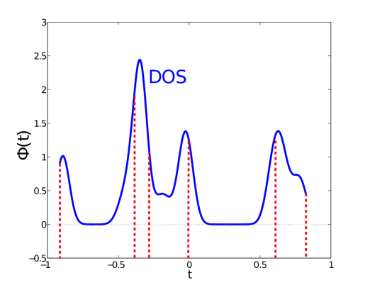
Fig. 1: An illustration of slicing a spectrum into $5$ subintervals $[t_{i},t_{i+1}]$ $(i=0,\ldots,5)$. The solid blue curve represents a smoothed DOS and the dotted red lines separate the subintervals.

2.2 Filtering techniques

An effective strategy for extracting eigenvalues from an interval $[t_{i},t_{i+1}]$ that is deep inside the spectrum, is to apply a projection method on a filtered matrix, where a filter function $\rho(t)$ aims at amplifying the desired eigenvalues located inside $[t_{i},t_{i+1}]$ and dampening those outside $[t_{i},t_{i+1}]$. This is also referred to as spectral transformation and it can be achieved via a polynomial filter or a rational one. Both types of filtering techniques have been developed and implemented in EVSL, with a goal of providing different effective options for different scenarios. The main goal of a filter function is to map the wanted part of the spectrum of the original matrix to the largest eigenvalues of the filtered matrix. Figure 2 illustrates a polynomial filter for the interval $[0,0.3]$.

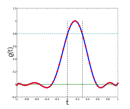
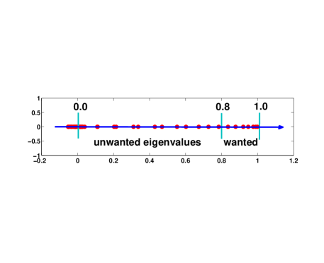
Fig. 2: An illustration of filtering techniques for real symmetric eigenvalue problems. Left: The eigenvalues inside $[-1,1]$ are mapped to the eigenvalues of the filtered matrix, which are the red dotted points along the blue solid curve. Right: The spectrum of the filtered matrix, where the wanted eigenvalues in $[0,0.3]$ are mapped into the largest ones of the filtered matrix. In this case the filter has been built so that these transformed eigenvalues are larger than $0.8$.

2.2.1 Polynomial filtering

The polynomial filter adopted in EVSL is constructed through a Chebyshev polynomial expansion of the Dirac delta function based at some well-selected point inside the target interval. Since Chebyshev polynomials are defined over the interval $[-1,\ 1]$, a linear transformation is needed to map the eigenvalues of $B^{-1}A$ onto this interval. This is achieved by applying a simple linear transformation:

$$\widehat{A}=\frac{A-cB}{d}\qquad\mbox{with}\quad c=\frac{\lambda_{\max}+\lambda_{\min}}{2}\quad\mbox{and}\quad d=\frac{\lambda_{\max}-\lambda_{\min}}{2},$$ (5)

where $\lambda_{\max}$ and $\lambda_{\min}$ are the largest and smallest eigenvalues of $B^{-1}A$, respectively. These two extreme eigenvalues can be efficiently estimated by performing a few steps of the Lanczos algorithm. Similarly, the target interval $[t_{i},t_{i+1}]$ should be transformed into $[\hat{t}_{i},\hat{t}_{i+1}]\equiv[(t_{i}-c)/d,(t_{i+1}-c)/d]$. Let $T_{j}(t)$ denote the Chebyshev polynomial of the first kind of degree $j$. The $k$-th degree polynomial filter function $\rho(t)$ for interval $[\hat{t}_{i},\hat{t}_{i+1}]$ centered at $\gamma$ takes the form

$$\rho(t)=\frac{\sum_{j=0}^{k}\mu_{j}T_{j}(t)}{\sum_{j=0}^{k}\mu_{j}T_{j}(\gamma)},$$ (6)

where the expansion coefficients are

$$\mu_{j}=\begin{cases}\frac{1}{2}&\mbox{if}\ j=0\\ \cos(j\cos^{-1}(\gamma))&\mbox{otherwise}\end{cases}\quad.$$ (7)

Notice that the filter function $\rho(t)$ only contains two parameters: the degree $k$ and the center $\gamma$, which are determined as follows. From a lowest degree (which is $2$), we keep increasing $k$ until the values $\rho(\hat{t}_{i})$ and $\rho(\hat{t}_{i+1})$ at the boundary of the interval are less than or equal to a predefined threshold $\tau$, where by default $\tau=0.8$ and we have $\rho(\gamma)=1$ by construction. For any degree $k$ that is attempted, the first task is to select $\gamma$ so that the filter is “balanced” such that its values at the ends of the interval are the same, i.e., $\rho(\hat{t}_{i})=\rho(\hat{t}_{i+1})$. This can be achieved by applying Newton’s method to solve the equation

$$\rho(\hat{t}_{j})-\rho(\hat{t}_{j+1})=0,$$ (8)

where the unknown is $\gamma$. If $\rho(\hat{t}_{i})$ and $\rho(\hat{t}_{i+1})$ do not exceed $\tau$, the selection procedure terminates and returns the current polynomial of degree $k$. Otherwise $k$ is increased and the procedure will be repeated until a maximum allowed degree is reached. There are situations that very small intervals require a degree of a few thousands.

In order to reduce the oscillations near the boundaries of the interval, it is customary to introduce damping multipliers to $\mu_{j}$. Several damping approaches are available in EVSL, where the default Lanczos $\sigma$-damping [33, Chap. 4] is given by

$$\hat{\mu}_{j}=\sigma_{j}^{k}\mu_{j},$$ (9)

with

$$\sigma_{j}^{k}=\begin{cases}1&\mbox{if}\ j=0\\ \frac{\sin(j\theta_{k})}{j\theta_{k}},\quad\theta_{k}=\frac{\pi}{k+1}&\mbox{otherwise}\end{cases}\quad.$$

An illustration of two polynomial filters with and without the Lanczos $\sigma$-damping is given Figure 3, which clearly shows the effect of damping factors for annihilating oscillations. For additional details on selecting the degree, the balancing procedure, and damping oscillations of the polynomial filter, we refer to our earlier paper [36].

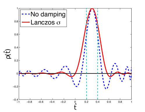
Fig. 3: Polynomial filters of degree 16 with the Lanczos $\sigma$-damping and without damping for interval $[0.2,0.4]$.

2.2.2 Rational filtering

The second type of filtering techniques in EVSL is rational filtering, which can be a better alternative to polynomial filtering in some cases. Traditional rational filter functions are usually built from the Cauchy integral representation of the step function $h_{[t_{j},\ t_{j+1}]}$. Formally, the Cauchy integral of the resolvent yields a spectral projector associated with the eigenvalues inside the interval $[t_{j},t_{j+1}]$. A good approximation of this projector can be obtained by employing a numerical quadrature rule. Thus, the step function is approximated as follows:

$$h_{[t_{j},t_{j+1}]}=\frac{1}{2\pi i}\int_{\Gamma}\frac{1}{s-z}ds\approx\sum_{j=1}^{2p}\frac{\alpha_{j}}{(z-\sigma_{j})}=\rho(z),$$ (10)

where $\Gamma$ denotes a circle centered at $(t_{j}+t_{j+1})/2$ with radius $(t_{j+1}-t_{j})/2$. The poles $\sigma_{j}\in\mathbb{C}$ are taken as the quadrature nodes along $\Gamma$ and $\alpha_{j}$ are the expansion coefficients. EVSL implements both Cauchy integral-based rational filters and the more flexible least-squares (L-S) rational filters discussed in [58]. In general, a L-S rational filter takes the following form:

$$\rho(z)=\sum_{j=1}^{2p}\sum_{k=1}^{k_{j}}\frac{\alpha_{jk}}{(z-\sigma_{j})^{k}},$$ (11)

where pole $\sigma_{j}$ is repeated $k_{j}$ times with the aim of reducing the number of poles on one the hand and improving the quality of the filter for extracting eigenvalues on the other. In particular, if $\sigma_{i}$ is equal to the conjugate of $\sigma_{i+p}$, (11) can be simplified as

$$\rho(z)=2\Re e\sum_{j=1}^{p}\sum_{k=1}^{k_{j}}\frac{\alpha_{jk}}{(z-\sigma_{j})^{k}}.$$ (12)

In its current implementation, the procedure for constructing the L-S rational filter starts by choosing the quadrature nodes, i.e., the poles $\sigma_{j}$. Once the $\sigma_{j}$’s are selected, the coefficients $\alpha_{jk}$ can be computed by solving the following problem

$$\min\left\|h_{[t_{j},t_{j+1}]}-\rho(z)\right\|_{w}^{2},$$ (13)

where the norm is associated with the standard $L_{2}$ inner product

$$\left\langle f,g\right\rangle=\int_{-\infty}^{\infty}w(t)f(t)\overline{g(t)}dt,$$ (14)

and the weight function $w(t)$ is taken to be of the form

$$w(t)=\begin{cases}0.01&\mbox{if}\quad t_{j}\leq t\leq t_{j+1}\\ 1&\mbox{otherwise}\end{cases}\quad.$$ (15)

Since it is desirable to have the same fixed value $1/2$ at the boundaries as for the Cauchy integral filters, the L-S rational filter (12) is scaled by $2\rho(t_{j})$.

The left panel of Figure 4 shows a comparison of a L-S rational filter and two Cauchy integral rational filters for the interval $[-1,1]$ both using $p=3$ poles. The Cauchy integral rational filters are constructed by applying the Gauss Legendre rule and the mid-point rule to discretize (10), whereas the L-S rational filter is computed with the same poles and the coefficients are computed by solving (13). In this example, the L-S rational filter achieves almost the same damping effect as the Gauss Legendre filter but unlike the other two rational filters, it does not approximate the step function and amplifies the wanted eigenvalues to much higher values. The right panel shows three L-S rational filters constructed by repeating only $1$ pole located at $\sigma_{1}=i$ (where $i$ is the imaginary unit) for $k$ times. It shows that the L-S rational filters decay faster across the boundaries as the value of $k$ increases.

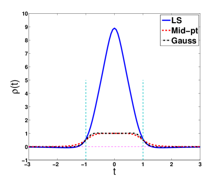
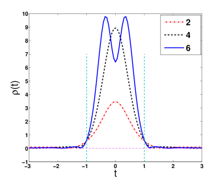
Fig. 4: Left: Comparison of a least-squares rational filter and two Cauchy integral filters using the Gaussian Legendre rule and the mid-point rule with $p=3$. The L-S rational filter uses the same poles as the Gaussian Legendre filter. Right: Comparison of L-S rational filters obtained from repeating one pole located at $(0,1)$ $k$ times, where $k=2,4,6$.

2.3 Lanczos algorithms for standard eigenvalue problems

For a symmetric matrix $A$, the Lanczos algorithm builds an orthonormal basis of the Krylov subspace

$$\mathcal{K}_{m}:=\mathrm{span}\{q_{1},Aq_{1},\ldots,A^{m-1}q_{1}\},$$

where, at step $j$, the vector $Aq_{j}$ is orthonormalized against $q_{j}$ and $q_{j-1}$ when $j>1$.

$$\beta_{i+1}q_{i+1}=Aq_{i}-\alpha_{i}q_{i}-\beta_{i}q_{i-1}.$$ (16)

In exact arithmetic, the 3-term recurrence would deliver an orthonormal basis of the Krylov subspace $K_{m}$ but in the presence of rounding, orthogonality between the $q_{i}$’s is quickly lost, and a form of reorthogonalization is needed in practice. EVSL uses full reorthogonalization to enforce the orthogonality to working precision, which is performed by no more than two steps of the classical Gram-Schmidt algorithm [22, 23] with the DGKS correction [10]. Let $T_{m}$ denote the symmetric tridiagonal matrix

$$T_{m}=\mbox{tridiag}(\beta_{i},\alpha_{i},\beta_{i+1}),$$ (17)

where $\alpha_{i},\beta_{i}$ are from (16) and define $Q_{m}=[q_{1},q_{2},\ldots,q_{m}]$. Let $(\theta_{i},y_{i})$ be an eigenpair of $T_{m}$. It is well-known that the Ritz values and vectors $(\theta_{i},Q_{m}y_{i})$ can provide good approximations to extreme eigenvalues and vectors of $A$ with a fairly small value of $m$. EVSL adopts a simple non-restart Lanczos algorithm and a thick-restart (TR) Lanczos algorithm [49, 55] as they blend quite naturally with the filtering approaches. In addition to TR, another essential ingredient is the inclusion of a “locking” mechanism, which consists of an explicit deflation procedure for the converged Ritz vectors.

2.4 Lanczos algorithms for generalized eigenvalue problems

A straightforward way to extend the approaches developed for standard eigenvalue problems to generalized eigenvalue problems is to transform them into the standard form. Suppose the Cholesky factorization $B=LL^{\mathsf{T}}$ is available, problem (1) can be rewritten as

$$L^{-1}AL^{-\mathsf{T}}y=\lambda y,\quad\mbox{with}\quad y=L^{\mathsf{T}}x,$$ (18)

which takes the standard form with the symmetric matrix $L^{-1}AL^{-\mathsf{T}}$. The matrix $L^{-1}AL^{-\mathsf{T}}$ does not need to be formed explicitly, since the procedures discussed above utilize the matrix in the form of matrix-vector products. However, there are situations where the Cholesky factorization of $B$ needed in (18) is not available but where one can still solve linear systems with the matrix $B$. In this case, we can express (1) differently:

$$B^{-1}Ax=\lambda x,$$ (19)

which is again in the standard form but with a nonsymmetric matrix. However, it is well-known that the matrix $B^{-1}A$ is self-adjoint with respect to the $B$-inner product and this observation allows one to use standard methods that are designed for self-adjoint linear operators. Consequently, the 3-term recurrence in the Lanczos algorithm becomes

$$\beta_{m+1}w_{m+1}=B^{-1}Aw_{m}-\alpha_{m}w_{m}-\beta_{m}w_{m-1}.$$ (20)

Note here that the vectors $w_{i}$’s are now $B$-orthonormal, i.e.,

$$(w_{i},w_{j})_{B}\equiv(Bw_{i},w_{j})=\begin{cases}0&i\neq j\\ 1&i=j\end{cases}\quad.$$

The Lanczos algorithm for (19) is given in Algorithm 1 [40, p.230], where an auxiliary sequence $z_{j}\equiv Bw_{j}$ is saved to avoid the multiplications with $B$ in the inner products.

Algorithm 1 Lanczos algorithm for $Ax=\lambda Bx$

1:Choose an initial vector $w_{1}$ with $\|w_{1}\|_{B}=1$. Set $\beta_{1}=0$, $w_{0}=0$, $z_{0}=0$, and compute $z_{1}=Bw_{1}$.

2:for $i=1,2,\ldots$ do

3:     $z:=Aw_{i}-\beta_{i}z_{i-1}$

4:     $\alpha_{i}=(z,w_{i})$

5:     $z:=z-\alpha_{i}z_{i}$

6:     Full reorthogonalization: $z:=z-\sum_{j}(z,w_{j})z_{j}$ for $j\leq i$

7:     $w:=B^{-1}z$

8:     $\beta_{i+1}=(w,z)^{1/2}$

9:     $w_{i+1}:=w/\beta_{i+1}$

10:     $z_{i+1}:=z/\beta_{i+1}$

11:end for

2.5 Lanczos algorithms with polynomial and rational filtering

Next, we will discuss how to combine the Lanczos algorithm with the filtering techniques in order to efficiently compute all the eigenvalues and corresponding eigenvectors in a given interval. For standard eigenvalue problem $Ax=\lambda x$, a filtered Lanczos algorithm essentially applies the Lanczos algorithm with the matrix $A$ replaced by $\rho(A)$, where $\rho(A)$ is a filter function of $A$, in which $\rho$ is either a polynomial or a rational function. The filtered TR Lanczos algorithm with locking is sketched in Algorithm 2. In this algorithm, the “candidate set” consists of the Ritz pairs with the Ritz values greater than the filtering threshold $\tau$. Then, the Rayleigh quotients $\lambda_{i}$ with respect to the original matrix $A$ are computed. Those that are outside the wanted interval are rejected. For the remaining candidates, we compute the residual norm $\|Au_{i}-\lambda_{i}u_{i}\|_{2}$ to test the convergence. The converged pairs $(\lambda_{i},u_{i})$ are put in the “locked set” and all future iterations will perform a deflation step against those converged Ritz vectors that are stored in the matrix $U$, while all the others go to the “TR set” for the next restart. The Lanczos process is restarted when the dimension reaches $m$. A test for early restart is also triggered for every $Ncycle$ steps by checking if the sum of the Ritz values that are greater than $\tau$ no longer varies in several consecutive checks. Once no candidate pairs are found, we will run one extra restart in order to minimize the occurrences of missed eigenvalues [20]. In practice, the two stopping criteria for the inner loop and the outer loop of Algorithm 2 are often found to be effective in that they achieve the desired goal of neither stopping too early and miss a few eigenvalues, nor so late that unnecessary additional work is carried out.

Algorithm 2 The filtered TR Lanczos algorithm with locking for $Ax=\lambda x$

1:Input: symmetric matrix $A\in\mathbb{R}^{n\times n}$, initial unit vector $q_{1}$, filter function $\rho$ and interval $[t_{j},t_{j+1}]$

2:Initialization: $q_{0}:=0$, $Its:=0$, $lock:=0$, $l:=0$ and $U:=[\ ]$

3:while $Its\leq MaxIts$ do

4:     if $l>0$ then

5:         Perform a special TR step with $(I-UU^{\mathsf{T}})\rho(A)$ and $l:=l+1$

6:     end if

7:     for $i=l+1,\dots,m$ do

8:         $Its:=Its+1$

9:         Perform a Lanczos step with $(I-UU^{\mathsf{T}})\rho(A)$ and full reorthogonalization

10:         if $(i-l)\mod Ncycle=0$ then

11:              $t_{old}=t_{new}$ and $t_{new}=\sum\theta_{j}$ for $\theta_{j}\geq\tau$

12:              if $\left|t_{new}-t_{old}\right|<\tau_{1}$  then

13:                  break

14:              end if

15:         end if

16:     end for

17:     Compute candidate Ritz pairs, i.e., $(\theta_{j},u_{j})$ such that $\theta_{j}\geq\tau$

18:     Set TR set $Q:=[\ ]$ and $l:=0$

19:     for each candidate pair $(\theta_{j},u_{j})$ do

20:         Compute $\lambda_{j}=u_{j}^{T}Au_{j}$

21:         if $\lambda_{j}\notin[t_{j},t_{j+1}]$ then

22:              ignore this pair

23:         end if

24:         if $(\lambda_{j},u_{j})$ has converged then

25:              Add $u_{j}$ to locked set $U:=[U,u_{j}]$ and $lock:=lock+1$

26:         else

27:              Add $u_{j}$ to TR set $Q:=[Q,u_{j}]$ and $l:=l+1$

28:         end if

29:     end for

30:     if No candidates found in two restarts then

31:         break

32:     end if

33:end while

Special formulations are needed if we are to implement filtering to a generalized eigenvalue problem, $Ax=\lambda Bx$. The base problem is

$$\rho(B^{-1}A)x=\rho(\lambda)x$$ (21)

which is in standard form but uses a nonsymmetric matrix. Multiplying both sides by $B$ yields the form:

$$Kx=\rho(\lambda)Bx,\quad\mbox{with}\quad K=B\rho(B^{-1}A)$$ (22)

where we now have a generalized problem with a symmetric matrix $K$ and an SPD matrix $B$. An alternative is to set $x=B^{-1}y$ in (21) in which case the problem is restated as:

$$Ky=\rho(\lambda)B^{-1}y,\quad\mbox{with}\quad K=\rho(B^{-1}A)B^{-1},\;y=Bx$$ (23)

where again $K$ is symmetric and $B^{-1}$ is SPD.

Thus, we can apply Lanczos algorithms, along with a filter $\rho$ that is constructed for a given interval, to the matrix pencil $(K,B)$ in (22) or the pencil $(K,B^{-1})$ in (23) to extract the desired eigenvalues of $(A,B)$ in the interval. When applying Algorithm 1 to (22), the Ritz vectors that approximate eigenvectors of $(A,B)$ take the form $W_{m}y_{i}$, where $W_{m}=[w_{1},\ldots,w_{m}]$ and $(\theta_{i},y_{i})$ is eigenpair of $T_{m}$. On the other hand, for (23), approximate eigenvectors are of the form: $B^{-1}W_{m}y_{i}=Z_{m}y_{i}$, where $Z_{m}=[z_{1},\ldots,z_{m}]$. Moreover, for the polynomial filter, the matrix $A$ should be first shifted and scaled as in (5) to ensure that the spectrum of $B^{-1}A$ is contained in $[-1,1]$. In terms of computational cost, the difference between performing the Lanczos algorithm with (22) and with (23) is small, whereas for the rational filter, it might be often preferable to solve (23) with Algorithm 1, since solving systems with $B$ can be avoided. A few practical details in applying the filters follow. First, consider applying Algorithm 1 to (22) with a polynomial filter $\rho$. Line 3 of this algorithm can be stated as follows

$$z:=B\rho(B^{-1}\hat{A})w_{i}-\beta_{i}z_{i-1}=\rho(\hat{A}B^{-1})z_{i}-\beta_{i}z_{i-1},$$ (24)

where $\hat{A}=(A-cB)/d$ as in (5) and note that $z_{i}=Bw_{i}$. So, applying the filtered matrix to a vector requires $k$ solves with $B$ and $k$ matrix-vector products with $A$, where $k$ is the degree of the polynomial filter. Second, when rational filters are used, employing Algorithm 1 to the pair $(K,B^{-1})$ in (23), Line 3 of this algorithm becomes

$$z:=\rho(B^{-1}A)B^{-1}w_{i}-\beta_{i}z_{i-1}=\rho(B^{-1}A)z_{i}-\beta_{i}z_{i-1},$$ (25)

where we have set $w_{i}=Bz_{i}$. Let the rational filter take the form $\rho(t)=2\Re e\sum_{j}\sum_{k}a_{jk}(t-\sigma_{j})^{-k}$. The operation of $\rho(B^{-1}A)$ on a vector $z$ can be rewritten as

$$\rho(B^{-1}A)z =2\Re e\sum_{j=1}^{p}\sum_{k=1}^{k_{j}}\alpha_{jk}(B^{-1}A-\sigma_{j}I)^{-k}z=2\Re e\sum_{j=1}^{p}\sum_{k=1}^{k_{j}}\alpha_{jk}[(A-\sigma_{j}B)^{-1}B]^{k}z,$$

which requires $\sum k_{j}$ matrix-vector products with $B$ and $\sum k_{j}$ solves with $(A-\sigma_{j}B)$, where $k_{j}$ denotes the number of the repetitions of the $j$-th pole. The main operations involved in the application of the polynomial and rational filters for standard and generalized eigenvalue problems are summarized in Table 1.

Third, when applying Lanczos algorithms to (23), the initial vectors $z_{1}$ and $w_{1}$ can be generated by first selecting $z_{1}$ as a random vector with unit $B$-norm and then compute $w_{1}=Bz_{1}$ in order to avoid a system solution with $B$. Finally, Lanczos algorithms for generalized eigenvalue problems with the same TR and locking schemes as in Algorithm 2 have also been developed in EVSL, where the deflation takes the form

$$(I-BUU^{\mathsf{T}})Ax=\lambda Bx,$$

where $U$ has as its columns the converged Ritz vectors, which are $B$-orthonormal.

Table 1: The computations involving $A$ and $B$ in applying the filters, where $k$ denotes the degree of the polynomial filter and $k_{j}$ denotes the number of the repetition of pole $\sigma_{j}$ of the rational filter.

	standard		generalized
	polynomial	rational	polynomial	rational
$Ax$	$k$		$k$
$Bx$				$\sum k_{j}$
$(A-\sigma_{j}B)^{-1}x$		$\sum k_{j}$		$\sum k_{j}$
$B^{-1}x$			$k$

Before closing this section, we point out that in addition to the Lanczos algorithm, EVSL also includes subspace iteration as another projection method. Subspace iteration is generally slower than Krylov subspace-based methods but it may have some advantages in nonlinear eigenvalue problems where a subspace computed at a given nonlinear step can be used as initial subspace for the next step. Note that subspace iteration requires a reasonable estimate of the number of the eigenvalues to compute beforehand in order to determine the subspace dimension. This number is readily available from the DOS algorithm for spectrum slicing.

2.6 Parallel EVSL

This paper focuses on the spectrum slicing algorithms and the projection methods with filtering techniques that are included in EVSL. These algorithms were implemented for scalar machines and can take advantage of standard multi-core computers with shared memory. However, the algorithms in EVSL were designed with solving large-scale problems on parallel platforms in mind. It should be clear that the spectrum slicing framework is very appealing for parallel processing, where two main levels of parallelism can be exploited. At a macro level, we can divide the interval of interest into a number of slices and map each slice to a group of processes, so that eigenvalues contained in different slices can be extracted in parallel. This strategy forms the first level of parallelism across the slices. On parallel machines with distributed memory, this level of parallelism can be easily implemented by organizing subsets of processes by groups via subcommunicators in a message passing model, such as MPI. A second level of parallelism exploits domain decomposition across the processes within a group, where each process holds the data in its corresponding domain and the parallel matrix and vector operations are performed collectively within the group. These two levels of parallelism are sketched in Figure 5. More careful discussions on the parallel implementations, the parallel efficiency and the scalability of the proposed algorithms are out of the scope of this paper and will be the object of a future article on the parallel EVSL package (pEVSL), which is currently under development.

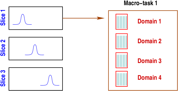
Fig. 5: The two main levels of parallelism in EVSL.

3 The EVSL package

EVSL is a package that provides a collection of spectrum slicing algorithms and projection methods for solving eigenvalue problems. In this section, we address the software design and features of EVSL, its basic functionalities, and its user interfaces.

3.1 Software design and user interface

EVSL is written in C with an added Fortran interface and it is designed primarily for large and sparse eigenvalue problems in both the standard and the generalized forms, where the sparse matrices are stored in the CSR format. The main functions of EVSL are listed next. Two algorithms for computing spectral densities, namely, the kernel polynomial method kpmdos and the Lanczos algorithm landos, and the corresponding spectrum slicers, spslicer and spslicer2 are included in EVSL. Two filter options are available in EVSL, one based on Chebyshev polynomial expansions and the other one based on least-squares (L-S) rational approximations. These are built by the functions find_pol and find_ratf respectively. EVSL also includes 5 projection methods for eigenvalue problems:

• Polynomial filtered non-restart Lanczos algorithm ChebLanNr,

• Rational filtered non-restart Lanczos algorithm RatLanNr,

• Polynomial filtered thick-restart Lanczos algorithm ChebLanTr,

• Rational filtered thick-restart Lanczos algorithm RatLanTr, and

• Polynomial filtered subspace iterations ChebSI.

Two auxiliary functions named LanBounds and LanTrbounds implement simple Lanczos iterations and a more reliable thick-restart version to provide sufficiently good estimations of the smallest and the largest eigenvalues, which are needed to transform the spectrum onto $[-1,1]$ by the polynomial filtering approach. A subroutine named lsPol computes Chebyshev polynomial expansions that approximate functions $f(t)=t^{-1}$ and $f(t)=t^{-1/2}$ in a least-squares sense. This is used to approximate the operations $B^{-1}v$ and $B^{-1/2}v$ as required by the DOS algorithms and the polynomial filtering algorithm for generalized problems. The accuracy of this approximation relies on the condition number of $B$ [57]. For many applications from finite element discretization, the matrix $B$ is the mass matrix, which is often very well-conditioned after a proper diagonal scaling. To solve linear systems with $A-\sigma_{j}B$, EVSL currently relies on sparse direct methods. Along with the library that contains the above mentioned algorithms, test programs are also provided to demonstrate the use of EVSL with finite difference Laplacians on regular grids and general matrices stored under the MatrixMarket format.

The algorithms in EVSL can also be used in a ‘matrix-free’ form that relies on user-defined matrix-vector multiplication functions and functions for solving the involved linear systems. These functions have the following generic prototypes to allow common interfaces with user-specific functions:

typedef void (*NAME)(double *x, double *y, void *data)

and

typedef void (*NAME)(double *x_Re, double *x_Im, double *y_Re, double *y_Im, void *data)

for the computations in real and complex arithmetics, where vector x is the input, vector y is the output and data points to all the required data to perform the function. Below are two sample code snippets to illustrate the common user interfaces of EVSL. The first example shows a call to lanDos to slice the spectrum followed by calls to the polynomial filtering with ChebLanNr to compute the eigenvalues of $(A,B)$ contained in an interval $(\xi,\eta)$ with CSR matrices Acsr and Bcsr. A sparse direct solver is first setup for the solve with $B$ and $L^{\mathsf{T}}$ where $B=LL^{\mathsf{T}}$ (lines 9-11). Then, a lower and an upper bounds of the spectrum are obtained by LanTrbounds (line 11). The DOS is computed by lanDos followed by the spectrum slicing with spslicer2. Finally, we construct a polynomial filter for each slice using find_pol and combine the filter with ChebLanNr to extract the eigenvalues contained in the slice (lines 15-19).

⬇

1/* Example 1: ChebLanNr for (A,B) */

2#include "evsl.h"

3EVSLStart();

4SetGenEig();

5SetAMatrix(&Acsr);

6SetBMatrix(&Bcsr);

7SetupBSolDirect(&Bcsr, &Bsol);

8SetBSol(BSolDirect, Bsol);

9SetLTSol(LTSolDirect, Bsol);

10LanTrbounds(..., &lmin, &lmax);

11intv[0] = xi; intv[1] = eta; intv[2] = lmin; intv[3] = lmax;

12lanDos(..., npts, xdos, ydos, &nev_est, intv);

13spslicer2(xdos, ydos, nslices, npts, sli);

14for (i = 0; i < nslices; i++) {

15 intv[0] = sli[i]; intv[1] = sli[i+1];

16 find_pol(intv, &pol);

17 ChebLanNr(intv, ..., &pol, &nev, &lam, &Y, &res, ...);

18}

19EVSLFinish();

The second example shows a code that uses rational filtering with a call to RatLanNr. The rational filter is built by find_ratf. For each pole of the rational filter, we setup a direct solver for the corresponding shifted matrix and save the data for all the solvers in rat. Once the rational filter is properly setup, RatLanNr can be invoked with it.

⬇

1/* Example 2: RatLanNr for (A,B) */

2for (i = 0; i < nslices; i++) {

3 intv[0] = sli[i]; intv[1] = sli[i+1];

4 intv[2] = lmin; intv[3] = lmax;

5 find_ratf(intv, &rat);

6 void **sol = (void **)malloc(num_pole * sizeof(void *));

7 SetupASIGMABSolDirect(&Acsr, &Bcsr, num_pole, rat, sol);

8 SetASigmaBSol(&rat, ASIGMABSolDirect, sol);

9 RatLanNr(intv, ..., &rat, &nev, &lam, &Y, &res, ...);

10}

3.2 Availability and dependencies

EVSL is available from its website http://www.users.cs.umn.edu/~saad/software/EVSL/index.html and also from the development website https://github.com/eigs/EVSL. EVSL requires the dense linear algebra package BLAS [34, 15, 14] and LAPACK [1]. Optimized high performance BLAS and LAPACK routines, such as those from Intel Math Kernel Library (MKL) and OpenBLAS [52], and sparse matrix-vector multiplication routines are suggested for obtaining good performance. For the linear system solves, CXsparse [11] is distributed along with EVSL as the default sparse direct solver. However, it is possible, and we highly recommended to configure EVSL with other external high performance direct solvers, such as Cholmod [9] and UMFpack [12] from SuiteSparse, and Pardiso [45] with the unified interface prototype. Wrappers with this interface can be easily written for other solver options.

4 Numerical experiments

In this section, we provide a few examples to illustrate the performance and ability of EVSL. In the tests we compute interior eigenvalues of Laplacian matrices and Hamiltonian matrices from electronic structure, and we also solve generalized eigenvalue problems from a Maxwell electromagnetics problems. The experiments were carried out on one node of Catalyst, a cluster at Lawrence Livermore National Laboratory, which is equipped with a dual-socket Intel Xeon E5-2695 processor (24 cores) and 125 GB memory. The EVSL package was compiled with the Intel icc compiler and linked with the threaded Intel MKL for the BLAS/LAPACK and the sparse matrix-vector multiplication routines.

4.1 Laplacian matrices

We begin with discretized Laplacians obtained from the 5-point and 7-point finite-difference schemes on regular 2-D and 3-D grids. In each column of Table 2, we list the grid sizes for each test case, the size of the matrix ($n$), the number of the nonzeros ($nnz$), the spectral interval ($[a,b]$), two intervals of interest from which to extract eigenvalues ($[\xi,\eta]$), and the actual numbers of the eigenvalues contained in $[\xi,\eta]$, denoted by $\nu_{[\xi,\eta]}$.

Table 2: Discretized 5-pt/7-pt Laplacians on 2-D/3-D regular grids.

Grid	n	nnz	$[a,b]$	$[\xi,\eta]$	$\nu_{[\xi,\eta]}$
$343^{2}$	$117,649$	$586,873$	$[0,7.9998]$	$[0.40,0.436]$	356
				$[1.00,1.033]$	347
$729^{2}$	$531,441$	$2,654,289$	$[0,7.9998]$	$[0.40,0.410]$	446
				$[1.00,1.009]$	435
$1000^{2}$	$1,000,000$	$4,996,000$	$[0,7.9998]$	$[0.40,0.405]$	429
				$[1.00,1.005]$	460
$49^{3}$	$117,649$	$809,137$	$[0,11.9882]$	$[0.40,0.570]$	343
				$[1.00,1.100]$	345
$81^{3}$	$531,441$	$3,680,721$	$[0,11.9882]$	$[0.40,0.450]$	433
				$[1.00,1.028]$	420
$100^{3}$	$1,000,000$	$6,940,000$	$[0,11.9882]$	$[0.40,0.428]$	454
				$[1.00,1.018]$	475

Table 3 shows test results for computing the eigenvalues of the Laplacians in the given intervals and the corresponding eigenvectors using ChebLanNr, where ‘deg’ is the degree of the polynomial filter, ‘iter’ indicates the number of Lanczos iterations and ‘nmv’ stands for the number of matrix-vector products required. For the timings, we report the time for computing the matrix-vector products (‘t-mv’), the time for performing the reorthogonalization (‘t-orth’), and the total time to solution (‘t-tot’). As shown, the interval that is deeper inside the spectrum requires a higher-degree polynomial filter and more iterations as well to extract all the eigenvalues, in general. This makes the computation more expensive than with the other interval for computing roughly the same number of eigenvalues. This issue was known from the results in [36]. For the two largest 2-D and 3-D problems, the total time was dominated by the time of performing the matrix-vector products.

Table 3: Polynomial filtered Lanczos algorithm for discretized Laplacians. Times are measured in seconds.

Grid	$[\xi,\eta]$	deg	niter	nmv	iter
					t-mv	t-orth	t-tot
$343^{2}$	$[0.40,0.4360]$	157	1,290	203,200	10.66	24.11	51.95
	$[1.00,1.0330]$	256	1,310	336,219	17.39	25.48	66.71
$729^{2}$	$[0.40,0.4100]$	557	1,610	898,330	182.51	168.20	497.78
	$[1.00,1.0090]$	936	1,590	1,490,547	294.33	179.45	679.08
$1000^{2}$	$[0.40,0.4050]$	1,111	1,530	1,702,481	1451.40	308.98	2410.99
	$[1.00,1.0050]$	1,684	1,670	2,816,108	2402.99	367.49	3804.91
$49^{3}$	$[0.40,0.5700]$	43	1,290	55,899	3.81	26.53	41.03
	$[1.00,1.1000]$	107	1,270	136,449	9.80	24.25	47.00
$81^{3}$	$[0.40,0.4500]$	141	1,590	224,905	77.24	189.91	359.61
	$[1.00,1.0280]$	378	1,570	594,636	191.42	168.33	494.66
$100^{3}$	$[0.40,0.4280]$	248	1,710	425,030	563.36	398.70	1250.26
	$[1.00,1.0180]$	588	1,830	1,077,689	1357.12	426.17	2314.43

Table 4 presents test results when using RatLanNr to solve the same problems given in Table 2. We used the sparse direct solver Pardiso from the Intel MKL to solve the complex symmetric linear systems when applying the rational filter. Comparing the CPU times (t-tot) in this table with those in Table 3, we can see that it is more efficient to use the rational filtered Lanczos algorithm for the 2-D problems than the polynomial filtered counterpart. The numbers in the columns labeled ‘fact-fill’ and ‘fact-time’ are the fill-factors (defined as the ratio of the number of nonzeros of the factors over the number of nonzeros of the original matrix) and the CPU times for factoring the shifted matrices, respectively. For the 2-D problems, the fill-factors stay low and the factorizations are inexpensive. On the other hand, for the 3-D problems, the sparse direct solver becomes much more expensive: it is not only that the factorizations become much more costly, as reflected by the higher and rapidly increasing fill-factors, but that the solve phase of the direct solver, performed at each iteration, becomes more time consuming as well. The timings for performing the solves are shown in the column labeled ‘t-sv’. Consequently, for the 3-D problems the rational filtered Lanczos algorithm is less efficient than the polynomial filtered algorithm. Finally, it is worth mentioning that the rational filtered Lanczos algorithm required far fewer iterations than the polynomial filtered algorithm (about half). This indicates that the quality of the rational filter is better than the polynomial filter with the default threshold. Rational filters are much more effective in amplifying the eigenvalues in a target region while damping the unwanted eigenvalues.

Table 4: Rational filtered Lanczos algorithm for discretized Laplacians. Times are measured in seconds.

Grid	$[\xi,\eta]$	niter	nsv	fact		iter
				fill	time	t-sv	t-orth	t-tot
$343^{2}$	$[0.40,0.4360]$	590	1,184	10.3	0.62	39.23	6.11	50.45
	$[1.00,1.0330]$	590	1,184			38.13	5.23	47.66
$729^{2}$	$[0.40,0.4100]$	730	1,464	13.0	2.50	274.70	37.86	339.02
	$[1.00,1.0090]$	710	1,424			269.14	37.38	331.58
$1000^{2}$	$[0.40,0.4050]$	710	1,424	14.1	4.77	534.90	75.46	659.40
	$[1.00,1.0050]$	750	1,504			559.76	86.11	706.61
$49^{3}$	$[0.40,0.5700]$	630	1,264	68.6	1.90	168.56	6.43	180.11
	$[1.00,1.1000]$	610	1,224			159.86	5.97	170.63
$81^{3}$	$[0.40,0.4500]$	750	1,504	149.7	28.77	1850.33	42.14	1923.36
	$[1.00,1.0280]$	730	1,464			1813.15	40.40	1882.21
$100^{3}$	$[0.40,0.4280]$	810	1,624	186.3	87.64	4343.00	104.30	4510.28
	$[1.00,1.0180]$	930	1,864			5035.75	127.28	5240.53

4.2 Spectral slicing

In this set of experiments, we show performance results of the spectrum slicing algorithm with KPM in EVSL, where we computed all the $1,971$ eigenvalues in the interval $[0,1]$ of the 7-point Laplacian matrix on the 3-D grid of size $49\times 49\times 49$. The interval $[0,1]$ was first partitioned into up to $6$ slices in such a way that each slice contains roughly the same number of eigenvalues. Then, ChebLanNr was used to extract the eigenvalues in each slice individually. The column labeled $\nu_{[\xi,\eta]}$ in Table 5 lists the number of eigenvalues contained in the divided subintervals, which are fairly close to each other across the slices. For the iteration time ‘t-tol’, since on parallel machines, a parallelized EVSL code can compute the eigenvalues in different slices independently, the total time of computing all the eigenvalues in the whole interval will be the maximum iteration time across all the slices. As shown, compared with the CPU time required by the solver with a single slice, significant CPU time reduction can be achieved with multiple slices.

With regard to load balancing, the memory requirements were very well balanced across the slices, since the memory allocation in the Lanczos algorithm is proportional to the number of eigenvalues to compute. Note also that the iteration times shown in the column labeled ‘t-tol’ were also reasonably well balanced, except for the first slice which is a “boundary slice” on the left end of the spectrum. A special type of polynomial filters were used for boundary slices, which usually have lower degrees than with the filters for the internal slices. Moreover, the convergence rates for computing the eigenvalues for boundary slices are typically better, as reflected by the smaller number of iterations. Therefore, the total iteration time for the first slice is much smaller than with the other slices. Starting with the second slice, the overall iteration time did not change dramatically. This is in spite of the fact that the required degree of the polynomial filter keeps increasing as the slice moves deeper inside the spectrum leading to a higher cost for applying the filters each time. The explanation is that in these problems the cost of performing matrix-vector products was insignificant relative to the cost of the reorthogonalizations.

Table 5: Polynomial filtered Lanczos algorithm for computing $1,971$ eigenvalues of a Laplacian of size $49^{3}$ within $[0,1]$.

Slices	$[\xi,\eta]$	$\nu_{[\xi,\eta]}$	deg	niter	nmv	iter
						t-mv	t-orth	t-tot
1	$[0.00000,1.00000]$	1,971	5	4,110	22,531	2.07	224.97	353.09
2	$[0.00000,0.65863]$	997	6	2,230	14,389	1.34	69.92	107.76
	$[0.65863,1.00000]$	974	28	3,470	98,190	7.06	173.09	240.64
3	$[0.00000,0.51208]$	657	7	1,510	11,241	1.06	34.43	52.09
	$[0.51208,0.78294]$	662	31	2,390	74,814	5.66	88.42	126.46
	$[0.78294,1.00000]$	652	46	2,350	108,844	7.79	76.49	116.00
4	$[0.00000,0.42983]$	495	8	1,150	9,711	0.92	20.10	30.23
	$[0.42983,0.65394]$	484	35	1,770	62,504	4.71	44.65	68.66
	$[0.65394,0.83844]$	502	49	1,850	91,250	6.07	45.80	70.80
	$[0.83844,1.00000]$	490	62	1,850	115,314	7.65	48.38	76.45
5	$[0.00000,0.37793]$	386	8	970	8,162	0.73	15.34	22.46
	$[0.37793,0.57373]$	401	37	1,450	54,125	4.00	29.74	46.00
	$[0.57373,0.73473]$	399	53	1,470	78,415	5.73	29.43	48.69
	$[0.73473,0.87424]$	400	68	1,450	99,136	7.36	29.89	51.41
	$[0.87424,1.00000]$	385	81	1,430	116,377	8.83	29.51	53.57
6	$[0.00000,0.33926]$	329	9	810	7,637	0.68	13.30	20.84
	$[0.33926,0.51429]$	328	40	1,212	48,808	3.68	23.85	37.20
	$[0.51429,0.65913]$	340	56	1,230	69,332	4.96	25.57	41.03
	$[0.65913,0.78384]$	322	72	1,230	89,026	6.29	25.65	44.98
	$[0.78384,0.89719]$	345	85	1,230	105,065	7.42	26.21	46.52
	$[0.89719,1.00000]$	307	100	1,190	119,507	8.13	23.93	43.53

4.3 Hamiltonian matrices

In this set of experiments, we computed eigenpairs of 5 Hamiltonian matrices from the Kohn-Sham equations for density functional theory calculations. These matrices are available from the PARSEC group in the SuiteSparse Matrix Collection [13]. The matrix size $n$, the number of the nonzeros $nnz$ and the range of the spectrum $[a,b]$ are provided in Table 6. Each Hamiltonian has a number of occupied states of the chemical compound and this number is often denoted by $n_{0}$. In Density Functional Theory (DFT), the $n_{0}$-th smallest eigenvalue corresponds to the Fermi level. As in [20], we computed all the eigenvalues contained in the interval $[0.5n_{0},1.5n_{0}]$ and the corresponding eigenvectors. The target intervals, which are denoted by $[\xi,\ \eta]$, and the numbers of the eigenvalues inside the intervals are given in the last two columns of Table 6.

Table 6: Hamiltonian matrices from the PARSEC set

Matrix	n	nnz	$[a,b]$	$[\xi,\eta]$	$\nu_{[\xi,\eta]}$
$\mathrm{Ge_{87}H_{76}}$	$112,985$	$7,892,195$	$[-1.214,32.764]$	$[-0.645,-0.0053]$	212
$\mathrm{Ge_{99}H_{100}}$	$112,985$	$8,451,295$	$[-1.226,32.703]$	$[-0.650,-0.0096]$	250
$\mathrm{Si_{41}Ge_{41}H_{72}}$	$185,639$	$15,011,265$	$[-1.121,49.818]$	$[-0.640,-0.0028]$	218
$\mathrm{Si_{87}H_{76}}$	$240,369$	$10,661,631$	$[-1.196,43.074]$	$[-0.660,-0.0300]$	213
$\mathrm{Ga_{41}As_{41}H_{72}}$	$268,096$	$18,488,476$	$[-1.250,1300.9]$	$[-0.640,-0.0000]$	201

We first report in Table 7 the performance results of ChebLanNr for computing the eigenvalues of the Hamiltonians in the target interval. For the first 4 matrices, the polynomial degrees used in the filters are relatively low so that the cost of the matrix-vector products is not high relative to the cost of the reorthogonalizations. Extracting eigenvalues from the last matrix was more challenging because its spectrum is much wider than the others, with the result that a polynomial filter of a much higher degree was needed resulting in a much higher cost for matrix-vector products. Similar results were also reported in [20].

Table 7: Numerical results of polynomial filtered Lanczos algorithm for PARSEC matrices.

Matrix	deg	niter	nmv	iter
				t-mv	t-orth	t-tot
$\mathrm{Ge_{87}H_{76}}$	26	990	26,004	28.53	14.88	50.05
$\mathrm{Ge_{99}H_{100}}$	26	1,090	28,642	33.71	17.52	59.18
$\mathrm{Si_{41}Ge_{41}H_{72}}$	32	950	30,682	71.61	28.82	112.11
$\mathrm{Si_{87}H_{76}}$	29	1,010	29,561	46.38	30.27	89.92
$\mathrm{Ga_{41}As_{41}H_{72}}$	172	910	157,065	497.39	29.25	558.26

Next, we present the performance results of RatLanNr in Table 8. An issue we confronted when using this algorithm for this set of matrices is that the factorization of the shifted matrix becomes prohibitively expensive, in terms of both the memory requirement as indicated by the high fill-ratios (e.g., the factorization of the last matrix required 42 GB memory), and the high factorization time (remarkably, this is even higher than the total iteration time with the polynomial filter). Despite requiring only about half of the number of iterations that were needed by ChebLanNr, the total iteration time using the rational filter was still much higher, since the solve phase of the direct solver was also much more expensive compared with the matrix-vector products performed in the polynomial filtered Lanczos algorithm.

Table 8: Numerical results of rational filtered Lanczos algorithm for PARSEC matrices.

Matrix	niter	nsv	fact		iter
			fill	time	t-sv	t-orth	t-tot
$\mathrm{Ge_{87}H_{76}}$	450	904	149.2	120.56	2022.33	4.03	2029.11
$\mathrm{Ge_{99}H_{100}}$	490	984	146.5	152.07	2259.01	4.01	2266.42
$\mathrm{Si_{41}Ge_{41}H_{72}}$	430	864	178.9	447.89	4587.51	7.09	4599.10
$\mathrm{Si_{87}H_{76}}$	450	904	376.9	718.00	7058.93	9.71	7074.30
$\mathrm{Ga_{41}As_{41}H_{72}}$	410	824	378.5	865.43	7456.54	9.97	7472.38

4.4 Generalized eigenvalue problems: the Maxwell Eigenproblem

We consider the Maxwell electromagnetic eigenvalue problem with homogeneous Dirichlet boundary conditions:

$$\nabla\times\nabla\times\vec{E} =\lambda\vec{E},\quad\lambda=\omega^{2}/c^{2},\quad\mbox{in}\quad\Omega,$$

$$\nabla\cdot\vec{E} =0,\quad\mbox{in}\quad\Omega,$$

$$\vec{E}\times\vec{n} =0,\quad\mbox{on}\quad\partial\Omega,$$ (26)

where $\vec{E}$ is the electric field, $\vec{n}$ is the unit outward normal to the boundary $\partial\Omega$, $\omega$ is the eigenfrequency of the electromagnetic oscillations, and $c$ is the light velocity. The curl-curl operator was discretized using a Nédélec finite element space of the second order in 2D or 3D. Our goal is to find the electromagnetic eigenmodes that are the non-zero solutions of (4.4). As shown in [3], the discretized problem (4.4) is equivalent to the matrix eigenvalue problem $Ax=\lambda Bx$, where $A$ is the stiffness matrix corresponding to the curl-curl operator and $B$ is the mass matrix. It is well-known that the matrix $A$ has a high-dimensional zero eigenspace spanned by discretized gradients. Therefore, the desired positive eigenvalues are deep inside the spectrum. In Figure 6, we show the spectrum of $B^{-1}A$ for a 2-D problem on a square disc and the spectrum for a 3-D problem on a cube. The 2-D problem is of size $3600$ (after eliminating the degrees of freedom on the boundary), where about $32\%$ of the eigenvalues ($1137$ out of $3600$) are clustered around zero and the smallest eigenvalue that is away from zero is $6.71$. The 3-D problem is of size $10800$ which also has about $32\%$ of the eigenvalues ($3375$ out of $10800$) close to zero and the smallest eigenvalue that is away from zero is $19.80$. A few of the non-zero eigenmodes of both problems are illustrated in Figure 7.

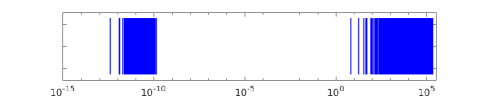
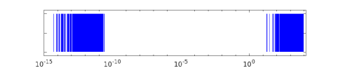
Fig. 6: Spectrum of the Maxwell eigenproblem on a 2-D square-disc and on a 3-D cube

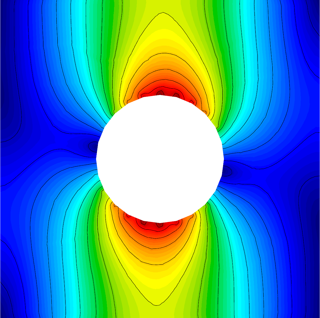
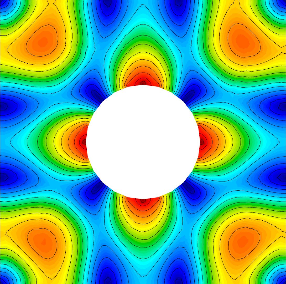
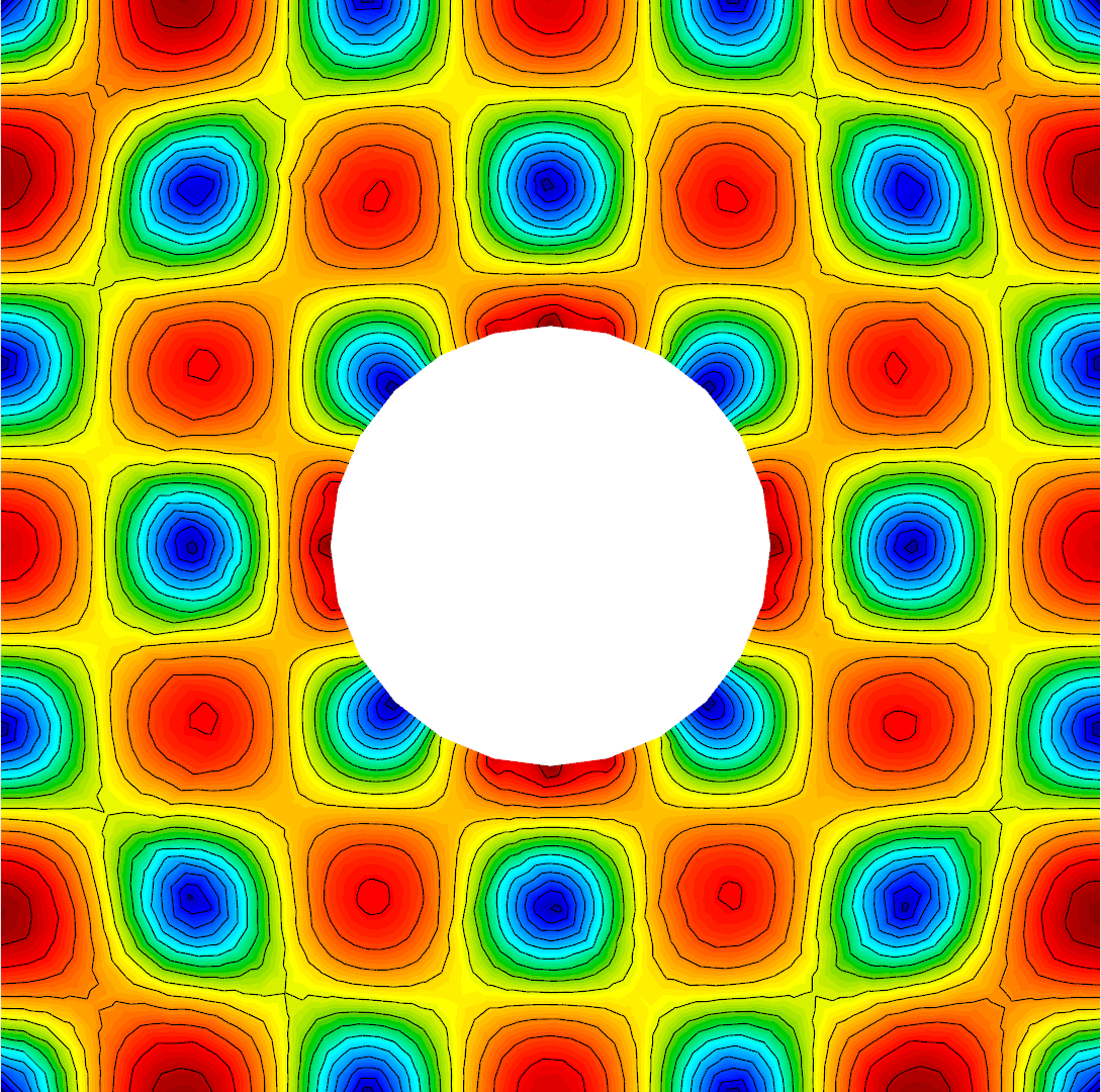
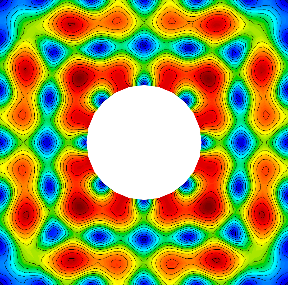
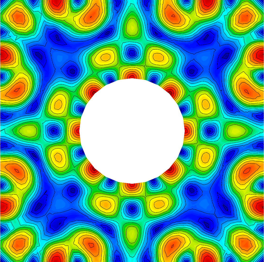
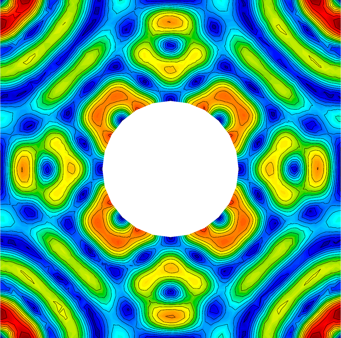
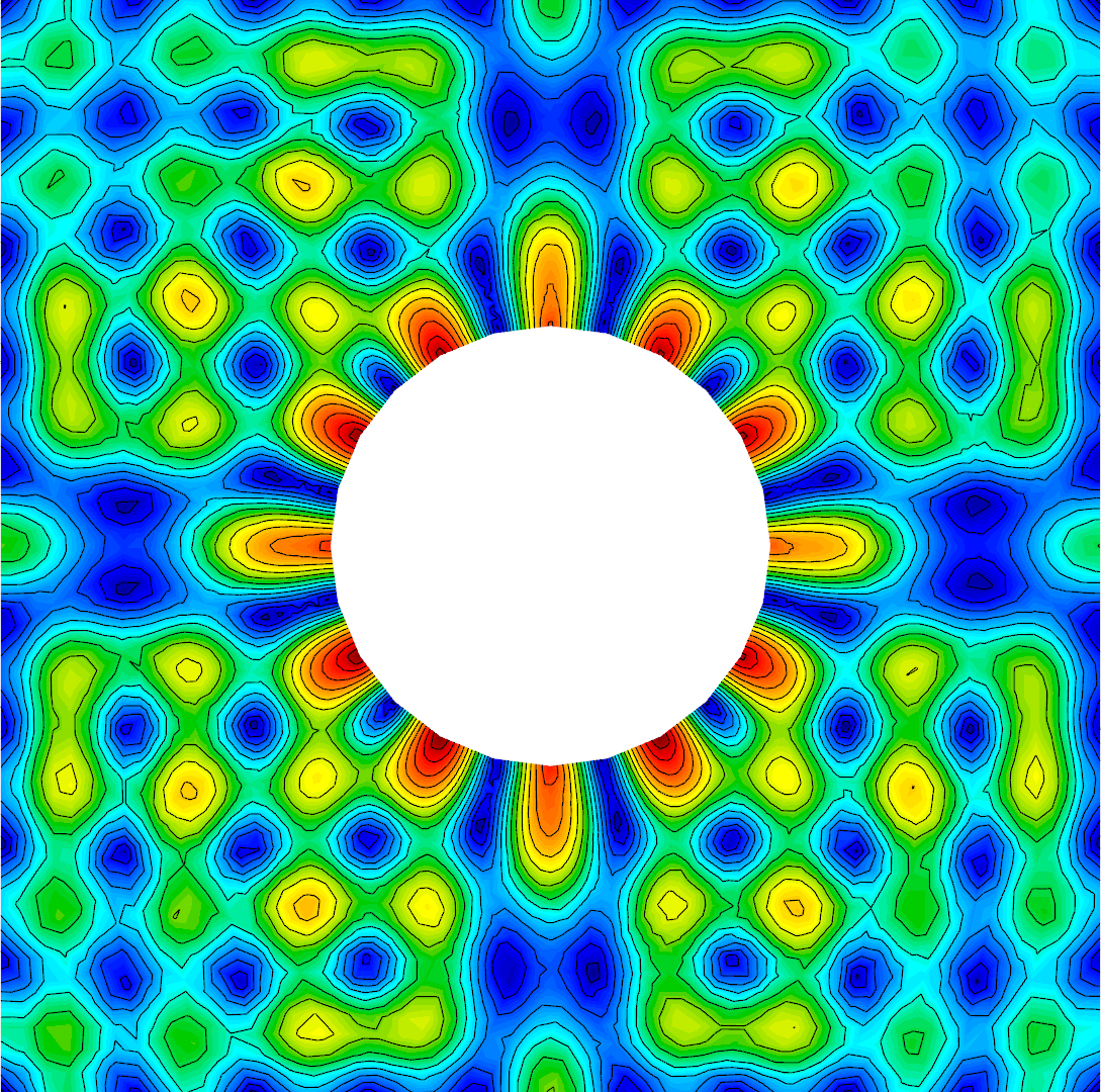
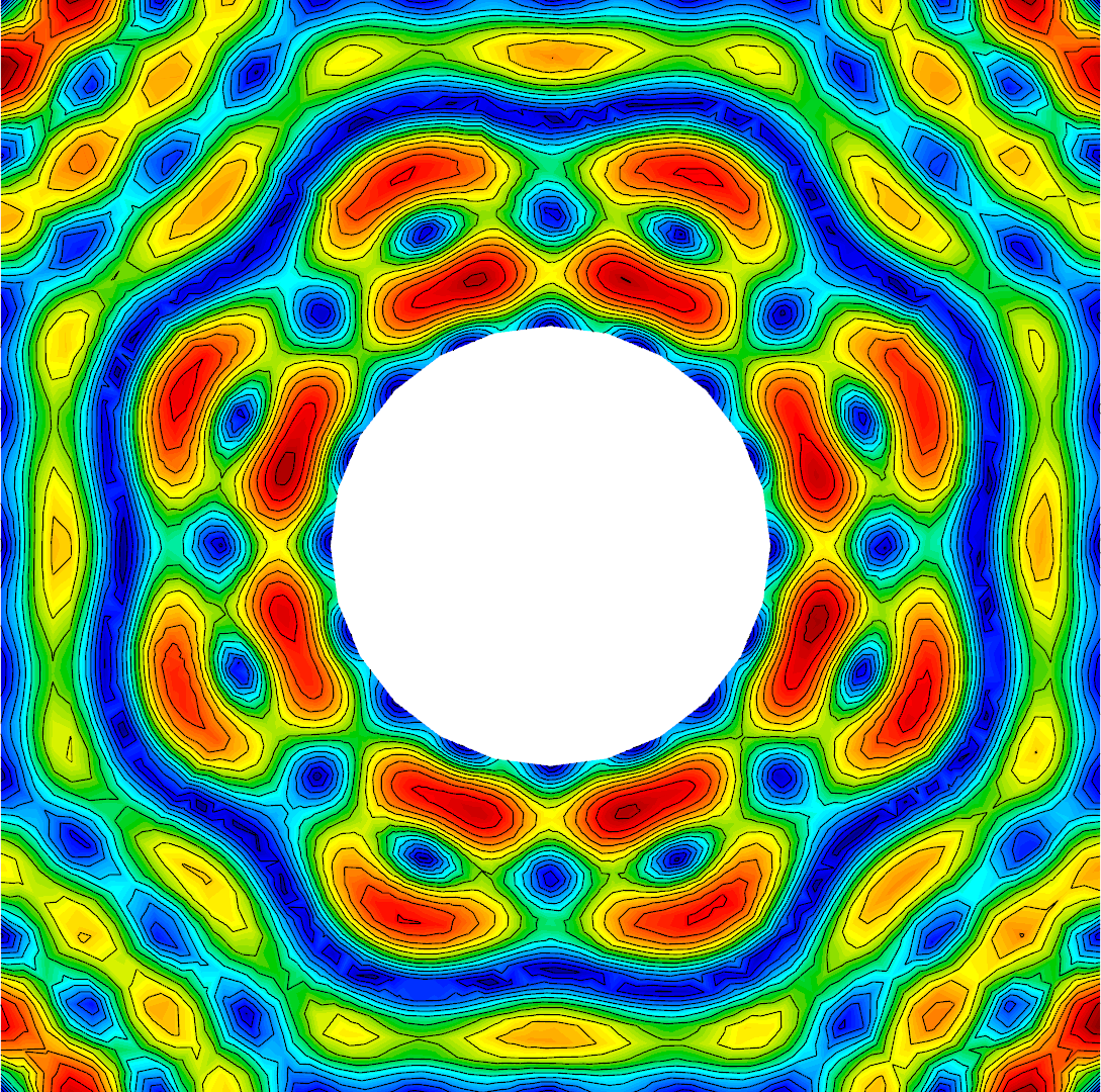
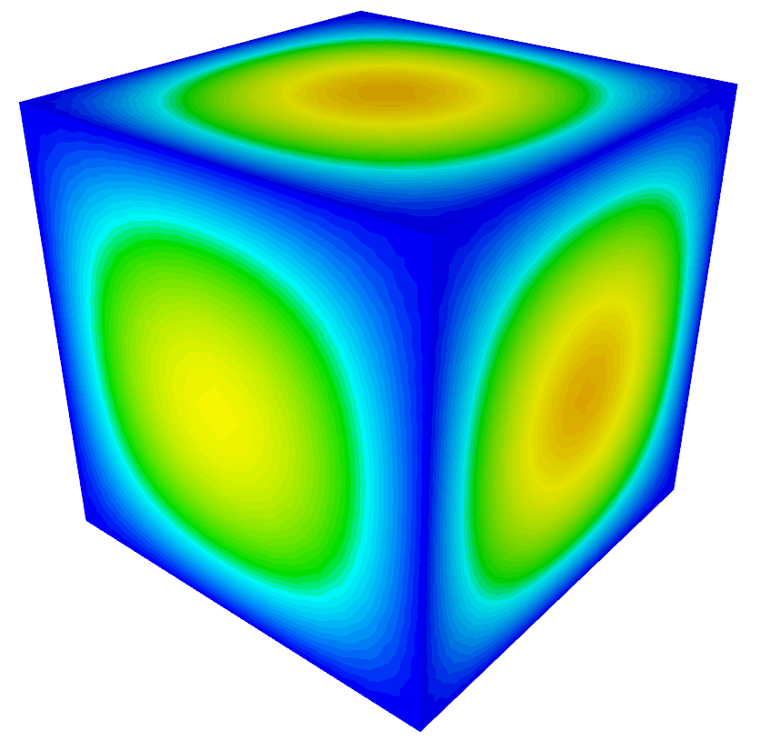
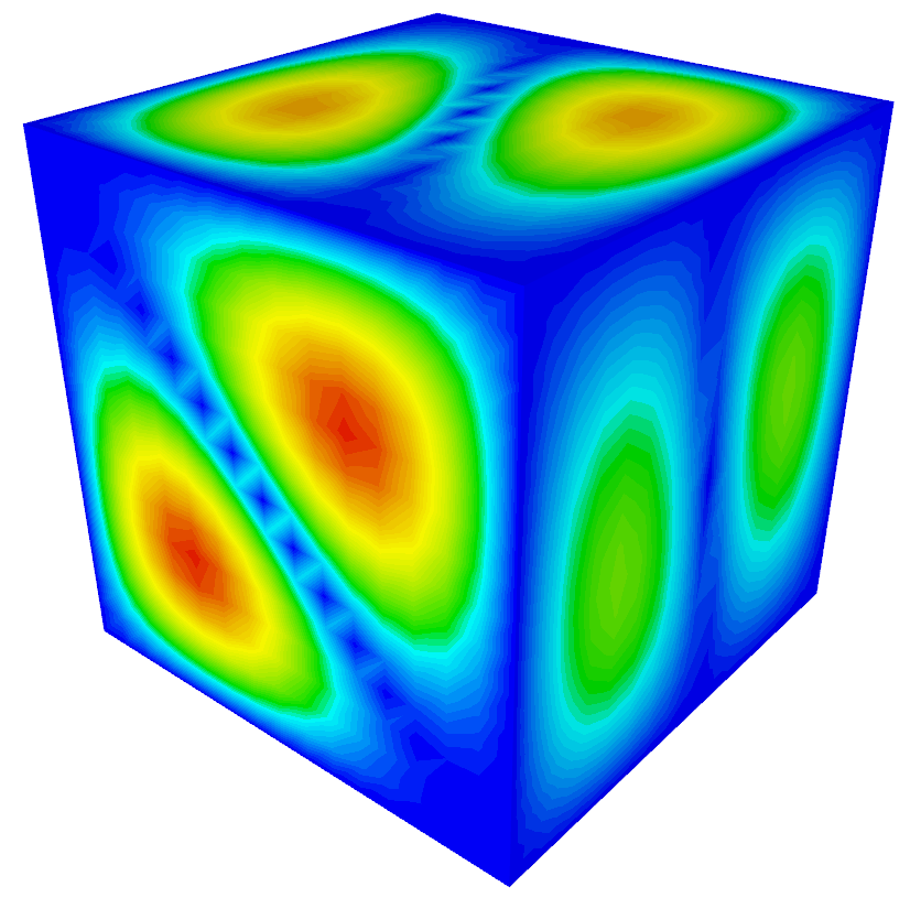
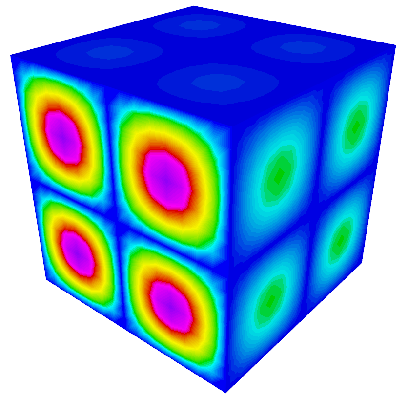
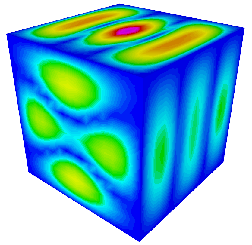
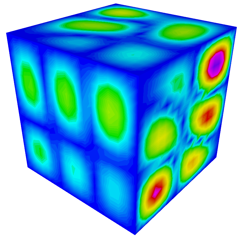
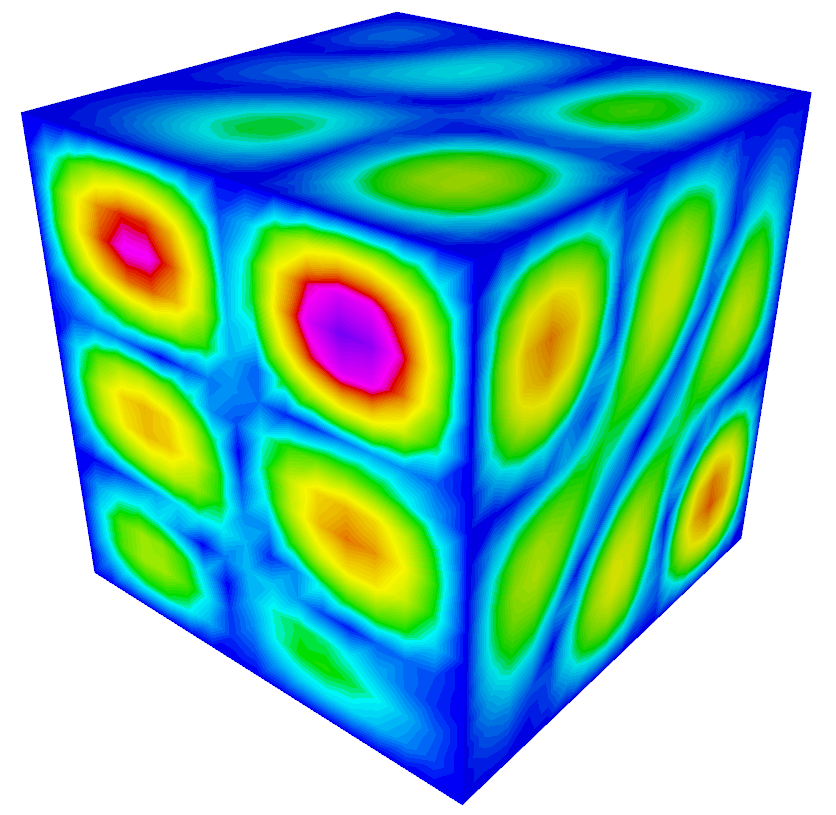
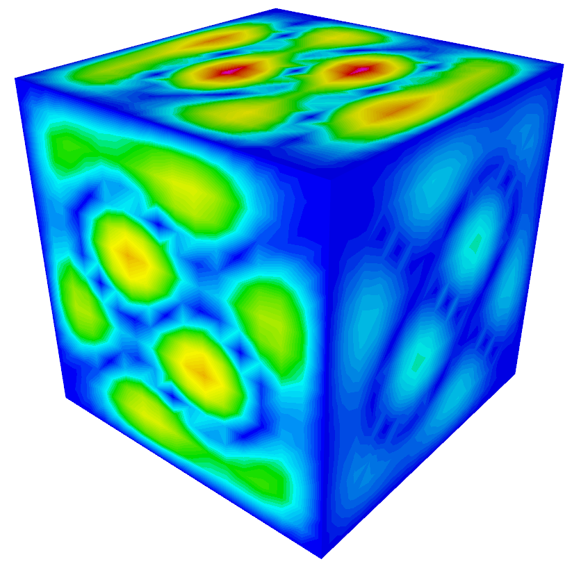
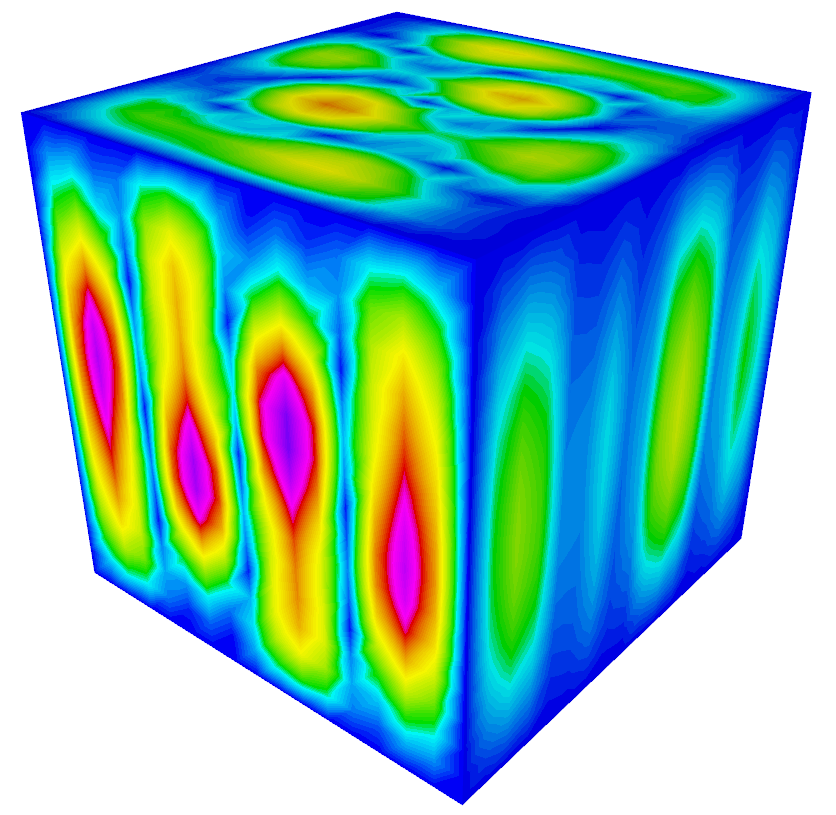
Fig. 7: An illustration of the 1st, 10th, 18th, 29th, 49th, 59th, 65th and 75th electromagnetic eigenmodes of the Maxwell eigenproblem on a 2-D square-disc and on a 3-D cube

In cases where the knowledge of the kernel space of $A$ is known from the discretization, say $\mbox{Ker}(A)=\mbox{span}\left\{y_{1},\ldots,y_{m}\right\}$, this information can be used to design more efficient specialized Maxwell eigensolvers. For instance, in the Auxiliary Maxwell Eigensolver (AME) [50], the $B$-orthogonal projector

$$P=I-Y(Y^{\mathsf{T}}BY)^{-1}Y^{\mathsf{T}}B,$$ (27)

where $Y=[y_{1},\ldots,y_{m}]$, is applied within LOBPCG to force the iterations to remain in the subspace $\mbox{Ran}(Y)^{\perp_{B}}$. The same projection was also exploited in [3] as the preconditioner of the implicitly restarted Lanczos algorithm and the Jacobi-Davidson algorithm. However, we remark here that these solvers are not purely algebraic solvers since additional information from the discretization is assumed. On the other hand, with EVSL’s filtering mechanism, it is straightforward to skip the zero eigenvalues and jump to the desired part of the spectrum. In Table 9, we list the 8 Maxwell eigenvalue problems considered, for which we computed all the eigenvalues in the given interval ${[\xi,\eta]}$ and the corresponding eigenvectors.

Table 9: Maxwell eigenvalue problems

Problem	n	nnz	$(a,b)$	$(\xi,\eta)$	$\nu_{[\xi,\eta]}$
Max2D-1	14,592	72,200	$(0,9.64\times 10^{5})$	$(6,1200)$	$96$
Max2D-2	59,520	292,216	$(0,4.00\times 10^{6})$	$(6,1200)$	$96$
Max2D-3	235,776	1,175,816	$(0,1.62\times 10^{7})$	$(6,1200)$	$96$
Max2D-4	944,640	4,717,064	$(0,6.50\times 10^{7})$	$(6,1200)$	$96$
Max3D-1	10,800	320,952	$(0,8.96\times 10^{3})$	$(19.5,250)$	$115$
Max3D-2	92,256	2,893,800	$(0,3.66\times 10^{4})$	$(19.5,250)$	$121$
Max3D-3	762,048	24,526,920	$(0,1.47\times 10^{5})$	$(19.5,250)$	$121$
Max3D-4	2,599,200	84,363,432	$(0,3.32\times 10^{5})$	$(19.5,250)$	$121$

We first present the results with ChebLanNr in Table 10. For the solves with $B$, which is a very well-conditioned mass matrix, we considered using the sparse direct solver Pardiso and the Chebyshev polynomial expansion by lsPol. These two methods are indicated as ‘d’ and ‘c’ in the column labeled ‘sv’ of Table 10 respectively. For each problem we present the result with the method for the solves with $B$ that yielded the better total iteration time. We found that for larger problems, in both 2-D and 3-D, using the Chebyshev iterations yielded better iteration times, while for the 3 smaller problems using the direct solver was more efficient. In the column ‘niter’, we give the numbers of the iterations required by the filtered Lanczos algorithm, which remained roughly the same as the problem sizes increase and thus, so did the convergence rates. In order to keep such constant convergence rates, the required degree of the polynomial filter (shown in column ‘deg’) needed to increase, since the target interval $[\xi,\eta]$ was unchanged but the spectrum of $B^{-1}A$ becomes wider as the problem size increases. For the iteration time, the cost of performing the solves with $B$ (t-sv) dominated the total iteration time (t-tot), which is much more expensive than the cost of computing the matrix-vector products with $A$ (t-mv) and the cost of the orthogonalization (t-orth).

Table 10: Numerical results of the polynomial filtered Lanczos algorithm for Maxwell eigenvalue problems

Problem	deg	niter	sv	fact		iter
				mem	time	t-mv	t-sv	t-orth	t-tot
Max2D-1	69	350	d	5 MB	0.19	0.90	31.7	0.32	35.24
Max2D-2	141	350	d	21 MB	0.24	2.75	221.0	1.89	233.63
Max2D-3	284	350	c	-	-	22.89	616.50	7.07	946.62
Max2D-4	570	350	c	-	-	279.20	10238.2	45.39	10585.81
Max3D-1	15	530	d	32 MB	0.24	0.34	9.62	0.71	11.42
Max3D-2	30	570	c	-	-	6.60	185.16	8.08	203.33
Max3D-3	61	590	c	-	-	137.67	4907.82	78.73	5149.92
Max3D-4	93	570	c	-	-	774.50	27407.41	529.49	28822.21

Next, we examine the performance of RatLanNr shown in Table 11. Pardiso was used to solve the linear systems with $A-\sigma_{j}B$ required by the rational filter. Compared with ChebLanNr, fewer iterations were required and the total iteration time was also much shorter. For the largest 2-D problem, the iteration time required by RatLanNr was $90$ times faster, while for the largest 3-D problem, this speedup was about $3$. In the previous sections, we have seen significant CPU time savings by using ChebLanNr for the 3-D Laplacians and Hamiltonians compared with RatLanNr. However, the results presented in this section indicate the opposite. The reason for the different time efficiency of the two types of methods for standard and generalized eigenvalue problems can be understood from the computations required to apply the filter at each step of the Lanczos iterations that are given in Table 1. Let $k$ denote the degree of the polynomial filter and $k_{j}$ denote the number of the repetition of pole $j$ of the rational filter. In our runs, only one pole, repeated twice, was used, so we have $\sum k_{j}=2$. For standard eigenvalue problems, each step of ChebLanNr requires $k$ matrix-vector products with $A$, whereas each step of RatLanNr needs to perform $\sum k_{j}$ solves with $A-\sigma_{j}B$. For large 3-D problems, it turned out that it was more expensive to perform the solves than the matrix-vector products, so ChebLanNr was usually more efficient. However, for the generalized problems, there are additional $k$ solves with $B$ for each step of ChebLanNr, which makes the application of the polynomial filter significantly much more expensive. In contrast, RatLanNr requires $\sum k_{j}$ matrix-vector products with $B$ additionally, the cost of which is usually negligible. Consequently, RatLanNr was often found to be much more efficient for generalized eigenvalue problems than ChebLanNr.

Table 11: Numerical results of the rational filtered Lanczos algorithm for Maxwell eigenvalue problems

Problem	niter	sv	fact		iter
			mem	time	t-mv	t-sv	t-orth	t-tot
Max2D-1	190	d	9 MB	0.10	.04	.95	0.07	1.15
Max2D-2	190	d	39 MB	0.28	.07	4.36	0.74	5.57
Max2D-3	190	d	168 MB	1.02	0.25	24.34	2.98	29.00
Max2D-4	190	d	716 MB	4.31	1.39	100.55	10.52	117.11
Max3D-1	290	d	95 MB	0.23	0.06	4.95	0.18	5.39
Max3D-2	290	d	923 MB	2.45	0.46	94.65	2.28	98.20
Max3D-3	290	d	13 GB	64.53	5.31	1599.72	20.69	1631.30
Max3D-4	290	d	68 GB	649.21	25.21	9419.12	127.74	9609.42

On the other hand, the memory requirement of RatLanNr is much higher than ChebLanNr, as shown in the columns labeled ‘mem’ of Tables 10-11, due to the large memory consumption of the factorization of $A-\sigma_{j}B$. For the polynomial filtering, we can avoid any factorization by performing the solves with $B$ with iterative methods such as the Chebyshev polynomial iterations. For rational filtering, EVSL currently relies on direct methods to solve the linear systems with the matrices $A-\sigma_{j}B$, which are highly indefinite. This is because it is challenging to find efficient iterative methods to solve linear systems with such matrices.

5 Recommendations, outlook, and closing remarks

Recommendations: Rational vs. polynomial filtering

Based on our experiments, we found that when combined with the Lanczos algorithm, rational filtering tends to be more efficient than polynomial filtering, for 2-D problems in both the standard and generalized forms. This is because the factorization of the shifted matrix $A-\sigma_{j}B$ is generally inexpensive. For large 3-D problems in the standard form, the factorization of $A-\sigma_{j}B$ becomes too expensive and in these cases using the polynomial filtered algorithm tends to be more efficient in terms of both CPU time consumption and memory usage. This can be also true for generalized problems in the situation where linear systems with $B$ are (very) inexpensive to solve. Finally, for the situations where solving linear systems with the $B$ matrix is costly, the rational filtered algorithms may become more efficient in terms of CPU time usage, provided the factorization of $A-\sigma_{j}B$ is still affordable, although it will usually require much more memory. Otherwise, when factoring $A-\sigma_{j}B$ becomes prohibitively expensive, then the alternative of the polynomial filtered algorithm remains a feasible option as long as linear systems with the matrix $B$ can be efficiently solved. There are situations in finite elements discretizations that lead to mass matrices $B$ that are very well conditioned once they are scaled by their diagonals. In these cases, solving a linear system with $B$ and $B^{1/2}$ is quite inexpensive as it can be carried out with a small number of matrix-vector products with $B$, see [57] for details.

Outlook: Parallelism and iterative solvers

A fully parallel version of EVSL using MPI is currently being developed. It is being tested on a large scale geophysics simulation and will be released soon. Obtaining a scalable parallel rational filtered algorithm in a parallel distributed memory environment may be rather challenging because of the limitations of current parallel direct solvers. Polynomial filtered algorithms are more appealing from this perspective since for standard eigenvalue problems, the matrix $A$ is only involved in matrix-vector products, which can be efficiently parallelized. Moreover, as already mentioned, for generalized eigenvalue problems in which the $B$ matrix is well-conditioned, solving systems with $B$ and $B^{1/2}$ can be achieved via the application of low degree polynomials in $B$ to the right-hand side.

We have not yet mentioned the possibility of replacing direct solvers by iterative ones for rational filtering methods, but this is in our future plans. Iterative solvers that will be used in this context must be able to handle highly indefinite systems, and methods derived from those in [59, 56] may be suitable. These methods are highly parallel and must be tuned to the specificity of rational filtering: complex matrices, availability of spectral information, multiple shifts, etc.

Closing remarks

There were attempts more than two decades ago to utilize ideas based on polynomial filtering for solving interior eigenvalue problems but these were abandoned because they were generally found not to be competitive relative to the standard Krylov subspace approaches. Similarly, when the first idea of using Cauchy integrals came about, it was not adopted right away. With the emergence in recent years of very large scale electronic structure calculations, and other scientific simulations, methods that combine filtering and spectrum slicing have become not just appealing, but also mandatory. Their main appeal lies in the extra level of parallelism they offer as well as in their intrinsic efficiency due to the reduced orthogonalization costs that characterize them. Therefore, the reborn versions of spectrum slicing that have recently emerged constitute a new paradigm that is likely to gain in importance.

References

- [1] E. Anderson, Z. Bai, C. Bischof, S. Blackford, J. Demmel, J. Dongarra, J. Du Croz, A. Greenbaum, S. Hammarling, A. McKenney, and D. Sorensen, LAPACK Users’ Guide, Society for Industrial and Applied Mathematics, Philadelphia, PA, third ed., 1999.
- [2] X. Andrade, D. A. Strubbe, U. De Giovannini, A. H. Larsen, M. J. T. Oliveira, J. Alberdi-Rodriguez, A. Varas, I. Theophilou, N. Helbig, M. Verstraete, L. Stella, F. Nogueira, A. Aspuru-Guzik, A. Castro, M. A. L. Marques, and A. Rubio, Real-space grids and the octopus code as tools for the development of new simulation approaches for electronic systems, Physical Chemistry Chemical Physics, 17 (2015), pp. 31371–31396.
- [3] P. Arbenz, R. Geus, and S. Adam, Solving Maxwell eigenvalue problems for accelerating cavities, Physical Review Special Topics-Accelerators and Beams, 4 (2001), p. 022001.
- [4] J. Asakura, T. Sakurai, H. Tadano, T. Ikegami, and K. Kimura, A numerical method for nonlinear eigenvalue problems using contour integrals, JSIAM Letters, 1 (2009), pp. 52–55.
- [5] J. Baglama, D. Calvetti, and L. Reichel, Algorithm 827: Irbleigs: A matlab program for computing a few eigenpairs of a large sparse Hermitian matrix, ACM Trans. Math. Softw., 29 (2003), pp. 337–348.
- [6] C. G. Baker, U. L. Hetmaniuk, R. B. Lehoucq, and H. K. Thornquist, Anasazi software for the numerical solution of large-scale eigenvalue problems, ACM Trans. Math. Softw., 36 (2009), pp. 13:1–13:23.
- [7] M. Bollhöfer and Y. Notay, JADAMILU: a software code for computing selected eigenvalues of large sparse symmetric matrices, Comput. Phys. Commun., 177 (2007), pp. 951 – 964.
- [8] W. R. Burdick, Y. Saad, L. Kronik, Manish Jain, and James Chelikowsky, Parallel implementations of time-dependent density functional theory, Comput. Phys. Comm., 156 (2003), pp. 22–42.
- [9] Y. Chen, T. A. Davis, W. W. Hager, and S. Rajamanickam, Algorithm 887: Cholmod, supernodal sparse cholesky factorization and update/downdate, ACM Trans. Math. Softw., 35 (2008), pp. 22:1–22:14.
- [10] J. W. Daniel, W. B. Gragg, L. Kaufman, and G. W. Stewart, Reorthogonalization and stable algorithms for updating the gram-schmidt qr factorization, Mathematics of Computation, 30 (1976), pp. 772–795.
- [11] T. Davis, Direct Methods for Sparse Linear Systems, Society for Industrial and Applied Mathematics, 2006.
- [12] T. A. Davis, Algorithm 832: Umfpack v4.3—an unsymmetric-pattern multifrontal method, ACM Trans. Math. Softw., 30 (2004), pp. 196–199.
- [13] T. A. Davis and Y. Hu, The university of florida sparse matrix collection, ACM Trans. Math. Softw., 38 (2011), pp. 1:1–1:25.
- [14] J. J. Dongarra, J. Du Croz, S. Hammarling, and I. S. Duff, A set of level 3 basic linear algebra subprograms, ACM Trans. Math. Softw., 16 (1990), pp. 1–17.
- [15] J. J. Dongarra, J. Du Croz, S. Hammarling, and R. J. Hanson, An extended set of fortran basic linear algebra subprograms, ACM Trans. Math. Softw., 14 (1988), pp. 1–17.
- [16] M. Heroux et al., The trilinos project.
- [17] P. Giannozzi et al., Quantum expresso. Available from http://www.quantum-espresso.org.
- [18] T. Sakurai et al., Parallel eigenvalue solvee.
- [19] R. D. Falgout and U. M. Yang, hypre: A library of high performance preconditioners, in Computational Science — ICCS 2002, Peter M. A. Sloot, Alfons G. Hoekstra, C. J. Kenneth Tan, and Jack J. Dongarra, eds., Berlin, Heidelberg, 2002, Springer Berlin Heidelberg, pp. 632–641.
- [20] H. R. Fang and Y. Saad, A filtered Lanczos procedure for extreme and interior eigenvalue problems, SIAM J. Sci. Comput., 34 (2012), pp. A2220–A2246.
- [21] D. R. Fokkema, G. L. G. Sleijpen, and H. A. van der Vorst, Jacobi-Davidson style QR and QZ algorithms for the reduction of matrix pencils, SIAM J. Sci. Comput., 20 (1998), pp. 94–125.
- [22] L. Giraud, J. Langou, M. Rozložník, and J. Van Den Eshof, Rounding error analysis of the classical Gram-Schmidt orthogonalization process, Numer. Math., 101 (2005), pp. 87–100.
- [23] L. Giraud, J. Langou, and M. Rozloznik, The loss of orthogonality in the Gram-Schmidt orthogonalization process, Comput. Math. Appl., 50 (2005), pp. 1069 – 1075.
- [24] X. Gonze, J.-M. Beuken, R. Caracas, F. Detraux, M. Fuchs, G.-M. Rignanese, L. Sindic, M. Verstraete, G. Zerah, F. Jollet, M. Torrent, A. Roy, M. Mikami, Ph. Ghosez, J.-Y. Raty, and D.C. Allan, First-principles computation of material properties: The ABINIT software project, Computational Materials Science, 25 (2002), pp. 478–492.
- [25] Y. Hasegawa, J. Iwata, M. Tsuji, D. Takahashi, A. Oshiyama, K. Minami, T. Boku, F. Shoji, A. Uno, M. Kurokawa, H. Inoue, I. Miyoshi, and M. Yokokawa, First-principles calculations of electron states of a silicon nanowire with 100,000 atoms on the k computer, in Proceedings of 2011 International Conference for High Performance Computing, Networking, Storage and Analysis, SC ’11, New York, NY, USA, 2011, ACM, pp. 1:1–1:11.
- [26] V. Hernández, J. E. Román, and V. Vidal, SLEPc: A scalable and flexible toolkit for the solution of eigenvalue problems, ACM Trans. Math. Softw., 31 (2005), pp. 351–362.
- [27] A. Klinvex, F. Saied, and A. Sameh, Parallel implementations of the trace minimization scheme tracemin for the sparse symmetric eigenvalue problem, Computers and Mathematics with Applications, 65 (2013), pp. 460 – 468. Efficient Numerical Methods for Scientific Applications.
- [28] A. Knyazev, M. Argentati, I. Lashuk, and E. Ovtchinnikov, Block Locally Optimal Preconditioned Eigenvalue Xolvers (BLOPEX) in Hypre and PETSc, SIAM Journal on Scientific Computing, 29 (2007), pp. 2224–2239.
- [29] A. V. Knyazev, Toward the optimal preconditioned eigensolver: Locally optimal block preconditioned conjugate gradient method, SIAM Journal on Scientific Computing, 23 (2001), pp. 517–541.
- [30] A. V. Knyazev, M. E. Argentati, I. Lashuk, and E. E. Ovtchinnikov, Block locally optimal preconditioned eigenvalue xolvers (blopex) in hypre and petsc, SIAM Journal on Scientific Computing, 29 (2007), pp. 2224–2239.
- [31] G. Kresse and J. J. Furthm uller, Efficient iterative schemes for ab initio total-energy calculations using a plane-wave basis set, Phys. Rev. B, 54 (1996), pp. 11169–11186.
- [32] L. Kronik, A. Makmal, M. L. Tiago, M. M. G. Alemany, M. Jain, X. Huang, Y. Saad, and J. R. Chelikowsky, PARSEC the pseudopotential algorithm for real-space electronic structure calculations: recent advances and novel applications to nano-structure, Phys. Stat. Sol. (B), 243 (2006), pp. 1063–1079.
- [33] C. Lanczos, Applied Analysis, Dover, New York, 1988.
- [34] C. L. Lawson, R. J. Hanson, D. R. Kincaid, and F. T. Krogh, Basic linear algebra subprograms for fortran usage, ACM Trans. Math. Softw., 5 (1979), pp. 308–323.
-
[35]
R. Lehoucq, D. C. Sorensen, and C. Yang, ARPACK User’s Guide:
Solution of Large-Scale Eigenvalue Problems With Implicitly Restarted
Arnoldi Methods, SIAM Publications, Philadelphia, 1998.
URL http://www.caam.rice.edu/software/ARPACK. - [36] R. Li, Y. Xi, E. Vecharynski, C. Yang, and Y. Saad, A Thick-Restart Lanczos algorithm with polynomial filtering for Hermitian eigenvalue problems, SIAM J. Sci. Comput., 38 (2016), pp. A2512–A2534.
- [37] L. Lin, Y. Saad, and C. Yang, Approximating spectral densities of large matrices, SIAM review, 58 (2016), pp. 34–65. arXiv: http://arxiv.org/abs/1308.5467.
- [38] B. N. Parlett, The Symmetric Eigenvalue Problem, no. 20 in Classics in Applied Mathematics, SIAM, Philadelphia, 1998.
- [39] E. Polizzi, Density-matrix-based algorithm for solving eigenvalue problems, Phys. Rev. B, 79 (2009), p. 115112.
- [40] Y. Saad, Numerical Methods for Large Eigenvalue Problems-classics edition, SIAM, Philadelphia, 2011.
- [41] T. Sakurai and H. Sugiura, A projection method for generalized eigenvalue problems using numerical integration, J. Comput. Appl. Math., 159 (2003), pp. 119 – 128. Japan-China Joint Seminar on Numerical Mathematics; In Search for the Frontier of Computational and Applied Mathematics toward the 21st Century.
- [42] T. Sakurai and H. Tadano, CIRR: a Rayleigh-Ritz type method with contour integral for generalized eigenvalue problems, Hokkaido Mathematical Journal, 36 (2007), pp. 745–757.
- [43] A. Sameh and Z. Tong, The trace minimization method for the symmetric generalized eigenvalue problem, Journal of Computational and Applied Mathematics, 123 (2000), pp. 155–175.
- [44] A. H. Sameh and J. A. Wisniewski, A trace minimization algorithm for the generalized eigenvalue problem, SIAM J. Numer. Anal., 19 (1982), pp. 1243–1259.
- [45] O. Schenk, K. Gärtner, W. Fichtner, and A. Stricker, Pardiso: a high-performance serial and parallel sparse linear solver in semiconductor device simulation, Future Generation Computer Systems, 18 (2001), pp. 69 – 78. I. High Performance Numerical Methods and Applications. II. Performance Data Mining: Automated Diagnosis, Adaption, and Optimization.
- [46] M. D. Segall, P. J. D. Lindan, M. J. Probert, C. J. Pickard, P. J. Hasnip, S. J. Clark, and M. C. Payne, First-principles simulation: Ideas, illustrations and the CASTEP code, J. Phys.: Condens. Matter, 14 (2002), pp. 2717–2744.
- [47] A. Stathopoulos and J. R. McCombs, PRIMME: Preconditioned iterative multimethod eigensolver: Methods and software description, ACM Trans. Math. Softw., 37 (2010), pp. 21:1–21:30.
- [48] A. Stathopoulos, Y. Saad, and K. Wu, Dynamic thick restarting of the Davidson and the implicitly restarted Arnoldi methods, SIAM J. Sci. Comput., 19 (1998), pp. 227–245.
- [49] , Dynamic thick restarting of the Davidson, and the implicitly restarted Arnoldi methods, SIAM J. Sci. Comput., 19 (1998), pp. 227–245.
- [50] P. S. Vassilevski and T. V. Kolev, Parallel eigensolver for H(curl) problems using H1-auxiliary space AMG preconditioning, tech. report, Lawrence Livermore National Laboratory (LLNL), Livermore, CA, 2006.
- [51] C. Vömel, S. Z. Tomov, O. A. Marques, A. Canning, L. Wang, and J. J. Dongarra, State-of-the-art eigensolvers for electronic structure calculations of large scale nano-systems, Journal of Computational Physics, 227 (2008), pp. 7113 – 7124.
- [52] Q. Wang, X. Zhang, Y. Zhang, and Q. Yi, Augem: Automatically generate high performance dense linear algebra kernels on x86 cpus, in Proceedings of the International Conference on High Performance Computing, Networking, Storage and Analysis, SC ’13, New York, NY, USA, 2013, ACM, pp. 25:1–25:12.
- [53] K. Wu, A. Canning, H. D. Simon, and L.-W. Wang, Thick-restart Lanczos method for electronic structure calculations, J. Comput. Phys., 154 (1999), pp. 156–173.
- [54] K. Wu and H. Simon, Thick-restart Lanczos method for large symmetric eigenvalue problems, SIAM J. Matrix Anal. Appl., 22 (2000), pp. 602–616.
- [55] , Thick-restart Lanczos method for large symmetric eigenvalue problems, SIAM J. Matrix Anal. Appl., 22 (2000), pp. 602–616.
- [56] Y. Xi, R. Li, and Y. Saad, An algebraic multilevel preconditioner with low-rank corrections for general sparse symmetric matrices, SIAM J. Matrix Anal. and Appl., 37 (2016), pp. 235–259.
- [57] , Fast computation of spectral densities for generalized eigenvalue problems, submitted to SIAM J. Sci. Comput., (2017).
- [58] Y. Xi and Y. Saad, Computing partial spectra with least-squares rational filters, SIAM J. Sci. Comput., 38 (2016), pp. A3020–A3045.
- [59] , A rational function preconditioner for indefinite sparse linear systems, SIAM J. Scient. Comput., 39 (2017).
- [60] I. Yamazaki, Z. Bai, H. Simon, L.-W. Wang, and K. Wu, Adaptive projection subspace dimension for the thick-restart Lanczos method, ACM Trans. Math. Softw., 37 (2010), pp. 27:1–27:18.