Statistical Inference for inter-arrival times of extreme events in bursty time series

Abstract

In many complex systems studied in statistical physics, inter-arrival times between events such as solar flares, trades and neuron voltages follow a heavy-tailed distribution. The set of event times is fractal-like, being dense in some time windows and empty in others, a phenomenon which has been dubbed “bursty”. A new model for the inter-exceedance times of such events above high thresholds is proposed. For high thresholds and infinite-mean waiting times, it is shown that the times between threshold crossings are Mittag-Leffler distributed, and thus form a “fractional Poisson Process” which generalizes the standard Poisson Process of threshold exceedances. Graphical means of estimating model parameters and assessing model fit are provided. The inference method is applied to an empirical bursty time series, and it is shown how the memory of the Mittag-Leffler distribution affects prediction of the time until the next extreme event."

1 Introduction

Time series displaying temporally inhomogeneous behaviour in terms of the occurrence of events have received strong interest in the recent statistical physics literature (Bagrow and Brockmann, 2013; Barabási, 2005; Karsai et al., 2011; Min et al., 2011; Oliveira and Barabási, 2005; Omi and Shinomoto, 2011; Vasquez et al., 2006; Vazquez et al., 2007). They have been observed in the context of earthquakes, sunspots, neuronal activity and human communication (see Karsai et al., 2012; Meerschaert and Stoev, 2008 for a list of references; Vajna et al., 2013). Such time series exhibit high activity in some ‘bursty’ intervals, which alternate with other, quiet intervals. Although several mechanisms are plausible explanations for bursty behaviour (most prominently self-exciting point process by Hawkes (1971) and renewal Hawkes processes, e.g. Wheatley et al. (2016), Stindl and Chen (2018)), there seems to be one salient feature which very typically indicates the departure from temporal homogeneity: a heavy-tailed distribution of waiting times (Karsai et al., 2012; Vajna et al., 2013; Vasquez et al., 2006). As we show below in simulations, a simple renewal process with heavy-tailed waiting times can capture this type of dynamics. For many systems, the renewal property is appropriate; a simple test of the absence of correlations in a succession of waiting times can be undertaken by randomly reshuffling the waiting times (Karsai et al., 2012).

Often a magnitude, or mark can be assigned to each event in the renewal process, such as for earthquakes, solar flares or neuron voltages. The Peaks-Over-Threshold model (POT, see e.g. Coles, 2001) applies a threshold to the magnitudes, and fits a Generalized Pareto distribution to the threshold exceedances. A commonly made assumption in POT models is that times between events are either fixed or light-tailed, and this entails that the threshold crossing times form a Poisson process (Hsing et al., 1988). Then as one increases the threshold $\ell$ and thus decreases the threshold crossing probability $p_{\ell}$, the Poisson process is thinned, i.e. its intensity decreases linearly with $p_{\ell}$ (see e.g. Beirlant et al., 2006).

As will be shown below, in the heavy-tailed waiting time scenario threshold crossing times form a fractional Poisson process (Laskin, 2003; Meerschaert et al., 2011), which is a renewal process with Mittag-Leffler distributed waiting times. The family of Mittag-Leffler distributions nests the exponential distribution (Haubold et al., 2011), and hence the fractional Poisson process generalizes the standard Poisson process. Again as the threshold size $\ell$ increases and the threshold crossing probability $p_{\ell}$ decreases, the fractional Poisson process is thinned: The scale parameter of the Mittag-Leffler inter-arrival times of threshold crossing times increases, but superlinearly; see the Theorem below.

Maxima of events which occur according to a renewal process with heavy-tailed waiting times have been studied under the names “Continuous Time Random Maxima process” (CTRM) (Benson et al., 2007; Hees and Scheffler, 2018a, 2018b; Meerschaert and Stoev, 2008), “Max-Renewal process” (Basrak and Špoljarić, 2015; Silvestrov, 2002; Silvestrov and Teugels, 2004), and “Shock process” (Anderson, 1987; Esary and Marshall, 1973; Gut and Hüsler, 1999; Shanthikumar and Sumita, 1985, 1984, 1983). The existing literature focuses on probabilistic results surrounding these models. In this work, however, we introduce a method of inference for this type of model, which is seemingly not available in the literature.

We review the marked renewal process in Section 2.1, and derive a scaling limit theorem for inter-exceedance times in Section 2.2. We give a statistical procedure to estimate model parameters via stability plots in Section 3.1 and 3.4, but first we need to discuss inference for the Mittag-Leffler distribution in Section 3.2 as well as a Likelihood-ratio test to guide the choice, whether a Mittag-Leffler or an exponential distribution fits better to the inter-exceedance times. A simulation study of the effectiveness of our statistical procedure is given in Section 4. In Section 5 we apply our method to a real data set. In Section 6, we discuss the memory property of the Mittag-Leffler distribution, and how it affects the predictive distribution for the time until the next threshold crossing event. Finally we close with a discussion and conclusion in Section 7. For all statistical computations we have used R (R Core Team, 2018) and the package CTRE (Hees and Straka, 2018). Source code for simulations and figures generated in this manuscript is available online at https://github.com/strakaps/bursty-POT.

2 Probabilistic Model

2.1 Continuous Time Random Exceedances (CTRE)

A Borel-measurable function $f:\mathbb{(}0,\infty)\to(0,\infty)$ is said be “regularly varying” at $\infty$ with parameter (or “index”) $\rho$ if

$$\lim_{x\to\infty}\frac{f(\lambda x)}{f(x)}=\lambda^{\rho}\quad\text{ for all }\lambda>0.$$

For more details on regular variation and stable limit theorems, we recommend the book by Meerschaert and Sikorskii (2012).

As a model for extreme observations, we use a Marked Renewal Process (MRP):

Definition (MRP):

Let $(W,J),(W_{1},J_{1}),(W_{2},J_{2}),\ldots$ be iid pairs of random variables, where the $W_{k}>0$ are interpreted as the waiting times and $J_{k}\in\mathbb{R}$ as the event magnitudes. If $W$ and $J$ are independent, the Marked Renewal Process is said to be uncoupled. We call the MRP bursty, if the tail function $F_{W}(x)=P(W>t)$ is regularly varying with index $0<\beta<1$.

In the following we denote with $x_{L}\in[-\infty,+\infty)$ and $x_{R}\in(-\infty,+\infty]$ the left and right endpoint of the distribution of $J$. We assume that the $k$-th magnitude $J_{k}$ occurs at time $T_{k}=W_{1}+\ldots+W_{k}$. Based on a MRP, we define the Continuous Time Random Exceedance model (CTRE) as follows:

Definition (CTRE):

Given a threshold $\ell\in(x_{L},x_{R})$, consider the stopping time

$$\tau(\ell):=\min\{k:J_{k}>\ell\},\quad\ell\in(x_{L},x_{R}).$$

Define the pair of random variables $(X(\ell),T(\ell))$ via

$$X(\ell)=J_{\tau(\ell)}-\ell,\quad T(\ell)=\sum_{k=1}^{\tau(\ell)}W_{k}.$$

By restarting the MRP at $\tau(\ell)$, inductively define the two iid sequences $T(\ell,n)$ and $X(\ell,n)$, $n\in\mathbb{N}$, called the “inter-exceedance times” (IETs) and the “exceedances”, respectively. The pair sequence $(X(\ell,n),T(\ell,n))_{n\in\mathbb{N}}$ is called a Continuous Time Random Exceedance model (CTRE). If the underlying MRP is uncoupled, then the CTRE is also called uncoupled. We call the CTRE bursty, if the tail function of the IETs is regularly varying with an index $0<\beta<1$.

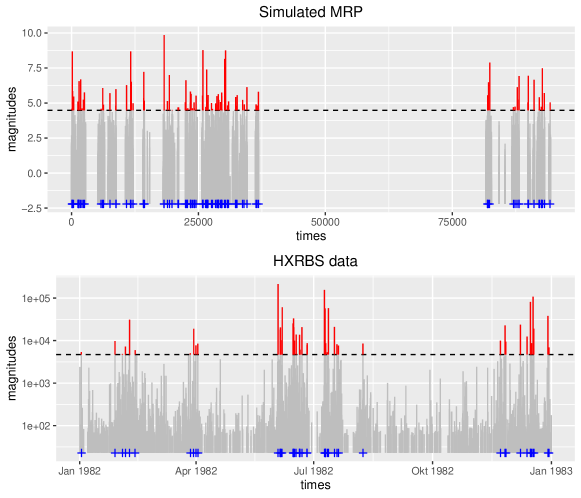
Figure 1: Exceedances (red) and times until Exceedance (durations between blue crosses) for a given threshold $\ell$ (dashed line). Upper picture: Simulated data with stable distributed waiting times. Lower picture: Solar flares during 1982.

In this article, we restrict ourselves to the uncoupled case, where $W$ and $J$ are independent. Then the two sequences $X(\ell,n)_{n\in\mathbb{N}}$ and $T(\ell,n)_{n\in\mathbb{N}}$ are independent as well. To see why, note that $X(\ell)$ is, in distribution, simply equal to $J-\ell|J>\ell$, independent of any waiting time $W_{k}$.
We assume for the rest of the article, that the magnitudes $(J_{i})_{i\in\mathbb{N}}$ belong to the the max-domain of attraction of some non-degenerate distribution. This means there exist $a_{n}>0$ and $d_{n}\in\mathbb{R}$ such that

$$a_{n}^{-1}(J_{1}\vee\ldots\vee J_{n}-d_{n})\Rightarrow A\text{ as }n\rightarrow\infty.$$ (1)

Hence, the distribution of $A$ is a generalized extreme value distribution (GEV) whose distribution function is given by

$$F(x;\xi)=\begin{cases}\exp(-(1+\xi x)_{+}^{-1/\xi})&\xi\neq 0\\ \exp(-\exp(-x))&\xi=0\end{cases}$$

where $(.)_{+}:=\max\{0,.\}$.

The GEV is subdivided into the Gumbel ($\xi=0$), the Weibull ($\xi<0$) and the Fréchet ($\xi>0$) family of distributions.

Figure 1 shows a simulated dataset in the top panel, where $W$ has a stable distribution with tail parameter $\beta=$ 0.8 (and skewness $1$ and location $0$), and where $J$ is from a standard Gumbel distribution. In the bottom panel, we plot a time series of solar flare intensities derived from a NASA dataset (Dennis et al., 1991) which we will later examine more closely (see Section 7). Clearly, the simulated data exhibit long intervals without any events, whereas in the real-world dataset events appear continuously. The threshold exceedances, however, appear to have visually similar statistical behaviour in both models. Observations below a threshold are commonly discarded in Extreme Value Theory (POT approach); likewise, the CTRE model interprets these observations as noise and discards them.

2.2 Scaling limit of Exceedance Times

In this section we state and prove the key theorem, which is founded on the concept of regular variation.

Theorem:

For the magnitudes $J_{k}$, let assumption (1) hold. Furthermore, let the waiting times $W_{k}$ be in the domain of attraction of a positively skewed sum-stable law with stability parameter $0<\beta<1$; more precisely,

$$\frac{W_{1}+\ldots+W_{n}}{b(n)}\Rightarrow D,\quad n\to\infty$$ (2)

for a function $b(n)$ which is regularly varying at $\infty$ with parameter $1/\beta$, and where $\mathbf{E}[\exp(-sD)]=\exp(-s^{\beta})$, $s>0$. Write $p_{\ell}:=\mathbf{P}(J>\ell)$. Then the weak convergence

$$\frac{T(\ell)}{b(1/p_{\ell})}\Rightarrow Z_{\beta}\quad\text{ as }\quad\ell\uparrow x_{R}$$

holds, where the Mittag-Leffler random variable $Z_{\beta}$ is defined on the positive real numbers via

$$\mathbf{E}[\exp(-sZ_{\beta})]=\frac{1}{1+s^{\beta}}.$$

Proof of Theorem: Due to assumption (1)

$$P\left(\frac{J_{1}\vee\ldots\vee J_{\lfloor c\rfloor}-d(c)}{a(c)}\leq x\right) \rightarrow F(x;\xi)$$

$$\Longleftrightarrow F_{J}(xa(c)+d(c))^{\lfloor c\rfloor} \rightarrow F(x;\xi)$$

$$\Longleftrightarrow \lfloor c\rfloor\log F_{J}(\ell_{c}) \rightarrow\log F(x;\xi)$$

as $c\rightarrow\infty$, for any $x$ from the support of $F(x;\xi)$, with $\ell_{c}:=xa(c)+d(c)$. Furthermore, since $\log(1-x)\sim-x$ for small $x$ it follows

$$c\cdot p(\ell_{c})\rightarrow-\log F(x;\xi)\quad\text{ as }c\rightarrow\infty,$$

with $p(\ell_{c}):=1-F(\ell_{c})$. Due to $\tau(\ell_{c})\sim{\rm Geo}(p(\ell_{c}))$ and above equation, it follows that $\tau(\ell_{c})/c$ converges to an exponential random variable,

$$\frac{\tau(\ell_{c})}{c}\Rightarrow E\quad\text{ as }c\rightarrow\infty$$

with inverse mean $\lambda:=-\log F(x;\xi)$. Due to

$$S(c):=\sum_{i=1}^{\lfloor c\rfloor}\frac{W_{i}}{b(c)}\Rightarrow D\quad\text{ as }c\rightarrow\infty,$$

it follows with Gnedenko’s transfer theorem (see Gnedenko (1983)), that

$$\sum_{i=1}^{\tau(\ell_{c})}\frac{W_{i}}{b(\ell_{c})}\Rightarrow Z\quad\text{ as }c\rightarrow\infty,$$

where the distribution of $Z$ has the characteristic function

$$\Psi(s) =\int_{0}^{\infty}(\Phi_{D}(s))^{y}F_{E}(dy)=\frac{1}{1-\log(\Phi_{D}(s))/\lambda}$$

$$=\frac{1}{1+s^{\beta}\lambda^{-1}}=\frac{1}{1+(s\lambda^{-1/\beta})^{\beta}}$$

where $\Phi_{D}(s)=\exp(-s^{\beta})$ is the Laplace transform of $D$ and $F_{E}(dy)$ is the distribution function of $E$. Hence, $Z$ is Mittag-Leffler distributed with scale parameter $\lambda^{-1/\beta}$. Rewriting

$$\sum_{i=1}^{\tau(\ell_{c})}\frac{W_{i}}{b(1/p(\ell_{c}))}=\left(\sum_{i=1}^{\tau(\ell_{c})}\frac{W_{i}}{b(c)}\right)\frac{b(c)}{b(1/p(\ell_{c}))}$$

and

$$\frac{b(c)}{b(1/p(\ell_{c}))}=\frac{b(c)}{b(c/(p(\ell_{c})c))}\sim(p(\ell_{c})\cdot c)^{1/\beta}\rightarrow\lambda^{1/\beta}\text{ as }c\rightarrow\infty,$$

the second factor converges to $\lambda^{1/\beta}$, and it follows that $Z\sim{\rm ML}(\beta,1)$. Since $c\rightarrow\infty$ is equivalent to $\ell\uparrow x_{R}$, the assertion follows with $\ell:=\ell_{c}$ and $p_{\ell}:=p(\ell_{c})$.

For a scale parameter $\sigma>0$, we write ${\rm ML}(\beta,\sigma)$ for the distribution of $\sigma Z_{\beta}$. The Mittag-Leffler distribution with parameter $\beta\in(0,1]$ is a heavy-tailed positive distribution for $\beta<1$, with infinite mean. However, as $\beta\uparrow 1$, ${\rm ML}(\beta,\sigma)$ converges weakly to the exponential distribution ${\rm Exp}(\sigma)$ with mean $\sigma$. This means that although its moments are all infinite, the Mittag-Leffler distribution may (if $\beta$ is close to 1) be indistinguishable from the exponential distribution, for the purposes of applied statistics.

We caution the reader that, somewhat confusingly, there is another distribution called the “light-tailed” Mittag-Leffler distribution. This is in fact the limiting distribution of the renewal process $N(t)$ above (see Meerschaert and Scheffler (2004)). For a detailed reference on the Mittag-Leffler distribution, see e.g.  Haubold et al. (2011), and for algorithms, see e.g. the R package MittagLeffleR (Gill and Straka, 2017).

Remark:

If $\beta=1$, the result of the Theorem above is standard, see Equation (2.2) in Gut and Hüsler (1999). In Anderson (1987) a similar result is shown with a different choice of scaling constant. Meerschaert and Stoev (2008) proved a limit theorem for the maxima of iid random variables separated by infinite mean waiting times. They also show that the hitting time of the limit process is Mittag-Leffler distributed. Basrak and Špoljarić (2015) describe the asymptotic distribution, under similar assumptions, of all upper orders statistics of the maximum process using point processes.

Remark:

When $0<\beta<1$, the renewal process $N(t)$ is not stationary, and hence the results by Hsing et al. (1988) on the exceedances of stationary sequences do not apply.

3 Statistical Inference

3.1 Mittag-Leffler Stability Plots

We assume a dataset of the form $\{(t_{i},x_{i}),i\in I\}$, where $t_{i}$ are timestamps and $x_{i}$ are magnitudes. In this article, we focus on modelling the distribution of threshold exceedance times rather than the exceedances themselves. For the latter, see the POT approach (Beirlant et al., 2006, p. Ch.5.3; Coles, 2001, p. Ch.4.; Davison and Smith, 1990; Embrechts et al., 2013 Ch. 6.5.; Leadbetter, 1991; Smith, 1984). With the previous section setting the stage, we assume that only the large magnitudes (or “shocks”) follow a MRP. The smaller magnitudes are possibly nuisance data that may be irrelevant with respect to the modelling of extremes and their waiting times. Accordingly, we assume a threshold $\ell$, and discard all data where $x_{i}\leq\ell$, yielding the thresholded dataset $\{(t^{(\ell)}_{i},x^{(\ell)}_{i}):i\in I(\ell)\}$, with $x^{(\ell)}_{i}=x_{i}-\ell$, where $I(\ell):=\left\{i\in I:x_{i}\geq\ell\right\}\subseteq I$.

However, this raises the question of how high or low the threshold should be chosen. Recall that with the POT method for the modelling of extremes, the distribution of the thresholded exceedances converges to a GPD, and the threshold must be chosen high enough so that the exceedances fit a GPD well. The threshold choice translates into a bias-variance trade-off: low thresholds yield more data to fit a GPD (low variance), but the distribution of exceedances may deviate from a GPD distribution (high bias); and high thresholds present the opposite scenario. It is understood, however, that there is a range of threshold values that ought to yield similar GPD parameter estimates. In other words, plots of threshold vs. parameter estimate ought to exhibit that parameter estimates are stable with respect to the choice of threshold.

For inter-exceedance times (IETs), the same idea applies. By the Theorem, the inter-exceedance times converge to a Mittag-Leffler distribution (MLD), and importantly, the tail parameter $\beta$ is independent of (or stable with respect to) the choice of threshold. For high thresholds, the IET distribution may fit an MLD well, but few IETs may be left for a fit (high variance). For low thresholds, their distribution may be not well represented by an MLD; or, too many events may be interpreted as shocks, resulting in a biased estimate of the parameters of the limiting MLD. If we had MRP data $\{(W_{i},J_{i}):i\in I\}$ as defined in Section 2.1, we could apply any tail (and scale) estimator such as e.g. Hill’s estimator (Hill, 1975) to the $W_{i}$ and thus infer the distribution of inter-exceedance times. However, in real-world datasets, the MRP assumption is too strong for low thresholds. The unknown data generating process is likely more complex, with dependencies or multiple data generating mechanisms at low thresholds and structures that may vanish for higher thresholds. Fitting only the IETs means that the iid assumption applies to exceedances and IETs only.

For high thresholds where few IETs are left, estimating a tail parameter by fitting a MLD has advantages over e.g. the Hill estimator: since the underlying distribution of IETs is a MLD, the fits are more accurate. Figure 2 shows Hill plots for 200 IETs, for two Mittag-Leffler datasets of sizes 200 and 10000 (and an irrelevant distribution of magnitudes). Clearly the variance is too high to give useful estimates. For corresponding fits based on the assumption of a Mittag-Leffler distribution, see Figure 5, top row, yielding more reliable predictions (more discussion further below).

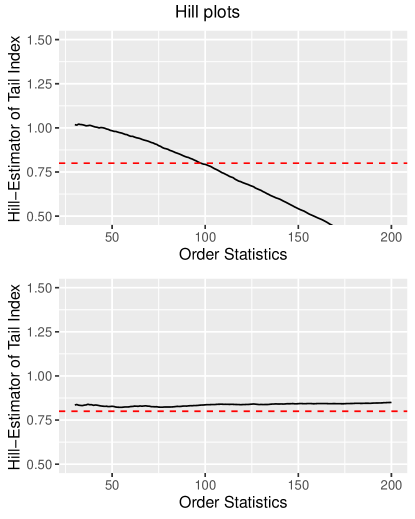
Figure 2: Hill plots for m=100 simulated Mittag-Leffler datasets with true tail 0.8 and sample size 200 (first panel) and 10000 (second panel), with number of upper order statistics r on which the Hill estimator is based on the x-axis. The grey thin lines are the Hill plots for the different simulation runs and the dark lines are their means. The red dotted line shows the true tail parameter.

3.2 Fitting Mittag-Leffler Distributions

Historically, the first method proposed for the estimation of the Mittag-Leffler distribution parameters was the fractional moment estimator by Kozubowski (2001). Unlike the first moments, the fractional moments of order $p$ for $p<\beta$ exist and are tractable. One drawback of this method is that constant priors for the tail parameter are needed for the calculation of the estimates. Cahoy et al. (2010) proposed a moment estimator of the log-transformed data, which does not require any prior. Furthermore, they performed simulation studies illustrating that the log-Moment outperforms the fractional moment estimator with respect to bias and root mean squared error (RMSE).

The Maximum Likelihood Estimator (MLE) for the MLD is not straightforward to implement, since the MLD density admits no closed form analytical expression. In the R Package MittagLeffleR (Gill and Straka, 2017), MLE is implemented via numerical optimization. The MLE slightly outperforms the log-Moment estimator regarding bias and RMSE for big enough sample sizes, but is computationally very intensive. Figure 3 shows that both estimators perform well, even for small sample sizes. For smaller tails both estimators show an increasing RMSE for the scale estimation due to an increasing variance. This results from the fact that in case of very small tails, single very large values can occur.

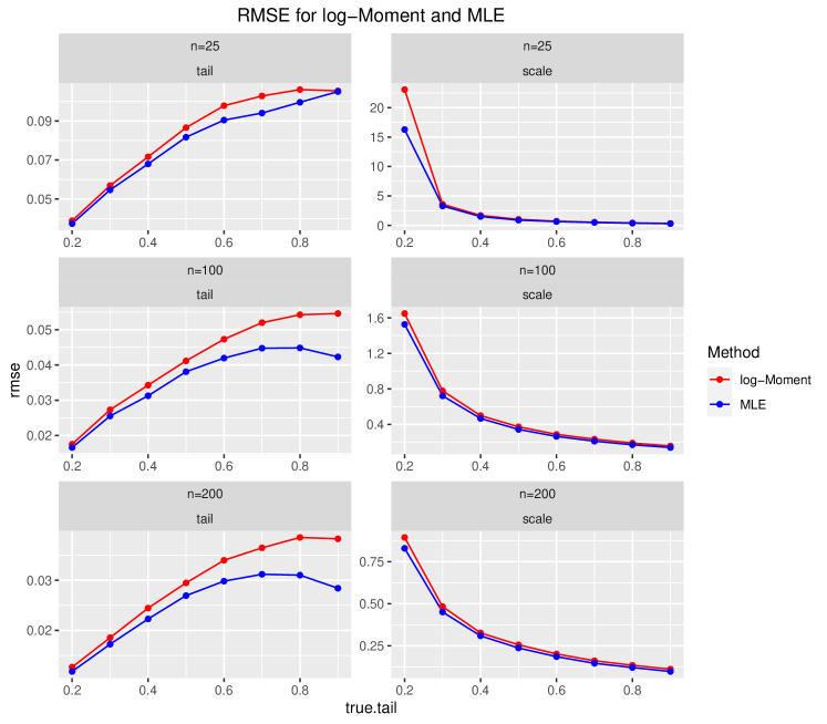
Figure 3: RMSE for the estimation of tail (left column) and scale (right column) parameters via log-Moment estimator and MLE of a Mittag-Leffler sample with varying sample size n=25, 100, 200, varying tails on the x-axis and fixed scale equal to one, based on 5000 simulation runs.

With the above comparisons of estimators for the MLD in mind, we propose to use the log-Moment estimator, or the MLE when computational resources are not an issue.

3.3 Weighing the evidence for non-exponential inter-arrival times

Since the exponential distribution is nested in the Mittag-Leffler family of distributions, a Likelihood-ratio Test (LRT) seems to be an appropriate way to choose between a model with exponential and Mittag-Leffler inter-exceedance times. Although the two models are nested, the asymptotic distribution is not $\chi^{2}_{1}$-distributed, and Wilk’s Theorem does not hold: under $H_{0}$, the parameter $\beta$ of Mittag-Leffler distribution is equal to $1$, and hence lies on the boundary of the parameter space $(0,1]$. Instead, a valid approach is a bootstrapped Likelihood-ratio test (see e.g. Davison et al., 1997). Figure 4 displays the (simulated) power for the bootstrapped LRT for Mittag-Leffler distributions with varying tail parameters based on 1000 simulation runs. As expected, the power decreases for tail parameters close to one, since the Mittag-Leffler distribution converges as $\beta\uparrow 1$ to an exponential distribution; it becomes hard to differentiate a Mittag-Leffler distribution from an exponential.

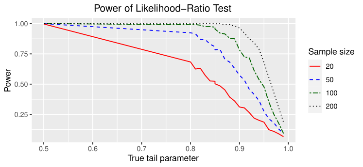
Figure 4: Power for bootstrapped LRT for different sample sizes, varying tails and scale parameter equal to 1.

3.4 Algorithm for the inference on inter-exceedance times

The Theorem in Section 2.2 implies that for a high threshold $\ell$ we may approximate the distribution of $T(\ell)$ with an ${\rm ML}(\beta,b(1/p_{\ell}))$ distribution, where the function $b(c)$ varies regularly at $\infty$ with parameter $1/\beta$. Building on the POT (Peaks-Over-Threshold) method, we propose the following estimation procedure for the distribution of inter-exceedance time $T(\ell)$:

1. Extract the $K$ largest order statistics (i.e. the $K$ largest values, where e.g. $K=300$) $x_{(1)},\ldots,x_{(K)}$ together with their timestamps $t_{(1)},\ldots,t_{(K-1)}$.

2. Choose a minimum number of exceedances $K_{0}\leq K$, e.g. $K_{0}=5$, and for each $k$ ranging from $K_{0}$ to $K$:

   1. extract the set $\mathcal{T}_{k}$ of exceedance times between the magnitudes exceeding the threshold $X_{(k)}$

   2. fit a Mittag-Leffler distribution to $\mathcal{T}_{k}$, resulting in the parameter estimates $\hat{\beta}_{k}$ and $\hat{\sigma}_{k}$.

3. Plot $k$ vs. $\hat{\beta}_{k}$. To the right ($k\uparrow K$, low threshold), the asymptotics are off and bias is high. To the left ($k\downarrow K_{0}$, high threshold), data is scarce and variance is high. In the middle, look for a region of stability for a parameter estimate $\hat{\beta}$. Choose as $\hat{\beta}$ a representative value from this region.

4. Plot $k$ vs. $k^{1/\hat{\beta}}\hat{\sigma}_{k}$. Again, choose a region of stability and a representative $\hat{\sigma}_{0}$ from that region.

The inferred values $\hat{\beta}$ and $\hat{\sigma}_{0}$ can then be interpreted as follows: Setting the threshold at $X_{(k)}$, the threshold exceedance times follow a Mittag-Leffler distribution with shape parameter $\hat{\beta}$ and scale parameter $\hat{\sigma}_{0}k^{-1/\beta}$.

To clarify Step 4: Recall that by the theorem, $\sigma_{k}/b(1/p_{\ell})$ is expected to stabilize around a constant as $k$ decreases. Since $b$ is regularly varying with parameter $1/\beta$, we have $b(1/p_{\ell})=p_{\ell}^{-1/\beta}/L(1/p_{\ell})$ for some slowly varying function $L$. Approximating $p_{\ell}$ by $\hat{p}_{\ell}:=k/n$, we have

$$\text{const}\approx\sigma_{k}/b(1/p_{\ell})=\sigma_{k}\times p_{\ell}^{1/\beta}L(1/p_{\ell})\approx\sigma_{k}\times k^{1/\beta}n^{-1/\beta}L(n/k)$$

Assuming that the variation of $L(n/k)$ is minor, we can hence see that $\sigma_{k}k^{1/\beta}$ stabilizes.

Remark:

We approximated $p_{\ell}$, the probability that an event is larger than $l$, by its relative frequency. One could also approximate this tail probability via the GPD distribution fitted to the exceedances.

For computationally efficient estimates of the Mittag-Leffler parameters we have used the method of log-transformed moments. This estimation method provides point estimates as well as confidence intervals based on sampling variance (Cahoy, 2013), and has been implemented in the R software package MittagLeffleR (Gill and Straka, 2017). The stability plots for $\hat{\beta}$ and $\hat{\sigma}_{0}$ can be furnished with these confidence intervals, see e.g. Figure 10, to produce (non-simultaneous) confidence bands. These stability plots were produced with the R package CTRE (Hees and Straka, 2018). We have verified the validity of our estimation algorithm via simulations, see Section 4.

4 Simulation Study

To test our inference method via stability plots, we have simulated $m=100$ datasets with $n=10000$ independent waiting time and magnitude pairs $(W_{k},J_{k})$ for waiting times that follow

1. a stable distribution,

2. a Pareto distribution and

3. an exponential distribution.

The magnitudes are in all scenarios standard Gumbel distributed. In order to have exact analytical values available for $\beta$ and $\sigma_{0}$, a distribution for $W_{k}$ needs to be chosen for which $b(n)$ from (2) is known.

Case (i): For (i) we choose $W_{k}\stackrel{{\scriptstyle d}}{{=}}D$, where $D$ is as in (2), then due to the stability property we have the equality of distribution $W_{1}+\ldots+W_{n}\stackrel{{\scriptstyle d}}{{=}}b(n)D$, for $b(n)=n^{1/\beta}$. Using the parametrisation of Samorodnitsky and Taqqu (1994), a few lines of calculation (see e.g. the vignette on parametrisation in Gill and Straka, 2017) show that $D$ must have the stable distribution $S_{\beta}(\cos(\pi\beta/2)^{1/\beta},+1,0)$, which is implemented in the R package stabledist by Wuertz et al. (2016). By the Theorem, the distribution of $T(\ell)$ is approximately

$${\rm ML}(\beta,p_{\ell}^{-1/\beta})={\rm ML}(\beta,k^{-1/\beta}n^{1/\beta}),$$

which means $\sigma_{0}=n^{1/\beta}$.

Case (ii): In the Pareto example we choose $P(W>t)=Ct^{-\beta}$ with $C=(1/\Gamma(1-\beta))^{1/\beta}$. We have chosen $\beta=0.8$ in both cases (i) and (ii).

Case (iii): We choose exponentially distributed waiting times with a rate parameter of $1$.

Figure 5 shows the graphical “stability plots” for the estimation of the tail parameter, where

• rows correspond to cases (i), (ii) and (iii), and

• columns correspond to estimators (log-Moment estimator, Maximum-Likelihood).

We plot the tail parameter estimates $\hat{\beta}(k)$ against $k$ for each of the $m=100$ simulation runs. Thin grey lines represent individual simulation runs, and the thicker black line is their mean. Recall that $k$ is the index of the order statistics of $J_{k}$ at which the threshold $\ell$ is placed.

The performance of log-Moment and Maximum-Likelihood estimators for the tail resp. the scale parameter is shown in Figure 5 resp. 6. Both estimators show good performance, with a slight advantage for the Maximum-Likelihood estimator. This advantage is paid for with a higher computational cost. Moreover, the bottom row in Figure 5 shows clearly that the log-Moment and Maximum-Likelihood estimators generalize to the exponential case ($\beta=1$) whereas the Hill-estimator would not.
Notice that any data below a certain threshold is discarded in our approach and hence need not satisfy the iid assumption. In our simulation study we only simulated data from iid sequences of $(W_{k})_{k\in\mathbb{N}}$; in real data situations it is likely that there are dependencies or more complex data generating processes which vanish for higher thresholds. We only need the exceedances and IETs to be iid.

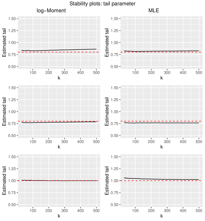
Figure 5: Stability Plots for m=100 simulation runs for stable distributed waiting times with a tail parameter of 0.8 (top row), Pareto distributed waiting times with tail parameter 0.8 (middle row) and exponentially distributed waiting times (lower row). Left column: log-Moment estimator, right column: MLE. The grey thin lines are the stability plots for the different simulation runs and the dark lines are their means. The red dotted line shows the true tail parameter.

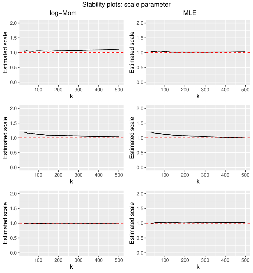
Figure 6: Stability Plots for m=100 simulation runs for stable distributed waiting times with a tail parameter of 0.8 (top row), Pareto distributed waiting times with tail parameter 0.8 (middle row) and exponentially distributed waiting times (lower row). Left column: log-Moment estimator, right column: MLE. The grey thin lines are the stability plots for the different simulation runs and the dark lines are their means. The red dotted line shows the true scale parameter.

5 Data example

We now want to apply the proposed method to a real data example, the solar flare data which was already mentioned in Section 1 and can be seen in Figure 1. The data were extracted from the “complete Hard X Ray Burst Spectrometer event list”, a comprehensive reference for all measurements of the Hard X Ray Burst Spectrometer on NASA’s Solar Maximum Mission from the time of launch on Feb 14, 1980 to the end of the mission in Dec 1989. 12,772 events were detected, with the “vast majority being solar flares”. To assure stationarity and due to missing values during the years 1983 and 1984, we based our analysis just on the year 1982, in which 2,488 events happened. The list includes the start time, peak time, duration, and peak rate of each event. We have used “start time” as the variable for event times, and “peak rate” as the variable for event magnitudes.

Before we apply the approach described in Section 5 to the solar flare data, we first have to check if all model assumptions are fulfilled. The CTRE model is based on three main assumptions, which are repeated below. For each assumption, we suggest one means of checking if it holds:

iid:

After removing the “noise observations” below the smallest threshold $\ell_{0}$, the pair sequence $(T(\ell_{0},i),X(\ell_{0},i))$ is iid. An indication if this is true is given by an auto-correlation plot. Since we are expecting the inter-exceedance times to be Mittag-Leffler distributed and hence to have infinite mean but finite log-moments, we first take the logarithms of the times.

Uncoupled:

Each $T(\ell,i)$ is independent of each $X(\ell,i)$. We propose an empirical copula plot to check for any dependence.

${\rm ML}(\beta,\sigma)$ distribution of $T(\ell,i)$:

Apply a cutoff at the lowest threshold $\ell_{0}$, extract the threshold crossing times, and create a QQ Plot for the Mittag-Leffler distribution. Use a Log-moment estimate of the tail parameter for the theoretical / population quantiles of the plot.

Remark:

The ACF plots of course can just give an indication whether there are dependencies, since they actually just measure linear dependencies. Furthermore, if one calculates the ACF for the logarithmic inter-exceedance times, the ACF indicates on the original scale a multiplicative dependence.

Figures 7, 8 and 9 show the diagnostic plots for a minimum threshold chosen at the 100th order statistic. There is some residual autocorrelation for the sequence of threshold exceedance times that is not accounted for by the CTRE model.

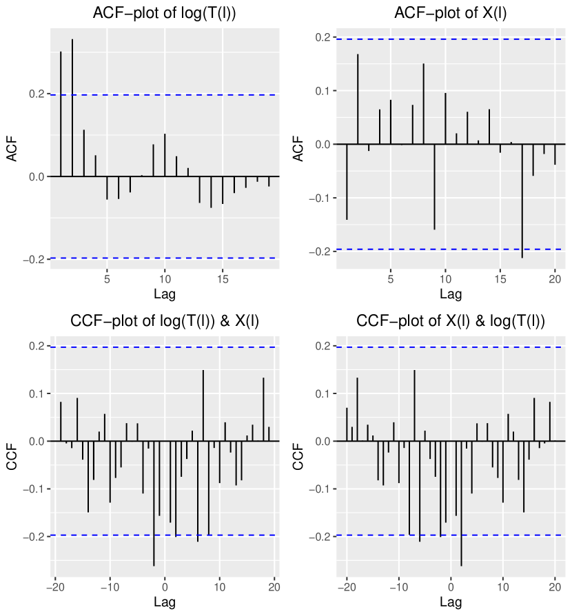
Figure 7: Diagnostic plots for the solar flare data based on the 100 upper order statistics: auto-correlation and cross-correalation function.

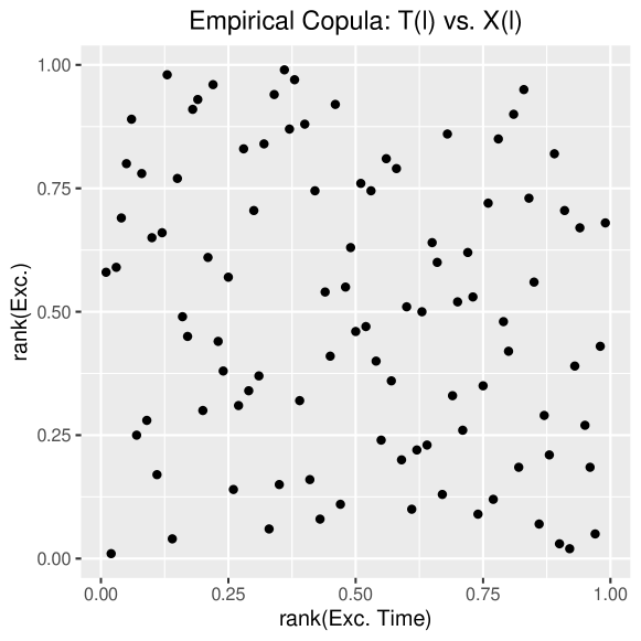
Figure 8: Diagnostic plots for the solar flare data: empirical copula.

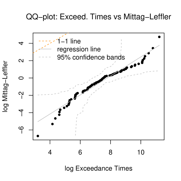
Figure 9: Diagnostic plots for the solar flare data: QQ Plot.

Figure 10 shows the stability plots for the solar flare data, on the left for the tail parameter and on the right for the scale parameter. The dark grey ranges correspond to 95% confidence intervals, which are derived from the asymptotic normality of the Log-moment estimators (Cahoy, 2013) and the $\delta$-method (Gill and Straka, 2017); dashed lines show the deduced true values of $\beta$ resp. $\sigma_{0}$. The stability plot for the tail stabilizes nicely around 0.9 (dashed line), while the scale parameter stabilizes less obviously near $3\times 10^{7}$ (dashed line). The growth of the scale parameter for lower threshold appears to be closer to linear in $p_{\ell}$, rather than proportional to $p_{\ell}^{1/0.9}$ as suggested by the Mittag-Leffler fits. The reason for this is likely that the overall goodness of fit as compared to an exponential distribution is improved due to the peaked shape of the Mittag-Leffler distribution near $0$, rather than its tail behaviour at $\infty$. The reported fit should hence come with the caveat that a Mittag-Leffler distribution models exceedance times well only up to certain time-scales. More research is needed into the modelling of scale transitions, where inter-exceedance times appear to have different power laws across different time scales.

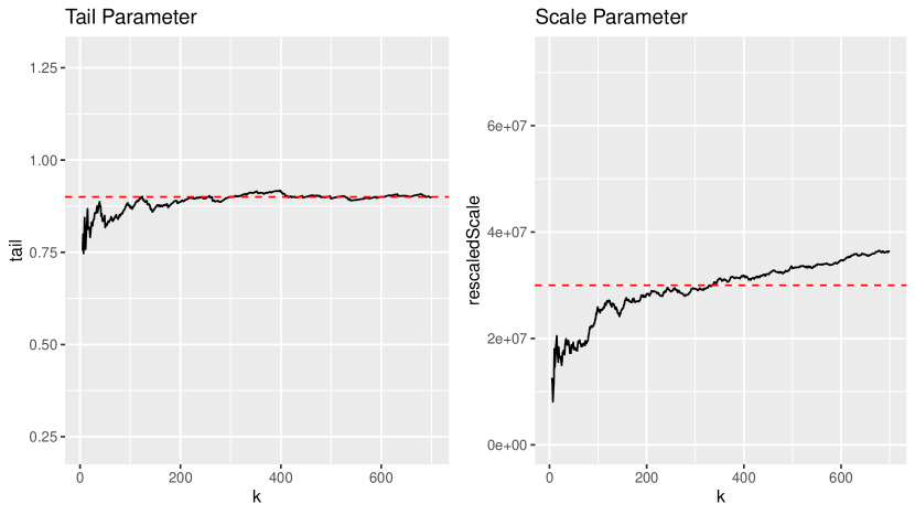
Figure 10: Stability plots for the tail and scale parameter of the Mittag-Leffler distribution of the Solar Flare dataset. Dotted horizontal lines are at $\beta=0.9$ and $\sigma_{0}=3\times 10^{7}$ seconds $\approx 0.95$ years.

The fit with a Mittag-Leffler distribution ($\beta=0.9$) seems to be good (see Figure 9), although there are signs that the power-law tail tapers off for very large inter-threshold crossing times. There is no apparent dependence between threshold exceedance times and event magnitudes seen in the copula plot (see Figure 8). We also conduct a bootstrapped LRT for the null hypothesis of exponentially distributed inter-arrival times and received a $p$-value of $p<0.01$.

6 Predicting the time of the next threshold crossing

According to Figure 10, for a threshold $\ell$ at the $k$-th order statistic, the estimated threshold exceedance time distribution is approximately

$$T(\ell)\sim{\rm ML}(\hat{\beta},k^{-1/\hat{\beta}}\hat{\sigma}_{0}),$$

where $\hat{\beta}=0.9$ and $\hat{\sigma}_{0}=3.0\times 10^{7}{\rm sec}$. Unlike the exponential distribution, the Mittag-Leffler distribution is not memoryless, and the probability density of the time $t$ until the next threshold crossing will depend on the time $t_{0}$ elapsed since the last threshold crossing. This density is approximately equal to

$$p(t|\beta,\sigma_{0},\ell,t_{0})=\frac{f(t+t_{0}|\beta,k^{-1/\beta}\sigma_{0})}{\mathbf{P}[T_{\ell}>t_{0}]}$$

where $f(\,\cdot\,|\beta,k^{-1/\beta}\sigma_{0})$ is the probability density of ${\rm ML}(\beta,k^{-1/\beta}\sigma_{0})$. The more time has passed without a threshold crossing, the more the probability distribution shifts towards larger values for the next crossing (see Figure 11, left panel). The hazard rate

$$h(t)=\frac{f(t|\beta,k^{-1/\beta}\sigma_{0}))}{\int_{t}^{\infty}f(\tau|\beta,k^{-1/\beta}\sigma_{0}))\,d\tau}$$

approximates the risk of a threshold crossing per unit time, and is a decreasing function for the Mittag-Leffler distribution.

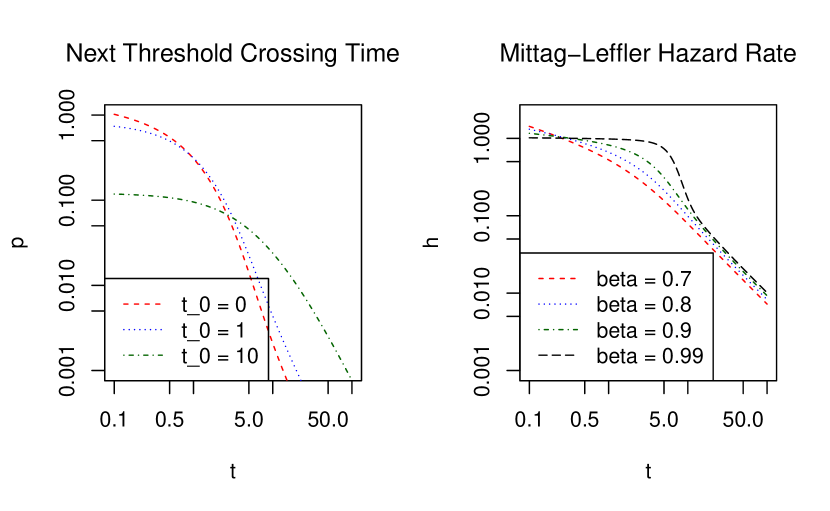
Figure 11: Left: Conditional distribution of time until next threshold crossing, depending on elapsed time $t_{0}$ since last crossing ($\beta=0.9$, $\sigma_{0}=1$). Right: Hazard rate depending on tail parameter $\beta$.

The closer $\beta$ is to $1$, the more the hazard rate mimics that of an exponential distribution (a constant function, see Figure 11, right panel).

7 Discussion & Conclusion

We proposed a new model and inference procedure for the inter-exceedance times of “bursty” time series, which have been studied intensively in statistical physics. Burstiness is characterized by power-law waiting times between events, and we have shown that the Mittag-Leffler distribution arises naturally as a scaling limit for the inter-exceedance times of high thresholds. Moreover, we have derived the following non-linear scaling behaviour: $\sigma\sim p_{\ell}^{-1/\beta}$, where $\sigma$ is the scale parameter of the distribution of threshold exceedance times, $p_{\ell}$ is the fraction of magnitudes above the threshold $\ell$, and $\beta$ the exponent of the power law. This “anomalous” scaling behaviour in the bursty setting entails two phenomena:

1. a heavy tail of the inter-arrival time distribution of threshold crossings (long rests), and

2. a high propensity for more threshold crossing events immediately after each threshold crossing event (bursts).

The Mittag-Leffler distribution captures both phenomena, due to its heavy tail as well as its stretched exponential (peaked) asymptotics for small times. It generalizes the exponential distribution, and in the solar flare data example, this generalization is warranted, because the likelihood-ratio test is strongly significant.

When we introduced the CTRE model, we assumed that all events are iid. This assumption is likely sufficient but not necessary for our limit theorem to hold. Moreover, any data below a (minimum) threshold $\ell_{0}$ is discarded for CTREs, and hence need not satisfy the iid assumption. For the purposes of statistical inference, we merely require that the IETs are iid.

The CTRE approach to model “non-Poissonian” threshold crossing times should be contrasted with the well-documented approach of clusters of extremes, see e.g. Ferro and Segers (2003). When the underlying stochastic process is stationary, the exceedances of high thresholds form, asymptotically, a Cluster Poisson Process. This result was established in (Hsing et al., 1988). In the setting of this article, however, clustering-like dynamics occur due to the non-stationarity of the underlying renewal-reward process, which has infinite-mean renewal times. Hence CTRE and Cluster Poisson Process should not be viewed as competing methods, as the underlying data generating processes are quite different. To differentiate between the two models we use the term bursty which is standard in the context of heavy-tailed inter-arrival times in the physics community (e.g. Barabási, 2005; Karsai et al., 2012; Vajna et al., 2013; Vasquez et al., 2006)). In weighing the evidence for either of the two data generating processes, criteria could be developed, based e.g. on measures of surprise (Lee et al., 2015), which may prove to be valuable for future applied statisticians.

Finally, we note that assuming a purely scale-free pattern for event times may be too rigid an assumption, which unnecessarily limits the applicability of CTREs. Often, the heavy-tailed character of the inter-arrival time distribution holds at short to intermediate time scales, and is truncated (or tempered, reverting to an exponential distribution) at very long time scales (see e.g. Meerschaert et al., 2012; and Aban et al., 2006). In such situations, a “tempered” Mittag-Leffler distribution may provide a better fit, which we aim to introduce in follow-up work.

References

Aban, I.B., Meerschaert, M.M., Panorska, A.K., 2006. Parameter estimation for the truncated pareto distribution. J. Am. Stat. Assoc. 101, 270–277.

Anderson, K.K., 1987. Limit Theorems for General Shock Models with Infinite Mean Intershock Times. J. Appl. Probab. 24, 449–456.

Bagrow, J.P., Brockmann, D., 2013. Natural emergence of clusters and bursts in network evolution. Phys. Rev. X 3, 1–6.

Barabási, A.L., 2005. The origin of bursts and heavy tails in human dynamics. Nature 435, 207–211.

Basrak, B., Špoljarić, D., 2015. Extremes of random variables observed in renewal times. Stat. Probab. Lett. 97, 216–221.

Beirlant, J., Goegebeur, Y., Segers, J., Teugels, J., 2006. Statistics of extremes: theory and applications. John Wiley & Sons.

Benson, D.A., Schumer, R., Meerschaert, M.M., 2007. Recurrence of extreme events with power-law interarrival times. Geophys. Res. Lett. 34.

Cahoy, D.O., 2013. Estimation of Mittag-Leffler Parameters. Commun. Stat. - Simul. Comput. 42, 303–315.

Cahoy, D.O., Uchaikin, V.V., Woyczynski, W.A., 2010. Parameter estimation for fractional Poisson processes. J. Stat. Plan. Inference 140, 3106–3120.

Coles, S., 2001. An Introduction to Statistical Modelling of Extreme Values. Springer-Verlag, London.

Davison, A.C., Hinkley, D.V., others, 1997. Bootstrap methods and their application. Cambridge university press.

Davison, A.C., Smith, R.L., 1990. Models for exceedances over high thresholds. Journal of the Royal Statistical Society: Series B (Methodological) 52, 393–425.

Dennis, B.R., Orwig, L.E., Kennard, G.S., Labow, G.J., Schwartz, R.A., Shaver, A.R., Tolbert, A.K., 1991. The complete Hard X Ray Burst Spectrometer event list, 1980-1989.

Embrechts, P., Klüppelberg, C., Mikosch, T., 2013. Modelling extremal events: For insurance and finance. Springer Science & Business Media.

Esary, J.D., Marshall, A.W., 1973. Shock Models and Wear Processes 1, 627–649.

Ferro, C.A., Segers, J., 2003. Inference for clusters of extreme values. Journal of the Royal Statistical Society: Series B (Statistical Methodology) 65, 545–556.

Gill, G., Straka, P., 2017. MittagLeffleR: Using the mittag-leffler distributions in r.

Gnedenko, B., 1983. On limit theorems for a random number of random variables, in: Probability Theory and Mathematical Statistics. Springer, pp. 167–176.

Gut, A., Hüsler, J., 1999. Extreme Shock Models. Extremes 2, 295–307.

Haubold, H.J., Mathai, A.M., Saxena, R.K., 2011. Mittag-Leffler Functions and Their Applications. J. Appl. Math. 2011, 1–51.

Hawkes, A.G., 1971. Point spectra of some mutually exciting point processes. J. R. Stat. Soc. Ser. B Stat. Methodol. 438–443.

Hees, K., Scheffler, H.-P., 2018a. On joint sum/max stability and sum/max domains of attraction. Probability and Mathematical Statistics 38.

Hees, K., Scheffler, H.-P., 2018b. Coupled continuous time random maxima. Extremes 21, 235–259.

Hees, K., Straka, P., 2018. CTRE: Thresholding bursty time series.

Hill, B.M., 1975. A simple general approach to inference about the tail of a distribution. The annals of statistics 1163–1174.

Hsing, T., Hüsler, J., Leadbetter, M.R., 1988. On the exceedance point process for a stationary sequence. Probability theory and related fields 78, 97–112.

Karsai, M., Kaski, K., Barabási, A.L., Kertész, J., 2012. Universal features of correlated bursty behaviour. Sci. Rep. 2.

Karsai, M., Kivelä, M., Pan, R.K., Kaski, K., Kertész, J., Barabási, A.L., Saramäki, J., 2011. Small but slow world: How network topology and burstiness slow down spreading. Phys. Rev. E - Stat. Nonlinear, Soft Matter Phys. 83, 1–4.

Kozubowski, T.J., 2001. Fractional moment estimation of linnik and mittag-leffler parameters. Mathematical and computer modelling 34, 1023–1035.

Laskin, N., 2003. Fractional Poisson process. Commun. Nonlinear Sci. Numer. Simul. 8, 201–213.

Leadbetter, M.R., 1991. On a basis for ‘peaks over threshold’modeling. Statistics & Probability Letters 12, 357–362.

Lee, J., Fan, Y., Sisson, S.A., 2015. Bayesian threshold selection for extremal models using measures of surprise. Comput. Stat. Data Anal. 85, 84–99.

Meerschaert, M.M., Nane, E., Vellaisamy, P., 2011. The fractional Poisson process and the inverse stable subordinator. Electron. J. Probab. 16, 1600–1620.

Meerschaert, M.M., Roy, P., Shao, Q., 2012. Parameter estimation for exponentially tempered power law distributions. Commun. Stat. - Theory Methods 41, 1839–1856.

Meerschaert, M.M., Scheffler, H.-P., 2004. Limit Theorems for Continuous-Time Random Walks with Infinite Mean Waiting Times. J. Appl. Probab. 41, 623–638.

Meerschaert, M.M., Sikorskii, A., 2012. Stochastic models for fractional calculus. Walter de Gruyter.

Meerschaert, M.M., Stoev, S.A., 2008. Extremal limit theorems for observations separated by random power law waiting times. J. Stat. Plan. Inference 139, 2175–2188.

Min, B., Goh, K.I., Vazquez, A., 2011. Spreading dynamics following bursty human activity patterns. Phys. Rev. E - Stat. Nonlinear, Soft Matter Phys. 83, 2–5.

Oliveira, J., Barabási, A.L., 2005. Darwin and Einstein correspondence patterns. Nature 437, 1251.

Omi, T., Shinomoto, S., 2011. Optimizing Time Histograms for Non-Poissonian Spike Trains. Neural Comput. 23, 3125–3144.

R Core Team, 2018. R: A language and environment for statistical computing. R Foundation for Statistical Computing, Vienna, Austria.

Samorodnitsky, G., Taqqu, M.S., 1994. Stable Non-Gaussian Random Processes: Stochastic Models with Infinite Variance, Stochastic modeling. Chapman Hall, London.

Shanthikumar, J.G., Sumita, U., 1983. General shock models associated with correlated renewal sequences. J. Appl. Probab. 20, 600–614.

Shanthikumar, J.G., Sumita, U., 1984. Distribution Properties of the System Failure Time in a General Shock Model. Adv. Appl. Probab. 16, 363–377.

Shanthikumar, J.G., Sumita, U., 1985. A class of correlated cumulative shock models. Adv. Appl. Probab. 17, 347–366.

Silvestrov, D.S., 2002. Limit Theorems for Randomly Stopped Stochastic Processes. Springer (Berlin, Heidelberg).

Silvestrov, D.S., Teugels, J.L., 2004. Limit theorems for mixed max-sum processes with renewal stopping. Ann. Appl. Probab. 14, 1838–1868.

Smith, R.L., 1984. Threshold methods for sample extremes, in: Statistical Extremes and Applications. Springer, pp. 621–638.

Stindl, T., Chen, F., 2018. Likelihood based inference for the multivariate renewal hawkes process. Computational Statistics & Data Analysis 123, 131–145.

Vajna, S., Tóth, B., Kertész, J., 2013. Modelling bursty time series. New J. Phys. 15, 103023.

Vasquez, a, Oliveira, J.G., Dezso, Z., Goh, K.-I., Kondor, I., Barabási, A.L., 2006. Modeling bursts and heavy tails in human dynamics. Phys. Rev. E 73, 361271–3612718.

Vazquez, A., Rácz, B., Lukács, A., Barabási, A.L., 2007. Impact of non-poissonian activity patterns on spreading processes. Phys. Rev. Lett. 98, 1–4.

Wheatley, S., Filimonov, V., Sornette, D., 2016. The hawkes process with renewal immigration & its estimation with an em algorithm. Computational Statistics & Data Analysis 94, 120–135.

Wuertz, D., Maechler, M., members., R. core team, 2016. Stabledist: Stable distribution functions.