Completeness and divergence-free behavior of the quasi-normal modes using causality principle

Abstract

A fundamental feature of the quasi-normal modes (QNMs), which describe light interaction with open (leaky) systems like nanoparticles, lies in the question of the completeness of the QNMs representation and in the divergence of their field profile due to their leaky behavior and complex eigenfrequency. In this article, the QNMs expansion is obtained by taking into consideration the frequency dispersion and the causality principle. The derivation based on the complex analysis ensures the completeness of the QNMs expansion and prevents from any divergence of the field profile. The general derivation is tested in the case of a one-dimensional open resonator made of a homogeneous absorptive medium with frequency dispersion given by the Lorentz model. For a harmonic excitation, the result of the QNMs expansion perfectly matches the exact formula for the field distribution outside as well as inside the resonator.

https://doi.org/10.1364/OSAC.1.000340

1 Introduction

Light interaction with nanoparticles enables a wide range of unprecedented applications such as high-resolution spectroscopy, photothermal cancer therapy, optical tweezers, and light steering using metasurfaces [1, 2, 3, 4]. The nanoparticles can be viewed as open resonators that are able to confine light down to subwavelength dimensions. Since the energy can escape towards the surroundings, such open systems are nonconservative and their behavior can be described by quasi-normal modes (QNMs) characterized by complex eigenvalues [5, 6, 7].

The QNMs expansion provides direct physical description and interpretation of the light-particle interaction through the investigation of the resonant modes of the system. In addition, the QNMs expansion may lead to reduced computational efforts since the resonant modes of the system have to be calculated only once and then used to solve the excitation problem by evaluating the contribution of the resonances modes near the excitation frequency. The QNMs approach has shown its relevance in many situations such as the calculation of the effective mode volume for leaky cavities [8] and of the Purcell factor [9], the modeling of light behavior in plasmonic nanoparticles [10, 11], the design of angle-independent spectral filters [12], the scattering matrix calculations [13], the local density of states calculations [14], the modeling of the perturbations of black holes [15], and the list goes on. Moreover, it has been recently demonstrated that the peaks of the extinction spectrum of a scattering particle are associated with its QNMs [16], which cannot be elucidated by the multipolar expansion.

The QNMs expansion suffers however from a longstanding limitation: the complex nature of the eigenvalues $z_{q}$ of open systems results in the divergence of the field outside the resonator, i.e. $e^{iz_{q}|\boldsymbol{r}|}\rightarrow\infty$ when $|\boldsymbol{r}|\rightarrow\infty$. This divergence complicates the normalization of the QNMs since the energy of the modes is unbounded and, more importantly, the QNMs expansion appears to fail in describing the radiation outside the open resonator. Several solutions have been proposed to explicitly mitigate the normalization difficulty for leaky resonators [8, 9, 17]. Other approaches based on the Dyson equation formalism [10] lead to the definition of regularized QNMs from the knowledge of standard QNM inside the resonator, which are then propagated in the background using the Green’s function of the background [18]. The theoretical question of the validity of the QNMs expansion outside the resonator still remains an open problem that doubts the completeness of the QNMs, i.e., the ability of the QNMs to form a complete set of modes to represent the field in the whole space, especially in the case of absorptive and dispersive systems. In Ref. [19], it was suggested that the exponential divergence outside the resonator is attributed to a noncausal flaw in the definition of the QNMs. A recent review could be consulted for an exhaustive discussion on the recent advances in the topic of QNMs expansion [20].

In this article, the QNMs expansion is derived taking into consideration the frequency dispersion and the causality principle. This approach has recently demonstrated the validity of the modal expansion to represent the transient fields produced by a one-dimensional resonator [21]. Herein, it is shown that an additional causality-related phase factor cancels the exponential divergence of the “conventional” QNMs of open systems. Arguments are proposed to support the validity of the expansion on the QNMs of the Green’s function in the whole space. A simple example is presented for a one-dimensional resonator made of a homogeneous absorptive dispersive medium, where the Green’s function of the resonator is expanded using QNMs and then the obtained results are compared to the exact formulation.

2 Causality of the Green’s function

The electromagnetic Green’s function $\mathsf{G}(\boldsymbol{r},\boldsymbol{r}^{\prime};z)$ of a system of permittivity $\varepsilon(\boldsymbol{r},z)$ is defined as the solution of the Helmholtz equation for a point Dirac current source $\delta(\boldsymbol{r}-\boldsymbol{r}^{\prime})$ located at $\boldsymbol{r}^{\prime}$:

$${\color[rgb]{0,0,0}{\boldsymbol{\nabla}\times\boldsymbol{\nabla}\times\mathsf{G}(\boldsymbol{r},\boldsymbol{r}^{\prime};z)-z^{2}\mu_{0}\,\varepsilon(\boldsymbol{r},z)\,\mathsf{G}(\boldsymbol{r},\boldsymbol{r}^{\prime};z)=iz\mu_{0}{\color[rgb]{0,0,0}{\,\mathsf{U}\,\delta(\boldsymbol{r}-\boldsymbol{r}^{\prime})}}\,.}}$$ (1)

Here the following notations have been adopted: $\boldsymbol{r}$ (and $\boldsymbol{r}^{\prime}$) is the position vector of space, $\boldsymbol{\nabla}\times$ is the curl operator, $z$ is the complex frequency, $\mu_{0}$ is the vacuum permeability, and $\mathsf{U}$ is the unit dyadic tensor. The reference system is defined as the infinite media surrounding the resonator and is characterized by the permittivity $\varepsilon_{\text{ref}}(\boldsymbol{r},z)$ and the Green’s function $\mathsf{G}_{\text{ref}}(\boldsymbol{r},\boldsymbol{r}^{\prime};z)$. The difference $\Delta\varepsilon(\boldsymbol{r},z)=\varepsilon(\boldsymbol{r},z)-\varepsilon_{\text{ref}}(\boldsymbol{r},z)$ corresponding to the resonator must be restricted to a bounded domain. Let $\mathsf{G}_{d}(\boldsymbol{r},\boldsymbol{r}^{\prime};z)$ be the “diffracted” (or “difference”) Green’s function, corresponding to the field diffracted by the resonator, defined as the difference

$$\mathsf{G}_{d}(\boldsymbol{r},\boldsymbol{r}^{\prime};z)=\mathsf{G}(\boldsymbol{r},\boldsymbol{r}^{\prime};z)-{\color[rgb]{0,0,0}{\mathsf{G}_{\text{ref}}(\boldsymbol{r},\boldsymbol{r}^{\prime};z)}}\,.$$ (2)

For dispersive media, the permittivities $\varepsilon(\boldsymbol{r},z)$ and $\varepsilon_{\text{ref}}(\boldsymbol{r},z)$ tend to the vacuum one $\varepsilon_{0}$ when the frequency $z\rightarrow\infty$, which in turn suggests when $z\rightarrow\infty$ that

$${\color[rgb]{0,0,0}{\mathsf{G}(\boldsymbol{r},\boldsymbol{r}^{\prime};z)\rightarrow\mathsf{G}_{\text{ref}}(\boldsymbol{r},\boldsymbol{r}^{\prime};z)\rightarrow\mathsf{G}_{0}(\boldsymbol{r}-\boldsymbol{r}^{\prime};z)\>\Longrightarrow\>\mathsf{G}_{d}(\boldsymbol{r},\boldsymbol{r}^{\prime};z)\rightarrow 0\,,}}$$ (3)

where $\mathsf{G}_{0}(\boldsymbol{r}-\boldsymbol{r}^{\prime};z)$ is the free Green’s function in vacuum.

The Fourier transform with respect to the time variable $t$ of the diffracted Green’s function can be defined as

$$\widehat{\mathsf{G}}_{d}(\boldsymbol{r},\boldsymbol{r}^{\prime};t)=\int_{\Gamma_{\eta}}dz\,e^{-izt}\mathsf{G}_{d}(\boldsymbol{r},\boldsymbol{r}^{\prime};z)\,,$$ (4)

where $\Gamma_{\eta}$ is the line parallel to the real axis of complex frequencies $z=\omega+i\eta$, with real part $\omega$ describing $\mathbb{R}$ and imaginary part set to the positive number $\eta$. It is stressed that the integral (4) is well-defined for all $t$, which results from the following property of the permittivity [22]: $\int_{\mathbb{R}}d\omega\big{|}\varepsilon(\omega+i\eta)-\varepsilon_{0}\big{|}<\infty$. The resulting time-dependent function (4) is the Green’s function generated by the spatio-temporal Dirac source $\delta(\boldsymbol{r}-\boldsymbol{r}^{\prime})\delta(t)$.

The evaluation of the integral expression (4) is based on the remark (3) stating that the Green’s functions $\mathsf{G}(\boldsymbol{r},\boldsymbol{r}^{\prime};z)$ and $\mathsf{G}_{\text{ref}}(\boldsymbol{r},\boldsymbol{r}^{\prime};z)$ tend to the free one $\mathsf{G}_{0}(\boldsymbol{r},\boldsymbol{r}^{\prime};z)$ when $z\rightarrow\infty$, so that the exponential behavior of the Green’s functions $\mathsf{G}(\boldsymbol{r},\boldsymbol{r}^{\prime};z)$ and $\mathsf{G}_{\text{ref}}(\boldsymbol{r},\boldsymbol{r}^{\prime};z)$ at high frequencies is governed by $e^{iz|\boldsymbol{r}-\boldsymbol{r}^{\prime}|/c}$, where $c=1/\sqrt{\varepsilon_{0}\mu_{0}}$ is the light velocity in vacuum. Hence it appears reasonable to make this first assumption $(\textrm{I})$:

$$\mathsf{G}_{d}(\boldsymbol{r},\boldsymbol{r}^{\prime};z)\times\,e^{-iz\tau}\,e^{-iz|\boldsymbol{r}-\boldsymbol{r}^{\prime}|/c}\underset{z\rightarrow\infty}{\longrightarrow}0\,.$$ (5)

When the complex frequency $z$ has a positive imaginary part, this assumption is always true for $\tau=0$, while when $z$ has negative imaginary part, it could be necessary to consider the arbitrary small time $\tau>0$, to ensure the vanishing behavior at the limit $z\rightarrow\infty$. A second assumption $(\textrm{II})$ is based on the bound nature of the resonator and of the difference of permittivities $\Delta\varepsilon(\boldsymbol{r},z)=\varepsilon(\boldsymbol{r},z)-\varepsilon_{\text{ref}}(\boldsymbol{r},z)$. Under this condition, it can be assumed that the diffracted Green’s function $\mathsf{G}_{d}(\boldsymbol{r},\boldsymbol{r}^{\prime};z)$, which corresponds to the scattering operator [23], has only a discrete set of resonances $\{z_{q}\}$ located in the lower half plane of complex frequencies (arguments based on the analytic Fredholm theorem [24] or a boundary intergral expression of the scattering operator [23] can be used to support this assumption).

The time-dependent Green’s function (4) is evaluated considering the two following cases. For $t<|\boldsymbol{r}-\boldsymbol{r}^{\prime}|/c$, the line $\Gamma_{\eta}$ is deformed in the upper half plane of complex frequencies, i.e. with positive imaginary part, leading to $\widehat{\mathsf{G}}_{d}(\boldsymbol{r},\boldsymbol{r}^{\prime},t)=0$, since all the Green’s functions are analytic in this domain. For $t>\tau+|\boldsymbol{r}-\boldsymbol{r}^{\prime}|/c$, the line $\Gamma_{\eta}$ is deformed in the lower half plane and the Green’s function is given by the contributions of the set of poles $\{z_{q}\}$:

$$\widehat{\mathsf{G}}_{d}(\boldsymbol{r},\boldsymbol{r}^{\prime},t)=-2i\pi\displaystyle\sum_{\{\text{poles }z_{q}\}}e^{-iz_{q}t}\,\mathsf{G}_{d}^{q}(\boldsymbol{r},\boldsymbol{r}^{\prime},z_{q})\,,$$ (6)

where $\mathsf{G}_{d}^{q}(\boldsymbol{r},\boldsymbol{r}^{\prime},z_{q})$ is the residue of the function $\mathsf{G}_{d}(\boldsymbol{r},\boldsymbol{r}^{\prime},z)$ at its pole $z_{q}$. The application of the residue theorem is justified by the assumption $(\textrm{I})$ that ensures the vanishing value of the integral (4) on an infinite semi-circle in the lower half plane.

Finally, the harmonic Green’s function is retrieved by applying the inverse Laplace transform to the expression (6). For an arbitrary small $\tau$ and for a frequency $z$ with positive imaginary part, the following function is defined:

$$\widetilde{\mathsf{G}}_{\tau,d}(\boldsymbol{r},\boldsymbol{r}^{\prime};z)=\dfrac{1}{2\pi}\displaystyle\int^{\infty}_{\tau+|\boldsymbol{r}-\boldsymbol{r}^{\prime}|/c}dt\>e^{izt}\,\widehat{\mathsf{G}}_{d}(\boldsymbol{r},\boldsymbol{r}^{\prime},t)\,.$$ (7)

Notice that the arbitrary small time $\tau$, introduced to ensure the vanishing limit (5), leads to avoid the time $\tau$ at the start of the time-dependent Green’s function in the Laplace transform (7). It can be shown that the resulting function $\widetilde{\mathsf{G}}_{\tau,d}(\boldsymbol{r},\boldsymbol{r}^{\prime};z)$ tends to the required Green’s function ${\mathsf{G}}_{d}(\boldsymbol{r},\boldsymbol{r}^{\prime};z)$ when $\tau$ tends to zero since the time-dependent function $\widehat{\mathsf{G}}_{d}(\boldsymbol{r},\boldsymbol{r}^{\prime};t)$ is bounded with respect to time $t$. Hence the diffracted Green’s function can be expressed as an expansion of the complex resonances (or QNMs):

$$\mathsf{G}_{d}(\boldsymbol{r},\boldsymbol{r}^{\prime};z)=\displaystyle\lim_{\tau\rightarrow 0}\displaystyle\sum_{\{\text{poles }z_{q}\}}\dfrac{\mathsf{G}_{d}^{q}(\boldsymbol{r},\boldsymbol{r}^{\prime},z_{q})}{z-z_{q}}\>e^{i(z-z_{q})\,(\tau+|\boldsymbol{r}-\boldsymbol{r}^{\prime}|/c)}\,.$$ (8)

This QNMs expansion is derived using complex analysis while taking into consideration the causality principle that appears in the lower limit of the integral in Eq. (7), which ensures that this QNMs expansion cannot lead to an exponential increasing behavior. This can be checked remarking that each residue $\mathsf{G}_{d}^{q}(\boldsymbol{r},\boldsymbol{r}^{\prime},z_{q})$ is damped by the factor $e^{i(z-z_{q})|\boldsymbol{r}-\boldsymbol{r}^{\prime}|/c}$, which allows the representation of the diffracted field in the whole space, inside and outside the resonator. Furthermore, the set of QNMs of the scattering operator forms a complete set for the diffracted field since the Green’s function has been expanded using solely these modes and without the continuum associated to the infinite reference system. However, as it will be observed afterwards, the convergence of the QNMs expansion above may appear slow for $\tau\rightarrow 0$. This may require a special attention to use a reasonable number of QNMs in practice.

3 Test Case: 1-D dispersive resonator

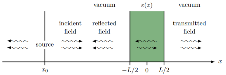
Figure 1: A one-dimensional resonator made of a homogeneous dispersive material is excited by a harmonic source located at $x_{0}$ . This interaction results in diffracted fields both in the forward (transmission) and backward (reflection) directions.

To test the validity of the derived QNMs expansion a simple one-dimensional example is shown in Fig. 1 for a homogeneous medium of thickness $L$ centered at the origin $x=0$, with a relative permittivity given by the Lorentz model $\varepsilon(z)=1-\Omega^{2}/(z^{2}-\omega_{0}^{2}+iz\gamma)$, where $\omega_{0}$ is the medium resonance frequency, $\gamma$ is the absorption parameter, and $\Omega$ is related to the electron density. This medium is surrounded by vacuum and hence acts as a Fabry-Pérot resonator.

The resonator is excited by a harmonic source of frequency $z$ located at $x_{0}$ which generates the incident electric field $E_{s}(x,z)=e^{iz|x-x_{0}|/c}{\color[rgb]{0,0,0}{e^{iz(x_{0}+L/2)/c}}}$, normalized to unity at the input interface $x=-L/2$ of the resonator. The total electric field in the whole space is given by the exact formulation [25]:

$$\begin{array}[]{rlr}E_{R}(x,z)=&{\color[rgb]{0,0,0}{E_{s}(x,z)}}+R(z)\,e^{-iz(x+L/2)/c}&x\leq{-L}/{2}\,,\\[0.0pt] E_{in}(x,z)=&A(z)\,e^{iz\sqrt{\varepsilon(z)}x/c}+B(z)\,e^{-iz\sqrt{\varepsilon(z)}x/c}&|x|\leq L/2\,,\\[0.0pt] E_{T}(x,z)=&T(z)\,e^{iz(x-L/2)/c}&x\geq L/2\,,\\[5.69054pt] \end{array}$$ (9)

where $T(z)$ and $R(z)$ are the transmission and the reflection coefficients of the dispersive resonator, and $A(z)$ and $B(z)$ can be uniquely determined by matching the fields at the two resonator interfaces. The Green’s function of the resonator can hence be analytically obtained for the case presented in Fig. 1. To begin with, the transmission function is given as [25]

$$T(z)=\frac{[1-r_{0}^{2}(z)]\,e^{iz\sqrt{\varepsilon(z)}L/c}}{1-r_{0}^{2}(z)\,e^{2iz\sqrt{\varepsilon(z)}L/c}},\quad r_{0}(z)=\frac{1-\sqrt{\varepsilon(z)}}{1+\sqrt{\varepsilon(z)}}\,.$$ (10)

It has been proven that $T(z)$ is an even function of the square root of the permittivity [21], hence it contains no branch-cut. Then, in order to use the QNMs expansion (8), the conditions (3) and (5) have to be satisfied. For the transmitted part of the field, the general derivation is applied to the function

$$G_{T}(x,z)=\frac{T(z)}{z}\>e^{iz(x-L/2)/c}\quad\quad x\geq L/2\,.$$ (11)

It can be checked that the expression (11) satisfies (3) and (5) and thus the validity of (8) is guaranteed. The set of poles $\{0,\,z_{q}:T^{-1}(z=z_{q})=0\}$ and the corresponding residues $T^{q}(z_{q})$ have been estimated and computed in Ref. [21]. The transmitted field expansion is then

$$\begin{array}[]{rl}E_{T}(x,z)=&z\displaystyle\sum_{z_{q}}\frac{T^{q}(z_{q})\,e^{iz_{q}(x-L/2)/c}}{z_{q}\,(z-z_{q})}\,e^{i(z-z_{q})(x+L/2)/c}\\[5.69054pt] +&T_{0}\,e^{iz(x+L/2)/c}\>,\end{array}$$ (12)

where $T_{0}=T(z=0)=1$. Hence it is found that the series above equals the difference $E_{T}(x,z)-e^{iz(x+L/2)/c}$ which is precisely the diffracted field in the half-space $x>L/2$. It can be noticed that the additional causality-related factor cancels the exponential growing term in the residue expression which ensures the absence of exponential growing: the terms that describe the transmitted field outside the resonator (of $x$-dependency) appear as a function oscillating at the excitation frequency $z$ only, as in [18]:

$$E_{T}(x,z)-e^{iz(x+L/2)/c}=z\sum_{z_{q}}\frac{T^{q}(z_{q})\,e^{-iz_{q}L/c}}{z_{q}\,(z-z_{q})}\,e^{iz(x+L/2)/c}.$$ (13)

Similarly, the reflection coefficient is given by [25]

$$R(z)=r_{0}(z)\,\frac{1-e^{2iz\sqrt{\varepsilon(z)}\,L/c}}{1-r_{0}^{2}(z)\,e^{2iz\sqrt{\varepsilon(z)}\,L/c}}\,.$$ (14)

The reflection coefficient $R(z)$ is also an even function of $\sqrt{\varepsilon(z)}$ and hence its spectrum is restricted to a discrete set of resonances. For the reflected part of the field, the following function is considered

$$G_{R}(x,z)=\frac{R(z)}{z}\,\,e^{-iz\,(x+L/2)/c}\,e^{-iz{\tau}}\quad\quad x\leq-L/2\,.$$ (15)

The infinitesimal time $\tau>0$ is introduced to ensure that the conditions (3) and (5) are satisfied. Therefore, the QNMs expansion (8) is valid and the reflected field expansion is

$$E_{R}(x,z)={\color[rgb]{0,0,0}{E_{s}(x,z)}}+z\sum_{z_{q}}\frac{R^{q}(z_{q})}{z_{q}\,(z-z_{q})}e^{-iz(x+L/2)/c}\,e^{i(z-z_{q})\tau}\,,$$ (16)

where the poles ${z_{q}}$ of the function $R(z)$ are the same as $T(z)$, since they share the same denominator, and $R^{q}(z_{q})$ are the residues of the function $R(z)$ at its poles. Notice that the pole at $z=0$ has no contribution since $R(0)=0$. The expression (16) shows no exponential growth for the reflected fields.

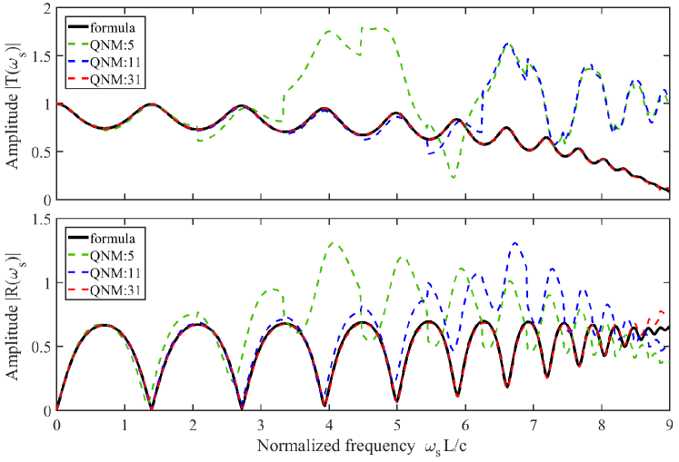
Figure 2: A comparison between the results of the exact formulas (solid lines) of $T(z)$ and $R(z)$ and their corresponding QNMs expansion (dashed lines) for below-resonance excitation $\omega_{s}<\omega_{0}$. The results are shown for different numbers of summation terms of the expansion.

Figure 2 shows the transmission function $T(z)$ and the reflection function $R(z)$ both using the exact expression (9) and the QNMs expansion (12) at $x=L/2$ for $T(z)$, and (16) at $x=-L/2$ for $R(z)$ while subtracting the incident field term. The given test case is for a Lorentz medium of parameters $\omega_{0}L/c=10$, $\gamma L/c=0.2$, and $\Omega L/c=20$, and for below-resonance excitation with unity amplitude $|E_{s}|=1$. The parameter $\tau c/L$ is set to 0.1 for the presented simulation.

The convergence analysis is also presented while the results of the exact formulation and the QNMs expansions calculations show an excellent agreement, if enough summation terms are included. As mention earlier, this parameter $\tau$ ensure the condition (5) at the expense of introducing a small error. It is possible to decrease the value of $\tau$, however, the number of modes needed to ensure the convergence is increased accordingly.

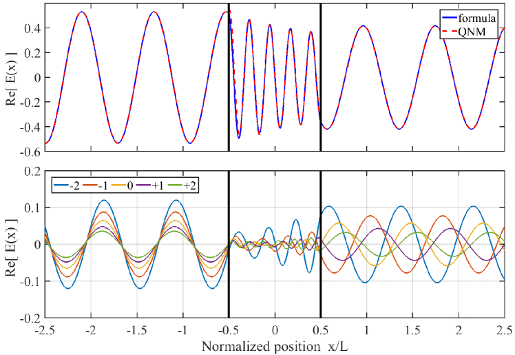
Figure 3: Top) The field distribution of a Lorentz-dispersive resonator of parameters $\omega_{0}L/c=10$, $\gamma L/c=0.2$, $\Omega L/c=20$, and for a near-resonance harmonic excitation at frequency $\omega_{s}L/c=8$. The result of the QNMs expansion using 31 modes perfectly matches the exact formula. Bottom) The field distribution of the five nearest QNMs to the excitation frequency.

The field distribution, outside as well as inside the resonator, of the given test case is presented in Fig. 3 for a near-resonance excitation at $\omega_{s}L/c=8$. The results are shown for both the exact formulation (9) and the QNMs expansion (13,16). The field inside the cavity is determined by the field continuity at the two interfaces of the resonator, i.e., the residues $A^{q}(z_{q})$ and $B^{q}(z_{q})$ are derived from $T^{q}(z_{q})$ and $R^{q}(z_{q})$ by continuity, provided that each “conventional” QNM –  before the regularization factor $e^{i(z-z_{q})|x+L/2|/c}$ is introduced by Eq. (8) –  is a mode of the Helmholtz equation. The results of the QNMs expansion perfectly match the exact formulation, with a less than $2\%$ error using $31$ QNMs, and show no divergence outside the resonator and therefore validate the proposed approach. Figure 3 also shows the field distribution of the five nearest QNMs to the excitation frequency where the mode $0$ is the central mode (the dominant mode) with the closest real frequency part to $\omega_{s}$.

Figure 4 explicitly identifies the crucial result of this manuscript. The conventional QNMs formulation is compared to the QNMs derived taken into account the causality (8). The field distribution of two QNMs from the previous example is plotted up to a large distance from the resonator. The QNMs derived using causal Green’s function show no divergence behavior, as predicted by the calculations, on the contrary to the “conventional” QNMs without the causality-related regularization factor. That finally proves that taking into account the causality principle enables the construction of well-behaved QNMs that can accurately describe the behavior of open systems.

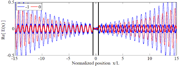
Figure 4: A comparison between the field distribution of QNMs formulation with the additional causality-related factor (solid lines) that shows no divergence outside the resonator, and the conventional QNMs formulation (dashed lines) that exhibits a divergence behavior. The results are shown for the two nearest QNMs to the excitation frequency of the example in Fig. 3.

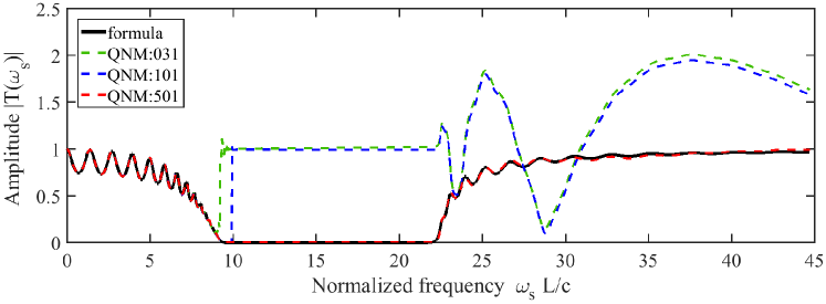
Figure 5: The exact formula for $T(z)$ and its corresponding QNMs expansion for different excitation regions. The results are shown for different numbers of summation terms in dashed lines.

It is worthy to note that the convergence is even slower for the excitation around the resonance frequency $\omega_{0}$ and above, as it can be observed for the transmission coefficient on Fig. 5. That is due to the infinite number of modes around the resonance $\omega_{0}$ [21] and to the divergence of the residues $T^{q}$ and $R^{q}$ as $\varepsilon(z){\rightarrow}1$. This divergence is then compensated by the $1/z_{q}$ factor in (12), but in this case it is needed to include many summation terms to ensure convergence.

4 Conclusion

The quasi-normal modes (QNMs) expansion of the Green’s function is derived using complex analysis and taking into consideration the frequency dispersion, the causality principle and thus the finite velocity of electromagnetic waves. The resulting formulation of the QNMs expansion shows no divergence of the fields when $|\boldsymbol{r}|\to\infty$, leading to the construction of well-behaved modes of the open system that are able to accurately describe the fields distribution inside and outside the open resonator. In this approach, the regularization process (the additional factor) is intrinsic and appears when the QNMs are redefined using the causal Green’s function formulation. A simple one-dimensional homogeneous absorptive medium with a Lorentz frequency dispersion is considered to validate the general derivation and the arguments on which it is based. The fields evaluated using the QNMs expansion, inside and outside the resonator, perfectly match the exact expressions if enough summation terms are considered. These results bring new elements to show that the QNMs can form a complete set to express in the whole space the electromagnetic fields diffracted by dispersive and absorptive materials. The general derivation is applicable to systems with a discrete set of resonances like bounded scatterers in two and three dimensions.

Funding

This work was supported by the French National Agency for Research (ANR) under the project “Resonance” (ANR-16-CE24-0013). We express our gratitude to all the participants in the project “Resonance” and to Prof. Aladin Hassan Kamel (Ain-Shams University, Egypt) for the valuable discussions.

References

- [1] S. Nie and S. R. Emory, “Probing single molecules and single nanoparticles by surface-enhanced raman scattering,” \JournalTitleScience 275, 1102–1106 (1997).
- [2] X. Huang, I. H. El-Sayed, W. Qian, and M. A. El-Sayed, “Cancer cell imaging and photothermal therapy in the near-infrared region by using gold nanorods,” \JournalTitleJournal of the American Chemical Society 128, 2115–2120 (2006).
- [3] A. Grigorenko, N. Roberts, M. Dickinson, and Y. Zhang, “Nanometric optical tweezers based on nanostructured substrates,” \JournalTitleNature Photonics 2, 365 (2008).
- [4] X. Ni, N. K. Emani, A. V. Kildishev, A. Boltasseva, and V. M. Shalaev, “Broadband light bending with plasmonic nanoantennas,” \JournalTitleScience 335, 427–427 (2012).
- [5] P. Leung, S. Liu, and K. Young, “Completeness and orthogonality of quasinormal modes in leaky optical cavities,” \JournalTitlePhysical Review A 49, 3057 (1994).
- [6] P. Leung, S. Liu, and K. Young, “Completeness and time-independent perturbation of the quasinormal modes of an absorptive and leaky cavity,” \JournalTitlePhysical Review A 49, 3982 (1994).
- [7] E. Ching, P. Leung, A. M. van den Brink, W. Suen, S. Tong, and K. Young, “Quasinormal-mode expansion for waves in open systems,” \JournalTitleReviews of Modern Physics 70, 1545 (1998).
- [8] P. T. Kristensen, C. Van Vlack, and S. Hughes, “Generalized effective mode volume for leaky optical cavities,” \JournalTitleOptics Letters 37, 1649–1651 (2012).
- [9] C. Sauvan, J.-P. Hugonin, I. Maksymov, and P. Lalanne, “Theory of the spontaneous optical emission of nanosize photonic and plasmon resonators,” \JournalTitlePhysical Review Letters 110, 237401 (2013).
- [10] R.-C. Ge, P. T. Kristensen, J. F. Young, and S. Hughes, “Quasinormal mode approach to modelling light-emission and propagation in nanoplasmonics,” \JournalTitleNew Journal of Physics 16, 113048 (2014).
- [11] R.-C. Ge and S. Hughes, “Design of an efficient single photon source from a metallic nanorod dimer: a quasi-normal mode finite-difference time-domain approach,” \JournalTitleOptics Letters 39, 4235–4238 (2014).
- [12] B. Vial, G. Demésy, F. Zolla, A. Nicolet, M. Commandré, C. Hecquet, T. Begou, S. Tisserand, S. Gautier, and V. Sauget, “Resonant metamaterial absorbers for infrared spectral filtering: quasimodal analysis, design, fabrication, and characterization,” \JournalTitleJournal of the Optical Society of America B 31, 1339–1346 (2014).
- [13] F. Alpeggiani, N. Parappurath, E. Verhagen, and L. Kuipers, “Quasinormal-mode expansion of the scattering matrix,” \JournalTitlePhysical Review X 7, 021035 (2017).
- [14] J. R. de Lasson, P. T. Kristensen, J. Mørk, and N. Gregersen, “Semianalytical quasi-normal mode theory for the local density of states in coupled photonic crystal cavity–waveguide structures,” \JournalTitleOptics Letters 40, 5790–5793 (2015).
- [15] H.-P. Nollert and B. G. Schmidt, “Quasinormal modes of schwarzschild black holes: Defined and calculated via laplace transformation,” \JournalTitlePhysical Review D 45, 2617 (1992).
- [16] D. A. Powell, “Interference between the modes of an all-dielectric meta-atom,” \JournalTitlePhysical Review Applied 7, 034006 (2017).
- [17] Q. Bai, M. Perrin, C. Sauvan, J.-P. Hugonin, and P. Lalanne, “Efficient and intuitive method for the analysis of light scattering by a resonant nanostructure,” \JournalTitleOptics Express 21, 27371–27382 (2013).
- [18] M. Kamandar Dezfouli and S. Hughes, “Regularized quasinormal modes for plasmonic resonators and open cavities,” \JournalTitlePhys. Rev. B 97, 115302 (2018).
- [19] B. Vial, F. Zolla, A. Nicolet, and M. Commandré, “Quasimodal expansion of electromagnetic fields in open two-dimensional structures,” \JournalTitlePhysical Review A 89, 023829 (2014).
- [20] P. Lalanne, W. Yan, K. Vynck, C. Sauvan, and J. Hugonin, “Light interaction with photonic and plasmonic resonances,” \JournalTitleLaser Photonics Rev. , 1700113 (2018).
- [21] M. I. Abdelrahman and B. Gralak, “Modal analysis of wave propagation in dispersive media,” \JournalTitlePhysical Review A 97, 013824 (2018).
- [22] B. Gralak, “Analytic properties of the electromagnetic green’s function,” \JournalTitleJournal of Mathematical Physics 58, 071501 (2017).
- [23] J. Makialo, M. Kauranen, and S. Suuriniemi, “Modes and resonances of plasmonic scatterers,” \JournalTitlePhys. Rev. B 89, 165429 (2014).
- [24] M. Reed and B. Simon, Methods Of Mathematical Physics. Vol. 3: Scattering Theory (Academic Press, 1979).
- [25] A. E. Siegman, Lasers (Mill Valley, CA: University Science Books, 1986).