Kardar-Parisi-Zhang Universality in First-Passage Percolation: the Role of Geodesic Degeneracy

Abstract

We have characterized the scaling behavior of the first-passage percolation (FPP) model on two types of discrete networks, the regular square lattice and the disordered Delaunay lattice, thereby addressing the effect of the underlying topology. Several distribution functions for the link-times were considered. The asymptotic behavior of the fluctuations for both the minimal arrival time and the lateral deviation of the geodesic path are in perfect agreement with the Kardar-Parisi-Zhang (KPZ) universality class regardless of the type of the link-time distribution and of the lattice topology. Pre-asymptotic behavior, on the other hand, is found to depend on the uniqueness of geodesics in absence of disorder in the local crossing times, a topological property of lattice directions that we term geodesic degeneracy. This property has important consequences on the model, as for example the well-known anisotropic growth in regular lattices. In this work we provide a framework to understand its effect as well as to characterize its extent.

I Introduction

Stochastic geometry presents a wealth of results, both from the mathematical and the physical standpoints Adler ; Itzykson_Drouffe ; Booss.book . The physics of polymers, membranes and fluctuating interfaces is described by random geometry Nelson ; Boal , as is quantum gravity in two dimensions Ambjorn_97 . Recently, it was shown that random two-dimensional Riemannian manifolds endowed with a random metric field which is a short-range perturbation of the plane metric show universal fractal properties Santalla_15 . Straight lines and circumferences, i.e. geodesics and balls, become irregular and their roughness follows scaling laws within the Kardar-Parisi-Zhang (KPZ) universality class Kardar_PRL86 which describes interfacial random growth Barabasi ; Krug_97 ; Krug_10 ; Halpin_15 . Concretely, the width of a ball with radius $R$ can be shown to scale as $W\sim R^{\beta}$, where $\beta=1/3$ is the growth exponent, and the lateral deviation of a geodesic between two points whose Euclidean distance is $L$ scales as $L^{1/z}$, where $z=3/2$ is the dynamical exponent. Moreover, the radial fluctuations at any point of a ball were shown to follow the Tracy-Widom distribution associated with the Gaussian unitary ensemble (TW-GUE) Praehofer_02 ; Takeuchi_11 ; Corwin_13 . The same calculation was performed using other base manifolds, instead of the Euclidean plane Santalla_17 . For example, for a cylinder, the KPZ class is again found, but this time the radial fluctuations follow the Gaussian orthogonal ensemble (TW-GOE).

In this work we consider the first-passage percolation (FPP) model Hammersley_65 ; Howard_04 ; Auffinger_17 , the classic discrete model of fluid flow through a random medium whose continuum counterpart is the random metric model of Refs. Santalla_15 ; Santalla_17 . The discrete representation presents a whole set of new phenomena which ask for a thorough understanding. The FPP model consists of a network in which each nearest-neighbor link is endowed with certain random crossing time. Given two nodes of the lattice, we can compute the minimal arrival time required to travel between them, and then the associated minimal-time path, i.e. the geodesic. If the link-times are allowed to fluctuate, then the arrival time will fluctuate too. Indeed, a small change in the link times may cause a large change in the minimal-time path. Thus, the statistics of minimal paths and minimal arrival times are strongly associated.

The FPP problem has been thoroughly studied on Bernoulli systems, when the link-times can only be zero or one Smythe_78 ; Ritzenberg_84 ; Kerstein_86 ; Yao_13 ; Yao_18 , and on higher dimensions Fill_93 , including random graphs and small worlds Bhamidi_10 . Indeed, the so called KPZ relation between the scaling exponents, $z(1+\beta)=2$, has been proved for FPP balls in any dimension Chatterjee_13 provided that the exponents are suitably defined Auffinger_17 . Moreover, the FPP problem bears relation to the study of directed polymers in random media (DPRM) Kardar_87 ; Krug_91 ; Halpin_95 . Results about FPP have found applications in areas as distant as magnetism Abraham_95 , wireless communications Beyme_14 , ecological competition Kordzhakia_05 or sequence alignment in molecular biology Bundschuh_00 .

We focus on an interesting property of lattice directions, not yet addressed. In the case where all link-times are equal (the so-called homogeneous or clean case), the geodesic between any pair of lattice nodes may be unique or otherwise it may be be degenerate, i.e. there is a number of different minimal-time paths connecting the two nodes all having equal (minimal) arrival times. This property, to which we will refer to as geodesic degeneracy, depends on the lattice direction, so that anisotropic behavior is expected in regular lattices. This is illustrated in Fig. 1 for the square and hexagonal lattices. In both cases points A and B are joined by a single geodesic in the homogeneous limit. Thus, that lattice direction has no geodesic degeneracy. On the contrary, there is a large number of minimal paths between A and C (only two examples have been highlighted), hence that specific lattice direction is strongly degenerate. As we will show in this paper, this property is very relevant to understand how the geodesics and the times of arrival fluctuate when the link-times are allowed to vary, specially in the pre-asymptotic regime.

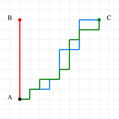
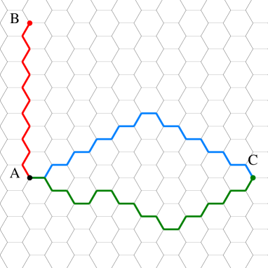
Figure 1: Illustrating the concept of geodesic degeneracy on the square (left) and hexagonal (right) lattices. We consider the homogeneous case in which link-times are equal for all links. The geodesic (minimal-time path) between points A and B is unique in both cases, while it is strongly degenerate when points A and C are considered.

We have performed a thorough numerical analysis of the arrival time statistics and geodesic geometry on two types of discrete planar lattices, a regular one given by the square lattice and a disordered Delaunay lattice formed from random points on the Euclidean plane. Delaunay lattices are triangulations which fulfill a very stringent constraint: none of the triangle circumcircles may contain any other lattice point. In addition, for a comprehensive characterization of the model we have considered several distribution functions for the link-times. Our results provide strong evidence that FPP in planar lattices falls asymptotically into the KPZ universality class. Moreover, beyond the asymptotic behavior, we were able to characterize the pre-asymptotic regime and the crossover time in both types of lattice, which may be of practical importance for specific applications of the FPP model. Note that finite simulations can well be dominated by the preasymptotic behavior, as it is common in the context of scale-invariant processes.

This article is organized as follows. Section II describes the FPP model on the square lattice, as well as the definitions employed in the article. In section III we characterize the fluctuation of the times of arrival to points along the axis and the diagonal of the square lattice, showing that the origin of their difference stems from their geodesic degeneracy. Then, in section IV we consider actual geodesics, specifically their lateral deviation, and show how the same concept allows for a complete characterization. The shapes of the growing balls for long times is the focus of Sec. V, where we address the anisotropic growth caused by the lattice anisotropy in the geodesic degeneracy. In order to distinguish the idiosincracies of the square lattice from more general features of the model, we have studied random triangulations of the plane by tracing stochastic Delaunay lattices. The results, as shown in Sec. VI, are consistent with those found for the square lattice once we consider the corresponding geodesic degeneracy. Finally, Sec. VII summarizes our conclusions and discusses interesting lines of future work.

II Model

II.1 First-passage percolation: arrival times and geodesics

Let us consider an undirected graph ${\cal L}$ with $N$ nodes and a given center node $\textbf{x}_{0}$. A link-time $t(\textbf{x}_{i},\textbf{x}_{j})$ is associated with each link between nearest-neighbor nodes $\textbf{x}_{i}$ and $\textbf{x}_{j}$. Now, we find the minimal arrival time $T(\textbf{x})$ (also referred to as passage time) from the center node $\textbf{x}_{0}$ to all other nodes on the lattice $\textbf{x}\in{\cal L}$:

$$T(\textbf{x})=\min_{m,\{\textbf{x}_{1},\cdots,\textbf{x}_{m-1}\}}\sum_{i=1}^{m}t(\textbf{x}_{i-1},\textbf{x}_{i}),$$ (1)

where we assume that $\textbf{x}_{m}=\textbf{x}$ and $t(\textbf{x},\textbf{y})=\infty$ if x and y are not nearest-neighbors. Notice that the length of the path, $m$, is also minimized. This minimal arrival time can be obtained using e.g. Dijkstra’s algorithm Cormen , which works in $O(N^{2})$ time for an arbitrary graph. Besides the minimal arrival time, Dijkstra’s algorithm also returns the parent of each node, $P(\textbf{x})$, which is the node from which x is reached when the minimal-time path is followed. Thus, by applying iteratively the parent application we eventually must reach the center node:

$$\forall\textbf{x}\in{\cal L},\quad\exists\,!n\quad|\quad P^{(n)}(\textbf{x})=\textbf{x}_{0},$$ (2)

and we call $n(\textbf{x})$ the degree of node x. Note that $n(\textbf{x})$ is the value of $m$ resulting from the minimization in Eq. (1). In this way the geodesic associated to that node (also known as optimal path) is the orbit obtained from the successive application of $P$:

$$G(\textbf{x})=\{P^{(k)}(\textbf{x}):\quad k=1,\ldots,n(\textbf{x})\},$$ (3)

It must be stressed that we have assumed that the value of $n$ is unique for each lattice node, which means that the geodesic path between lattice points is unique too. It seems to be a reasonable assumption when the distribution of the link times is continuous.

For regular lattices with constant spacing (as those illustrated in Fig. 1), the length of the geodesic path in lattice units, denoted by $l$, will be given by:

$$l(G(\textbf{x}))=n(\textbf{x}).$$ (4)

Finally, we can also define an open ball as the set of nodes which can be reached in a time smaller than a certain value $t$:

$$B(t)=\{\textbf{x}\in{\cal L}:\quad T(\textbf{x})<t\}.$$ (5)

II.2 Geometric setup and link times

The first set of results reported here were obtained in a square lattice of lateral size $2L+1$ and with $\textbf{x}_{0}$ at its geometrical center. The choice of this simple geometry obeys two purposes. From the technical point of view, it allows a large number of simulations using large lattice sizes in order to accurately characterize the asymptotic scaling of the fluctuations. Unless otherwise stated, displayed results were obtained for $L=1000$ and from $2.5\cdot 10^{4}$ simulations, which turned into $10^{5}$ points due to the $\pi/2$ rotational symmetry of the lattice.

From the fundamental point of view, the structure of the square lattice lends itself to a careful study of the effect of geodesic degeneracy, as described in the Introduction. Indeed, let us consider two nodes separated by vector $(x,y)$. In the case where all link times are equal (the so-called homogeneous case), the length of the optimal (geodesic) path between them will be $l=|x|+|y|$. However, this optimal path is typically degenerate, and the number of different geodesics connecting the two nodes is given by

$$N_{deg}(x,y)={(|x|+|y|)!\over|x|!\;|y|!},$$ (6)

which we can call the degree of degeneracy associated to the direction $(x,y)$. For a constant geodesic length, say $l=2\ell$, the highest degree of degeneracy is obtained when the sites are on a lattice diagonal ($|x|=|y|=\ell$) and it is given by $N_{deg,\text{max}}=(2\ell)!/(\ell!)^{2}\approx 2^{2\ell}$. On the other side, the lowest degeneracy corresponds to points on an axis ($\pm 2\ell,0)$ or ($0,\pm 2\ell$) resulting in $N_{deg,\text{min}}=1$, which means that the geodesic path is unique and given by the Euclidean straight line connecting the two sites. For intermediate lattice directions degeneracy increases with their angle with respect to the axis. The amount of geodesic degeneracy is an intrinsic property of the lattice, and the maximal exponential growth rate is given by the maximal eigenvalue of the associated adjacency matrix.

Most of our work will compare distances between nodes and times of arrival, so we define $d(\textbf{x}_{i},\textbf{x}_{j})$ as the standard Euclidean distance between nodes $\textbf{x}_{i}$ and $\textbf{x}_{j}$. For the square lattice we will assume that path lengths (denoted by $l$) and distances between lattices sites (given by $d$) will be given in units of the lattice spacing. It is worth noticing that times of arrival can be regarded as distances in a different metric, as it is done in Santalla_15 . Disordered lattices will be addressed in section VI and their construction will be discussed there.

Once the lattice is set, we provide each nearest-neighbor link with a crossing time $t$, which is randomly and independently chosen from a distribution function $f(t)$ with mean $\tau$ and variance $s^{2}$ (standard deviation $s$). We have worked with different distribution functions such as uniform, log-normal, Weibull, and Pareto. Let us describe briefly our choice of parameters. Uniform distributions on an interval $[t_{\text{min}},t_{\text{max}}]$ will be denoted by $\text{U}(t_{\text{min}},t_{\text{max}})$ with the following relations holding:

$$t_{\text{min}}=\tau-\sqrt{3}s,\qquad t_{\text{max}}=\tau+\sqrt{3}s.$$ (7)

We can define the amplitude of the fluctuations as $\delta_{t}\equiv t_{max}-t_{min}$ and we obtain

$$\delta_{t}=2\sqrt{3}s.$$ (8)

Log-normal distributions will be denoted as LogN$(\mu,\sigma^{2})$, where the distribution pdf is given by:

$$f(t)={1\over t\sigma\sqrt{2\pi}}\exp\left(-(\ln t-\mu)^{2}\over 2\sigma^{2}\right).$$ (9)

The Weibull distribution is denoted here by Wei$(\lambda,k)$ with pdf (only defined for positive $x$):

$$f(t)={k\over\lambda}\left({t\over\lambda}\right)^{k-1}\exp\left(-(t/\lambda)^{k}\right).$$ (10)

Finally, the Pareto distribution will be termed as Par$(t_{m},\alpha)$, defined for $t>t_{m}$, with $t_{m}$ and $\alpha>0$, and with the following pdf:

$$f(t)={\alpha t_{m}^{\alpha}\over t^{\alpha+1}}.$$ (11)

III Fluctuations of the Minimal Time of Arrival

We begin our analysis by addressing the fluctuations of the minimal time of arrival to the nodes of the square lattice as a function of the distance to the center node $\textbf{x}_{0}$, which is the origin of coordinates. Let us remark that fluctuations in the minimal arrival time correspond to the roughness of the balls Chatterjee_13 ; Santalla_15 , and will be characterized by the same scaling exponent, $\beta$, as long as it exists. Thus, within the KPZ class we expect the variance of the minimal time of arrival $\sigma^{2}_{T}\sim d^{2\beta}$, where $\beta=\frac{1}{3}$.

As discussed above, the structure of the square lattice suggests focusing the analysis on two lattice directions, the axis and the diagonal, as they stand for the limiting cases from which intermediate behavior should be readily deduced.

III.1 Scaling on the axis

We consider the times of arrival to points x on the axis, i.e. points with coordinates of the form $(\pm x,0)$ and $(0,\pm x)$, with $x=1,\ldots,L$, and whose Euclidean distance to the origin is $d(\textbf{x}_{0},\textbf{x})=x$. We show in Fig. 2 (left) the variance of the minimal time of arrival, $\sigma_{T}^{2}$, rescaled by the link-time variance $s^{2}$, as a function of the distance to the origin for different distribution functions and some representative parameters. Two different scaling regimes indicated by the broken lines are clearly observed. For most cases there is an initial regime of the form $\sigma_{T}^{2}\sim d$, which is followed by the asymptotic scaling $\sigma_{T}^{2}\sim d^{2\beta}$ with $\beta=\frac{1}{3}$, in agreement with the expected KPZ universality class Santalla_15 . The pre-asymptotic regime can be arbitrarily large and exceed the lattice limits, as in the upper curve corresponding to LogN$(0.1,0.0002)$, or arbitrarily short so that it can not be observed, e.g. lower curve, U$(0.1,9.9)$.

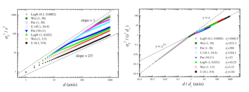
Figure 2: Fluctuations of the minimal time of arrival to points on the axis of the square lattice as a function of their Euclidean distance to the origin, for different link-time distributions. (Left) Fluctuation variance has been rescaled by the link-time variance $s^{2}$. Broken lines represent power-law behaviors with exponents 1 and 2/3, as indicated. (Right) Distance and variance have been rescaled by the corresponding crossover distance $d_{c}$, indicated for each link-time distribution in the legend. Broken lines represent the two branches of the piecewise scaling function given in Eq. (15).

The reason for the pre-asymptotic linear regime $\sigma_{T}^{2}\sim d$ is the following. As discussed above, the optimal path between two points on the axis in the uniform case $s^{2}=0$ is unique. When $s^{2}$ is positive but very small, still the geodesic will correspond to the Euclidean line because the deviation from it entails additional steps (at least two) which come at a cost in time proportional to $\tau$, the mean link-time. For short distances this is enough to preclude any deviation of the minimal-time path from the axis. In this regime the average passage time between two points separated by a distance $d$ is simply $\langle T(d)\rangle=d\tau$, and its variance comes from the straightforward addition of the link-time variances $\sigma_{T}^{2}(d)=ds^{2}$, thereby accounting for the pre-asymptotic scaling displayed in Fig. 2 (left).

The amplitude of the arrival-time fluctuations will grow with distance $d$ until it becomes large enough to assume the cost in time of an eventual deviation from the Euclidean geodesic. We will denote that critical distance by $d_{c}$. For distances above $d_{c}$ the disorder amplitude makes the underlying geometric constraint imposed by the lattice irrelevant and hence allows the geodesics to explore freely the space.

We can deduce an accurate expression for the crossover distance if we first assume Eq. (8) for the amplitude of the minimal time fluctuations $\delta_{T}(d)$,

$$\delta_{T}(d)=2\sqrt{3\sigma_{T}^{2}(d)}=2s\sqrt{3d},$$ (12)

and we note that the smallest deviation of the geodesic from the axial line necessarily entails two additional steps which, on average, represent a contribution of $2\tau$ to the passage time. After equating the amplitude of the disorder at $d_{c}$ to that cost, $\delta_{T}(d_{c})=2\tau$, we obtain

$$d_{c}={\tau^{2}\over 3s^{2}}=\frac{1}{3}\frac{1}{(\text{CV})^{2}}.$$ (13)

where CV is the coefficient of variation of the link-time distribution, defined for every $f(t)$ as the ratio of the standard deviation $s$ to the mean value $\tau$. This parameter is frequently used in statistics as a standardized measure of the dispersion of a distribution.

The expression given in Eq.(13) agrees with our qualitative description since $d_{c}$ grows with $\tau$ and decreases with $s^{2}$. Moreover, it also agrees with the results displayed in Fig. 2 (left) as it predicts a value of $d_{c}=1.04$ for case U$(0.1,9.9)$, which thus precludes the observation of the pre-asymptotic regime, and a value of $d_{c}=1666.5$ for case LogN$(0.1,0.0002)$, which indicates that the lattice size ($L=1000$) is not sufficiently large to reach the asymptotic KPZ scaling.

The validity of Eq. (13) is demonstrated in the right panel of Fig. 2, where data have been rescaled by $d_{c}$ and the curves collapse to a single universal function. That means that fluctuations of the minimal time of arrival to nodes on the axis are completely determined by the dispersion of $f(t)$, concretely by its coefficient of variation, so that different distribution functions but with the same CV will yield similar behaviors. We thus deduce the following scaling Ansatz:

$$\sigma^{2}_{T}(d)=3^{-1}\tau^{2}g\left({d\over 3^{-1}\tau^{2}s^{-2}}\right),$$ (14)

with the scaling function

$$g(x)\sim\begin{cases}x&\textrm{if }x\ll 1,\\ x^{2\beta}&\textrm{if }x\gg 1.\end{cases}$$ (15)

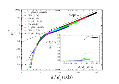
Figure 3: Variance of the geodesic length as a function of the scaled distance on the axis for the same set of results displayed in Fig. 2. The broken line indicates the linear behavior. (Inset) Corresponding average geodesic length rescaled by the Euclidean distance.

To add more consistency to our reasoning we have displayed in Fig. 3 the variance of the length of the geodesic path, $\sigma^{2}_{l}$, as a function of the rescaled distance. An excellent collapse to the following scaling function is again obtained:

$$\sigma^{2}_{l}(d)\sim q\left(d\over d_{c}\right),$$ (16)

with

$$q(x)\sim\begin{cases}0&\textrm{if }x\ll 1\\ x&\textrm{if }x\gg 1\end{cases}.$$ (17)

In the pre-asymptotic regime ($d\ll d_{c}$) optimal paths follow the Euclidean axis and $\sigma^{2}_{l}(d)=0$. Above $d_{c}$, the variance of the geodesic length increases with distance because the increase of the fluctuations allows the geodesics to explore the space, now free of geometrical constraints, in more complex ways. The distribution of the minimal-path length fluctuations approaches the normal distribution as $d$ increases so that the scaling $\sigma^{2}_{l}(d)\sim d$ seems to result from the sum of uncorrelated random variables. Details on the behavior of the average geodesic length $\langle l(d)\rangle$ (scaled by the Euclidean length $d$) are displayed in the inset of Fig. 3. As expected, for $d\ll d_{c}$ we have $\langle l(d)\rangle=d$ whereas for $d\gg d_{c}$ the ratio seems to approach a constant value that increases with the CV of $f(t)$.

III.2 Scaling on the diagonal

Let us now consider the behavior along the lattice diagonals, i.e. corresponding to points x whose coordinates are of the form $(\pm x,\pm x)$ with $x=1,\ldots,L$, and Euclidean distance to the origin given by $d(\textbf{x}_{0},\textbf{x})=\sqrt{2}x$. The growth of the variance of the minimal-time fluctuations has been displayed in Fig. 4 for the same link-time distributions considered in Fig. 2. Contrary to the axis, the pre-asymptotic regime has nearly disappeared and fluctuations start KPZ scaling (broken line) at very early times. Moreover, the small remaining transient seems to depend on the type of distribution function, being more marked for the Pareto distribution.

This is a striking result since KPZ scaling is rapidly attained even for distributions with a very small coefficient of variation (large value of $d_{c}$), e.g. LogN$(0.1,0.0002)$, for which we had obtained a trivial growth along the axis. The reason was introduced above being the degeneracy of the geodesics in the homogeneous system. When $s^{2}=0$ the minimal-time path between two points on the diagonal is degenerate. As soon as the link-time distribution is introduced on the lattice, the degeneracy is broken. However, for systems with low dispersion (CV$\ll 1$) the optimal path will be one of the geodesics of the $s^{2}=0$ case, with fixed length $l(\textbf{x})=2x$. Since degeneracy increases exponentially with the distance, at short distances the number of degenerate optimal paths will be large enough to allow the minimal arrival time to fluctuate without the geometrical constraints found along the axis direction.

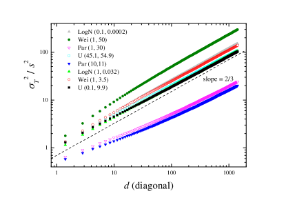
Figure 4: Scaled variance of the fluctuations of the minimal arrival time to points on the diagonal of the square lattice as a function of their Euclidean distance to the origin, for the same link-distributions considered in Fig. 2. The broken line stands for the KPZ scaling.

As expected, the effect of degeneracy is also noticeable in the behavior of the geodesic length, whose variance has been displayed in Fig. 5. Only those cases yielding non-zero fluctuations (largest values of CV) have been plotted. For distributions with low values of CV (say, $d_{c}>100$), the minimal-time path was always one of the degenerate geodesics of the homogeneous case $s^{2}=0$ so no length fluctuations were observed.

In the axis direction, KPZ scaling was directly related to the deviation of the geodesics from the Euclidean path. Along the diagonal, however, the KPZ behavior displayed in Fig. 4 has no relation to the fluctuations of the geodesic length, which show no universal features. As discussed above, the geodesic degeneracy prevents the optimal paths in the disordered case from leaving the degenerate ensemble. Only when the amplitude of the disorder is large enough to conceal the underlying lattice structure, non-negligible fluctuations of the geodesic length are observed. This happens when $d\gg d_{c}$ and becomes significant for very large values of CV. Asymptotic behavior seems to follow the same scaling as for the axis, $\sigma^{2}_{l}(d)\sim d$ (broken line in Fig. 5). The average geodesic length (scaled by the clean-case length $2x$) is displayed in the inset and shows a similar behavior, although less pronounced, to the curves displayed in the inset of Fig. 3 for the axis.

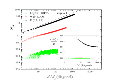
Figure 5: Variance of the geodesic length as a function of the scaled distance along the diagonal. The cases shown are the same as those displayed in Fig. 4, removing those which present zero fluctuations. The broken line indicates the linear behavior. (Inset) Corresponding average geodesic length scaled by the $l=2x$ value of case $s^{2}=0$.

III.3 Full probability distribution

The KPZ class does not only convey the scaling behavior of the passage-time fluctuations. As discussed in Santalla_15 , the full local fluctuation histogram of minimal passage times is predicted to follow the Tracy-Widom distribution for the Gaussian unitary ensemble (GUE). This prediction can be checked by measuring higher order cumulants of the time of arrival distribution, as we have done in Figs. 6 and 7 for sites on the axis and the diagonal, respectively. Left parts display the evolution of the third cumulant (skewness) with the Euclidean distance to the origin (scaled by $d_{c}$ in the case of the axis), and right panels show the results for the fourth cumulant (kurtosis). Expected TW-GUE values have been represented with horizontal broken lines.

Results are in agreement with the corresponding behaviors of the passage-time fluctuations discussed above. With regard to the axis, for distances below the crossover length geodesics are straight lines and the fluctuations in the time of arrival approach the Gaussian behavior regardless of the type of distribution. Accordingly, for $d\ll d_{c}$ the cumulants displayed in Fig. 6 approach or stay close to the Gaussian value of 0. Above $d_{c}$ a crossover of the fluctuation scaling to the KPZ class and thus of the cumulants to the TW-GUE values, takes place. With respect to the diagonal depicted in Fig. (7), the curves monotonically converge to the TW-GUE moments in agreement with the convergence to the KPZ class of the scaling of the passage-time fluctuations displayed in Fig. 4.

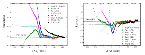
Figure 6: Skewness (left) and kurtosis (right) of the distribution of passage times to sites on the axes of the square lattice, as a function of the scaled Euclidean distance to the origin for different link-time distributions. Results for case U$(0.1,9.9)$ were obtained for $L=2000$ and from an ensemble of $1.5\cdot 10^{5}$ points. Horizontal broken lines stand for the TW-GUE values for skewness ($-0.224$) and kurtosis ($0.0934$) Santalla_15 .

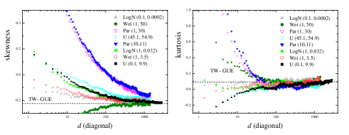
Figure 7: Skewness (left) and kurtosis (right) of the distribution of passage times to sites on the diagonal of the square lattice, as a function of the bare Euclidean distance to the origin for different link-time distributions. Results for case U$(0.1,9.9)$ were obtained for $L=2000$ and from an ensemble of $1.5\cdot 10^{5}$ points. Horizontal broken lines stand for the TW-GUE values for skewness ($-0.224$) and kurtosis ($0.0934$) Santalla_15 .

IV Geodesic Deviation

To get a complete characterization of the scaling behavior of the model we have also focused on a morphological property of the geodesics, namely, their lateral deviation. Let us define the middle point of a geodesic as the one reached in the same time from both extremes, or, in other words, the point reached at half the total passage time. The lateral deviation of the geodesic, denoted by $h$, is defined as the Euclidean distance from the middle point to the straight line joining the endpoints, as illustrated in Fig. 8.

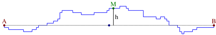
Figure 8: A sample geodesic between two points in the square lattice, $A$ and $B$, separated by 100 lattice steps. Point $M$ (marked in green) is the middle point, which can be reached from $A$ and $B$ in the same time. In blue, the middle point of the segment $\overline{AB}$, showing that both its $X$ and $Y$ components differ from those of $M$.

.

In a previous work Santalla_15 it was shown that for random metrics on 2D manifolds, the lateral deviation of the geodesic scales with the Euclidean distance $d$ between the points as $h\sim d^{1/z}$, where $z=3/2$ is the KPZ dynamical exponent. Following our line of analysis we have computed the average lateral deviation of the geodesics between the origin and points on the axis and the diagonal, and the results have been shown in Figs. 9 and 10 respectively, with the length variance $\sigma^{2}_{h}$ displayed in the insets.

In both cases the results are perfectly consistent with our findings for the fluctuations of the times of arrival. For the geodesics between points on the axis (Fig. 9) the scaling of the lateral deviation has the form:

$$h\sim b\left(d\over d_{c}\right),$$ (18)

with

$$b(x)\sim\begin{cases}0&\textrm{if }x\ll 1\\ x^{2/3}&\textrm{if }x\gg 1\end{cases}.$$ (19)

As expected, no lateral deviations are observed for $d\ll d_{c}$ and KPZ scaling is attained immediately above $d_{c}$. For the diagonal, the curves overlap showing a remarkable universal behavior which seems to be independent on the statistical properties of the local-time distribution. As for the corresponding passage-time fluctuations, convergence to the KPZ behavior is very rapid. The same analysis applies to the behavior of the length variance displayed in the insets of both figures.

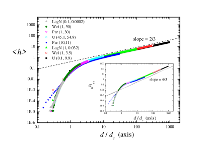
Figure 9: Average lateral geodesic deviation for points on the axis as a function of the scaled distance to the origin.(Inset) Corresponding variance of the fluctuations. KPZ scaling has been represented in both cases with the broken line.

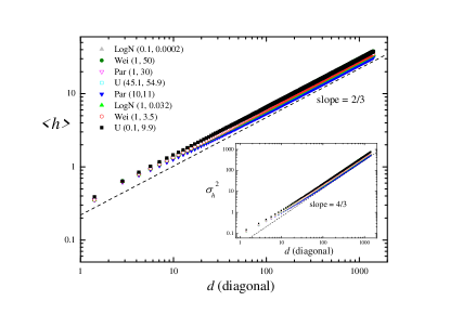
Figure 10: Average lateral geodesic deviation for points on the diagonal as a function of the distance to the origin. (Inset) Corresponding variance of the fluctuations. KPZ scaling has been represented in both cases with the broken line.

V Limit Shape

We finish the analysis of the square lattice by addressing the shape of the geodesic balls $B(t)$ defined in (5). The shape theorem Richardson_73 ; Cox-Durrett_81 ; Kesten_86 states that $t^{-1}B(t)$ converges in Hausdorff distance as $t\rightarrow\infty$ to a certain non-random, convex, compact set, with a definite shape which is expected to depend on the distribution of the passage times between neighboring lattice sites.

In order to characterize this shape we will consider the velocities of growth along the axis and the diagonal. Let $v_{A}(d)=\Delta d/\Delta\langle T\rangle(d)$ be the velocity of growth along the axis at a distance $d$, where $\langle T\rangle(d)$ is the average value of the minimal time of arrival at that position from the origin. Also, let $v_{D}(d)$ the analogous velocity for sites along the diagonal. Note that we are considering Euclidean distances, not lattice distances, hence $\Delta d=1$ along the axis and $\Delta d=\sqrt{2}$ along the diagonal, both in lattice units. We shall also consider the homogeneous case as a reference. Link-times do not vary but take the uniform value $\tau$ yielding trivially exact velocities $v_{A0}=\tau^{-1}$ and $v_{D0}=(\sqrt{2}\tau)^{-1}$, respectively.

To illustrate the behavior obtained in our model we have displayed in Figs. 11 and 12 the results of a representative link-time distribution corresponding to U$(3,4.2)$ with $d_{c}=36$. The figures display the distance $d$ of the geodesic front along the axis (Fig. 11) and the diagonal (Fig. 12) as a function of the average minimal arrival time $\langle T\rangle(d)$. Both sets of data display excellent linear behavior, so that the corresponding velocity of growth can be accurately estimated from linear regression. However, when we look at the local derivative displayed in the insets, we observe a subtle behavior not apparent in the linear plots. With regard to the growth in the axis direction (Fig. 11), for points below the crossover distance $d_{c}$ the velocity is given by the trivial one $v_{A0}$, which agrees with the fact that geodesic paths are Euclidean straight lines. A crossover takes place at $d_{c}$, beyond which the velocity increases and stabilizes at a new value which we will call $v_{A}$ (note the logarithmic scale for $d$). We can then write:

$$v_{A}(d)=\left\{\begin{array}[]{l l}v_{A0}&\mbox{for }d\ll d_{c},\\ v_{A}&\mbox{for }d\gg d_{c}.\end{array}\right.$$ (20)

Figure 11: Distance to the origin on the axis direction as a function of the average minimal arrival time to reach it. Results correspond to case U$(3,4.2)$. (Inset) Local derivative of the data in the main panel, defined as the velocity $v_{A}(d)$, as a function of distance. Horizontal broken lines indicate two regimes, $d\ll d_{c}$, with constant value $v_{A0}$, and $d\gg d_{c}$, with saturation value $v_{A}$ for the largest $d$ values.

Figure 12: Distance to the origin on the diagonal direction as as function of the average minimal arrival time to reach it. Results correspond to the U$(3,4.2)$ link-time distribution. (Inset) Local derivative of the data in the main panel, defined as the velocity $v_{D}(d)$, as a function of distance. The horizontal broken line indicates the saturation value $v_{D}$.

On the contrary, for growth along the diagonal (Fig. 12), no crossover is observed; just an initial transient is followed by saturation to a constant value denoted by $v_{D}$.

As a consequence of the minimization of the arrival time, the limit velocities $v_{A}$ and $v_{D}$ will always be larger than their uniform counterparts $v_{A0}$ and $v_{D0}$. However, this effect is more marked for degenerate directions due to the fact that geodesics do not need to leave the ensemble of degenerate paths in order to find the minimal path. We have illustrated this point in Fig. 13 for the uniform distribution with different parameter values. The limit velocities along the axis and diagonal have been rescaled by the corresponding clean values, and plotted against the CV of the distribution. In all cases the increase of the velocity is larger for the diagonal.

Another remarkable result is that these ratios are unambiguously determined by the CV, i.e. distributions with different parameter values but the same CV yield the same values for $v_{A}/v_{A0}$ and $v_{D}/v_{D0}$, so that they are undistinguishable in the figure. It should be noticed that when non-uniform distributions are used for the link-times, the results remain qualitatively only. A similar collapse to a single curve as in Fig. 13 is only obtained when the same type of distribution is used, changing its parameters. Interestingly, the two relative velocities increase with CV in a monotonic way, with $v_{A}\rightarrow v_{A0}$ and $v_{D}\rightarrow v_{D0}$ as $\mbox{CV}\rightarrow 0$. This is consistent with the fact that at this limit the distribution behaves as the Dirac delta function $\delta(t-\tau)$ and the trivial homogeneous case is recovered.

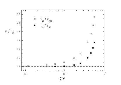
Figure 13: Ratio of the velocities of growth along the axis (solid) and diagonal (open) to their homogeneous counterparts as a function of the coefficient of variation of the different link-time distributions employed in the simulations. Note that these results correspond only to uniform link-time distributions.

It should be mentioned that the lattice size $L$ establishes a lower bound for the value of CV that allows determining the limit velocity $v_{A}$. Indeed, as shown in Eq. (20), this limit velocity is attained when $d\gg d_{c}$ or, from Eq. (13), when $d\gg 3^{-1}\mbox{CV}^{-2}$. On the other hand, all properly measured distances should be smaller than the system size, $d\ll L$. This results in $\mbox{CV}\gg(3L)^{-1/2}$, thereby establishing a lower bound for the possible values of CV that allow for a reliable measurement of $v_{A}$. For example, for $L=1000$ we have $\mbox{CV}\gg 0.018$. When $\mbox{CV}\ll(3L)^{-1/2}$ (or $d_{c}\gg L$), the velocity along the axis will then be given by $v_{A0}$. At the other extreme, the CV is bounded above by $3^{-1/2}$, which is an intrinsic property of the uniform distribution. This results in the range $[0.018,0.577]$ for the available values of CV in a lattice with $L=1000$ and uniformly distributed link times. We then define the aspect ratio $\Gamma$ of the geodesic balls as the ratio between the two limit velocities:

$$\Gamma\equiv\frac{v_{D}}{v_{A}}.$$ (21)

Results for the aspect ratio have been displayed in Fig. 14 as a function of the coefficient of variation. For those values of CV not satisfying the $\mbox{CV}\gg 0.018$ condition discussed above, we have considered $v_{A0}$ instead of $v_{A}$ (crosses in the figure). Despite being a transient regime, we see in Fig. 13 that $v_{A}\rightarrow v_{A0}$ as $\mbox{CV}\rightarrow 0$, hence we can then assume that the difference between $v_{A}$ and $v_{A0}$ is negligible when $\mbox{CV}\ll 0.018$. This approximation is validated by the continuity of the points displayed in the figure at $\textrm{CV}\approx 0.018$.

The aspect ratio of the geodesic balls is again completely determined by the coefficient of variation. As CV increases, the shape evolves from the diamond structure given by $\Gamma=(\sqrt{2})^{-1}$, attained at the limit $\mbox{CV}\rightarrow 0$ (homogeneous case), towards the circular contour given by $\Gamma=1$. These two limit shapes have been illustrated with the balls obtained at the extreme values of CV.

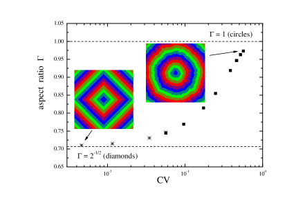
Figure 14: Aspect ratio of the geodesic balls, defined in Eq. (21), as a function of the coefficient of variation for the same results displayed in Fig. 13. Crosses stand for those values obtained after the $v_{A}=v_{A0}$ approximation. Limiting cases have been indicated with horizontal broken lines. Illustrations depict the growth of the balls $B(t)$ in a $401\times 401$ lattice for the two extreme cases for the link-time distribution: (left) U$(4.96,5.04)$ with color changing after $\Delta t=125$; (right) U$(0.1,9.9)$ with $\Delta t=60$.

VI Delaunay Lattices

The previous sections have discussed the FPP model on a square lattice. In such regular systems it is quite straightforward to recognize both unique and degenerate directions, as illustrated in Fig. 1. Also, it is rather easy to calculate the exact geodesic degeneracy for each lattice direction, as we did in Eq. (6) for the square lattice. It is therefore very pertinent to ask whether non-regular lattices might lead to different behavior. It seems reasonable to think that disordered lattices in general will present a certain degree of geodesic degeneracy that, contrary to ordered lattices, will be isotropic and dependent only on distance between the nodes. This degeneracy will increase with $d$ and will be subject to some fluctuations.

In this section we consider the FPP model on disordered planar lattices built as Delaunay lattices. A Delaunay lattice is a triangulation which fulfills a certain optimality condition: the circumscribed circle built on any triangle does not contain any other lattice points. Given a set of $N$ points on the plane, the Bowyer-Watson algorithm Bowyer_81 ; Watson_81 builds a Delaunay lattice in $O(N\log(N))$ steps in average, or $O(N^{2})$ in the worst cases Rebay_93 .

The geometric setup is as follows. We consider the unit circle with the central node $\textbf{x}_{0}$ at its geometrical center. Then we mark a set of $N_{m}$ points at fixed distances from the center, where measurements will take place. To avoid unwanted correlations, measurement points are homogeneously distributed on a spiral so that the coordinates of the $j$-th point $\textbf{x}_{j}$ ($j=1,\dots,N_{m}$) are $x_{j}=j/N_{m}\sin(j2\pi\varphi)$ and $y_{j}=j/N_{m}\cos(j2\pi\varphi)$, where $\varphi$ is the golden ratio. Accordingly, the Euclidean distance of these points to the origin is $d(\textbf{x}_{j})=j/N_{m}$. Next, we choose other $N-N_{m}$ uniformly distributed random points on the circle and we build the Delaunay lattice of the whole set of points (see Fig. 15 for an example). Notice that the lengths of the resulting links can vary notably. As for the square lattice, we associate to each link a crossing time, which is randomly chosen from a given probability distribution, hence disregarding the actual length of the link. Finally, we obtain the minimal traveling time from the origin to all lattice points.

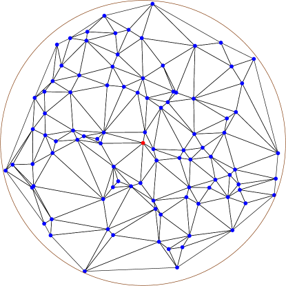
Figure 15: Example of Delaunay lattice built on $N=100$ points randomly distributed on the unit circle. The point marked in red is at the center.

Each simulation of the system corresponds to a different realization of the link time distribution, always using the same fixed lattice. It must be stressed that simulations of Delaunay lattices are more demanding computationally than for the square lattice, so the ensemble of realizations performed here is markedly less significant. Besides, since qualitative behavior does not depend on the link-time distribution function, for simplicity we will only consider the uniform distribution. The presentation of the results will follow the same scheme as used for the square lattice.

We start by showing in Figure 16 the fluctuations in the minimal arrival time as a function of the distance to the center. As in Fig. 2 (right), the variance of the passage time has been expressed in units of $s^{2}d_{c}$, while the Euclidean distance to the center, $d$, has been firstly scaled in terms of lattice jumps by a certain characteristic lattice length $a_{0}$, and then rescaled by the crossover distance $d_{c}$. Different values for $a_{0}$ have been employed, all leading to very similar results. Hereafter we will consider that the characteristic length $a_{0}$ is given by the mean link length obtained from the link length distribution, which for the fixed lattice employed here ($N=10^{5}$) was $0.0064$ with a standard deviation of $0.0033$. However, results do not change significantly if we consider the average geometric distance between nodes calculated as $\sqrt{\pi/N}$ (equal to $0.0056$ for $N=10^{5}$), or whether, instead of $d/a_{0}$, we consider the exact number of links included in the minimal path of the homogeneous case $s^{2}=0$, which we will denote by $n_{H}(d)$.

Results shown in Fig. 16 for the Delaunay lattice are quite similar to those displayed in Fig. 2 for the axis direction on the square lattice. A fairly good collapse to the scaling function given in Eq. (15) is observed. This result allows us to claim that the effective geodesic degeneracy in the Delaunay lattice is rather weak, although it is not exactly null as it was along the axis on the square lattice. Indeed, as we illustrate in Fig. 17, the minimal path between two nodes in the homogeneous case may experience local bifurcations without this entailing additional links. This contributes to the geodesic degeneracy in terms of $N_{deg}$ (which also increases exponentially) but has little impact on the results because the degree of overlap among the degenerate geodesics is very significant (notice that there are many links which are shared by all the paths), contrary to what happens along the diagonal direction on the square lattice, for instance. This behavior highlights the need to refine our definition of geodesic degeneracy, which so far has been based on the number $N_{deg}$ of degenerate paths. Although it can be considered as a first approximation, it clearly does not convey any information on the overlap among the different paths, which is certainly relevant and will be a matter of ongoing work.

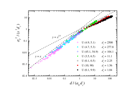
Figure 16: Scaled variance of the arrival time as a function of the Euclidean distance to the center, scaled with the mean link length $a_{0}$ and $d_{c}$, in the Delaunay lattice for different parameters of the uniform link-time distribution. Results were obtained from $1000$ simulations and $N=10^{5}$. Broken lines indicate the two branches of the scaling function given in Eq. (15).

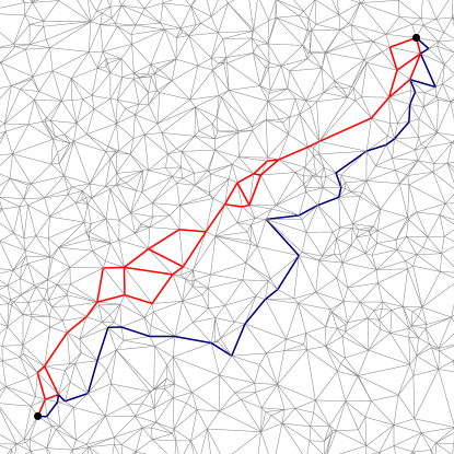
Figure 17: Geodesic degeneracy in Delaunay lattices. Red color highlights the ensemble of minimal paths obtained in the homogeneous $s^{2}=0$ case between the two lattice nodes identified by the thick points. We have $n_{H}=23$. Dark blue color identifies a geodesic path obtained in a given realization of the case U(0.5,2), which is made up of $n=33$ links.

The consequences of the weak geodesic degeneracy in Delaunay lattices are also reflected in the geometrical properties of the minimal path such as the geodesic length $l$. In the square lattice this length was uniquely determined by the number $n$ of links that make up the geodesic path, see Eq. (4). For disordered lattices, however, there is a distribution of link lengths so that these two magnitudes must be considered separately. Figure 18 displays the variance of the number of steps involved in the minimal path, $\sigma^{2}_{n}$, as a function of the rescaled distance. The inset shows the expected value of that magnitude, $\langle n\rangle$, divided by the value obtained for $s^{2}=0$, $n_{H}$. Fig. 19 shows corresponding results for the actual geodesic length, $l$, which hence takes into account actual link lengths. In the main part we display the length variance, $\sigma_{l}^{2}$, corrected by subtracting the length variance of the homogeneous $s^{2}=0$ case, denoted as $\sigma_{l,H}^{2}$, which can be viewed as a sort of intrinsic variance associated to the lattice disorder. In the inset we show the average geodesic length, $\langle l\rangle$, divided by the same magnitude in the $s^{2}=0$ case, denoted by $\langle l_{H}\rangle$.

We must first note the similarity between both plots despite the fact that the actual length involves geometrical aspects of the lattice not considered in the number of links. Both Figures 18 and 19 show a reasonably good data collapse, similar to that found in Fig. 3 for the geodesic length along the axis direction in the square lattice, adding consistency to our claims. There, the geodesic for the clean case was unique and trivial. Here, the degeneracy of the minimal path in the clean case contributes with an intrinsic dispersion that must be corrected in the raw data to recover the expected behavior. Note also the large fluctuations obtained when $d/(a_{0}d_{c})<1$, which are a consequence of the intrinsic disorder in the lattice topology. For Delaunay lattices, the cost of a deviation from the geodesic of the homogeneous case is smaller than for the axis on the square lattice. Besides, the remaining geodesic degeneracy for $s^{2}=0$ also favors deviations by enlarging the space of possible optimal paths. Therefore, the expected fluctuations for $d/a_{0}<d_{c}$ are larger than on the square lattice, justifying the scattered data for low values of $d$ in both figures.

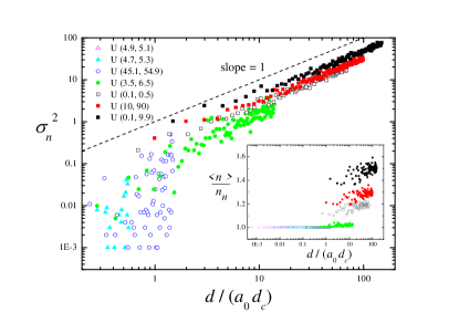
Figure 18: Variance of the number of links of the minimal path as a function of the scaled distance in the Delaunay lattice for the same set of link-time distributions displayed in Fig. 16. The broken line indicates the expected linear behavior. (Inset) Corresponding average number of links in the geodesic path divided by the number of links in the minimal path of the homogeneous $s^{2}=0$ case, $n_{H}$.

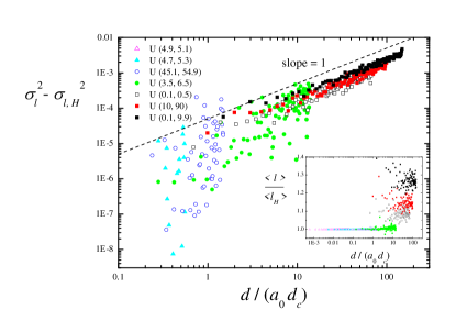
Figure 19: Variance of the length of the minimal path, corrected by the variance of the geodesic length in the homogeneous $s^{2}=0$ case, as a function of the scaled distance in the Delaunay lattice for the same set of results displayed in Fig. 16. The broken line indicates the expected linear behavior. (Inset) Corresponding average path length divided by its homogeneous counterpart, $\langle l_{H}\rangle$.

We finally address the lateral deviation of the geodesics in Delaunay lattices. As discussed in Sec. IV, the lateral deviation was defined as the Euclidean distance from the half-time point of the geodesic to the straight line joining the end nodes. For the square lattice no further distinction was necessary inasmuch as that line had a clear physical meaning: in the case of the axis direction it accounted for the geodesic path of the homogeneous system, while for the diagonal direction it represents the average path of the ensemble of degenerate geodesics. In Delaunay lattices, however, the average geodesic path of the clean case is no longer a straight line (see Fig. 17) but an intricate curve to which we can associate a mean lateral deviation $\langle h_{H}(d)\rangle$ obtained from the average of the lateral distance of the degenerate (or not) middle point. Note that we are considering absolute values for $h$. Following our line of argumentation, we must correct the raw average value obtained from different realizations of the link-time distribution, $\langle h(d)\rangle$, by subtracting the average deviation of the clean case. The behavior of the resulting corrected lateral deviation $|\langle h(d)\rangle-\langle h_{H}(d)\rangle|$ has been displayed in Fig. 20. We must point out that preliminary results obtained at the fixed measurement points were rather noisy, so we have performed an average of this quantity over all lattice points at distance $(d,d+dr)$. We can readily recognize in Fig. 17 the behavior displayed in Fig. 9 for the axis direction in the square lattice.

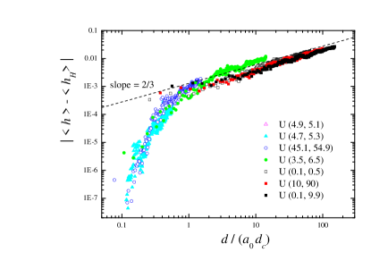
Figure 20: Average lateral deviation corrected by the value of the homogeneous case as a function of the scaled distance in the Delaunay lattice. KPZ scaling has been represented with the broken line. Results for a given distance $d$ were obtained from the average over all lattice nodes in a circular ring centered at the origin with radius $d$ and thickness $dr=1/300$.

.

Our claim that the geodesics in a fixed Delaunay lattice present low degeneracy receives further support from a probabilistic argument. Let $P(h)$ be the probability density function for the lateral deviation of all geodesics joining two fixed points. For strong disorder in the link-times, the geodesics ensemble form a wide cloud and the distribution $P(h)$ is very broad. In the homogeneous limit, the distribution must be narrower. Yet, the variance is sometimes high because the geodesic ensemble reduces to a few curves which can be very distant. Thus, $P(h)$ in the homogeneous limit is conformed by a sum of delta peaks, and the variance is not a good measure of its concentration. A better observable is given by the entropy of the distribution Vasicek.76 , specifically the Kullback-Leibler divergence Desurvire_09 which quantifies the relative entropy with respect to a homogeneous probability distribution on a fixed interval note_entropy .

Figure 21 depicts such an average relative entropy of $P(h)$ for the geodesic ensembles previously analysed, as a function of the Euclidean distance between the extreme points in units of $(a_{0}d_{c})$. For very low $d/(a_{0}d_{c})$ the entropy approaches a fixed value, related to the expected number of different geodesic paths in the homogeneous Delaunay lattice. For $d/(a_{0}d_{c})\gg 1$, the collapse of the curves is remarkable; the entropy grows logarithmically with the distance, making the curve appear as a straight line due to the logarithmic scale chosen for the horizontal axis. Since the relative entropy of a Gaussian distribution with variance $\sigma^{2}$ is proportional to $\log(\sigma^{2})$, we may conjecture that the entropy of $P(h)$ for large $d/(a_{0}d_{c})$ should behave like $(2/z)\log(d)$. Indeed, as displayed in the figure, the slope of the curves approaches $4/3$ for large $d/(a_{0}d_{c})$.

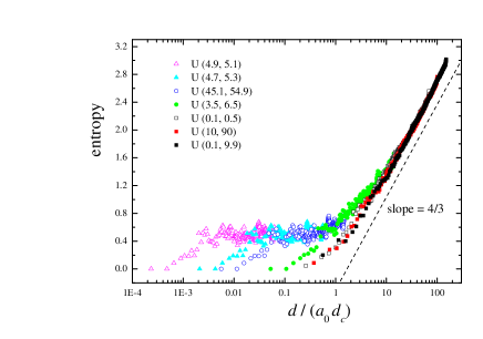
Figure 21: Relative entropy of the probability density function for lateral deviations of the geodesic ensemble as a function of the rescaled Euclidean distance in the Delaunay lattice for the same system displayed in Fig. 20. Notice the logarithmic scale on the horizontal axis.

VII Conclusions and Further work

In this work we have elucidated the role of what we have termed geodesic degeneracy, an intrinsic property of the lattice connectivity, on the scaling behavior of the first-passage percolation model in discrete planar lattices. We have considered both regular and disordered lattices, using as examples the square lattice and Delaunay lattices over uniformly scattered random points.

With regard to the asymptotic scaling behavior, a thorough analysis of both regular and disordered systems clearly support the conjecture (not yet proved rigorously) that the FPP model belongs to the KPZ universality class. Our study covers the fluctuations in the times of arrival, the geodesic lengths and their lateral deviations, explicitly demonstrating universal behavior with respect to the type of lattice and crossing-time distribution functions.

On the other hand, the pre-asymptotic behavior strongly depends on the geodesic degeneracy of the lattice direction of growth. When the geodesic in the homogeneous limit is unique or weakly degenerate, a pre-asymptotic trivial scaling corresponding to the linear growth along that direction is obtained. In this regime, the geodesic path follows the minimal path of the clean case until arrival time fluctuations are sufficiently strong to break that geometrical constraint. At this point the minimal path initiates a strongly fluctuating behavior that follows the expected KPZ scaling. On the contrary, if the minimal path is strongly degenerate in the homogeneous case, the geodesic path does not have such topological constraints and is free to fluctuate from the very beginning. Then KPZ scaling is rapidly approached. Although some heuristic arguments to characterize the degree of the geodesic degeneracy were provided, we are aware that a formal definition remains to be provided.

Interestingly, the crossover from linear growth to KPZ scaling along weakly degenerate directions seems to be uniquely determined by the coefficient of variation (CV) of the link-time distribution, regardless of the ordered or disordered nature of the underlying lattice. The crossover length and thus the extent of the pre-asymptotic regime is inversely proportional to the squared dispersion of the link-times: $d_{c}\sim\mbox{CV}^{-2}$.

The dependence of the geodesic degeneracy on the lattice direction leads to anisotropic growth on regular lattices, where an angular dependence of the degree of geodesic degeneracy occurs. This anisotropy is reflected in the kinetics and shape of the growing geodesic balls. Stronger disorder in the link-time distribution unavoidably entails faster growth than in the homogeneous case. However, this effect is favored by the degeneracy of the lattice direction. Again, the coefficient of variation emerges as a key parameter by determining the velocity of growth along the different lattice directions and hence the asymptotic shape of the geodesic ball. For irregular lattices with isotropic disorder we can accordingly expect isotropic growth.

The preasymptotic regime of FPP ($d\ll d_{c}$) for a strongly degenerate direction bears a strong similarity to a directed polymer in a random medium (DPRM) at zero temperature Kardar_87 ; Krug_91 ; Halpin_95 , if the rightwards and upwards links attached to any site are forced to be equal. Indeed, the allowed directed polymer configuration coincides with what we called degenerate paths. Nonetheless, for $d>d_{c}$, the geodesic can fold back, and the set of allowed geodesics becomes much larger than the set of allowed directed polymer configurations. Interestingly, both of them will be ruled by the KPZ class.

We should end by stressing that we have dealt only with distributions with $\mbox{CV}<1$ ($d_{c}>1$). For distributions with a stronger dispersion the pre-asymptotic behavior is not observed and different interesting effects arise which deserve additional investigation and remained beyond the scope of the present work.

- (1) R. Adler and J. Taylor, Random fields and geometry, Springer (2007).
- (2) C. Itzykson and J.-M. Drouffe, Statistical Field Theory, Cambridge University Press (1991).
- (3) B. Booß-Bavnbek, G. Esposito and M. Lesch, New paths towards quantum gravity, Springer (2009).
- (4) D. Nelson, T. Piran and S. Weinberg, Statistical Mechanics of Membranes and Surfaces World Scientific, Singapore (2004).
- (5) D. H. Boal, Mechanics of the cell, Cambridge University Press (2012).
- (6) J. Ambjørn, B. Durhuus and T. Jonsson, Quantum Geometry: A Statistical Field Theory Approach, Cambridge University Press (1997).
- (7) S.N. Santalla, J. Rodriguez-Laguna, T. LaGatta, R. Cuerno, New J. Phys. 17 033018 (2015).
- (8) M. Kardar, G. Parisi, Y.-C. Zhang, Phys. Rev. Lett. 56, 889 (1986).
- (9) A.-L. Barabási and H. E. Stanley, Fractal Concepts in Surface Growth, Cambridge University Press (1995).
- (10) J. Krug, Adv. Phys. 46, 139 (1997).
- (11) T. Kriecherbauer, J. Krug, J. Phys. A: Math. Theor. 43, 403001 (2010).
- (12) T. Halpin-Healy, K. Takeuchi, J. Stat. Phys. 160, 794 (2015).
- (13) K. A. Takeuchi, M. Sano, T. Sasamoto, H. Spohn, Sci. Rep. 1, 34 (2011).
- (14) M. Prähofer, H. Spohn, J. Stat. Phys. 108, 1071 (2002).
- (15) I. Corwin, J. Quastel, D. Ramenik, Comm. Math. Phys. 317, 347 (2013).
- (16) S.N. Santalla, J. Rodriguez-Laguna, A. Celi, R. Cuerno, J. Stat. Mech. 023201 (2017).
- (17) J. M. Hammersley and D. J. A. Welsh, “First-passage percolation, subadditive processes, stochastic networks and generalized renewal theory”, in Bernoulli, Bayes, Laplace anniversary volume, J. Neyman and L. M. LeCam eds., Springer-Verlag (1965), p. 61.
- (18) C. D. Howard, “Models of first passage percolation”, in Probability on discrete structures, H. Kesten ed., Springer (2004), p. 125–173.
- (19) A. Auffinger, M. Damron, J. Hanson, 50 years of FPP, University Lecture Series 68, American Mathematical Society (2017).
- (20) R.T. Smythe, J.C. Wierman, First-passage percolation on the square lattice, Springer Verlag (1978).
- (21) A.L. Ritzenberg, R.J. Cohen, Phys. Rev. B 30, 4038 (1984).
- (22) A.R. Kerstein, B.F. Edwards, Phys. Rev. B 33 3353 (1986).
- (23) C.-L. Yao, Stat. & Prob. Lett. 83, 797 (2013).
- (24) C.-L. Yao, Stoch. Proc. Appl. 128, 445 (2018).
- (25) J.A. Fill, R. Pemantle, Ann. Appl. Probab. 3, 593 (1993)
- (26) S. Bhamidi, R. van der Hofstad, G. Hooghiemstra, Ann. Appl. Probab. 20, 1907 (2010).
- (27) S. Chatterjee, Ann. Math. 177, 663 (2013).
- (28) M. Kardar, Y.-C. Zhang, Phys. Rev. Lett. 58, 2087 (1987).
- (29) J. Krug, H. Spohn, in Solids far from equilibrium, Ed. C. Godrèche, Cambridge University Press (1991).
- (30) T. Halpin-Healy, Y.-C. Zhang, Phys. Rep. 254, 215 (1995).
- (31) D.B. Abraham, L. Fontes, C.W. Newman, M.S.T. Piza, Phys. Rev. E 52, R1257 (1995).
- (32) S. Beyme, C. Leung, Ad Hoc Netw. 17, 60 (2014).
- (33) G. Kordzakhia, S.P. Lalley, Stoch. Proc. App. 115, 781 (2005).
- (34) R. Bundschuh, T. Hwa, Discr. Appl. Math. 104, 113 (2000).
- (35) T.H. Cormen, C.E. Leiserson, R.L. Rivest, C. Stein, Introduction to algorithms, The MIT Press (1990).
- (36) D. Richardson, Proc. Cambridge Phil. Soc. 74, 515 (1973).
- (37) J. T. Cox, R. Durrett, Ann. Probab. 9, 583 (1981).
- (38) H. Kesten, “Aspects of First-Passage Percolation” in Lect. Notes in Mathematics 1180, 125-264. Springer Verlag (1986).
- (39) A. Bowyer, Comput. J. 24, 162 (1981).
- (40) D.F. Watson, Comput. J. 24, 167 (1981).
- (41) S. Rebay, J. Comp. Phys. 106, 127 (1993).
- (42) O. Vasicek, J. Roy. Statist. Soc. Ser. B 38, 54 (1976).
- (43) E. Desurvire, Classical and quantum information theory, Cambridge University Press (2009).
- (44) We should emphasize that we do not measure the differential entropy, because it is not invariant under reparametrizations. Instead, we obtain the relative entropy, also called Kullback-Leibler divergence Desurvire_09 , with respect to a homogeneous probability distribution in a fixed interval. The same reference distribution should be used for all measurements in order to be compared.