Material Scaling and Frequency-Selective Enhancement of Near-Field Radiative Heat Transfer for Lossy Metals in Two Dimensions via Inverse Design

Abstract

The super-Planckian features of radiative heat transfer in the near-field are known to depend strongly on both material and geometric design properties. However, the relative importance and interplay of these two facets, and the degree to which they can be used to ultimately control energy flow, remains an open question. Recently derived bounds suggest that enhancements as large as $|\chi|^{4}\lambda^{2}/\left(\left(4\pi\right)^{2}\text{Im}\left[\chi\right]^{2}d^{2}\right)$ are possible between extended structures (compared to blackbody); but neither geometries reaching this bound, nor designs revealing the predicted material ($\chi$) scaling, have been previously reported. Here, exploiting inverse techniques, in combination with fast computational approaches enabled by the low-rank properties of elliptic operators for disjoint bodies, we investigate this relation between material and geometry on an enlarged space structures. Crucially, we find that the material proportionality given above does indeed emerge in realistic structures. In reaching this result, we also show that (in two dimensions) lossy metals such as tungsten, typically considered to be poor candidate materials for strongly enhancing heat transfer in the near infrared, can be structured to selectively realize flux rates that come within $50\%$ of those exhibited by an ideal pair of resonant lossless metals for separations as small as $2\%$ of a tunable design wavelength.

Radiative heat transfer (RHT) between objects separated by near-field distances (on the order or shorter than the thermal wavelength) exhibits a number of remarkable features. Primarily, evanescent contributions, absent in the far-field, cause the rate of heat exchange to scale inversely with separation down to nanometer scales, leading to flux rates many orders of magnitude larger than those predicted by the Stefan–Boltzmann (blackbody) law Kittel et al. (2005); Kim et al. (2015); Song et al. (2015); St-Gelais et al. (2016). Further, this increased flux can be enhanced and controlled by resonant electromagnetic surface modes Pendry (1999); Carminati and Greffet (1999); Volokitin and Persson (2001); Babuty et al. (2013), allowing heat to be concentrated into narrow and designable spectral bandwidths. These properties, in principle, provide a means of significantly improving the degree to which heat can be manipulated compared to thermal conduction, leading to the consideration of applications and devices based on near-field RHT in various contexts, with proposals ranging from thermophotovoltaics energy capture Narayanaswamy and Chen (2003); Laroche et al. (2006); Park et al. (2008); Ilic et al. (2012); Karalis and Joannopoulos (2017); St-Gelais et al. (2017) to high-density heat management Guha et al. (2012); Yang et al. (2013); Khandekar et al. (2018), and heat assisted magnetic recording Challener et al. (2009); Bhargava and Yablonovitch (2015).

Yet, a concrete understanding of what can be accomplished with near-field RHT remains elusive. Simple high-symmetry structures where analytic solutions are possible provide valuable insight, but appear to be far from ideal. In particular, the most well-studied platform for implementing selective RHT enhancement Volokitin and Persson (2007); Iizuka and Fan (2015), involving parallel metal plates Domoto et al. (1970); Kralik et al. (2012); Ijiro and Yamada (2015); Lang et al. (2017) supporting surface resonances (plasmon or phonon polaritons) Shen et al. (2009); Luo and Chen (2013), has critical deficiencies. First, as dictated by the Planck distribution, there is a natural wavelength scale for observing significant thermal radiative effects near ambient temperatures that spans the near to mid infrared (1 to $10\;\mu$m) spectrum Basu et al. (2007); Rephaeli and Fan (2009); Molesky et al. (2013). Typical (low-loss) optical materials do not support polariton resonances at these wavelengths, and often lack sufficient thermal stability to withstand longterm operation Nagpal et al. (2011); Rinnerbauer et al. (2013); Dyachenko et al. (2016). Second, the tightest known limits of RHT between extended structures, recently derived using energy conservation and reciprocity arguments Miller et al. (2015), reveal that both practical material ($|\chi|^{2}/\text{Im}\,\chi$) and geometric ($\lambda/d$) factors seemingly enable enhancements relative to blackbody emission as large as

$$\mathcal{F}_{\mathrm{limit}}\leq\left(\frac{1}{4\pi}\frac{\lambda}{d}\frac{|\chi|^{2}}{\text{Im}[\chi]}\right)^{2},$$ (1)

orders of magnitude larger than what is achievable with ideal planar media, suggesting that dramatic improvements are possible through the use of nanostructured surfaces Miller et al. (2015). (In this expression, $d$ stands for separation, and $\chi$ material susceptibility, assumed to be the same in both bodies.) Moreover, the $|\chi|^{4}/\text{Im}\left[\chi\right]^{2}$ scaling in (1) indicates that materials exhibiting strong metallic response, far from the typical planar surface–plasmon polariton (SPP) condition $\text{Re}\left[\chi\right]=-2$, have much greater potential for enhancement. To date, however, this behaviour has not been observed, and tested geometries employing non-resonant materials Fernández-Hurtado et al. (2017); Dai et al. (2017); Guérout et al. (2012); Lussange et al. (2012); Liu and Shen (2013) have yet to surpass the optimal rates associated with planar bodies.

In this article, we provide direct evidence of this material scaling enhancement in periodic systems. Building on our earlier examination of RHT between multilayer bodies Jin et al. (2017), we now employ inverse design Molesky et al. (2018) to investigate RHT between generalized two-dimensional gratings (restricting the analysis to realistic materials and fabricable structures). Focusing on lossy metals far from the SPP condition at infrared wavelengths, we observe that while $\mathcal{F}$ does not approach (1), the predicted material scaling is nevertheless present. For the specific example of tungsten (W), we also find a grating geometry that selectively achieves $50\%$ of the RHT of a pair of ideal, lossless metal plates satisfying the SPP condition, for separations as small as $2\%$ of a tunable design wavelength. These predictions represent RHT enhancements of nearly two orders of magnitude compared to corresponding planar objects, confirming the potential of even relatively simple structuring for selectively enhancing RHT.

The application of inverse design to selective RHT enhancement between extended structures is complicated in several ways. First, near-field RHT is controlled by evanescent electromagnetic fluctuations. The large density of these states makes it challenging to apply traditional resonant nanophotonic strategies for enhancing far-field emission over narrow spectral windows Pralle et al. (2002); De Zoysa et al. (2012). Moreover, the characteristically large field amplitudes and sub-wavelength features of evanescent states make them sensitive to small variations in structural and material properties Liu et al. (2010), and correspondingly accurate modeling of RHT requires fine numerical resolution Rodriguez et al. (2011, 2012); Otey et al. (2014); Messina et al. (2017).) Second, unlike the far field, RHT can not be decomposed into approximately equivalent independent subproblems. Alterations in the structure of any one object affects the response of the entire system, meaning that the scattering properties of all bodies must be controlled simultaneously. Finally, Maxwell’s equations depend nonlinearly on the dielectric properties and shapes of all bodies, making the optimization non-convex Boyd and Vandenberghe (2004) and any a priori guarantee of globally optimal solutions impossible.

Consequently, tractable general approaches for simply calculating near-field RHT have only recently been realized Rodriguez et al. (2011, 2012); Otey et al. (2014); Edalatpour and Francoeur (2016), and nearly all previously studied geometries have been designed via trial-and-error approaches exploiting brute-force search over a handful of high-symmetry design parameters Liu et al. (2015a). Beginning with bulk metamaterials Biehs et al. (2011); Guo et al. (2012); Liu and Shen (2013); Liu et al. (2013, 2014); Shi et al. (2015); Didari and Mengüç (2015), thin films Ben-Abdallah et al. (2009); Francoeur et al. (2010); Basu and Francoeur (2011); Van Zwol et al. (2011); Pendharker et al. (2017), plasmonic materials Naik et al. (2013); Pendharker et al. (2017); Liu et al. (2014); Edalatpour and Francoeur (2016); Chalabi et al. (2016), and more recently, metallic metasurfaces Liu and Zhang (2015); Fernández-Hurtado et al. (2017); Zheng et al. (2018) and gratings Lussange et al. (2012); Liu and Zhang (2014); Dai et al. (2015); Liu et al. (2015b); Chalabi et al. (2016), selective RHT enhancement has primarily been achieved by tuning the permittivity response, either real or effective, to create or mimic surface resonances . (Notably, a recent silicon metasurface design Fernández-Hurtado et al. (2017) was predicted to have a larger integrated RHT than planar SiO₂, which exhibits low-loss surface phonon polaritons, down to gap distances of $10\;\text{nm}$.) Other similarly high symmetry approaches have sought to increase the photonic density of states by exploiting interference (hybridization Prodan et al. (2003)) among the localized plasmons of individual nanostrutures Biehs et al. (2010). Building from simple shapes, tunable RHT rates have been demonstrated in nanobeam (triangluar, ellipsoidal, and rectangular unit cells) and nanoantenna arrays exploiting both Mie Chalabi et al. (2015) and Fano Baldwin et al. (2014); Pérez-Rodríguez et al. (2017) resonances. Although conceptually promising, these approaches have been found to have diminishing returns at small separations (relative to the thermal wavelength).

In the case of periodic gratings, RHT is

$$\Phi(\omega)=\frac{1}{2\pi}\int\frac{\mathrm{d}^{n}\mathbf{k}}{(2\pi)^{n}}\;\mathcal{T}\left(\omega,\textbf{k}\right),$$ (2)

where the integration is carried out over Bloch-vectors $\mathbf{k}$ in the first Brillouin zone (BZ), and the scattering properties of the structures are captured by the transfer function $\mathcal{T}\left(\omega,\textbf{k}\right)$ described by (6). To maximize the transfer function, both the density and coupling efficiency of the participating states Molesky and Jacob (2015); Liu et al. (2017) must be made as large as possible at all k. A similar problem arises in the design of far-field emitters Wang and Menon (2013); Ganapati et al. (2014); Diem et al. (2009); Liu et al. (2010); Hedayati et al. (2011); Nguyen et al. (2017), where resonant structures are often intuitively designed to match the absorption and coupling rates of a wide range of externally excited states, leading to a complete suppression of scattered fields. But the task here is more complicated, as the electromagnetic field must be regulated over a much larger (evanescently coupled) range. For intuition based structures with a few tunable parameters, there does not seem to be enough design freedom to reach this level of control, with the range of rate-matched states occurring in current designs Dai et al. (2017) falling short of those achievable in planar high index dielectrics ($n>3$). Without a viable means of addressing these questions, we turn to inverse techniques Molesky et al. (2018).

As an initial step towards the broader development of this area, and for computational convenience, we focus exclusively on two-dimensional gratings. This choice has major consequences for the underlying physical processes. Particularly, in moving from three to two dimensions, the geometric and material scaling of the density of states decreases and as a result, the maximum RHT rate between two ideal planar metals, $\mathrm{Re}\left[\chi\left(\omega\right)\right]=-2$, becomes finite in the limit of vanishing loss Miller et al. (2015),

$$\mathcal{F}^{2D}_{\text{pl}}\left(\omega\right)=\frac{1}{2\pi}\frac{\lambda}{d},$$ (3)

$\mathcal{F}(\omega)=\Phi(\omega)/\Phi_{0}(\omega)$, and $\Phi_{0}(\omega)=\omega/\pi^{2}c\;\;(\omega^{2}/4\pi^{2}c^{2})$ the spectral emission rate per unit area of a two (three) dimensional planar blackbody. In contrast, $\mathcal{F}^{3D}_{\text{pl}}\left(\omega\right)=\lambda^{2}\ln\left(2/\text{Im}[\chi(\omega)]\right)/\left(2\pi^{2}d^{2}\right)$ exhibits stronger geometric and material enhancement factors. Consequently, achieving a strong material response $\chi\left(\omega\right)$ at the desired frequency window along with broadband rate-matching through nanostructuring is expected to have more significant impact in three dimensions. As (3) is useful standard for comparing the efficacy of any given design it will be used as a normalization throughout the remainder of the manuscript.

Keeping these considerations in mind, we now describe a computational method that allows fast computations of RHT between arbitrarily shaped gratings of period $\Lambda$, separated by a vacuum gap $d$.

Figure 1: Inverse design of selective near-field heat transfer between periodic tungsten gratings: Near-field RHT enhancement for inverse-designed tungsten gratings $\mathcal{F}$, along with that of planar silicon carbide for comparison, relative to the enhancement achieved with ideal (lossless) planar metals, $\mathcal{F}^{2D}_{\text{pl}}$ given in (3), with respect to frequency $\omega$ (left). Profiles of the structures are displayed as insets. Color plots depicting the $k$-dependent transfer functions $\mathcal{T}(\omega,\mathbf{k})$ over the chosen frequency range are shown on the right. The depicted optimization proceeds from an unstructured planar system (0) to structured gratings (N) by successively introducing additional ellipsoidal degrees of freedom “N” to the design space. Performance is qualified by the magnitude of RHT at a single design frequency $\omega_{\text{opt}}=2\pi c/3\;\mu$m ($\lambda_{\text{opt}}=3\;\mu$m), where tungsten behaves as a highly lossy metal far from the planar surface plasmon resonance. The gap separation and the period of gratings are $d(\Lambda)=0.02\;(0.04)\;\lambda_{\text{opt}}$, respectively. Even in the case of a single ellipsoid, producing a relative simple grating, heat transfer is enhanced by a factor of 40, while the more complicated design (3) is observed to come within $50\%$ of the ideal planar limit.

Within fluctuational electrodynamics, the calculation of RHT consist of determining the absorbed power within a body $B$, $\Phi\left(\omega\right)=\frac{1}{2}\omega\varepsilon_{o}\int_{V_{B}}d\textbf{r}^{\prime}\;\text{Im}\left[\chi\left(\textbf{r}^{\prime},\omega\right)\right]\;\left<|\mathbf{E}\left(\textbf{r}^{\prime},\omega\right)|^{2}\right>$, resulting from thermally excited current sources originating within a different body $A$. Given a discretized computational grid and assuming local media, these sources obey the fluctuation–dissipation relation Rytov et al. (1988),

$$\langle j_{\gamma,i}^{*}\;j_{\beta,j}\rangle=\frac{4\omega\epsilon_{o}}{\pi}\;\delta_{ij}\;\delta_{\gamma\beta}\;\text{Im}[\chi_{i}\left(\omega\right)]\Theta\left(\omega,T_{i}\right).$$ (4)

Here, $\Theta(\omega,T)=\hbar\omega/(\mathrm{e}^{\hbar\omega/k_{B}T}-1)$ is the Planck function, $\left<\ldots\right>$ a thermal ensemble average, $\left\{i,j\right\}$ the index of a given location or pixel within the computational grid, and $\{\gamma,\beta\}=\{x,y,z\}$ the vector polarizations. Equation (4) can be used in conjunction with knowledge of the electric Green’s function $\mathcal{G}$ of the system Kong (1975), to obtain,

$$\Phi\left(\omega\right)= \frac{\omega^{4}\Theta\left(\omega,T\right)}{2\pi c^{4}}\sum_{\beta,\gamma}\;\int_{V_{A}}d\textbf{r}\int_{V_{B}}d\textbf{r}^{\prime}\;$$

$$\text{Im}\left[\chi\left(\textbf{r},\omega\right)\right]\text{Im}\left[\chi\left(\textbf{r}^{\prime},\omega\right)\right]\left|\mathcal{G}_{\beta\gamma}\left(\textbf{r}^{\prime},\textbf{r},\omega\right)\right|^{2}.$$ (5)

Writing this in matrix form, with superscripts denoting projections onto the respective body, and $\mathcal{G}$ denoting the matrix form of the electric Green’s function, it follows that RHT can be written as a Frobenius norm,

$$\Phi\left(\omega\right)=\frac{\omega^{4}\;\Theta\left(\omega,T\right)}{2\pi c^{4}}\;||\sqrt{\text{Im}\left[\chi^{{}_{A}}\right]}\mathcal{G}^{{}_{AB}}\sqrt{\text{Im}\left[\chi^{{}_{B}}\right]}||_{F}^{2}.$$ (6)

The main challenge in evaluating (6) lies in the need to repeatedly evaluate and multiply $\mathcal{G}^{{}_{AB}}$, the inverse of a sparse matrix. Direct application of either sparse-direct Li and Demmel (2003) or iterative solvers Plessix (2007) would demand extraordinary computational resources, especially in three dimensions. In particular, without additional simplifications, within a particular numerical discretization, the number of computations at each iteration of an optimization required is at least the rank of the matrix $\sqrt{\text{Im}\left[\chi^{{}_{B}}\right]}$, or three times the number pixels in $B$ (polarizations). However, because $\mathcal{G}^{{}_{AB}}$ does not describe fields created by current sources within the same body (but only disjoint bodies), it admits a low-rank approximation Gatto and Hesthaven (2015). Hence, (6) can be well approximated by a singular value decomposition of the matrix $\mathcal{Z}^{{}_{AB}}=\sqrt{\text{Im}\left[\chi^{{}_{A}}\right]}\mathcal{G}^{{}_{AB}}\sqrt{\text{Im}\left[\chi^{{}_{B}}\right]}$,

$$\Phi\left(\omega\right)=\frac{\omega^{4}\;\Theta\left(\omega,T\right)}{2\pi c^{4}}\;\sum_{i}|\sigma_{i}|^{2},$$ (7)

requiring only a small set of singular values $\left\{\sigma_{i}\right\}$. Applying the fast randomized SVD algorithm Halko et al. (2011), detailed in Appendix A, we find that typically no more than $8$ singular values are needed to reach an error estimate better than $1\cdot 10^{-3}$, reducing the number of required matrix solves to $\lesssim 16$. (As derived in Appendix B, this trace formulation also enables fast gradient computations via the adjoint method Molesky et al. (2018).)

The inverse problem is then to maximize $\sum_{i}|\sigma_{i}|^{2}$ with respect to variations in $\chi$. Such an optimization can be carried out in the framework of topology optimization using the adjoint method Molesky et al. (2018), allowing a huge range of design parameters (each pixel within the optimization domain). We find, however, that local, gradient-based optimization leads to slow convergence to fabricable structures and comparatively suboptimal designs. To avoid these difficulties, we instead considered a range of shape optimizations Molesky et al. (2018). While limiting the space of discoverable structures, this choice allows for application of statistical Bayesian algorithms Caers and Hoffman (2006); Martinez-Cantin (2014) in combination with fast, gradient-based optimization. Specifically, the susceptibility profile over the periodic computational domain is described by the product $\chi_{i}=\bar{\chi}\prod_{\alpha}f_{\alpha}(\mathbf{x}_{i};\{p_{\alpha}\},\zeta_{i})$, where $\bar{\chi}$ denotes the susceptibility of the metal, and each $f_{\alpha}$ is a shape function characterized by geometric parameters $\{p_{\alpha}\}$. For improved convergence, $f_{\alpha}$ also contains a smoothing kernel, allowing gradual variations between metal and non-metal regions. To obtain a binary structure, the $\left\{\zeta_{i}\right\}$ smoothing parameters are reduced at each successive iteration of the optimization until the shape functions are piece-wise constant Tsuji and Hirayama (2008). In what follows, this procedure, implemented with a simple 2d FDFD Maxwell solver Xu et al. (2003), is applied to selectively enhance RHT at the thermal wavelength $\lambda_{\text{opt}}=3\;\mu$m corresponding to peak emission at $T=1000$ K. The surface–surface separation between the two bodies is fixed to be $d=0.02\;\lambda_{\text{opt}}$ (deeply in the sub wavelength regime).

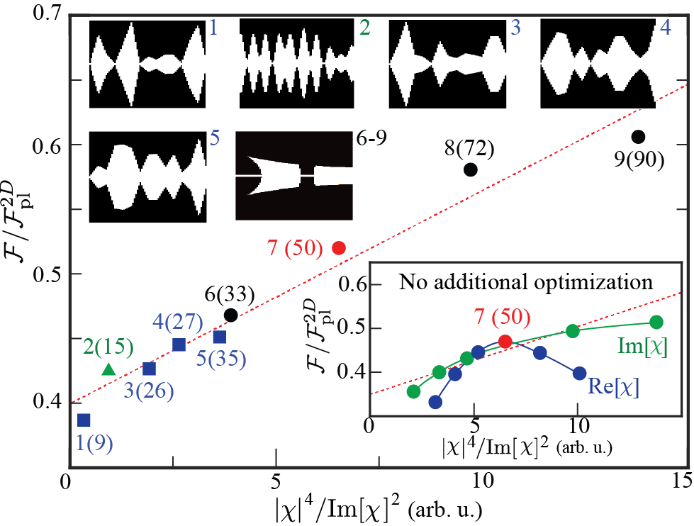
Figure 2: Observation of material scaling in shape optimization: The figure highlights the material trend in enhancement $\mathcal{F}/\mathcal{F}^{2D}_{\text{pl}}$ found by optimizing grating geometries over a wide range of material susceptibilities $\chi$. Quantities displayed in parenthesis correspond to the relative enhancement of a given grating design compared to a planar geometry of the same material. Various shape parameterizations such as polylines, Fourier curves, and ellipsoids marked as squares, triangles, and circles are considered. The susceptibility values are chosen to vary along either the real or imaginary axis: gratings $\{1,2,4\}$ correspond to $\chi=\{-76,-101,-151\}+50i$, $5$ to $\chi=-151+40i$, $\{3,7\}$ to $\chi=\{-121,169.5\}+37.3i$, and $\{6\rightarrow 9\}$ to $\chi=-169.5+\{50,37.3,30,25\}i$. Results for tungsten are colored red. The upper inset illustrates the unit cell of correspondingly numbered grating. (There is no visible difference for gratings 6-9 and so only one of these is shown.) The lower inset depicts the RHT of tungsten grating 7 when the susceptibility is varied without altering the structure. The dashed line represents the susceptibility scaling predicted by recently derived limits on RHT Miller et al. (2015).

We begin by considering tungsten gratings, which at $\lambda_{\text{opt}}$ exhibits a highly metallic response $\chi\approx-170+37i$ far from the planar SPP condition. Figure 1 depicts the spectral enhancement factor $\mathcal{F}/\mathcal{F}^{2D}_{\text{pl}}$ for both unstructured plates “$(0)$” and optimized gratings “$(N)$” obtained by successively increasing the number of (ellipsoidal) shapes allowed in each unit cell, $N$. The spectra of the two optimized gratings, illustrated as insets , both peak at $\lambda_{\text{opt}}$ (black dashed line), with magnitudes $\mathcal{F}/\mathcal{F}^{2D}_{\text{pl}}=\{0.40,0.53\}$ increasing with the number of ellipsoids, $\{1,3\}$. On the one hand, enhancements of this magnitude for lossy metals, $|\chi|/\mathrm{Im}\left(\chi\right)\gtrsim 1$, are considered challenging Raether (1988) at small separations, $d\ll\lambda_{\text{opt}}$. On the other hand, large RHT is known to be possible in ultra-thin films through the interference of coupled SPPs Guo et al. (2014). However, to reach the magnitudes obtained here, unrealistically small thicknesses $\lesssim 1$ nm are needed. In contrast, no feature in the gratings of Fig. 1 is smaller than $10$ nm. Notably, although the optimization is carried out at a single frequency, the discovered enhancement peaks are always broadband due to the high level of material absorption. Consequently, the frequency-integrated RHT at $T=1000$ K exhibited by grating $(3)$ is found to be roughly $10\%$ larger than that of two planar silicon carbide (black line), a low-loss polaritonic material. To explain this enhancement, Fig. 1 (right) examines the transfer function $\mathcal{T}(\omega,k)$ versus frequency and wavenumber $k$. In moving from (1) to (3), the color plot demonstrates (frequency axis) that additional modes are successively created and pushed towards $\omega_{\mathrm{opt}}$, enhancing the density of states. Owing to the large size of the BZ (small periodicity $\Lambda=0.04\;\lambda_{\text{opt}}$), we find that the range of rate matching achieved here is considerably larger than that observed in previously examined grating structures Dai et al. (2015).

Another key finding is depicted in Fig 2, which plots RHT enhancement for representative optimizations  across an array of material and geometry combinations, as a function of the material scaling factor $|\chi|^{4}/\text{Im}\left[\chi\right]^{2}$ of (1). Three different classes of design are explored: collections of ellipsoids (circles), single polyline interfaces (squares), and Fourier curves (triangles). Uniformly, every one of these structures is observed to enhance RHT by at least an order of magnitude compared to the corresponding planar systems and within factors of unity of the ideal planar bound, (3). Regardless of the particular parameterization, over the range of examined $\text{Re}[\chi]$ and $\text{Im}[\chi]$, a clear linear trend in $\mathcal{F}$ (red dotted line) as a function of $|\chi|^{4}/\text{Im}\left[\chi\right]^{2}$ is observed. This linear scaling becomes increasingly difficult to observe at larger values of $\chi$, where larger resolutions are needed to accurately capture resonant behavior and the optimization requires increasingly larger number of iterations to find structures along the fit line. As should be expected, based on the fact that this behavior has not been previously reported, material scaling consistent with (1) is seen only for gratings optimized specifically for each particular value of $\chi(\omega_{\mathrm{opt}})$. For a fixed geometry, Fig. 2 (insets), varying either $\text{Re}[\chi]$ or $\text{Im}[\chi]$ shifts the resonance away from $\omega_{\mathrm{opt}}$ and diminishes RHT. The appearance of this linear trend indicates that aspects of the arguments leading to the energy bounds inMiller et al. (2015) are coming into play. However, the fact that a substantial increase in available design space has failed to significantly bridge the magnitude gap suggests that approaching these bounds (at least in 2d) may prove challenging with practical structures. Conversely, it should be emphasized that our results do not preclude the existence of structures with much larger enhancements. First, although the design space we have investigated is substantially larger than previous work, it is still relatively limited. Second, the complexity of the strutures and degree of enhancement are limited by the spatial resolution of the chosen discretization, $0.0005\;\lambda_{\text{opt}}$ (1/40th of the gap size).

To summarize, in investigating potential radiative heat transfer enhancements through inverse design, we have found evidence supporting the material scaling recently predicted by shape-indepedent bounds Miller et al. (2015), a feature that to our knowledge had yet to be confirmed. While the observed heat transfer rates are still far from matching the magnitudes predicted by general bounds, we have found that RHT rates between fabricable tungsten gratings (a highly lossy metal), for subwavelength gap separations as small as $2\%$ of the design wavelength, can selectively approach $50\%$ of the rate achieved by ideal planar materials (lossless metals satisfying the SPP condition) in the infrared. The results represent nearly two orders of magnitude greater RHT rates in structured compared to planar materials. It remains to be seen to what degree similar strategies might enhance RHT in three dimensions, where the photonic density of states is larger and its associated dependence on material losses significantly stronger.

This work was supported by the National Science Foundation under Grant No. DMR-1454836, Grant No. DMR 1420541, and Award EFMA-1640986; and the National Science and Research Council of Canada under PDF-502958-2017.

Appendix A: Approximate Singular Value Decomposition

In this appendix, we sketch how the low-rank nature of the RHT matrix $\mathcal{Z}^{{}_{AB}}=\sqrt{\text{Im}\left[\chi^{{}_{A}}\right]}\mathcal{G}^{{}_{AB}}\sqrt{\text{Im}\left[\chi^{{}_{B}}\right]}$ entering (6) in the main text allows application of fast randomized singular value decompositions (SVD), greatly speeding up calculations of RHT. We begin by splitting the problem into two domains, referred to as bodies $A$ and $B$, with associated superscripts denoting projection. It will be assumed that sources occur in body $A$ and that the fields of interest lie only in body $B$. (From Lorentz reciprocity, the Green function must be symmetric under the exchange of observation and source positions, and so there is no loss of generality in either choice.) The algorithm, described in detail in Halko et al. (2011), proceeds iteratively as follows.

Draw a random Gaussian distributed current vector $\tilde{\textbf{j}}_{i+1}$ with values in body $A$. Let $\tilde{\Omega}_{i}^{{}_{A}}$ denote the set of all previously drawn randomly Gaussian distributed current vectors (vertically concatenated to form a matrix). Solve Maxwell equation’s to obtain the associated field, $\tilde{\mathbf{E}}_{i+1}=\mathcal{G}\tilde{\textbf{j}}_{i+1}$. Let $\tilde{O}^{{}_{B}}_{i}$ denote the set of all previously computed, orthonormalized, electromagnetic field vectors, and $\tilde{Y}^{{}_{B}}_{i}$ the set of all previous electromagnetic fields as originally calculated. Compute $\tilde{\textbf{o}}^{u\;_{B}}_{i+1}=\left(I-\tilde{O}^{{}_{B}}_{i}\tilde{O}^{\dagger_{B}}_{i}\right)\tilde{\mathbf{E}}_{i+1}$, and normalize the result $\tilde{\textbf{o}}^{{}_{B}}_{i+1}=\tilde{\textbf{o}}^{u_{B}}_{i+1}/\langle\tilde{\textbf{o}}^{u_{B}}_{i+1}|\tilde{\textbf{o}}^{u_{B}}_{i+1}\rangle$, recording the value of $\epsilon_{i+1}=\langle\tilde{\textbf{o}}^{u_{B}}_{i+1}|\tilde{\textbf{o}}^{u_{B}}_{i+1}\rangle$. Concatenate $\tilde{\textbf{o}}^{{}_{B}}_{i+1}$ onto $\tilde{O}^{{}_{B}}_{i}$ and $\tilde{\mathbf{E}}_{i+1}$ onto $\tilde{Y}^{{}_{B}}_{i}$, producing $\tilde{O}^{{}_{B}}_{i+1}$ and $\tilde{Y}^{{}_{B}}_{i+1}$. Similarly, draw random currents $\tilde{\textbf{j}}_{i+1}$ in body $B$ and repeat the previous procedure, producing $\tilde{O}^{{}_{A}}_{i+1}$ and $\tilde{Y}^{{}_{A}}_{i+1}$. The iterations are stopped when both $\epsilon_{i+1}$ and $\epsilon^{\dagger}_{i+1}$ (for both $A$ and $B$ calculations) are smaller than a prescribed singular value tolerance.

Given the above matrices, a low-rank approximation of the SVD of $\mathcal{Z}^{{}_{AB}}$ is obtained by expanding it onto the basis functions $\tilde{O}^{{}_{A}}$ and $\tilde{O}^{{}_{B}}$. From random matrix theory Halko et al. (2011), given that $\epsilon_{i+1}$ is small for a given number of successive iterations, this basis approximately spans the domain and range of the matrix. It follows from Maxwell’s equations that $\tilde{Y}^{{}_{A}}=\mathcal{G}^{{}_{AB}}\tilde{\Omega}^{{}_{B}}$ and hence,

$$\tilde{O}^{{}_{A}\dagger}\mathcal{Z}^{{}_{AB}}\tilde{O}^{{}_{B}}\tilde{O}^{{}_{B}\dagger}\sqrt{\text{Im}[\chi^{{}_{B}}]}^{-1}\tilde{\Omega}^{{}_{B}}\approx\tilde{O}^{{}_{A}\dagger}\sqrt{\text{Im}[\chi^{{}_{A}}]}\tilde{Y}^{{}_{A}}.$$

Multiplication by the inverse of $\tilde{O}^{{}_{B}\dagger}\sqrt{\text{Im}[\chi^{{}_{B}}]}^{-1}\tilde{\Omega}^{{}_{B}}$ then produces a low-dimension $k\times k$ matrix on the right hand side, amenable to standard SVD at minimal cost,

$$\tilde{O}^{{}_{A}\dagger}\mathcal{Z}^{{}_{AB}}\tilde{O}^{{}_{B}}\approx\underbrace{\tilde{O}^{{}_{A}\dagger}\sqrt{\text{Im}[\chi^{{}_{A}}]}\tilde{Y}^{{}_{A}}\left(\tilde{O}^{{}_{B}\dagger}\sqrt{\text{Im}[\chi^{{}_{B}}]}^{-1}\tilde{\Omega}^{{}_{B}}\right)^{-1}}_{U\Sigma V^{\dagger}}.$$ (8)

The singular value approximation of $\mathcal{Z}^{{}_{AB}}$ is then derived from the small $k\times k$ matrices $U$, $\Sigma$, and $V$,

$$\mathcal{Z}^{{}_{AB}} \approx\tilde{O}^{{}_{A}}U\Sigma V^{\dagger}\tilde{O}^{{}_{B}\dagger}$$

$$=\left(\tilde{O}^{{}_{A}}U\right)\Sigma\left(\tilde{O}^{{}_{B}}V\right)^{\dagger}$$ (9)

Analysis of the convergence and performance properties of similar algorithms have been previously produced in Halko et al. (2011).

Appendix B: Fast Gradient Adjoints

To exploit gradient-based optimization, knowledge of $\partial\Phi/\left(\partial p_{\alpha}\right)$ is required for each optimization parameter $p_{\alpha}$. Letting $\partial_{\alpha}$ denote a partial derivative with respect to $p_{\alpha}$, and retaining the notation of the main text and Appendix A,

$$\partial_{\alpha}\Phi =\frac{\omega^{4}\Theta}{2\pi c^{4}}\partial_{\alpha}\text{Tr}\left[\text{Im}\left[\chi^{{}_{B}}\right]\mathcal{G}^{{}_{AB}\dagger}\text{Im}\left[\chi^{{}_{A}}\right]\mathcal{G}^{{}_{AB}}\right].$$ (10)

Using the symmetry of $\chi^{{}_{A}}$ and $\chi^{{}_{B}}$, along with the usual cyclic properties of the trace,

$$\text{Tr}\left[\text{Im}\left[\chi^{{}_{B}}\right]\partial_{\alpha}\mathcal{G}^{{}_{AB}\dagger}\text{Im}\left[\chi^{{}_{A}}\right]\mathcal{G}^{{}_{AB}}\right]=$$

$$\text{Tr}\left[\mathcal{G}^{{}_{AB}\intercal}\text{Im}\left[\chi^{{}_{A}}\right]\partial_{\alpha}\mathcal{G}^{{}_{AB*}}\text{Im}\left[\chi^{{}_{B}}\right]\right]=$$

$$\text{Tr}\left[\text{Im}\left[\chi^{{}_{B}}\right]\mathcal{G}^{{}_{AB}\intercal}\text{Im}\left[\chi^{{}_{A}}\right]\partial_{\alpha}\mathcal{G}^{{}_{AB*}}\right],$$

one finds that the second and fourth terms in the partial derivative expansion are complex conjugates. (Here, $\intercal$ denotes transposition without complex conjugation.) Given that $\mathcal{G}=\left[\left(\nabla\times\nabla\times\right)-\omega^{2}\epsilon\right]^{-1}$ is the inverse Maxwell operator,

$$\partial_{\alpha}\mathcal{G}^{{}_{AB}}=\omega^{2}\;\mathcal{G}^{{}_{A}\cdot}\partial_{\alpha}\chi\;\mathcal{G}^{\cdot_{B}},$$

and so one finds:

$$\partial_{\alpha}\Phi=\frac{\omega^{4}\Theta}{2\pi c^{4}}\text{Tr}\Bigg{[}\mathcal{G}^{{}_{AB}\dagger}\text{Im}\left[\chi^{{}_{A}}\right]\mathcal{G}^{{}_{AB}}\text{Im}\left[\partial_{\alpha}\chi^{{}_{B}}\right]+$$

$$\mathcal{G}^{{}_{AB}}\text{Im}\left[\chi^{{}_{B}}\right]\mathcal{G}^{{}_{AB}\dagger}\text{Im}\left[\partial_{\alpha}\chi^{{}_{A}}\right]+$$

$$2\omega^{2}\text{Re}\left[\mathcal{G}^{\cdot_{B}}\text{Im}\left[\chi^{{}_{B}}\right]\mathcal{G}^{{}_{AB}\dagger}\text{Im}\left[\chi^{{}_{A}}\right]\mathcal{G}^{{}_{A}\cdot}\partial_{\alpha}\chi\right]\Bigg{]}.$$ (11)

The $\mathcal{G}^{{}_{AB}}$ matrices involved in (11) are low rank, and can computed alongside $\mathcal{Z}^{{}_{AB}}$ at almost no extra cost. Specifically, if $\sqrt{\text{Im}\left[\chi^{{}_{A}}\right]}$ and $\sqrt{\text{Im}\left[\chi^{{}_{B}}\right]}$ are excluded from the error estimates $\epsilon_{i+1}$ and $\epsilon^{\dagger}_{i+1}$, one obtains an approximation for $\mathcal{G}^{{}_{BA}}$ rather than $\mathcal{Z}^{{}_{AB}}$. Both computations can be carried out at the same time, using the same current sources and field solutions. If these matrices have rank $k$, the parameter independent matrices of (11) are solved in order $k$ computations. Hence, determination of the gradient is essentially no more costly than the determination of $\Phi$.

References

- Kittel et al. (2005) A. Kittel, W. Müller-Hirsch, J. Parisi, S.-A. Biehs, D. Reddig, and M. Holthaus, Physical Review Letters 95, 224301 (2005).
- Kim et al. (2015) K. Kim, B. Song, V. Fernández-Hurtado, W. Lee, W. Jeong, L. Cui, D. Thompson, J. Feist, M. H. Reid, F. J. García-Vidal, et al., Nature 528, 387 (2015).
- Song et al. (2015) B. Song, Y. Ganjeh, S. Sadat, D. Thompson, A. Fiorino, V. Fernández-Hurtado, J. Feist, F. J. Garcia-Vidal, J. C. Cuevas, P. Reddy, et al., Nature Nanotechnology 10, 253 (2015).
- St-Gelais et al. (2016) R. St-Gelais, L. Zhu, S. Fan, and M. Lipson, Nature Nanotechnology 11, 515 (2016).
- Pendry (1999) J. Pendry, Journal of Physics: Condensed Matter 11, 6621 (1999).
- Carminati and Greffet (1999) R. Carminati and J.-J. Greffet, Physical Review Letters 82, 1660 (1999).
- Volokitin and Persson (2001) A. Volokitin and B. Persson, Physical Review B 63, 205404 (2001).
- Babuty et al. (2013) A. Babuty, K. Joulain, P.-O. Chapuis, J.-J. Greffet, and Y. De Wilde, Physical Review Letters 110, 146103 (2013).
- Narayanaswamy and Chen (2003) A. Narayanaswamy and G. Chen, Applied Physics Letters 82, 3544 (2003).
- Laroche et al. (2006) M. Laroche, R. Carminati, and J.-J. Greffet, Journal of Applied Physics 100, 063704 (2006).
- Park et al. (2008) K. Park, S. Basu, W. P. King, and Z. Zhang, Journal of Quantitative Spectroscopy and Radiative Transfer 109, 305 (2008).
- Ilic et al. (2012) O. Ilic, M. Jablan, J. D. Joannopoulos, I. Celanovic, and M. Soljačić, Optics Express 20, A366 (2012).
- Karalis and Joannopoulos (2017) A. Karalis and J. Joannopoulos, Scientific Reports 7, 14046 (2017).
- St-Gelais et al. (2017) R. St-Gelais, G. R. Bhatt, L. Zhu, S. Fan, and M. Lipson, ACS Nano 11, 3001 (2017).
- Guha et al. (2012) B. Guha, C. Otey, C. B. Poitras, S. Fan, and M. Lipson, Nano Letters 12, 4546 (2012).
- Yang et al. (2013) Y. Yang, S. Basu, and L. Wang, Applied Physics Letters 103, 163101 (2013).
- Khandekar et al. (2018) C. Khandekar, R. Messina, and A. W. Rodriguez, AIP Advances 8, 055029 (2018).
- Challener et al. (2009) W. Challener, C. Peng, A. Itagi, D. Karns, W. Peng, Y. Peng, X. Yang, X. Zhu, N. Gokemeijer, Y.-T. Hsia, et al., Nature Photonics 3, 220 (2009).
- Bhargava and Yablonovitch (2015) S. Bhargava and E. Yablonovitch, IEEE Transactions on Magnetics 51, 3100407 (2015).
- Volokitin and Persson (2007) A. Volokitin and B. N. Persson, Rev. Mod. Phys. 79, 1291 (2007).
- Iizuka and Fan (2015) H. Iizuka and S. Fan, Physical Review B 92, 144307 (2015).
- Domoto et al. (1970) G. Domoto, R. Boehm, and C. L. Tien, Journal of Heat Transfer 92, 412 (1970).
- Kralik et al. (2012) T. Kralik, P. Hanzelka, M. Zobac, V. Musilova, T. Fort, and M. Horak, Physical Review Letters 109, 224302 (2012).
- Ijiro and Yamada (2015) T. Ijiro and N. Yamada, Applied Physics Letters 106, 023103 (2015).
- Lang et al. (2017) S. Lang, G. Sharma, S. Molesky, P. U. Kränzien, T. Jalas, Z. Jacob, A. Y. Petrov, and M. Eich, Scientific Reports 7, 13916 (2017).
- Shen et al. (2009) S. Shen, A. Narayanaswamy, and G. Chen, Nano Letters 9, 2909 (2009).
- Luo and Chen (2013) T. Luo and G. Chen, Physical Chemistry Chemical Physics 15, 3389 (2013).
- Basu et al. (2007) S. Basu, Y.-B. Chen, and Z. Zhang, International Journal of Energy Research 31, 689 (2007).
- Rephaeli and Fan (2009) E. Rephaeli and S. Fan, Optics Express 17, 15145 (2009).
- Molesky et al. (2013) S. Molesky, C. J. Dewalt, and Z. Jacob, Optics Express 21, A96 (2013).
- Nagpal et al. (2011) P. Nagpal, D. P. Josephson, N. R. Denny, J. DeWilde, D. J. Norris, and A. Stein, Journal of Materials Chemistry 21, 10836 (2011).
- Rinnerbauer et al. (2013) V. Rinnerbauer, Y. X. Yeng, W. R. Chan, J. J. Senkevich, J. D. Joannopoulos, M. Soljačić, and I. Celanovic, Optics Express 21, 11482 (2013).
- Dyachenko et al. (2016) P. Dyachenko, S. Molesky, A. Y. Petrov, M. Störmer, T. Krekeler, S. Lang, M. Ritter, Z. Jacob, and M. Eich, Nature Communications 7 (2016).
- Miller et al. (2015) O. D. Miller, S. G. Johnson, and A. W. Rodriguez, Physical Review Letters 115, 204302 (2015).
- Fernández-Hurtado et al. (2017) V. Fernández-Hurtado, F. J. Garcia-Vidal, S. Fan, and J. C. Cuevas, Physical Review Letters 118, 203901 (2017).
- Dai et al. (2017) J. Dai, F. Ding, S. I. Bozhevolnyi, and M. Yan, Physical Review B 95, 245405 (2017).
- Guérout et al. (2012) R. Guérout, J. Lussange, F. Rosa, J.-P. Hugonin, D. Dalvit, J.-J. Greffet, A. Lambrecht, and S. Reynaud, in Journal of Physics: Conference Series, Vol. 395 (IOP Publishing, 2012) p. 012154.
- Lussange et al. (2012) J. Lussange, R. Guérout, F. S. Rosa, J.-J. Greffet, A. Lambrecht, and S. Reynaud, Physical Review B 86, 085432 (2012).
- Liu and Shen (2013) B. Liu and S. Shen, Physical Review B 87, 115403 (2013).
- Jin et al. (2017) W. Jin, R. Messina, and A. W. Rodriguez, Optics Express 25, 293277 (2017).
- Molesky et al. (2018) S. Molesky, Z. Lin, A. Y. Piggott, W. Jin, J. Vuckovic, and A. W. Rodriguez, arXiv:1801.06715 (2018).
- Pralle et al. (2002) M. Pralle, N. Moelders, M. McNeal, I. Puscasu, A. Greenwald, J. Daly, E. Johnson, T. George, D. Choi, I. El-Kady, et al., Applied Physics Letters 81, 4685 (2002).
- De Zoysa et al. (2012) M. De Zoysa, T. Asano, K. Mochizuki, A. Oskooi, T. Inoue, and S. Noda, Nature Photonics 6, 535 (2012).
- Liu et al. (2010) N. Liu, M. Mesch, T. Weiss, M. Hentschel, and H. Giessen, Nano Letters 10, 2342 (2010).
- Rodriguez et al. (2011) A. W. Rodriguez, O. Ilic, P. Bermel, I. Celanovic, J. D. Joannopoulos, M. Soljačić, and S. G. Johnson, Physical Review Letters 107, 114302 (2011).
- Rodriguez et al. (2012) A. W. Rodriguez, M. H. Reid, and S. G. Johnson, Physical Review B 86, 220302 (2012).
- Otey et al. (2014) C. R. Otey, L. Zhu, S. Sandhu, and S. Fan, Journal of Quantitative Spectroscopy and Radiative Transfer 132, 3 (2014).
- Messina et al. (2017) R. Messina, A. Noto, B. Guizal, and M. Antezza, Physical Review B 95, 125404 (2017).
- Boyd and Vandenberghe (2004) S. Boyd and L. Vandenberghe, Convex Optimization (Cambridge University Press, 2004).
- Edalatpour and Francoeur (2016) S. Edalatpour and M. Francoeur, Physical Review B 94, 045406 (2016).
- Liu et al. (2015a) X. Liu, L. Wang, and Z. M. Zhang, Nanoscale and Microscale Thermophysical Engineering 19, 98 (2015a).
- Biehs et al. (2011) S.-A. Biehs, P. Ben-Abdallah, F. S. Rosa, K. Joulain, and J.-J. Greffet, Optics Express 19, A1088 (2011).
- Guo et al. (2012) Y. Guo, C. L. Cortes, S. Molesky, and Z. Jacob, Applied Physics Letters 101, 131106 (2012).
- Liu et al. (2013) X. Liu, R. Zhang, and Z. Zhang, Applied Physics Letters 103, 213102 (2013).
- Liu et al. (2014) X. Liu, R. Zhang, and Z. Zhang, International Journal of Heat and Mass Transfer 73, 389 (2014).
- Shi et al. (2015) J. Shi, B. Liu, P. Li, L. Y. Ng, and S. Shen, Nano Letters 15, 1217 (2015).
- Didari and Mengüç (2015) A. Didari and M. P. Mengüç, Optics Express 23, A1253 (2015).
- Ben-Abdallah et al. (2009) P. Ben-Abdallah, K. Joulain, J. Drevillon, and G. Domingues, Journal of Applied Physics 106, 044306 (2009).
- Francoeur et al. (2010) M. Francoeur, M. P. Mengüç, and R. Vaillon, Journal of Physics D: Applied Physics 43, 075501 (2010).
- Basu and Francoeur (2011) S. Basu and M. Francoeur, Applied Physics Letters 98, 243120 (2011).
- Van Zwol et al. (2011) P. Van Zwol, K. Joulain, P. Ben-Abdallah, and J. Chevrier, Physical Review B 84, 161413 (2011).
- Pendharker et al. (2017) S. Pendharker, H. Hu, S. Molesky, R. Starko-Bowes, Z. Poursoti, S. Pramanik, N. Nazemifard, R. Fedosejevs, T. Thundat, and Z. Jacob, Journal of Optics 19, 055101 (2017).
- Naik et al. (2013) G. V. Naik, V. M. Shalaev, and A. Boltasseva, Advanced Materials 25, 3264 (2013).
- Chalabi et al. (2016) H. Chalabi, A. Alù, and M. L. Brongersma, Physical Review B 94, 094307 (2016).
- Liu and Zhang (2015) X. Liu and Z. Zhang, ACS Photonics 2, 1320 (2015).
- Zheng et al. (2018) Z. Zheng, A. Wang, and Y. Xuan, Journal of Quantitative Spectroscopy and Radiative Transfer (2018).
- Liu and Zhang (2014) X. L. Liu and Z. M. Zhang, Applied Physics Letters 104, 251911 (2014).
- Dai et al. (2015) J. Dai, S. A. Dyakov, and M. Yan, Physical Review B 92, 035419 (2015).
- Liu et al. (2015b) X. Liu, B. Zhao, and Z. M. Zhang, Phys. Rev. A 91, 062510 (2015b).
- Note (1) There is a considerable body of work in this area. The accuracy of effective medium approximations has been explored for both one- and two-dimensional grating structures, with and without dielectric filling Dai2; Dai3.
- Prodan et al. (2003) E. Prodan, C. Radloff, N. J. Halas, and P. Nordlander, science 302, 419 (2003).
- Biehs et al. (2010) S.-A. Biehs, E. Rousseau, and J.-J. Greffet, Physical Review Letters 105, 234301 (2010).
- Chalabi et al. (2015) H. Chalabi, E. Hasman, and M. L. Brongersma, Physical Review B 91, 174304 (2015).
- Baldwin et al. (2014) C. L. Baldwin, N. W. Bigelow, and D. J. Masiello, Journal of Physical Chemistry Letters 5, 1347 (2014).
- Pérez-Rodríguez et al. (2017) J. E. Pérez-Rodríguez, G. Pirruccio, and R. Esquivel-Sirvent, Physical Review Materials 1, 062201 (2017).
- Molesky and Jacob (2015) S. Molesky and Z. Jacob, Physical Review B 91, 205435 (2015).
- Liu et al. (2017) B. Liu, J. Li, and S. Shen, ACS Photonics (2017).
- Wang and Menon (2013) P. Wang and R. Menon, Optics Express 22, A99 (2013).
- Ganapati et al. (2014) V. Ganapati, O. D. Miller, and E. Yablonovitch, IEEE Journal of Photovoltaics 4, 175 (2014).
- Diem et al. (2009) M. Diem, T. Koschny, and C. M. Soukoulis, Physical Review B 79, 033101 (2009).
- Hedayati et al. (2011) M. K. Hedayati, M. Javaherirahim, B. Mozooni, R. Abdelaziz, A. Tavassolizadeh, V. S. K. Chakravadhanula, V. Zaporojtchenko, T. Strunkus, F. Faupel, and M. Elbahri, Advanced Materials 23, 5410 (2011).
- Nguyen et al. (2017) D. M. Nguyen, D. Lee, and J. Rho, Scientific Reports 7, 2611 (2017).
- Rytov et al. (1988) S. M. Rytov, Y. A. Kravtsov, and V. I. Tatarskii, (1988).
- Kong (1975) J. A. Kong, New York, Wiley-Interscience, 1975. 348 p. (1975).
- Li and Demmel (2003) X. S. Li and J. W. Demmel, ACM Transactions on Mathematical Software (TOMS) 29, 110 (2003).
- Plessix (2007) R.-E. Plessix, Geophysics 72, SM185 (2007).
- Gatto and Hesthaven (2015) P. Gatto and J. S. Hesthaven, arXiv preprint arXiv:1508.07798 (2015).
- Halko et al. (2011) N. Halko, P.-G. Martinsson, and J. A. Tropp, SIAM review 53, 217 (2011).
- Caers and Hoffman (2006) J. Caers and T. Hoffman, Mathematical Geology 38, 81 (2006).
- Martinez-Cantin (2014) R. Martinez-Cantin, The Journal of Machine Learning Research 15, 3735 (2014).
- Tsuji and Hirayama (2008) Y. Tsuji and K. Hirayama, IEEE photonics technology letters 20, 982 (2008).
- Xu et al. (2003) F. Xu, Y. Zhang, W. Hong, K. Wu, and T. J. Cui, IEEE Transactions on Microwave Theory and Techniques 51, 2221 (2003).
- Note (2) Full geometric characterizations of these structures and those presented later in the text are available upon request.
- Note (3) The optimizations involving four elliptical bodies usually require iterations to reach convergence; roughly hours of total computation time for each structure.
- Raether (1988) H. Raether, in Surface plasmons on smooth and rough surfaces and on gratings (Springer, 1988) pp. 91–116.
- Guo et al. (2014) Y. Guo, S. Molesky, H. Hu, C. L. Cortes, and Z. Jacob, Applied Physics Letters 105, 073903 (2014).
- Note (4) The structures with the best performance features over all trials with the same susceptibility.