Orthogonality-Promoting Distance Metric Learning: Convex Relaxation and Theoretical Analysis

Abstract

Distance metric learning (DML), which learns a distance metric from labeled “similar” and “dissimilar” data pairs, is widely utilized. Recently, several works investigate orthogonality-promoting regularization (OPR), which encourages the projection vectors in DML to be close to being orthogonal, to achieve three effects: (1) high balancedness – achieving comparable performance on both frequent and infrequent classes; (2) high compactness – using a small number of projection vectors to achieve a “good” metric; (3) good generalizability – alleviating overfitting to training data. While showing promising results, these approaches suffer three problems. First, they involve solving non-convex optimization problems where achieving the global optimal is NP-hard. Second, it lacks a theoretical understanding why OPR can lead to balancedness. Third, the current generalization error analysis of OPR is not directly on the regularizer. In this paper, we address these three issues by (1) seeking convex relaxations of the original nonconvex problems so that the global optimal is guaranteed to be achievable; (2) providing a formal analysis on OPR’s capability of promoting balancedness; (3) providing a theoretical analysis that directly reveals the relationship between OPR and generalization performance. Experiments on various datasets demonstrate that our convex methods are more effective in promoting balancedness, compactness, and generalization, and are computationally more efficient, compared with the nonconvex methods.

1 Introduction

Given data pairs labeled as either “similar” or “dissimilar”, distance metric learning [58, 51, 11] learns a distance measure in such a way that similar examples are placed close to each other while dissimilar ones are separated apart. The learned distance metrics are important to many downstream tasks, such as retrieval [9], classification [51] and clustering [58]. One commonly used distance metric between two examples $\mathbf{x},\mathbf{y}\in\mathbb{R}^{D}$ is: $\|\mathbf{A}\mathbf{x}-\mathbf{A}\mathbf{y}\|_{2}$ [51, 55, 9], which is parameterized by $R$ projection vectors (in $\mathbf{A}\in\mathbb{R}^{R\times D})$.

Many works [50, 55, 48, 42, 9] have proposed orthogonality-promoting DML to learn distance metrics that are (1) balanced: performing equally well on data instances belonging to frequent and infrequent classes; (2) compact: using a small number of projection vectors to achieve a “good” metric, (i.e., capturing well the relative distances of the data pairs); (3) generalizable: reducing the overfitting to training data. Regarding balancedness, under many circumstances, the frequency of classes, defined as the number of examples belonging to each class, can be highly imbalanced. Classic DML methods are sensitive to the skewness of the frequency of the classes: they perform favorably on frequent classes whereas less well on infrequent classes — a phenomenon also confirmed in our experiments in Section 7. However, infrequent classes are of crucial importance in many applications, and should not be ignored. For example, in a clinical setting, many diseases occur infrequently, but are life-threatening. Regarding compactness, the number of the projection vectors $R$ entails a tradeoff between performance and computational complexity [16, 55, 42]. On one hand, more projection vectors bring in more expressiveness in measuring distance. On the other hand, a larger $R$ incurs a higher computational overhead since the number of weight parameters in $\mathbf{A}$ grows linearly with $R$. It is therefore desirable to keep $R$ small without hurting much ML performance. Regarding generalization performance, in the case where the sample size is small but the size of $\mathbf{A}$ is large, overfitting can easily happen.

To address these three issues, many studies [58, 51, 11, 20, 61, 25, 63] propose to regularize the projection vectors to be close to being orthogonal. For balancedness, they argue that, without orthogonality-promoting regularization (OPR), the majority of projection vectors learn latent features for frequent classes since these classes have dominant signals in the dataset; through OPR, the projection vectors uniformly “spread out”, giving both infrequent and frequent classes a fair treatment and thus leading to a more balanced distance metric (see [57] for details). For compactness, they claim that: “diversified” projection vectors bear less redundancy and are mutually complementary; as a result, a small number of such vectors are sufficient to achieve a “good” distance metric. For generalization performance, they posit that OPR imposes a structured constraint on the function class of DML, hence reduces model complexity.

While these orthogonality-promoting DML methods have shown promising results, they have three problems. First, they involve solving non-convex optimization problems where the global solution is extremely difficult, if not impossible, to obtain. Second, no formal analysis is conducted regarding why OPR can promote balancedness. Third, while the generalization error (GE) analysis of OPR has been studied in [57], it is incomplete. In this analysis, they first show that the upper bound of GE is a function of cosine similarity (CS), then show that CS and the regularizer are somewhat aligned in shape. They did not establish a direct relationship between the GE bound and the regularizer.

In this paper, we aim at addressing these problems by making the following contributions:

• We relax the nonconvex, orthogonality-promoting DML problems into convex problems and develop efficient proximal gradient descent algorithms. The algorithms only run once with a single initialization, and hence are much more efficient than existing non-convex methods.

• We perform theoretical analysis which formally reveals the relationship between OPR and balancedness: stronger OPR leads to more balancedness.

• We perform generalization error (GE) analysis which shows that reducing the convex orthogonality-promoting regularizers can reduce the upper bound of GE.

• We apply the learned distance metrics for information retrieval to healthcare, texts, images, and sensory data. Compared with non-convex baseline methods, our approaches achieve higher computational efficiency and are more capable of improving balancedness, compactness and generalizability.

2 Related Works

2.1 Distance Metric Learning

Many studies [58, 51, 11, 20, 61, 25, 63] have investigated DML. Please refer to [28, 49] for a detailed review. Xing et al. [58] learn a Mahalanobis distance by minimizing the sum of distances of all similar data pairs subject to the constraint that the sum of all dissimilar pairs is no less than 1. Weinberger et al. [51] propose large margin metric learning, which is applied for k-nearest neighbor classification. For each data example $\mathbf{x}_{i}$, they first obtain $l$ nearest neighbors based on Euclidean distance. Among the $l$ neighbors, some (denoted by $\mathbf{S}=\{\mathbf{x}_{j}\}$) have the same class label with $\mathbf{x}_{i}$ and others (denoted by $D=\{\mathbf{x}_{k}\}$) do not. Then a projection matrix $\mathbf{L}$ is learned such that $\|\mathbf{L}(\mathbf{x}_{i}-\mathbf{x}_{k})\|_{2}^{2}-\|\mathbf{L}(\mathbf{x}_{i}-\mathbf{x}_{j})\|_{2}^{2}\geq 1$ where $\mathbf{x}_{j}\in\mathbf{S}$ and $\mathbf{x}_{k}\in\mathbf{D}$. Davis et al. [11] learn a Mahalanobis distance such that the distance between similar pairs is no more than a threshold $s$ and the distance between dissimilar pairs is no greater than a threshold $t$. Guillaumin et al. [20] define a probability of the similarity/dissimilarity label conditioned on the Mahalanobis distance: $p(y_{ij}|(\mathbf{x}_{i}-\mathbf{x}_{j})^{\top}\mathbf{M}(\mathbf{x}_{i}-\mathbf{x}_{j}))=1/(1+\exp((\mathbf{x}_{i}-\mathbf{x}_{j})^{\top}\mathbf{M}(\mathbf{x}_{i}-\mathbf{x}_{i})))$, where the binary variable $y_{ij}$ equals to 1 if $\mathbf{x}_{i}$ and $\mathbf{x}_{j}$ have the same class label. $\mathbf{M}$ is learned by maximizing the conditional likelihood of the training data. Kostinger et al. [25] learn a Mahalanobis distance metric from equivalence constraints based on likelihood ratio test. The Mahalanobis matrix is computed in one shot, without going through an iterative optimization procedure. Ying and Li [61] formulate DML as an eigenvalue optimization problem. Zadeh et al. [63] propose a geometric mean metric learning approach, based on the Riemannian geometry of positive definite matrices. Similar to [25], the Mahalanobis matrix has a closed form solution without iterative optimization.

To avoid overfitting in DML, various regularization approaches have been explored. Davis et al. [11] regularize the Mahalanobis matrix to be close to another matrix that encodes prior information, where the closeness is measured using log-determinant divergence. Qi et al. [40] use $\ell_{1}$ regularization to learn sparse distance metrics for high-dimensional, small-sample problems. Ying et al. [60] use $\ell_{2,1}$ norm to simultaneously encourage low-rankness and sparsity. Trace norm is leveraged to encourage low-rankness in [37, 32]. Qian et al. [41] apply dropout to DML. Many works [50, 16, 55, 59, 42, 9] study diversity-promoting regularization in DML or hashing. They define regularizers based on squared Frobenius norm [50, 13, 16, 9] or angles [55, 59] to encourage the projection vectors to approach orthogonal. Several works [31, 52, 18, 22, 48] impose strict orthogonal constraint on the projection vectors. As observed in previous works [50, 13] and our experiments, strict orthogonality hurts performance. Isotropic hashing [24, 15] encourages the variances of different projected dimensions to be equal to achieve balance. Carreira-Perpinán and Raziperchikolaei [8] propose a diversity hashing method which first trains hash functions independently and then introduces diversity among them based on classifier ensembles.

2.2 Orthogonality-Promoting Regularization

Orthogonality-promoting regularization has been studied in other problems as well, including ensemble learning, latent variable modeling, classification and multitask learning. In ensemble learning, many studies [30, 2, 39, 62] promote orthogonality among the coefficient vectors of base classifiers or regressors, with the aim to improve generalization performance and reduce computational complexity. Recently, several works [65, 3, 10, 56] study orthogonality-promoting regularization of latent variable models (LVMs), which encourages the components in LVMs to be mutually orthogonal, for the sake of capturing infrequent patterns and reducing the number of components without sacrificing modeling power. In these works, various orthogonality-promoting regularizers have been proposed, based on determinantal point process [27, 65] and cosine similarity [62, 3, 56]. In multi-way classification, Malkin and Bilmes [33] propose to use the determinant of a covariance matrix to encourage orthogonality among classifiers. Jalali et al. [21] propose a class of variational Gram functions (VGFs) to promote pairwise orthogonality among vectors. While these VGFs are convex, they can only be applied to non-convex DML formulations. As a result, the overall regularized DML is non-convex and is not amenable for convex relaxation.

In the sequel, we review two families of orthogonality-promoting regularizers.

Determinantal Point Process

[65] employed the determinantal point process (DPP) [27] as a prior to induce orthogonality in latent variable models. DPP is defined over $K$ vectors: $p(\{\mathbf{a}_{i}\}_{i=1}^{K})\propto\textrm{det}(\mathbf{L})$, where $\mathbf{L}$ is a $K\times K$ kernel matrix with $L_{ij}=k(\mathbf{a}_{i},\mathbf{a}_{j})$ and $k(\cdot,\cdot)$ as a kernel function. $\textrm{det}(\cdot)$ denotes the determinant of a matrix. A configuration of $\{\mathbf{a}_{i}\}_{i=1}^{K}$ with larger probability is deemed to be more orthogonal. The underlying intuition is that: $\textrm{det}(\mathbf{L})$ represents the volume of the parallelepiped formed by vectors in the kernel-induced feature space. If these vectors are closer to being orthogonal, the volume is larger, which results in a larger $p(\{\mathbf{a}_{i}\}_{i=1}^{K})$. The shortcoming of DPP is that it is sensitive to vector scaling. Enlarging the magnitudes of vectors results in larger volume, but does not essentially affects the orthogonality of vectors.

Pairwise Cosine Similarity

Several works define orthogonality-promoting regularizers based on the pairwise cosine similarity among component vectors: if the cosine similarity scores are close to zero, then the components are closer to being orthogonal. Given $K$ component vectors, the cosine similarity $s_{ij}$ between each pair of components $\mathbf{a}_{i}$ and $\mathbf{a}_{j}$ is computed: $s_{ij}=\mathbf{a}_{i}\cdot\mathbf{a}_{j}/(\|\mathbf{a}_{i}\|_{2}\|\mathbf{a}_{j}\|_{2})$. Then these scores are aggregated as a single score. In [62], these scores are aggregated as $\sum_{1\leq i<j\leq K}(1-s_{ij})$. In [3], the aggregation is performed as $-\log(\frac{1}{K(K-1)}\sum_{1\leq i<j\leq K}\beta|s_{ij}|)^{\frac{1}{\beta}}$ where $\beta>0$. In [56], the aggregated score is defined as mean of $\arccos(|s_{ij}|)$ minus the variance of $\arccos(|s_{ij}|)$.

3 Preliminaries

We review a DML method [57] that uses BMD [29] to promote orthogonality.

Distance Metric Learning

Given data pairs labeled either as “similar” $\mathcal{S}=\{(\mathbf{x}_{i},\mathbf{y}_{i})\}_{i=1}^{|\mathcal{S}|}$ or “dissimilar” $\mathcal{D}=\{(\mathbf{x}_{i},\mathbf{y}_{i})\}_{i=1}^{|\mathcal{D}|}$, DML [58, 51, 11] aims to learn a distance metric under which similar examples are close to each other and dissimilar ones are separated far apart. There are many ways to define a distance metric. Here, we present two popular choices. One is based on linear projection [51, 55, 9]. Given two examples $\mathbf{x},\mathbf{y}\in\mathbb{R}^{D}$, a linear projection matrix $\mathbf{A}\in\mathbb{R}^{R\times D}$ can be utilized to map them into a $R$-dimensional latent space. The distance metric is then defined as their squared Euclidean distance in the latent space: $\|\mathbf{Ax}-\mathbf{Ay}\|_{2}^{2}$. $\mathbf{A}$ can be learned by minimizing [58]: $\frac{1}{|\mathcal{S}|}\sum_{(\mathbf{x},\mathbf{y})\in\mathcal{S}}\|\mathbf{Ax}-\mathbf{Ay}\|_{2}^{2}+\frac{1}{|\mathcal{D}|}\sum_{(\mathbf{x},\mathbf{y})\in\mathcal{D}}\textrm{max}(0,\tau-\|\mathbf{Ax}-\mathbf{Ay}\|_{2}^{2})$, which aims at making the distances between similar examples as small as possible while separating dissimilar examples with a margin $\tau$ using a hinge loss. We call this formulation as projection matrix-based DML (PDML). PDML is a non-convex problem where the global optimal is difficult to achieve. Moreover, one needs to manually tune the number of projection vectors, typically via cross-validation, which incurs substantial computational overhead.

The other popular choice of distance metric is $(\mathbf{x}-\mathbf{y})^{\top}\mathbf{M}(\mathbf{x}-\mathbf{y})$, which is cast from $\|\mathbf{Ax}-\mathbf{Ay}\|_{2}^{2}$ by replacing $\mathbf{A}^{\top}\mathbf{A}$ with a positive semidefinite (PSD) matrix $\mathbf{M}$. This is known as the Mahalanobis distance [58]. Correspondingly, the PDML formulation can be transformed into a Mahalanobis distance-based DML (MDML) problem: $\textrm{min}_{\mathbf{M}\succeq 0}\;\frac{1}{|\mathcal{S}|}\sum_{(\mathbf{x},\mathbf{y})\in\mathcal{S}}(\mathbf{x}-\mathbf{y})^{\top}\mathbf{M}(\mathbf{x}-\mathbf{y})+\frac{1}{|\mathcal{D}|}\sum_{(\mathbf{x},\mathbf{y})\in\mathcal{D}}\textrm{max}(0,\tau-(\mathbf{x}-\mathbf{y})^{\top}\mathbf{M}(\mathbf{x}-\mathbf{y}))$, which is a convex problem where the global solution is guaranteed to be achievable. It also avoids tuning the number of projection vectors. However, the drawback of this approach is that, in order to satisfy the PSD constraint, one needs to perform eigen-decomposition of $\mathbf{M}$ in each iteration, which incurs $O(D^{3})$ complexity.

Orthogonality-Promoting Regularization

Among the various orthogonality-promoting regularizers, we choose the BMD [29] regularizer [57] in this study since it is amenable for convex relaxation and facilitates theoretical analysis.

To encourage orthogonality between two vectors $\mathbf{a}_{i}$ and $\mathbf{a}_{j}$, one can make their inner product $\mathbf{a}_{i}^{\top}\mathbf{a}_{j}$ close to zero and their $\ell_{2}$ norm $\|\mathbf{a}_{i}\|_{2}$, $\|\mathbf{a}_{j}\|_{2}$ close to one. For a set of vectors $\{\mathbf{a}_{i}\}_{i=1}^{R}$, their near-orthogonality can be achieved by computing the Gram matrix $\mathbf{G}$ where $G_{ij}=\mathbf{a}_{i}^{\top}\mathbf{a}_{j}$, then encouraging $\mathbf{G}$ to be close to an identity matrix. Off the diagonal of $\mathbf{G}$ and $\mathbf{I}$ are $\mathbf{a}_{i}^{\top}\mathbf{a}_{j}$ and zero, respectively. On the diagonal of $\mathbf{G}$ and $\mathbf{I}$ are $\|\mathbf{a}_{i}\|_{2}^{2}$ and one, respectively. Making $\mathbf{G}$ close to $\mathbf{I}$ effectively encourages $\mathbf{a}_{i}^{\top}\mathbf{a}_{j}$ to be close to zero and $\|\mathbf{a}_{i}\|_{2}$ close to one, which therefore encourages $\mathbf{a}_{i}$ and $\mathbf{a}_{j}$ to be close to orthogonal.

BMDs can be used to measure the “closeness” between two matrices. Let $\mathbf{S}^{n}$ denote real symmetric $n\times n$ matrices. Given a strictly convex, differentiable function $\phi:\mathbf{S}^{n}\to\mathbb{R}$, a BMD is defined as $\Gamma_{\phi}(\mathbf{X},\mathbf{Y})=\phi(\mathbf{X})-\phi(\mathbf{Y})-\text{tr}((\bigtriangledown\phi(\mathbf{Y}))^{\top}(\mathbf{X}-\mathbf{Y}))$, where $\text{tr}(\mathbf{A})$ denotes the trace of matrix $\mathbf{A}$. Different choices of $\phi(\mathbf{X})$ lead to different divergences. When $\phi(\mathbf{X})=\|\mathbf{X}\|_{F}^{2}$, the BMD is specialized to the squared Frobenius norm (SFN) $\|\mathbf{X}-\mathbf{Y}\|_{F}^{2}$. If $\phi(\mathbf{X})=\text{tr}(\mathbf{X}\log\mathbf{X}-\mathbf{X})$, where $\log\mathbf{X}$ denotes the matrix logarithm of $\mathbf{X}$, the divergence becomes $\Gamma_{vnd}(\mathbf{X},\mathbf{Y})=\text{tr}(\mathbf{X}\log\mathbf{X}-\mathbf{X}\log\mathbf{Y}-\mathbf{X}+\mathbf{Y})$, which is referred to as von Neumann divergence (VND) [46]. If $\phi(\mathbf{X})=-\log\det\mathbf{X}$ where $\det(\mathbf{X})$ denotes the determinant of $\mathbf{X}$, we get the log-determinant divergence (LDD) [29]: $\Gamma_{ldd}(\mathbf{X},\mathbf{Y})=\text{tr}(\mathbf{XY}^{-1})-\log\det(\mathbf{XY}^{-1})-n$.

In PDML, to encourage orthogonality among the projection vectors (row vectors in $\mathbf{A}$), Xie et al. [57] define a family of regularizers $\Omega_{\phi}(\mathbf{A})=\Gamma_{\phi}(\mathbf{AA}^{\top},\mathbf{I})$ which encourage the BMD between the Gram matrix $\mathbf{AA}^{\top}$ and an identity matrix $\mathbf{I}$ to be small. $\Omega_{\phi}(\mathbf{A})$ can be specialized to different instances, based on the choices of $\Gamma_{\phi}(\cdot,\cdot)$. Under SFN, $\Omega_{\phi}(\mathbf{A})$ becomes $\Omega_{sfn}(\mathbf{A})=\|\mathbf{AA}^{\top}-\mathbf{I}\|_{F}^{2}$, which is used in [50, 13, 16, 9] to promote orthogonality. Under VND, $\Omega_{\phi}(\mathbf{A})$ becomes $\Omega_{vnd}(\mathbf{A})=\text{tr}(\mathbf{AA}^{\top}\log(\mathbf{AA}^{\top})-\mathbf{AA}^{\top})+R$. Under LDD, $\Omega_{\phi}(\mathbf{A})$ becomes $\Omega_{ldd}(\mathbf{A})=\text{tr}(\mathbf{AA}^{\top})-\log\det(\mathbf{AA}^{\top})-R$.

4 Convex Relaxation

The PDML-BMD problem is non-convex, where the global optimal solution of $\mathbf{A}$ is very difficult to achieve. We seek a convex relaxation and solve the relaxed problem instead. The basic idea is to transform PDML into MDML and approximate the BMD regularizers with convex functions.

4.1 Convex Approximations of the BMD Regularizers

The approximations are based on the properties of eigenvalues. Given a full-rank matrix $\mathbf{A}\in\mathbb{R}^{R\times D}$ ($R<D$), we know that $\mathbf{AA}^{\top}\in\mathbb{R}^{R\times R}$ is a full-rank matrix with $R$ positive eigenvalues $\lambda_{1},\cdots,\lambda_{R}$ and $\mathbf{A}^{\top}\mathbf{A}\in\mathbb{R}^{D\times D}$ is a rank-deficient matrix with $D-R$ zero eigenvalues and $R$ positive eigenvalues that equal to $\lambda_{1},\cdots,\lambda_{R}$. For a general positive definite matrix $\mathbf{Z}\in\mathbb{R}^{R\times R}$ whose eigenvalues are $\gamma_{1},\cdots,\gamma_{R}$, we have $\|\mathbf{Z}\|_{F}^{2}=\sum_{j=1}^{R}\gamma_{j}^{2}$, $\text{tr}(\mathbf{Z})=\sum_{j=1}^{R}\gamma_{j}$ and $\log\det\mathbf{Z}=\sum_{j=1}^{R}\log\gamma_{j}$. Next, we leverage these facts to seek convex relaxations of the BMD regularizers.

A convex SFN regularizer

The eigenvalues of $\mathbf{AA}^{\top}-\mathbf{I}_{R}$ are $\lambda_{1}-1,\cdots,\lambda_{R}-1$ and those of $\mathbf{A}^{\top}\mathbf{A}-\mathbf{I}_{D}$ are $\lambda_{1}-1,\cdots,\lambda_{R}-1,-1,\cdots,-1$. Then $\|\mathbf{A}^{\top}\mathbf{A}-\mathbf{I}_{D}\|_{F}^{2}=\sum_{j=1}^{R}(\lambda_{j}-1)^{2}+\sum_{j=R+1}^{D}(-1)^{2}=\|\mathbf{AA}^{\top}-\mathbf{I}_{R}\|_{F}^{2}+D-R$. Therefore, the SFN regularizer $\|\mathbf{AA}^{\top}-\mathbf{I}_{R}\|_{F}^{2}$ equals to $\|\mathbf{A}^{\top}\mathbf{A}-\mathbf{I}_{D}\|_{F}^{2}-D+R=\|\mathbf{M}-\mathbf{I}_{D}\|_{F}^{2}-D+R$, where $\mathbf{M}=\mathbf{A}^{\top}\mathbf{A}$ is a Mahalanobis matrix and $R=\textrm{rank}(\mathbf{A}^{\top}\mathbf{A})=\textrm{rank}(\mathbf{M})$. It is well-known that the trace norm of a matrix is a convex envelope of its rank [44]. We use $\text{tr}(\mathbf{M})$ to approximate $\textrm{rank}(\mathbf{M})$ and get $\|\mathbf{AA}^{\top}-\mathbf{I}_{R}\|_{F}^{2}\approx\|\mathbf{M}-\mathbf{I}_{D}\|_{F}^{2}+\textrm{tr}(\mathbf{M})-D$, where the right hand side is a convex function. Dropping the constant, we get the convex SFN (CSFN) regularizer defined over $\mathbf{M}$:

$$\widehat{\Omega}_{sfn}(\mathbf{M})=\|\mathbf{M}-\mathbf{I}_{D}\|_{F}^{2}+\textrm{tr}(\mathbf{M})$$ (1)

A convex VND regularizer

Given the eigen-decomposition $\mathbf{AA}^{\top}=\mathbf{U}\boldsymbol{\Lambda}\mathbf{U}^{\top}$ where the eigenvalue $\Lambda_{jj}$ equals to $\lambda_{j}$, based on the property of the matrix logarithm, we have $\log(\mathbf{AA}^{\top})=\mathbf{U}\widehat{\boldsymbol{\Lambda}}\mathbf{U}^{\top}$ where $\widehat{\Lambda}_{jj}=\log\Lambda_{jj}$. Then $(\mathbf{AA}^{\top})\log(\mathbf{AA}^{\top})-(\mathbf{AA}^{\top})=\mathbf{U}(\boldsymbol{\Lambda}\widehat{\boldsymbol{\Lambda}}-\boldsymbol{\Lambda})\mathbf{U}^{\top}$, where the eigenvalues are $\{\lambda_{j}\log\lambda_{j}-\lambda_{j}\}_{j=1}^{R}$. Then $\Omega_{vnd}(\mathbf{A})=\sum_{j=1}^{R}(\lambda_{j}\log\lambda_{j}-\lambda_{j})+R$. Now we consider a matrix $\mathbf{A}^{\top}\mathbf{A}+\epsilon\mathbf{I}_{D}$, where $\epsilon>0$ is a small scalar. Using similar calculation, we have $\Gamma_{vnd}(\mathbf{A}^{\top}\mathbf{A}+\epsilon\mathbf{I}_{D},\mathbf{I}_{D})=\sum_{j=1}^{R}((\lambda_{j}+\epsilon)\log(\lambda_{j}+\epsilon)-(\lambda_{j}+\epsilon))+(D-R)(\epsilon\log\epsilon-\epsilon)+D$. Performing certain algebra (see Appendix A), we get $\Omega_{vnd}(\mathbf{A})\approx\Gamma_{vnd}(\mathbf{A}^{\top}\mathbf{A}+\epsilon\mathbf{I}_{D},\mathbf{I}_{D})+R-D$. Replacing $\mathbf{A}^{\top}\mathbf{A}$ with $\mathbf{M}$, approximating $R$ with $\text{tr}(\mathbf{M})$ and dropping constant $D$, we get the convex VND (CVND) regularizer:

$$\begin{array}[]{lll}\widehat{\Omega}_{vnd}(\mathbf{M})&=&\Gamma_{vnd}(\mathbf{M}+\epsilon\mathbf{I}_{D},\mathbf{I}_{D})+\text{tr}(\mathbf{M})\\ &\propto&\text{tr}((\mathbf{M}+\epsilon\mathbf{I}_{D})\log(\mathbf{M}+\epsilon\mathbf{I}_{D}))\end{array}$$ (2)

whose convexity is shown in [36].

A convex LDD regularizer

We have $\Omega_{ldd}(\mathbf{A})=\sum_{j=1}^{R}\lambda_{j}-\sum_{j=1}^{R}\log\lambda_{j}-R$ and $\Gamma_{ldd}(\mathbf{A}^{\top}\mathbf{A}+\epsilon\mathbf{I}_{D},\mathbf{I}_{D})=\sum_{j=1}^{R}\lambda_{j}+D\epsilon-(D-R)\log\epsilon-\sum_{j=1}^{R}\log(\lambda_{j}+\epsilon)$. Certain algebra shows that $\Omega_{ldd}(\mathbf{A})\approx\Gamma_{ldd}(\mathbf{A}^{\top}\mathbf{A}+\epsilon\mathbf{I}_{D},\mathbf{I}_{D})-(1+\log\epsilon)R+D\log\epsilon$. After replacing $\mathbf{A}^{\top}\mathbf{A}$ with $\mathbf{M}$, approximating $R$ with $\textrm{tr}(\mathbf{M})$ and discarding constants, we obtain the convex LDD (CLDD) regularizer:

$$\begin{array}[]{lll}\widehat{\Omega}_{ldd}(\mathbf{M})&=&\Gamma_{ldd}(\mathbf{M}+\epsilon\mathbf{I}_{D},\mathbf{I}_{D})-(1+\log\epsilon)\textrm{tr}(\mathbf{M})\\ &\propto&-\textrm{logdet}(\mathbf{M}+\epsilon\mathbf{I}_{D})+(\log\frac{1}{\epsilon})\textrm{tr}(\mathbf{M})\end{array}$$ (3)

where the convexity of $\textrm{logdet}(\mathbf{M}+\epsilon\mathbf{I}_{D})$ is proved in [6]. Note that in [11, 40], an information theoretic regularizer based on log-determinant divergence $\Gamma_{ldd}(\mathbf{M},\mathbf{I})=-\textrm{logdet}(\mathbf{M})+\textrm{tr}(\mathbf{M})$ is applied to encourage the Mahalanobis matrix to be close to the identity matrix. This regularizer requires $\mathbf{M}$ to be full rank; in contrast, by associating a large weight $\log\frac{1}{\epsilon}$ to the trace norm $\textrm{tr}(\mathbf{M})$, our CLDD regularizer encourages $\mathbf{M}$ to be low-rank. Since $\mathbf{M}=\mathbf{A}^{\top}\mathbf{A}$, reducing the rank of $\mathbf{M}$ reduces the number of projection vectors in $\mathbf{A}$.

We discuss the errors in convex approximation, which are from two sources: one is the approximation of $\Omega_{\phi}(\mathbf{A})$ using $\Gamma_{\phi}(\mathbf{A}^{\top}\mathbf{A}+\epsilon\mathbf{I}_{D},\mathbf{I}_{D})$ where the error is controlled by $\epsilon$ and can be arbitrarily small (by setting $\epsilon$ to be very small); the other is the approximation of the matrix rank using the trace norm. Though the error of the second approximation can be large, it has been both empirically and theoretically [7] demonstrated that decreasing the trace norm can effectively reduce rank. We empirically verify that decreasing the convexified CSFN, CVND and CLDD regularizers can decrease the original non-convex counterparts SFN, VND and LDD (see Appendix D.3). A rigorous analysis is left for future study.

4.2 DML with a Convex BMD Regularization

Given these convex BMD (CBMD) regularizers (denoted by $\widehat{\Omega}_{\phi}(\mathbf{M})$), we relax the non-convex PDML-BMD problems into convex MDML-CBMD formulations by replacing $\|\mathbf{Ax}-\mathbf{Ay}\|_{2}^{2}$ with $(\mathbf{x}-\mathbf{y})^{\top}\mathbf{M}(\mathbf{x}-\mathbf{y})$ and replacing the non-convex BMD regularizers $\Omega_{\phi}(\mathbf{A})$ with $\widehat{\Omega}_{\phi}(\mathbf{M})$:

$$\begin{array}[]{ll}\textrm{min}_{\mathbf{M}\succeq 0}&\frac{1}{|\mathcal{S}|}\sum\limits_{(\mathbf{x},\mathbf{y})\in\mathcal{S}}(\mathbf{x}-\mathbf{y})^{\top}\mathbf{M}(\mathbf{x}-\mathbf{y})+\gamma\widehat{\Omega}_{\phi}(\mathbf{M})+\frac{1}{|\mathcal{D}|}\sum\limits_{(\mathbf{x},\mathbf{y})\in\mathcal{D}}\textrm{max}(0,\tau-(\mathbf{x}-\mathbf{y})^{\top}\mathbf{M}(\mathbf{x}-\mathbf{y}))\\ \end{array}$$ (4)

5 Optimization

We use stochastic proximal subgradient descent algorithm [38] to solve the MDML-CBMD problems. The algorithm iteratively performs the following steps until convergence: (1) randomly sampling a mini-batch of data pairs, computing the subgradient $\bigtriangleup\mathbf{M}$ of the data-dependent loss (the first and second term in the objective function) defined on the mini-batch, then performing a subgradient descent update: $\widetilde{\mathbf{M}}=\mathbf{M}-\eta\bigtriangleup\mathbf{M}$, where $\eta$ is a small stepsize; and (2) applying proximal operators associated with the regularizers $\widetilde{\Omega}_{\phi}(\mathbf{M})$ to $\widetilde{\mathbf{M}}$. The gradient of the CVND regularizer is $\log(\mathbf{M}+\epsilon\mathbf{I}_{D})+\mathbf{I}_{D}$. To compute $\log(\mathbf{M}+\epsilon\mathbf{I}_{D})$, we first perform an eigen-decomposition: $\mathbf{M}+\epsilon\mathbf{I}_{D}=\mathbf{U}\boldsymbol{\Lambda}\mathbf{U}^{\top}$, then take the log of every eigenvalue in $\boldsymbol{\Lambda}$ which gets us a new diagonal matrix $\widetilde{\boldsymbol{\Lambda}}$, and finally compute $\log(\mathbf{M}+\epsilon\mathbf{I}_{D})$ as $\mathbf{U}\widetilde{\boldsymbol{\Lambda}}\mathbf{U}^{\top}$. In the CLDD regularizer, the gradient of $\textrm{logdet}(\mathbf{M}+\epsilon\mathbf{I}_{D})$ is $(\mathbf{M}+\epsilon\mathbf{I}_{D})^{-1}$, which can also be computed by eigen-decomposition. Next, we present the proximal operators.

5.1 Proximal Operators

Given the regularizer $\widetilde{\Omega}_{\phi}(\mathbf{M})$, the associated proximal operator $\text{prox}(\widetilde{\mathbf{M}})$ is defined as: $\text{prox}(\widetilde{\mathbf{M}})=\text{argmin}_{\mathbf{M}}\;\frac{1}{2\eta}\|\mathbf{M}-\widetilde{\mathbf{M}}\|_{2}^{2}+\gamma\widetilde{\Omega}_{\phi}(\mathbf{M})$, subject to $\mathbf{M}\succeq 0$. Let $\{\tilde{\lambda}_{j}\}_{j=1}^{D}$ be the eigenvalues of $\widetilde{\mathbf{M}}$ and $\{x_{j}\}_{j=1}^{D}$ be the eigenvalues of $\mathbf{M}$, then the above problem can be equivalently written as:

$$\begin{array}[]{ll}\text{min}_{\{x_{j}\}_{j=1}^{D}}&\frac{1}{2\eta}\sum\limits_{j=1}^{D}(x_{j}-\tilde{\lambda}_{j})^{2}+\gamma\sum\limits_{j=1}^{D}h_{\phi}(x_{j})\\ s.t.&\forall j=1,\cdots,D,\quad x_{j}\geq 0\end{array}$$ (5)

where $h_{\phi}(x_{j})$ is a regularizer-specific scalar function. This problem can be decomposed into $D$ independent ones: (P) $\text{min}_{x_{j}}\;f(x_{j})=\frac{1}{2\eta}(x_{j}-\tilde{\lambda}_{j})^{2}+\gamma h_{\phi}(x_{j})$, subject to $x_{j}\geq 0$, for $j=1,\cdots,D$, which can be solved individually.

SFN

For SFN where $\widetilde{\Omega}_{\phi}(\mathbf{M})=\|\mathbf{M}-\mathbf{I}_{D}\|_{F}^{2}+\textrm{tr}(\mathbf{M})$ and $h_{sfn}(x_{j})=(x_{j}-1)^{2}+x_{j}$, the problem (P) is simply a quadratic programming problem. The optimal solution is $x_{j}^{*}=\textrm{max}(0,\frac{\tilde{\lambda}_{j}+\eta\gamma}{1+2\eta\gamma})$

VND

For VND where $\widetilde{\Omega}_{\phi}(\mathbf{M})=\text{tr}((\mathbf{M}+\epsilon\mathbf{I}_{D})\log(\mathbf{M}+\epsilon\mathbf{I}_{D}))$ and $h_{\phi}(x_{j})=(x_{j}+\epsilon)\log(x_{j}+\epsilon)$, by taking the derivative of the objective function $f(x_{j})$ in problem (P) w.r.t $x_{j}$ and setting the derivative to zero, we get $\eta\gamma\log(x_{j}+\epsilon)+x_{j}+\eta\gamma-\tilde{\lambda}_{j}=0$. The root of this equation is: $\eta\gamma\omega(\frac{\epsilon-\eta\gamma+\tilde{\lambda}_{j}}{\eta\gamma}-\log(\eta\gamma))-\epsilon$, where $\omega(\cdot)$ is the Wright omega function [19]. If this root is negative, then the optimal $x_{j}$ is 0; if this root is positive, then the optimal $x_{j}$ could be either this root or 0. We pick the one that yields the lowest $f(x_{j})$. Formally, $x_{j}^{*}=\textrm{argmin}_{x_{j}}\>f(x_{j})$, where $x\in\{\textrm{max}(\eta\gamma\omega(\frac{\epsilon-\eta\gamma+\tilde{\lambda}_{j}}{\eta\gamma}-\log(\eta\gamma))-\epsilon,0),0\}$.

LDD

For LDD where $\widetilde{\Omega}_{\phi}(\mathbf{M})=-\textrm{logdet}(\mathbf{M}+\epsilon\mathbf{I}_{D})+(\log\frac{1}{\epsilon})\textrm{tr}(\mathbf{M})$ and $h_{\phi}(x_{j})=-\log(x_{j}+\epsilon)+x_{j}\log\frac{1}{\epsilon}$, by taking the derivative of $f(x_{j})$ w.r.t $x_{j}$ and setting the derivative to zero, we get a quadratic equation: $x_{j}^{2}+ax_{j}+b=0$, where $a=\epsilon-\tilde{\lambda}_{j}-\eta\gamma\log\epsilon$ and $\eta\gamma(1-\epsilon\log\epsilon)$. The optimal solution is achieved either at the positive roots (if any) of this equation or 0. We pick the one that yields the lowest $f(x_{j})$. Formally, $x_{j}^{*}=\textrm{argmin}_{x_{j}}\>f(x_{j})$, where $x\in\{\textrm{max}(\frac{-b+\sqrt{b^{2}-4ac}}{2a},0),\textrm{max}(\frac{-b-\sqrt{b^{2}-4ac}}{2a},0),0\}$.

Computational Complexity

In this algorithm, the major computation workload is eigen-decomposion of $D$-by-$D$ matrices, with a complexity of $O(D^{3})$. In our experiments, since $D$ is no more than 1000, $O(D^{3})$ is not a big bottleneck. Besides, these matrices are symmetric, the structures of which can thus be leveraged to speed up eigen-decomposition. In implementation, we use the MAGMA library that supports the efficient eigen-decomposition of symmetric matrices on GPU. Note that the unregularized MDML also requires the eigen-decomposition (of $\mathbf{M}$), hence adding these CBMD regularizes does not substantially increase additional computation cost.

6 Theoretical Analysis

In this section, we present theoretical analysis of balancedness and generalization error.

6.1 Analysis of Balancedness

In this section, we analyze how the nonconvex BMD regularizers that promote orthogonality affect the balancedness of the distance metrics learned by PDML-BMD. Specifically, the analysis focuses on the following projection matrix: $\mathbf{A}^{*}=\arg\min_{\mathbf{A}}\;\;\mathbb{E}_{\mathcal{S},\mathcal{D}}[\frac{1}{|\mathcal{S}|}\sum_{(\mathbf{x},\mathbf{y})\in\mathcal{S}}\|\mathbf{Ax}-\mathbf{Ay}\|_{2}^{2}+\frac{1}{|\mathcal{D}|}\sum_{(\mathbf{x},\mathbf{y})\in\mathcal{D}}\textrm{max}(0,\tau-\|\mathbf{Ax}-\mathbf{Ay}\|_{2}^{2})+\gamma\Omega_{\phi}(\mathbf{A})]$. We assume there are $K$ classes, where class $k$ has a distribution $p_{k}$ and the corresponding expectation is $\boldsymbol{\mu}_{k}$. Each data sample in $\mathcal{S}$ and $\mathcal{D}$ is drawn from the distribution of one specific class. We define $\xi_{k}=\mathbb{E}_{\mathbf{x}\sim p_{k}}[\sup_{\lVert\mathbf{v}\rVert_{2}=1}|\mathbf{v}^{\top}(\mathbf{x}-\boldsymbol{\mu}_{k})|]$ and $\xi=\max_{k}\xi_{k}$. Further, we assume $\mathbf{A}^{*}$ has full rank $R$ (which is the number of the projection vectors), and let $\mathbf{U}\mathbf{\Lambda}\mathbf{U}^{\top}$ denote the eigen-decomposition of $\mathbf{A}^{*}\mathbf{A}^{*\top}$, where $\mathbf{\Lambda}=\mathrm{diag}(\lambda_{1},\lambda_{2},\cdots\lambda_{R})$ with $\lambda_{1}\geq\lambda_{2}\geq\cdots\geq\lambda_{R}$.

We define an imbalance factor (IF) to measure the (im)balancedness. For each class $k$, we use the corresponding expectation $\boldsymbol{\mu}_{k}$ to characterize this class.

We define the Mahalanobis distance between two classes $j$ and $k$ as: $d_{jk}=(\boldsymbol{\mu}_{j}-\boldsymbol{\mu}_{k})^{\top}\mathbf{A}^{*\top}\mathbf{A}^{*}(\boldsymbol{\mu}_{j}-\boldsymbol{\mu}_{k})$. We define the IF among all classes as:

$$\eta=\frac{\max_{j\neq k}d_{jk}}{\min_{j\neq k}d_{jk}}.$$ (6)

The motivation of such a definition is: for two frequent classes, since they have more training examples and hence contributing more in learning $\mathbf{A}^{*}$, DML intends to make their distance $d_{jk}$ large; whereas for two infrequent classes, since they contribute less in learning (and DML is constrained by similar pairs which need to have small distances), their distance may end up being small. Consequently, if classes are imbalanced, some between-class distances can be large while others small, resulting in a large IF. The following theorem shows the upper bounds of IF.

Theorem 1.

Let $C$ denote the ratio between $\max_{j\neq k}\lVert\boldsymbol{\mu}_{j}-\boldsymbol{\mu}_{k}\rVert_{2}^{2}$ and $\min_{j\neq k}\lVert\boldsymbol{\mu}_{j}-\boldsymbol{\mu}_{k}\rVert_{2}^{2}$ and assume $\max_{j,k}\|\boldsymbol{\mu}_{j}-\boldsymbol{\mu}_{k}\|_{2}\leq B_{0}$. Suppose the regularization parameter $\gamma$ and distance margin $\tau$ are sufficiently large: $\gamma\geq\gamma_{0}$ and $\tau\geq\tau_{0}$, where $\gamma_{0}$ and $\tau_{0}$ depend on $\{p_{k}\}_{k=1}^{K}$ and $\{\boldsymbol{\mu}_{k}\}_{k=1}^{K}$. If $R\geq K-1$ and $\xi\leq(-B_{0}+\sqrt{B_{0}^{2}+\lambda_{K-1}\beta_{K-1}/(2\text{tr}(\boldsymbol{\Lambda})})/4$, then we have the following bounds for the IF.

• For the VND regularizer $\Omega_{vnd}(\mathbf{A}^{*})$, if $\Omega_{vnd}(\mathbf{A}^{*})\leq 1$, the following bound of the IF $\eta$ holds:

  $$\eta\leq Cg(\Omega_{vnd}(\mathbf{A}^{*}))$$

  where $g(\cdot)$ is an increasing function defined in the following way. Let $f(c)=c^{1/(c+1)}(1+1/c)$, which is strictly increasing on $(0,1]$ and strictly decreasing on $[1,\infty)$ and let $f^{-1}(c)$ be the inverse function of $f(c)$ on $[1,\infty)$, then $g(c)=f^{-1}(2-c)$ for $c<1$.

• For the LDD regularizer $\Omega_{ldd}(\mathbf{A}^{*})$, we have

  $$\eta\leq 4Ce^{\Omega_{ldd}(\mathbf{A}^{*})}$$

As can be seen, the bounds are increasing functions of the BMD regularizers $\Omega_{vnd}(\mathbf{A}^{*})$ and $\Omega_{ldd}(\mathbf{A}^{*})$. Decreasing these regularizers would reduce the upper bounds of the imbalance factor, hence leading to more balancedness. For SFN, such a bound cannot be derived.

6.2 Analysis of Generalization Error

In this section, we analyze how the convex BMD regularizers affect the generalization error in MDML-CBMD problems. Following [47], we use distance-based error to measure the quality of a Mahalanobis distance matrix $\mathbf{M}$. Given the sample $\mathcal{S}$ and $\mathcal{D}$ where the total number of data pairs is $m=|S|+|D|$, the empirical error is defined as $\widehat{L}(\mathbf{M})=\frac{1}{|\mathcal{S}|}\sum_{(\mathbf{x},\mathbf{y})\in\mathcal{S}}(\mathbf{x}-\mathbf{y})^{\top}\mathbf{M}(\mathbf{x}-\mathbf{y})+\frac{1}{|\mathcal{D}|}\sum_{(\mathbf{x},\mathbf{y})\in\mathcal{D}}\textrm{max}(0,\tau-(\mathbf{x}-\mathbf{y})^{\top}\mathbf{M}(\mathbf{x}-\mathbf{y}))$ and the expected error is $L(\mathbf{M})=\mathbb{E}_{\mathcal{S},\mathcal{D}}[\widehat{L}(\mathbf{M})]$. Let $\widehat{\mathbf{M}}^{*}$ be optimal matrix learned by minimizing the empirical error: $\widehat{\mathbf{M}}^{*}=\textrm{argmin}_{\mathbf{M}}\widehat{L}(\mathbf{M})$. We are interested in how well $\widehat{\mathbf{M}}^{*}$ performs on unseen data. The performance is measured using generalization error: $\mathcal{E}=L(\widehat{\mathbf{M}}^{*})-\widehat{L}(\widehat{\mathbf{M}}^{*})$. To incorporate the impact of the CBMD regularizers $\Omega_{\phi}(\mathbf{M})$, we define the hypothesis class of $\mathbf{M}$ to be $\mathcal{M}=\{\mathbf{M}\succeq 0:\Omega_{\phi}(\mathbf{M})\leq C\}$. The upper bound $C$ controls the strength of regularization. A smaller $C$ entails stronger promotion of orthogonality. $C$ is controlled by the regularization parameter $\gamma$ in Eq.(4). Increasing $\gamma$ reduces $C$. For different CBMD regularizers, we have the following generalization error bound.

Theorem 2.

Suppose $\sup_{\|\mathbf{v}\|_{2}\leq 1,(\mathbf{x},\mathbf{y})\in\mathcal{S}}|\mathbf{v}^{\top}(\mathbf{x}-\mathbf{y})|\leq B$, then with probability at least $1-\delta$, we have:

• For the CVND regularizer,

  $$\begin{array}[]{l}\mathcal{E}\leq(4B^{2}C+\max(\tau,B^{2}C)\sqrt{2\log(1/\delta)})\frac{1}{\sqrt{m}}.\end{array}$$

• For the CLDD regularizer,

  $$\begin{array}[]{l}\mathcal{E}\leq(\frac{4B^{2}C}{\log(1/\epsilon)-1}+\max(\tau,\frac{C-D\epsilon}{\log(1/\epsilon)-1})\sqrt{2\log(1/\delta)})\frac{1}{\sqrt{m}}.\end{array}$$

• For the CSFN regularizer,

  $$\begin{array}[]{l}\mathcal{E}\leq(2B^{2}\min(2C,\sqrt{C})+\max(\tau,C)\sqrt{2\log(1/\delta)})\frac{1}{\sqrt{m}}.\end{array}$$

From these generalization error bounds (GEBs), we can see two major implications. First, CBMD regularizers can effectively control the GEBs. Increasing the strength of CBMD regularization (by enlarging $\gamma$) reduces $C$, which decreases the GEBs since they are all increasing functions of $C$. Second, the GEBs converge with rate $O(1/\sqrt{m})$, where $m$ is the number of training data pairs. This rate matches with that in [5, 47].

Table 1: Dataset Statistics

	#Train	#Test	Dim.	#Class
MIMIC	40K	18K	1000	2833
EICU	53K	39K	1000	2175
Reuters	4152	1779	1000	49
News	11307	7538	1000	20
Cars	8144	8041	1000	196
Birds	9000	2788	1000	200
Act	7352	2947	561	6

Table 2: On the three imbalanced datasets – MIMIC, EICU, Reuters, we show the mean AUC (averaged on 5 random train/test splits) on all classes (A-All) and infrequent classes (A-IF) and the balance score. On the rest 4 balanced datasets, A-All is shown. The AUC on frequent classes and the standard errors are in Appendix D.3.

	MIMIC			EICU			Reuters			News	Cars	Birds	Act
	A-All	A-IF	BS	A-All	A-IF	BS	A-All	A-IF	BS	A-All	A-All	A-All	A-All
PDML	0.634	0.608	0.070	0.671	0.637	0.077	0.949	0.916	0.049	0.757	0.714	0.851	0.949
MDML	0.641	0.617	0.064	0.677	0.652	0.055	0.952	0.929	0.034	0.769	0.722	0.855	0.952
LMNN	0.628	0.609	0.054	0.662	0.633	0.066	0.943	0.913	0.040	0.731	0.728	0.832	0.912
LDML	0.619	0.594	0.068	0.667	0.647	0.046	0.934	0.906	0.042	0.748	0.706	0.847	0.937
MLEC	0.621	0.605	0.045	0.679	0.656	0.053	0.927	0.916	0.021	0.761	0.725	0.814	0.917
GMML	0.607	0.588	0.053	0.668	0.648	0.045	0.931	0.905	0.035	0.738	0.707	0.817	0.925
ILHD	0.577	0.560	0.051	0.637	0.610	0.064	0.905	0.893	0.028	0.711	0.686	0.793	0.898
MDML-$\ell_{2}$	0.648	0.627	0.055	0.695	0.676	0.042	0.955	0.930	0.037	0.774	0.728	0.872	0.958
MDML-$\ell_{1}$	0.643	0.615	0.074	0.701	0.677	0.053	0.953	0.948	0.020	0.791	0.725	0.868	0.961
MDML-$\ell_{2,1}$	0.646	0.630	0.043	0.703	0.661	0.091	0.963	0.936	0.035	0.783	0.728	0.861	0.964
MDML-Tr	0.659	0.642	0.044	0.696	0.673	0.051	0.961	0.934	0.036	0.785	0.731	0.875	0.955
MDML-IT	0.653	0.626	0.070	0.692	0.668	0.053	0.954	0.920	0.046	0.771	0.724	0.858	0.967
MDML-Drop	0.647	0.630	0.045	0.701	0.670	0.067	0.959	0.937	0.032	0.787	0.729	0.864	0.962
MDML-OS	0.649	0.626	0.059	0.689	0.679	0.045	0.957	0.938	0.031	0.779	0.732	0.869	0.963
PDML-DC	0.652	0.639	0.035	0.706	0.686	0.044	0.962	0.943	0.034	0.773	0.736	0.882	0.964
PDML-CS	0.661	0.641	0.053	0.712	0.670	0.089	0.967	0.954	0.020	0.803	0.742	0.895	0.971
PDML-DPP	0.659	0.632	0.069	0.714	0.695	0.041	0.958	0.937	0.036	0.797	0.751	0.891	0.969
PDML-IC	0.660	0.642	0.047	0.711	0.685	0.057	0.972	0.954	0.030	0.801	0.740	0.887	0.967
PDML-DeC	0.648	0.625	0.063	0.698	0.675	0.050	0.965	0.960	0.017	0.786	0.728	0.860	0.958
PDML-VGF	0.657	0.634	0.059	0.718	0.697	0.045	0.974	0.952	0.036	0.806	0.747	0.894	0.974
PDML-MA	0.659	0.644	0.040	0.721	0.703	0.038	0.975	0.959	0.024	0.815	0.743	0.898	0.968
PDML-OC	0.651	0.636	0.041	0.705	0.685	0.043	0.955	0.931	0.036	0.779	0.727	0.875	0.956
PDML-OS	0.639	0.614	0.067	0.675	0.641	0.072	0.951	0.928	0.038	0.764	0.716	0.855	0.950
PDML-SFN	0.662	0.642	0.051	0.724	0.701	0.045	0.973	0.947	0.038	0.808	0.749	0.896	0.970
PDML-VND	0.667	0.655	0.032	0.733	0.706	0.057	0.976	0.971	0.012	0.814	0.754	0.902	0.972
PDML-LDD	0.664	0.651	0.035	0.731	0.711	0.043	0.973	0.964	0.017	0.816	0.751	0.904	0.971
MDML-CSFN	0.668	0.653	0.039	0.728	0.705	0.049	0.978	0.968	0.023	0.813	0.753	0.905	0.972
MDML-CVND	0.672	0.664	0.022	0.735	0.718	0.035	0.984	0.982	0.012	0.822	0.755	0.908	0.973
MDML-CLDD	0.669	0.658	0.029	0.739	0.719	0.042	0.981	0.980	0.011	0.819	0.759	0.913	0.971

7 Experiments

Datasets

We used 7 datasets in the experiments: two electronic health record datasets MIMIC (version III) [23] and EICU (version 1.1) [17]; two text datasets Reuters and 20-Newsgroups (News); two image datasets Stanford-Cars (Cars) [26] and Caltech-UCSD-Birds (Birds) [53]; and one sensory dataset 6-Activities (Act) [1]. The MIMIC-III dataset contains 58K hospital admissions of 47K patients who stayed within the intensive care units (ICU). Each admission has a primary diagnosis (a disease), which acts as the class label of this admission. There are 2833 unique diseases. We extract 7207-dimensional features from demographics, clinical notes, and lab tests. The EICU dataset contains 92K ICU admissions diagnosed with 2175 unique diseases. 3743-dimensional features are extracted from demographics, lab tests, vital signs, and past medical history. For the Reuters datasets, after removing documents that have more than one labels and removing classes that have less than 3 documents, we are left with 5931 documents and 48 classes. Documents in Reuters and News are represented with tfidf vectors where the vocabulary size is 5000. For the two image datasets Birds and Cars, we use the VGG16 [43] convolutional neural network trained on the ImageNet [12] dataset to extract features, which are the 4096-dimensional outputs of the second fully-connected layer. The 6-Activities dataset contains sensory recordings of 30 subjects performing 6 activities (which are the class labels). The features are 561-dimensional sensory signals. For the first six datasets, the features are normalized using min-max normalization along each dimension and the feature dimension is reduced to 1000 using PCA. Since there is no standard split of the training/test set, we perform five random splits and average the results of the five runs. Dataset statistics are summarized in Table 1. More details of the datasets and feature extraction are deferred to Appendix D.1.

Experimental Settings

Two examples are considered as similar if they belong to the same class and dissimilar if otherwise. The learned distance metrics are applied for retrieval (using each test example to query the rest of the test examples) whose performance is evaluated using the Area Under precision-recall Curve (AUC) [34] which is the higher, the better. Note that the learned distance metrics can also be applied to other tasks such as clustering and classification. Due to the space limit, we focus on retrieval. We apply the proposed convex regularizers CSFN, CVND, CLDD to MDML. We compare them with two sets of baseline regularizers. The first set aims at promoting orthogonality, which are based on determinant of covariance (DC) [33], cosine similarity (CS) [62], determinantal point process (DPP) [27, 65], InCoherence (IC) [3], variational Gram function (VGF) [64, 21], decorrelation (DeC) [10], mutual angles (MA) [56], squared Frobenius norm (SFN) [50, 13, 16, 9], von Neumann divergence (VND) [57], log-determinant divergence (LDD) [57], and orthogonal constraint (OC) $\mathbf{AA}^{\top}=\mathbf{I}$ [31, 48]. All these regularizers are applied to PDML. The other set of regularizers are not designed particularly for promoting orthogonality but are commonly used, including $\ell_{2}$ norm, $\ell_{1}$ norm [40], $\ell_{2,1}$ norm [60], trace norm (Tr) [32], information theoretic (IT) regularizer $-\textrm{logdet}(\mathbf{M})+\textrm{tr}(\mathbf{M})$ [11], and Dropout (Drop) [45]. All these regularizers are applied to MDML. One common way of dealing with class-imbalance is over-sampling (OS) [14], which repetitively draws samples from the empirical distributions of infrequent classes until all classes have the same number of samples. We apply this technique to PDML and MDML. In addition, we compare with vanilla Euclidean distance (EUC) and other distance learning methods including large margin nearest neighbor (LMNN) metric learning, information theoretic metric learning (ITML) [11], logistic discriminant metric learning (LDML) [20], metric learning from equivalence constraints (MLEC) [25], geometric mean metric learning (GMML) [63], and independent Laplacian hashing with diversity (ILHD) [8]. The PDML-based methods except PDML-OC are solved with stochastic subgradient descent (SSD). PDML-OC is solved using the algorithm proposed in [54]. The MDML-based methods are solved with proximal SSD. The learning rate is set to 0.001. The mini-batch size is set to 100 (50 similar pairs and 50 dissimilar pairs). We use 5-fold cross validation to tune the regularization parameter among $\{10^{-3},\cdots,10^{0}\}$ and the number of projection vectors (of the PDML methods) among $\{50,100,200,\cdots,500\}$. In CVND and CLDD, $\epsilon$ is set to be $1e-5$. The margin $t$ is set to be 1. In the MDML-based methods, after the Mahalanobis matrix $\mathbf{M}$ (rank $R$) is learned, we factorize it into $\mathbf{M}=\mathbf{L}^{\top}\mathbf{L}$ where $\mathbf{L}\in\mathbb{R}^{R\times D}$ (see Appendix D.2), then perform retrieval based on $\|\mathbf{Lx}-\mathbf{Ly}\|_{2}^{2}$, which is more efficient than that based on $(\mathbf{x}-\mathbf{y})^{\top}\mathbf{M}(\mathbf{x}-\mathbf{y})$. Each method is implemented on top of GPU using the MAGMA library. The experiments are conducted on a GPU-cluster with 40 machines.

Table 3: Training time (hours) on seven datasets. The training time of other baseline methods are deferred to Appendix D.3.

	MIMIC	EICU	Reuters	News	Cars	Birds	Act
PDML	62.1	66.6	5.2	11.0	8.4	10.1	3.4
MDML	3.4	3.7	0.3	0.6	0.5	0.6	0.2
PDML-DC	424.7	499.2	35.2	65.6	61.8	66.2	17.2
PDML-CS	263.2	284.8	22.6	47.2	34.5	42.8	14.4
PDML-DPP	411.8	479.1	36.9	61.9	64.2	70.5	16.5
PDML-IC	265.9	281.2	23.4	46.1	37.5	45.2	15.3
PDML-DeC	458.5	497.5	41.8	78.2	78.9	80.7	19.9
PDML-VGF	267.3	284.1	22.3	48.9	35.8	38.7	15.4
PDML-MA	271.4	282.9	23.6	50.2	30.9	39.6	17.5
PDML-OC	104.9	118.2	9.6	14.3	14.8	17.0	3.9
PDML-SFN	261.7	277.6	22.9	46.3	36.2	38.2	15.9
PDML-VND	401.8	488.3	33.8	62.5	67.5	73.4	17.1
PDML-LDD	407.5	483.5	34.3	60.1	61.8	72.6	17.9
MDML-CSFN	41.1	43.9	3.3	7.3	6.5	6.9	1.8
MDML-CVND	43.8	46.2	3.6	8.1	6.9	7.8	2.0
MDML-CLDD	41.7	44.5	3.4	7.5	6.6	7.2	1.8

Results

The training time taken by different methods to reach convergence is shown in Table 7. For the non-convex, PDML-based methods, we report the total time taken by the following computation: tuning the regularization parameter (4 choices) and the number of projection vectors (NPVs, 6 choices) on a two-dimensional grid via 3-fold cross validation ($4\times 6\times 3=72$ experiments in total); for each of the 72 experiments, the algorithm restarts 5 times, each with a different initialization, and picks the one yielding the lowest objective value. In total, the number of runs is $72\times 5=360$. For the MDML-based methods, there is no need to restart multiple times or tune the NPVs. The total number of runs is $4\times 3=12$. As can be seen from the table, the proposed convex methods are much faster than the non-convex ones, due to the greatly reduced number of experimental runs, although for each single run the convex methods are less efficient than the non-convex methods due to the overhead of eigen-decomposition. The unregularized MDML takes the least time to train since it has no parameters to tune and runs only once. On average, the time of each single run in MDML-(CSFN,CVND,CLDD) is close to that in the unregularized MDML, since an eigen-decomposition is required anyway regardless of the presence of the regularizers.

Table 4: Number of projection vectors (NPV) and compactness score (CS,$\times 10^{-3}$).

	MIMIC		EICU		Reuters		News		Cars		Birds		Act
	NPV	CS	NPV	CS	NPV	CS	NPV	CS	NPV	CS	NPV	CS	NPV	CS
PDML	300	2.1	400	1.7	300	3.2	300	2.5	300	2.4	500	1.7	200	4.7
MDML	247	2.6	318	2.1	406	2.3	336	2.3	376	1.9	411	2.1	168	5.7
LMNN	200	3.1	400	1.7	400	2.4	300	2.4	400	1.8	500	1.7	300	3.0
LDML	300	2.1	400	1.7	400	2.3	200	3.7	300	2.4	400	2.1	300	3.1
MLEC	487	1.3	493	1.4	276	3.4	549	1.4	624	1.2	438	1.9	327	2.8
GMML	1000	0.6	1000	0.7	1000	0.9	1000	0.7	1000	0.7	1000	0.8	1000	0.9
ILHD	100	5.8	100	6.4	50	18.1	100	7.1	100	6.9	100	7.9	50	18.0
MDML-$\ell_{2}$	269	2.4	369	1.9	374	2.6	325	2.4	332	2.2	459	1.9	179	5.4
MDML-$\ell_{1}$	341	1.9	353	2.0	417	2.3	317	2.5	278	2.6	535	1.6	161	6.0
MDML-$\ell_{2,1}$	196	3.3	251	2.8	288	3.3	316	2.5	293	2.5	326	2.6	135	7.1
MDML-Tr	148	4.5	233	3.0	217	4.4	254	3.1	114	6.4	286	3.1	129	7.4
MDML-IT	1000	0.7	1000	0.7	1000	1.0	1000	0.8	1000	0.7	1000	0.9	1000	1.0
MDML-Drop	183	3.5	284	2.5	315	3.0	251	3.1	238	3.1	304	2.8	147	6.5
PDML-DC	100	6.5	300	2.4	100	9.6	200	3.9	200	3.7	300	2.9	100	9.6
PDML-CS	200	3.3	200	3.6	200	4.8	100	8.0	100	7.4	200	4.5	50	19.4
PDML-DPP	100	6.6	200	3.6	100	9.6	100	8.0	200	3.8	200	4.5	100	9.7
PDML-IC	200	3.3	200	3.6	200	4.9	100	8.0	200	3.7	100	8.9	100	9.7
PDML-DeC	200	3.2	300	2.3	200	4.8	200	3.9	200	3.6	200	4.3	100	9.6
PDML-VGF	200	3.3	200	3.6	200	4.9	100	8.1	200	3.7	200	4.5	100	9.7
PDML-MA	200	3.3	200	3.6	100	9.8	100	8.2	100	7.4	200	4.5	50	19.4
PDML-SFN	100	6.6	200	3.6	100	9.7	100	8.1	100	7.5	200	4.5	50	19.4
PDML-OC	100	6.5	100	7.1	50	19.1	50	15.6	100	7.3	100	8.8	50	19.1
PDML-VND	100	6.7	100	7.3	50	19.5	100	8.1	100	7.5	100	9.0	50	19.4
PDML-LDD	100	6.6	200	3.7	100	9.7	100	8.2	100	7.5	100	9.0	50	19.4
MDML-CSFN	143	4.7	209	3.5	174	5.6	87	9.3	62	12.1	139	6.5	64	15.2
MDML-CVND	53	12.7	65	11.3	61	16.0	63	13.0	127	5.9	92	9.9	68	14.3
MDML-CLDD	76	8.8	128	5.8	85	11.5	48	17.1	91	8.3	71	12.9	55	17.7

Next, we verify whether CSFN, CVND and CLDD are able to learn more balanced distance metrics. On three datasets MIMIC, EICU and Reuters where the classes are imbalanced, we consider a class as “frequent” if it contains more than 1000 examples, and “infrequent” if otherwise. We measure AUCs on all classes (A-All), infrequent classes (A-IF) and frequent classes (A-F), then define a balance score (BS) as $|\frac{\textrm{A-IF}}{\textrm{A-F}}-1|$. A smaller BS indicates more balancedness. As shown in Table 2, MDML-(CSFN,CVND,CLDD) achieve the highest A-All on 6 datasets and the highest A-IF on all 3 imbalanced datasets. In terms of BS, our convex methods outperform all baseline DML methods. These results demonstrate our methods can learn more balanced metrics. By encouraging the projection vectors to be close to being orthogonal, our methods can reduce the redundancy among vectors. Mutually complementary vectors can achieve a broader coverage of latent features, including those associated with infrequent classes. As a result, these vectors improve the performance on infrequent classes and lead to better balancedness. Thanks to their convexity nature, our methods can achieve the global optimal solution and outperform the non-convex ones that can only achieve a local optimal and hence a sub-optimal solution. Comparing (PDML,MDML)-OS with the unregularized PDLM/MDML, we can see that over-sampling indeed improves balancedness. However, this improvement is less significant than that achieved by our methods. In general, the orthogonality-promoting (OP) regularizers outperform the non-OP regularizers, suggesting the effectiveness of promoting orthogonality. The orthogonal constraint (OC) [31, 48] imposes strict orthogonality, which may be too restrictive that hurts performance. ILHD [8] learns binary hash codes, which makes retrieval more efficient, however, it achieves lower AUCs due to the quantization errors. MDML-(CSFN,CVND,CLDD) outperform popular DML approaches including LMNN, LDML, MLEC and GMML, demonstrating their competitive standing in the DML literature.

Next we verify whether the learned distance metrics by MDML-(CSFN,CVND,CLDD) are compact. Table 4 shows the numbers of the projection vectors (NPVs) that achieve the AUCs in Table 2. For MDML-based methods, the NPV equals to the rank of the Mahalanobis matrix since $\mathbf{M}=\mathbf{A}^{\top}\mathbf{A}$. We define a compactness score (CS) which is the ratio between A-All (given in Table 2) and NPV. A higher CS indicates achieving higher AUC by using fewer projection vectors. From Table 4, we can see that on 5 datasets, MDML-(CSFN,CVND,CLDD) achieve larger CSs than the baseline methods, demonstrating their better capability in learning compact distance metrics. Similar to the observations in Table 2, CSFN, CVND and CLDD perform better than non-convex regularizers, and CVND, CLDD perform better than CSFN. The reduction of NPV improves the efficiency of retrieval since the computational complexity grows linearly with this number. Together, these results demonstrate that MDML-(CSFN,CVND,CLDD) outperform other methods in terms of learning both compact and balanced distance metrics.

As can be seen from Table 2, our methods MDML-(CVND,CLDD) achieve the best AUC-All. In Table 10 (Appendix D.3), it is shown that MDML-(CVND,CLDD) have the smallest gap between training and testing AUC. This indicates that our methods are better capable of reducing overfitting and improving generalization performance.

8 Conclusions

In this paper, we have attempted to address three issues of existing orthogonality-promoting DML methods, which include computational inefficiency and lacking theoretical analysis in balancedness and generalization. To address the computation issue, we perform a convex relaxation of these regularizers and develop a proximal gradient descent algorithm to solve the convex problems. To address the analysis issue, we define an imbalance factor (IF) to measure (im)balancedness and prove that decreasing the Bregman matrix divergence regularizers (which promote orthogonality) can reduce the upper bound of the IF, hence leading to more balancedness. We provide a generalization error (GE) analysis showing that decreasing the convex regularizers can reduce the GE upper bound. Experiments on datasets from different domains demonstrate that our methods are computationally more efficient and are more capable of learning balanced, compact and generalizable distance metrics than other approaches.

Appendix A Convex Approximations of BMD Regularizers

Approximation of VND regularizer

Given $\mathbf{AA}^{\top}=\mathbf{U}\boldsymbol{\Lambda}\mathbf{U}^{\top}$, according to the property of matrix logarithm, $\log(\mathbf{AA}^{\top})=\mathbf{U}\widehat{\boldsymbol{\Lambda}}\mathbf{U}^{\top}$, where $\widehat{\Lambda}_{jj}=\log\lambda_{j}$. Then $(\mathbf{AA}^{\top})\log(\mathbf{AA}^{\top})-(\mathbf{AA}^{\top})=\mathbf{U}(\boldsymbol{\Lambda}\widehat{\boldsymbol{\Lambda}}-\boldsymbol{\Lambda})\mathbf{U}^{\top}$, where the eigenvalues are $\{\lambda_{j}\log\lambda_{j}-\lambda_{j}\}_{j=1}^{R}$. Since $\text{tr}(\mathbf{M})=\sum_{j=1}^{R}\lambda_{j}$, we have $\Omega_{vnd}(\mathbf{A})=\sum_{j=1}^{R}(\lambda_{j}\log\lambda_{j}-\lambda_{j})+R$. Now we consider a matrix $\mathbf{A}^{\top}\mathbf{A}+\epsilon\mathbf{I}_{D}$, where $\epsilon>0$ is a small scalar. The eigenvalues of this matrix are $\lambda_{1}+\epsilon,\cdots,\lambda_{R}+\epsilon,\epsilon,\cdots,\epsilon$. Then we have

$$\begin{array}[]{ll}\Gamma_{vnd}(\mathbf{A}^{\top}\mathbf{A}+\epsilon\mathbf{I}_{D},\mathbf{I}_{D})\\ =\text{tr}((\mathbf{A}^{\top}\mathbf{A}+\epsilon\mathbf{I}_{D})\log(\mathbf{A}^{\top}\mathbf{A}+\epsilon\mathbf{I}_{D})-(\mathbf{A}^{\top}\mathbf{A}+\epsilon\mathbf{I}_{D}))+D\\ =\sum_{j=1}^{R}((\lambda_{j}+\epsilon)\log(\lambda_{j}+\epsilon)-(\lambda_{j}+\epsilon))+\sum_{j=R+1}^{D}(\epsilon\log\epsilon-\epsilon)+D\\ =\sum_{j=1}^{R}((\lambda_{j}+\epsilon)(\log\lambda_{j}+\log(1+\frac{\epsilon}{\lambda_{j}}))-(\lambda_{j}+\epsilon))+(D-R)(\epsilon\log\epsilon-\epsilon)+D\\ =\sum_{j=1}^{R}(\lambda_{j}\log\lambda_{j}-\lambda_{j}+\lambda_{j}\log(1+\frac{\epsilon}{\lambda_{j}})+\epsilon(\log\lambda_{j}+\log(1+\frac{\epsilon}{\lambda_{j}}))-\epsilon)+(D-R)(\epsilon\log\epsilon-\epsilon)+D\\ =\Omega_{vnd}(\mathbf{A})-R+\sum_{j=1}^{R}(\lambda_{j}\log(1+\frac{\epsilon}{\lambda_{j}})+\epsilon(\log\lambda_{j}+\log(1+\frac{\epsilon}{\lambda_{j}}))-\epsilon)+(D-R)(\epsilon\log\epsilon-\epsilon)+D\\ \end{array}$$ (7)

Since $\epsilon$ is small, we have $\log(1+\frac{\epsilon}{\lambda_{j}})\approx\frac{\epsilon}{\lambda_{j}}$. Then $\lambda_{j}\log(1+\frac{\epsilon}{\lambda_{j}})\approx\epsilon$ and the last line in the above equation can be approximated with $\Omega_{vnd}(\mathbf{A})-R+D+O(\epsilon)$, and therefore

$$\begin{array}[]{ll}\Omega_{vnd}(\mathbf{A})\approx\Gamma_{vnd}(\mathbf{A}^{\top}\mathbf{A}+\epsilon\mathbf{I}_{D},\mathbf{I}_{D})+R-D\end{array}$$ (8)

where $O(\epsilon)$ is small since $\epsilon$ is small, and is hence dropped.

Approximation of LDD regularizer

$$\begin{array}[]{l}\Gamma_{ldd}(\mathbf{A}^{\top}\mathbf{A}+\epsilon\mathbf{I}_{D},\mathbf{I}_{D})\\ =\sum\limits_{j=1}^{R}\lambda_{j}+D\epsilon-(D-R)\log\epsilon-\sum\limits_{j=1}^{R}\log(\lambda_{j}+\epsilon)\\ =\sum\limits_{j=1}^{R}\lambda_{j}+D\epsilon-(D-R)\log\epsilon-\sum\limits_{j=1}^{R}(\log\lambda_{j}+\log(1+\frac{\epsilon}{\lambda_{j}}))\\ \approx\sum\limits_{j=1}^{R}(\lambda_{j}-\log\lambda_{j})+R\log\epsilon-\epsilon\sum\limits_{j=1}^{R}\frac{1}{\lambda_{j}}+D\epsilon-D\log\epsilon\\ =\Omega_{ldd}(\mathbf{A})+R+R\log\epsilon+O(\epsilon)-D\log\epsilon\end{array}$$ (9)

Dropping $O(\epsilon)$, we obtain

$$\Omega_{ldd}(\mathbf{A})=\Gamma_{ldd}(\mathbf{A}^{\top}\mathbf{A}+\epsilon\mathbf{I}_{D},\mathbf{I}_{D})-(\log\epsilon+1)R+D\log\epsilon$$ (10)

Appendix B Proof of Theorem 2

B.1 Proof Sketch

We make the following two assumptions.

• The size of similar and dissimilar set $|\mathcal{S}|$ and $|\mathcal{D}|$ are fixed.

• $\mathbf{A}^{*}$ has full row rank $R$.

Denote the $K$ classes as $\mathcal{C}_{1},\mathcal{C}_{2},\cdots\mathcal{C}_{K}$. The probability that a sample is drawn from the $k$th class is $p_{k}$, and $\sum_{k=1}^{K}p_{k}=1$. Denote the class membership of example $\mathbf{x}$ as $c(\mathbf{x})$. Denote the probability that $\mathbf{x}\in\mathcal{C}_{j},\mathbf{y}\in\mathcal{C}_{k}$ where $(\mathbf{x},\mathbf{y})\in\mathcal{D}$ as $p_{jk}=p_{j}p_{k}/(1-\sum_{l=1}^{K}p_{l}^{2})$. Define the SVD of matrix $\mathbf{A}^{*}$ as $\mathbf{U}\sqrt{\boldsymbol{\Lambda}}\mathbf{V}^{\top}$ where $\mathbf{U}\in\mathbb{R}^{R\times R}$, $\boldsymbol{\Lambda}\in\mathbb{R}^{R\times R}$, and $\mathbf{V}\in\mathbb{R}^{D\times R}$. $\boldsymbol{\Lambda}=\mathrm{diag}(\lambda_{1},\lambda_{2},\cdots\lambda_{R})$. then $\mathbf{A}^{*\top}\mathbf{A}^{*}=\mathbf{V}\boldsymbol{\Lambda}\mathbf{V}^{\top}$. Denote $\mathbf{V}=[\mathbf{v}_{1},\mathbf{v}_{2},\cdots\mathbf{v}_{R}]$. Then $\forall\mathbf{z}=\mathbf{x}-\mathbf{y}$, we have $\mathbf{z}^{\top}\mathbf{A}^{*\top}\mathbf{A}^{*}\mathbf{z}=\sum_{r=1}^{R}\lambda_{r}(\mathbf{v}_{r}^{\top}\mathbf{z})^{2}$. We see $\mathbf{z}^{\top}\mathbf{A}^{*\top}\mathbf{A}^{*}\mathbf{z}$ can be written as a sum of $R$ terms. Inspired by this, we define a vector function $\alpha(\cdot)$ as $\alpha(\mathbf{u})=\sum_{j,k=1}^{K}p_{jk}(\mathbf{u}^{\top}(\boldsymbol{\mu}_{j}-\boldsymbol{\mu}_{k}))^{2}$. This function measures the weighted sum of $(\mathbf{u}^{\top}(\boldsymbol{\mu}_{j}-\boldsymbol{\mu}_{k}))^{2}$ across all classes. Define $\mathcal{G}=\mathrm{span}\{\boldsymbol{\mu}_{j}-\boldsymbol{\mu}_{k}:j\neq k\}$.

Definition 1 (feature values and feature vectors).

For a linear space $\mathcal{G}$, define vectors $\mathbf{w}_{1},\mathbf{w}_{2},\cdots\mathbf{w}_{K-1}$ and positive real numbers $\beta_{1},\beta_{2},\cdots\beta_{K-1}$ as

$$\mathbf{w}_{1}=\arg\min_{\lVert\mathbf{u}\rVert=1,\mathbf{u}\in\mathcal{G}}\alpha(\mathbf{u}),\ \ \beta_{1}=\alpha(\mathbf{w}_{1}),$$

$$\mathbf{w}_{r}=\arg\min_{\scriptsize\begin{array}[]{c}\lVert\mathbf{u}\rVert=1,\mathbf{u}\in\mathcal{G}\\ \mathbf{u}\perp\mathbf{w}_{j},\forall j<r\end{array}}\alpha(\mathbf{u}),\ \ \beta_{r}=\alpha(\mathbf{w}_{r}),\ \ \forall r>1$$

$\forall r>{K-1}$, define $\beta_{r}=0$, and $\mathbf{w}_{r}$ as an arbitrary vector which has norm 1 and is orthogonal to $\mathbf{w}_{1},\mathbf{w}_{2},\cdots\mathbf{w}_{r-1}$. $\mathbf{w}_{1},\mathbf{w}_{2},\cdots$ are called feature vectors of $\mathcal{G}$, and $\beta_{1},\beta_{2},\cdots$ are called feature values of $\mathcal{G}$.

We give a condition for the regularizers.

Condition 1.

For a regularizer $\Omega_{\phi}(\cdot)$, there exists a unique matrix function $\varphi(\cdot)$ such that for any $\mathbf{A}^{*}$,

$$\Omega_{\phi}(\mathbf{A}^{*})=\varphi(\mathbf{A}^{*}\mathbf{A}^{*\top})=\varphi(\boldsymbol{\Lambda}).$$

The VND and LDD regularizer satisfy this condition. For the VND regularizer, $\varphi(\boldsymbol{\Lambda})=\mathrm{tr}(\boldsymbol{\Lambda}\log\boldsymbol{\Lambda}-\boldsymbol{\Lambda})+R$; for the LDD regularizer, $\varphi(\boldsymbol{\Lambda})=\mathrm{tr}(\boldsymbol{\Lambda})-\log\det(\boldsymbol{\Lambda})-R$. The SFN regularizer does not satisfy this condition.

Now we have enough preparation to give the following lemma. It shows that the linear space $\mathcal{G}$ can be recovered if the second moment of noise is smaller than a certain value.

Lemma 1.

Suppose $R\geq K-1$, $\max_{j\in k}\|\boldsymbol{\mu}_{j}-\boldsymbol{\mu}_{k}\|_{2}\leq B_{0}$, and the regularization parameter $\gamma$ and distance margin $\tau$ satisfy $\gamma\geq\gamma_{0},\tau\geq\tau_{0}$. If $\xi\leq\frac{-B_{0}+\sqrt{B_{0}^{2}+\gamma_{K-1}\beta_{K-1}/(2\mathrm{tr}(\boldsymbol{\Lambda}))}}{4}$, then

$$\mathcal{G}\subset\mathrm{span}(\mathbf{A}^{*\top}).$$ (11)

Here $\mathrm{span}(\mathbf{A}^{*\top})$ denotes the column space of matrix $\mathbf{A}^{*\top}$. Both $\lambda_{0}$ and $\tau_{0}$ depend on $\boldsymbol{\mu}_{1},\boldsymbol{\mu}_{2},\cdots\boldsymbol{\mu}_{K}$ and $p_{1},p_{2},\cdots p_{K}$.

The next lemma shows that if Eq.(11) holds, we can bound the imbalance factor $\eta$ with the condition number of $\mathbf{A}^{*}\mathbf{A}^{*\top}$ (denoted by $\mathrm{cond}(\mathbf{A}^{*}\mathbf{A}^{*\top})$). Note that the BMD regularizers $\Omega_{\phi}(\mathbf{A}^{*})$ encourage $\mathbf{A}^{*}\mathbf{A}^{*\top}$ to be close to an identity matrix, i.e., encouraging the condition number to be close to 1.

Lemma 2.

If Eq.(11) holds, and there exists a real function $g$ such that

$$\mathrm{cond}(\mathbf{A}^{*}\mathbf{A}^{*\top})\leq g(\Omega_{\phi}(\mathbf{A}^{*})),$$

then we have the following bound for the imbalance factor

$$\eta\leq g(\Omega_{\phi}(\mathbf{A}^{*}))\frac{\max_{j\neq k}\lVert\boldsymbol{\mu}_{j}-\boldsymbol{\mu}_{k}\rVert^{2}}{\min_{j\neq k}\lVert\boldsymbol{\mu}_{j}-\boldsymbol{\mu}_{k}\rVert^{2}}.$$

Next, we derive the explicit forms of $g$ for the VND and LDD regularizers.

Lemma 3.

For the VND regularizer $\Omega_{vnd}(\mathbf{A}^{*})$, define $f(c)=c^{1/(c+1)}(1+1/c)$, then $f(c)$ is strictly increasing on $(0,1]$ and strictly decreasing on $[1,\infty)$. Define the inverse function of $f(\cdot)$ on $[1,\infty)$ as $f^{-1}(\cdot)$. Then if $\Omega_{vnd}(\mathbf{A}^{*})<1$, we have

$$\mathrm{cond}(\mathbf{A}^{*}\mathbf{A}^{*\top})\leq f^{-1}(2-\Omega_{vnd}(\mathbf{A}^{*})).$$

For the LDD regularizer $\Omega_{ldd}(\mathbf{A}^{*})$, we have

$$\mathrm{cond}(\mathbf{A}^{*}\mathbf{A}^{*\top})\leq 4e^{\Omega_{ldd}(\mathbf{A}^{*})}.$$

Combining Lemma 1, 2 and 3, we finish the proof of Theorem 2.

B.2 Proof of Lemma 1

In order to prove Lemma 1, we first need some auxiliary lemmas on the properties of the function $\alpha(\cdot)$. Denote $\boldsymbol{\mu}_{jk}=\boldsymbol{\mu}_{j}-\boldsymbol{\mu}_{k},\forall j\neq k$.

Lemma 4.

Suppose $\mathbf{u}_{1},\mathbf{u}_{2},\cdots\mathbf{u}_{r}$ and $\mathbf{v}_{1},\mathbf{v}_{2},\cdots\mathbf{v}_{r}$ are two sets of standard orthogonal vectors in $\mathbb{R}^{d}$, and $\mathrm{span}(\mathbf{u}_{1},\mathbf{u}_{2},\cdots\mathbf{u}_{r})=\mathrm{span}(\mathbf{v}_{1},\mathbf{v}_{2},\cdots\mathbf{v}_{r})$, then we have

$$\sum_{l=1}^{r}\alpha(\mathbf{u}_{l})=\sum_{l=1}^{r}\alpha(\mathbf{v}_{l}).$$

Proof.

By the definition of these two sets of vectors, there exists a $r\times r$ standard orthogonal matrix $\mathbf{B}=(b_{jk})$, such that $(\mathbf{u}_{1},\mathbf{u}_{2},\cdots\mathbf{u}_{r})=(\mathbf{v}_{1},\mathbf{v}_{2},\cdots\mathbf{v}_{r})\mathbf{B}$. Then we have

$$\sum_{l=1}^{r}\alpha(\mathbf{u}_{l})= \sum_{l=1}^{r}\sum_{j\neq k}p_{jk}((\sum_{s=1}^{r}b_{ls}\mathbf{v}_{s})^{\top}\boldsymbol{\mu}_{jk})^{2}$$

$$= \sum_{l=1}^{r}\sum_{j\neq k}p_{jk}\sum_{s,t=1}^{r}b_{ls}b_{lt}\mathbf{v}_{s}^{\top}\boldsymbol{\mu}_{jk}\mathbf{v}_{t}^{\top}\boldsymbol{\mu}_{jk}$$

$$= \sum_{s=1}^{r}\sum_{j\neq k}p_{jk}(\mathbf{v}_{s}^{\top}\boldsymbol{\mu}_{jk})^{2}\sum_{l=1}^{r}b_{ls}^{2}+\sum_{j\neq k}p_{jk}\sum_{s,t=1}^{r}\ \mathbf{v}_{s}^{\top}\boldsymbol{\mu}_{jk}\mathbf{v}_{t}^{\top}\boldsymbol{\mu}_{jk}\sum_{l=1}^{r}b_{ls}b_{lt}$$

Since $\mathbf{B}$ is a standard orthogonal matrix, we have $\forall s$, $\sum_{l=1}^{r}b_{ls}^{2}=1$ and $\forall s\neq t$, $\sum_{l=1}^{r}b_{ls}b_{lt}=0$. Further, we have

$$\sum_{l=1}^{r}\alpha(\mathbf{u}_{l})=\sum_{l=1}^{r}\alpha(\mathbf{v}_{l}).$$

∎

Lemma 5.

For any positive integer $r$, any set of standard orthogonal vectors $\mathbf{u}_{1},\mathbf{u}_{2},\cdots\mathbf{u}_{r}\in\mathbb{R}^{d}$, and real numbers $\gamma_{1}\geq\gamma_{2}\geq\cdots\geq\gamma_{r}\geq 0$, we have

$$\sum_{l=1}^{r}\gamma_{l}\alpha(\mathbf{u}_{l})\leq\sum_{l=1}^{r}\gamma_{l}\beta_{l},$$ (12)

where $\beta_{l}$ is the $l$-th feature value.

Proof.

We first prove the situation that $\gamma_{1}=\gamma_{2}=\cdots=\gamma_{r}=1$, i.e.,

$$\sum_{l=1}^{r}\alpha(\mathbf{u}_{l})\leq\sum_{l=1}^{r}\beta_{l}.$$ (13)

We prove it by induction on $r$. For $r=1$, by the definition of feature values and feature vectors, Eq.(13) holds. Now supposing Eq.(13) holds for $r=s$, we prove it holds for $r=s+1$ by contradiction. If Eq.(13) does not hold, then there exist standard orthogonal vectors $\mathbf{u}_{1},\mathbf{u}_{2},\cdots\mathbf{u}_{s+1}\in\mathbb{R}^{d}$, such that

$$\sum_{l=1}^{s+1}\alpha(\mathbf{u}_{l})>\sum_{l=1}^{s+1}\alpha(\mathbf{w}_{l}),$$ (14)

where $\mathbf{w}_{l}$ are feature vectors. Since the dimension of $\mathrm{span}(\mathbf{u}_{1},\mathbf{u}_{2},\cdots\mathbf{u}_{s+1})$ is $s+1$, there exists $\tilde{\mathbf{w}}_{s+1}\in\mathrm{span}(\mathbf{u}_{1},\mathbf{u}_{2},\cdots\mathbf{u}_{s+1})$, such that $\tilde{\mathbf{w}}_{s+1}\perp\mathbf{w}_{l},\forall 1\leq l\leq s$. By the definition of feature vector $\mathbf{w}_{s+1}$, we have

$$\sum_{l=1}^{s+1}\alpha(\mathbf{w}_{l})\geq\sum_{l=1}^{s}\alpha(\mathbf{w}_{l})+\alpha(\tilde{\mathbf{w}}_{s+1}).$$ (15)

Let $\tilde{\mathbf{w}}_{1},\tilde{\mathbf{w}}_{2},\cdots\tilde{\mathbf{w}}_{s+1}$ be a set of standard orthogonal basis of $\mathrm{span}(\mathbf{u}_{1},\mathbf{u}_{2},\cdots\mathbf{u}_{s+1})$, by Lemma 4, we have

$$\sum_{l=1}^{s+1}\alpha(\mathbf{u}_{l})=\sum_{l=1}^{s+1}\alpha(\tilde{\mathbf{w}}_{l}).$$ (16)

Combine equation (14), (15) and (16) we get

$$\sum_{l=1}^{s+1}\alpha(\tilde{\mathbf{w}}_{l})>\sum_{l=1}^{s}\alpha(\mathbf{w}_{l})+\alpha(\tilde{\mathbf{w}}_{s+1}).$$

Thus we have

$$\sum_{l=1}^{s}\alpha(\tilde{\mathbf{w}}_{l})>\sum_{l=1}^{s}\alpha(\mathbf{w}_{l}).$$

This contradicts with our induction assumption. The proof for the $\gamma_{1}=\gamma_{2}=\cdots=\gamma_{r}=1$ case completes.

Next, we prove the situation that $\gamma_{l}$ are not all equal to 1, by utilizing Eq.(13).

$$\sum_{l=1}^{r}\gamma_{l}\alpha(\mathbf{u}_{l}) =\sum_{l=1}^{r-1}[(\gamma_{l}-\gamma_{l+1})\sum_{t=1}^{l}\alpha(\mathbf{u}_{t})]+\gamma_{r}\sum_{t=1}^{r}\alpha(\mathbf{u}_{t})$$

$$\leq\sum_{l=1}^{r-1}[(\gamma_{l}-\gamma_{l+1})\sum_{t=1}^{l}\beta_{t}]+\gamma_{r}\sum_{t=1}^{r}\beta_{t}$$

$$\leq\sum_{l=1}^{r}\gamma_{l}\beta_{l}$$

The proof completes. ∎

Note that in Lemma 5, $r$ can be larger than the number of nonzero feature values $K-1$. This will be used in the proof of Lemma 1 later.

Another auxiliary lemma needed to prove Lemma 1 is given below.

Lemma 6.

Suppose $\mathbf{w}_{0}\in\mathcal{G}$, define linear space $\mathcal{H}=\{\mathbf{v}\in\mathcal{G}:\mathbf{v}\perp\mathbf{w}_{0}\}$. Then there are $K-2$ nonzero feature values of $\mathcal{H}$. Denote them as $\beta^{\prime}_{1},\beta^{\prime}_{2},\cdots\beta^{\prime}_{K-2}$, then $\forall\ r\leq K-2$, $\forall\ \gamma_{1}\geq\gamma_{2}\geq\cdots\geq\gamma_{r}\geq 0$,

$$\sum_{l=1}^{r}\gamma_{l}\beta^{\prime}_{l}\leq\sum_{l=1}^{r}\gamma_{l}\beta_{l}$$

Proof.

Note that the dimension of $\mathcal{H}$ is $K-2$, then there are $K-2$ nonzero feature values. The feature vectors of $\mathcal{H}$ are also standard orthogonal vectors of the linear space $\mathcal{G}$. By Lemma 5, we have $\sum_{l=1}^{r}\gamma_{l}\beta^{\prime}_{l}\leq\sum_{l=1}^{r}\gamma_{l}\beta_{l},\ \forall\ r\leq K-2$. ∎

Now we are ready to prove Lemma 1.

Proof.

(of Lemma 1) We conduct the proof by contradiction. Assuming Eq.(11) does not hold, we prove $\mathbf{A}^{*}$ can not be the global optimal solution of PDML. Let $\mathbf{U}\sqrt{\boldsymbol{\Lambda}}\mathbf{V}^{\top}$ be the SVD of $\mathbf{A}^{*}$. Define $\mathbf{W}=(\mathbf{w}_{1},\mathbf{w}_{2},\cdots\mathbf{w}_{R})$ as a matrix whose columns contain the feature vectors. Let $\tilde{\mathbf{A}}=\mathbf{U}\sqrt{\boldsymbol{\Lambda}}\mathbf{W}^{\top}$. Then by Condition 1, we have $\Omega_{\phi}(\mathbf{A}^{*})=\Omega_{\phi}(\tilde{\mathbf{A}})$. Define

$$L(\mathbf{A})=\mathbb{E}\Big{[}\frac{1}{|\mathcal{S}|}\sum_{(\mathbf{x},\mathbf{y})\in\mathcal{S}}\|\mathbf{Ax}-\mathbf{Ay}\|_{2}^{2}+\frac{1}{|\mathcal{D}|}\sum_{(\mathbf{x},\mathbf{y})\in\mathcal{D}}\textrm{max}(0,\tau-\|\mathbf{Ax}-\mathbf{Ay}\|_{2}^{2})\Big{]}.$$

Assuming Eq.(11) does not hold, we prove $L(\mathbf{A}^{*})>L(\tilde{\mathbf{A}})$, i.e., $\mathbf{A}^{*}$ is not the optimal solution. We consider two cases: $\xi=0$ and $\xi\neq 0$. Define $h(\mathbf{A}^{*},\xi)=L(\mathbf{A}^{*})$ and $h(\tilde{\mathbf{A}},\xi)=L(\tilde{\mathbf{A}})$. When $\xi=0$, we have:

$$h(\mathbf{A}^{*},0) =\mathbb{E}\Big{[}\frac{1}{|\mathcal{S}|}\sum_{(\mathbf{x},\mathbf{y})\in\mathcal{S}}\|\mathbf{A}^{*}\boldsymbol{\mu}_{c(\mathbf{x})}-\mathbf{A}^{*}\boldsymbol{\mu}_{c(\mathbf{y})}\|_{2}^{2}+\frac{1}{|\mathcal{D}|}\sum_{(\mathbf{x},\mathbf{y})\in\mathcal{D}}\max(0,\tau-\|\mathbf{A}^{*}\boldsymbol{\mu}_{c(\mathbf{x})}-\mathbf{A}^{*}\boldsymbol{\mu}_{c(\mathbf{y})}\|_{2}^{2})\Big{]}$$

$$=\sum_{j\neq k}p_{jk}\max(0,\tau-\|\mathbf{A}^{*}(\boldsymbol{\mu}_{j}-\boldsymbol{\mu}_{k})\|_{2}^{2}),$$

and

$$h(\tilde{\mathbf{A}},0)=\sum_{j\neq k}p_{jk}\max(0,\tau-\|\tilde{\mathbf{A}}(\boldsymbol{\mu}_{j}-\boldsymbol{\mu}_{k})\|_{2}^{2}).$$

Since Eq.(11) does not hold by assumption, there exists $\mathbf{w}_{0}\in\mathcal{G}$, $\mathbf{w}_{0}\notin\mathrm{span}(\mathbf{A}^{*})$. Denote $\mathcal{H}=\{\mathbf{v}\in\mathcal{G}:\mathbf{v}\perp\mathbf{w}_{0}\}$ and its $K-2$ nonzero feature values as $\beta^{\prime}_{1},\beta^{\prime}_{2},\cdots\beta^{\prime}_{K-2}$. $\forall\mathbf{u}\in\mathrm{span}(\mathbf{A}^{*})$, let $\mathbf{u}^{\prime}$ be the projection of $\mathbf{u}$ to the space $\mathcal{H}$ and $\mathbf{u}^{\prime}$ is rescaled to have norm 1. Then $\alpha(\mathbf{u}^{\prime})\geq\alpha(\mathbf{u})$. Thus, $\forall r$, the $r$-th feature value of $\mathrm{span}(\mathbf{A}^{*})$ is no larger than the $r$-th feature value of $\mathcal{G}$. By Lemma 6, we have $\sum_{l=1}^{r}\gamma_{l}\beta^{\prime}_{l}\leq\sum_{l=1}^{r}\gamma_{l}\beta_{l}$. By the definition of feature values, we have

$$\sum_{j\neq k}p_{jk}\|\mathbf{A}^{*}(\boldsymbol{\mu}_{j}-\boldsymbol{\mu}_{k})\|_{2}^{2}=\sum_{l=1}^{R}\gamma_{l}\alpha(\mathbf{a}_{l})\leq\sum_{l=1}^{R}\gamma_{l}\beta^{\prime}_{l}.$$

Since $\mathcal{H}$ has only $K-2$ nonzero feature values, we have

$$\sum_{l=1}^{R}\gamma_{l}\beta^{\prime}_{l}=\sum_{l=1}^{K-2}\gamma_{l}\beta^{\prime}_{l}\leq\sum_{l=1}^{K-2}\gamma_{l}\beta_{l}=\sum_{l=1}^{K-1}\gamma_{l}\alpha(\mathbf{w}_{l})-\gamma_{K-1}\beta_{K-1}=\sum_{j\neq k}p_{jk}\|\tilde{\mathbf{A}}(\boldsymbol{\mu}_{j}-\boldsymbol{\mu}_{k})\|_{2}^{2}-\gamma_{K-1}\beta_{K-1}.$$

So we have

$$\sum_{j\neq k}p_{jk}\|\tilde{\mathbf{A}}(\boldsymbol{\mu}_{j}-\boldsymbol{\mu}_{k})\|_{2}^{2}\geq\sum_{j\neq k}p_{jk}\|\mathbf{A}^{*}(\boldsymbol{\mu}_{j}-\boldsymbol{\mu}_{k})\|_{2}^{2}+\gamma_{K-1}\beta_{K-1}.$$

Next, we establish a relationship between $h(\mathbf{A}^{*},0)$ and $h(\tilde{\mathbf{A}},0)$, which is given in the following lemma.

Lemma 7.

There exist constants $\tau_{0},\gamma_{0}$ which are determined by $p_{1},p_{2},\cdots p_{K}$ and $\boldsymbol{\mu}_{1},\boldsymbol{\mu}_{2},\cdots,\boldsymbol{\mu}_{K}$, such that if $\tau\geq\tau_{0},\gamma\geq\gamma_{0}$, then we have

$$h(\mathbf{A}^{*},0)-h(\tilde{\mathbf{A}},0)>\frac{1}{2}\gamma_{K-1}\beta_{K-1}.$$

Proof.

If $\|\tilde{\mathbf{A}}(\boldsymbol{\mu}_{j}-\boldsymbol{\mu}_{k})\|_{2}^{2}\leq\tau$ and $\|\mathbf{A}^{*}(\boldsymbol{\mu}_{j}-\boldsymbol{\mu}_{k})\|_{2}^{2}\leq\tau$ for all $j\neq k$, we have $h(\mathbf{A}^{*},0)-h(\tilde{\mathbf{A}},0)=\gamma_{K-1}\beta_{K-1}.$ Since $\max_{j\neq k}\|\boldsymbol{\mu}_{j}-\boldsymbol{\mu}_{k}\|_{2}=B_{0}$, we have

$$\|\mathbf{A}^{*}(\boldsymbol{\mu}_{j}-\boldsymbol{\mu}_{k})\|_{2}^{2}\leq\mathrm{tr}(\boldsymbol{\Lambda})B_{0}^{2},$$ (17)

$$\|\tilde{\mathbf{A}}(\boldsymbol{\mu}_{j}-\boldsymbol{\mu}_{k})\|_{2}^{2}\leq\mathrm{tr}(\boldsymbol{\Lambda})B_{0}^{2}, \ \ \forall j\neq k.$$

Select $\tau_{0}$ such that $\tau_{0}\geq K(1+\epsilon_{0})B_{0}^{2}$, where $\epsilon_{0}$ is any positive constant. For the VND and LDD regularizers, as $\gamma\to\infty$, $\boldsymbol{\Lambda}\to\mathbf{I}_{R}$. Thereby, there exists $\gamma_{0}$, such that if $\gamma\geq\gamma_{0}$, $\forall j,\ |\lambda_{j}-1|\leq\epsilon$. Hence, if $\gamma\geq\gamma_{0},\tau\geq\tau_{0}$,

$$\mathrm{tr}(\boldsymbol{\Lambda})B_{0}^{2}\leq K(1+\epsilon_{0})B_{0}^{2}\leq\tau_{0}.$$

Combining this inequality with Eq.(17), we finish the proof. ∎

Now we continue to prove Lemma 1. In Lemma 7, we have already proved that $h(\mathbf{A}^{*},0)$ is strictly larger than $h(\tilde{\mathbf{A}},0)$. We then prove that if the noise is smaller than a certain value, $h(\mathbf{A}^{*},\xi)$ is strictly larger than $h(\tilde{\mathbf{A}},\xi)$. By the definition of $\xi$, we have

$$|h(\mathbf{A}^{*},\xi)-h(\mathbf{A}^{*},0)|$$

$$\leq \mathbb{E}\frac{1}{|\mathcal{S}|}\sum_{(x,y)\in\mathcal{S}}\|\mathbf{A}^{*}(\mathbf{x}-\mathbf{y})\|_{2}^{2}+\mathbb{E}\frac{1}{|\mathcal{D}|}\sum_{(x,y)\in\mathcal{D}}[\|\mathbf{A}^{*}(\mathbf{x}-\mathbf{y})\|_{2}^{2}-\|\mathbf{A}^{*}(\boldsymbol{\mu}_{c(\mathbf{x})}-\boldsymbol{\mu}_{c(\mathbf{y})})\|_{2}^{2}]$$

$$\leq 4\mathrm{tr}(\boldsymbol{\Lambda})\xi^{2}+(4B_{0}\xi+4\xi^{2})\mathrm{tr}(\boldsymbol{\Lambda})$$

$$= 8\xi^{2}\mathrm{tr}(\boldsymbol{\Lambda})+4B_{0}\xi\mathrm{tr}(\boldsymbol{\Lambda}).$$ (18)

Similarly, we have

$$|h(\mathbf{A}^{*},\xi)-h(\mathbf{A}^{*},0)|\leq 8\xi^{2}\mathrm{tr}(\boldsymbol{\Lambda})+4B_{0}\xi\mathrm{tr}(\boldsymbol{\Lambda}).$$ (19)

Combining Lemma 7 with Eq.(B.2) and Eq.(19), we have if $\xi\leq\frac{-B_{0}+\sqrt{B_{0}^{2}+\gamma_{K-1}\beta_{K-1}/(2\mathrm{tr}(\boldsymbol{\Lambda}))}}{4}$, then $L(\mathbf{A}^{*})>L(\tilde{\mathbf{A}})$, i.e., $\mathbf{A}^{*}$ is not the global optimal solution. By contradiction, Eq.(11) holds. The proof completes. ∎

B.3 Proof of Lemma 2

Proof.

For any vector $\mathbf{u}\in\mathcal{G}$, since the condition of Lemma 1 is satisfied, we have $\mathbf{u}\in\mathrm{span}(\mathbf{A}^{*})$. Recall $\mathbf{A}^{*\top}\mathbf{A}^{*}=\mathbf{V\Gamma V}^{\top}$ and $\mathbf{V}=[\mathbf{v}_{1},\mathbf{v}_{2},\cdots\mathbf{v}_{R}]$. We can denote $\mathbf{u}$ as $\mathbf{u}=\|\mathbf{u}\|\sum_{j=1}^{R}t_{j}\mathbf{v}_{j}$, where $\sum_{j=1}^{R}t_{j}^{2}=1$. Then we have $\forall\mathbf{u}\in\mathcal{G}$,

$$\mathbf{u}^{\top}\mathbf{A}^{*\top}\mathbf{A}^{*}\mathbf{u}=\sum_{j=1}^{R}\langle\mathbf{v}_{j},\mathbf{u}\rangle^{2}\lambda_{j}=\sum_{j=1}^{R}\|\mathbf{u}\|^{2}t_{j}^{2}\lambda_{j}\leq\|\mathbf{u}\|^{2}\lambda_{1}.$$

Similarly, we have $\mathbf{u}^{\top}\mathbf{A}^{*\top}\mathbf{A}^{*}\mathbf{u}\geq\|\mathbf{u}\|^{2}\lambda_{R}$. Noting $\forall j\neq k$, $\boldsymbol{\mu}_{j}-\boldsymbol{\mu}_{k}\in\mathcal{G}$, we have

$$\eta\leq\mathrm{cond}(\mathbf{A}^{*}\mathbf{A}^{*\top})\frac{\max_{j\neq k}\lVert\boldsymbol{\mu}_{j}-\boldsymbol{\mu}_{k}\rVert^{2}}{\min_{j\neq k}\lVert\boldsymbol{\mu}_{j}-\boldsymbol{\mu}_{k}\rVert^{2}}.$$

Combining this inequality with $\mathrm{cond}(\mathbf{A}^{*}\mathbf{A}^{*\top})\leq g(\Omega_{\phi}(\mathbf{A}^{*}))$, we complete the proof. ∎

B.4 Proof of Lemma 3

Proof.

We first prove the result about the VND regularizer. Define scalar function $s(x)=x\log x-x+1$ and denote $\mathrm{cond}(\mathbf{A}^{*}\mathbf{A}^{*\top})=c$. Since $s^{\prime}(x)=\log x$, and $s(1)=0$, we have

$$\Omega_{vnd}(\mathbf{A}^{*}) =\sum_{j=1}^{R}s(\lambda_{j})$$

$$\geq s(\lambda_{1})+s(\lambda_{R})$$

$$=\lambda_{1}\log\lambda_{1}-\lambda_{1}+\frac{\lambda_{1}}{c}\log\frac{\lambda_{1}}{c}-\frac{\lambda_{1}}{c}+2$$

Define $F(\lambda_{1},c)=\lambda_{1}\log\lambda_{1}-\lambda_{1}+\frac{\lambda_{1}}{c}\log\frac{\lambda_{1}}{c}-\frac{\lambda_{1}}{c}+2$. We aim to maximize $c$, so

$$\frac{\partial}{\partial\lambda_{1}}F(\lambda_{1},c)=0.$$

This equation has a unique solution: $\log\lambda_{1}=\frac{\log c}{c+1}$. Therefore we have

$$c^{1/(c+1)}(1+\frac{1}{c})\geq 2-\Omega_{vnd}(\mathbf{A}^{*}).$$

Define $f(c)=c^{1/(c+1)}(1+\frac{1}{c})$. Its derivative is: $f^{\prime}(c)=-\frac{\log c}{c(c+1)}c^{1/(c+1)}$. Analyzing $f^{\prime}(c)$, we know that $f(c)$ increases on $(0,1]$, decreases on $[1,\infty)$, and $f(1)=2$. Also we have the following limits:

$$\lim_{c\to 0}f(c)=0,\ \lim_{c\to\infty}f(c)=1.$$

We denote the inverse function of $f(\cdot)$ on $[1,\infty)$ as $f^{-1}(\cdot)$. Then for any $\Omega_{vnd}(\mathbf{A}^{*})<1$, we have

$$\mathrm{cond}(\mathbf{A}^{*}\mathbf{A}^{*\top})\leq f^{-1}(2-\Omega_{vnd}(\mathbf{A}^{*})).$$

Next we prove the result for the LDD regularizer $\Omega_{ldd}(\mathbf{A}^{*})$. Define scalar function $s(x)=x-\log x-1$ and denote $\mathrm{cond}(\mathbf{A}^{*}\mathbf{A}^{*\top})=c$. Since $s^{\prime}(x)=1-\frac{1}{x}$ and $s(1)=0$, we have

$$\Omega_{ldd}(\mathbf{A}^{*}) =\sum_{j=1}^{R}s(\lambda_{j})$$

$$\geq s(\lambda_{1})+s(\lambda_{R})$$

$$=\lambda_{1}-\log\lambda_{1}+\frac{\lambda_{1}}{c}-\log\frac{\lambda_{1}}{c}-2$$

Therefore we have

$$\log c \leq\Omega_{ldd}(\mathbf{A}^{*})+2\log\lambda_{1}-\lambda_{1}(1+\frac{1}{c})+2$$

$$\leq\Omega_{ldd}(\mathbf{A}^{*})+2\log\lambda_{1}-\lambda_{1}+2$$

$$\leq\Omega_{ldd}(\mathbf{A}^{*})+2\log 2-2+2$$

$$=\Omega_{ldd}(\mathbf{A}^{*})+2\log 2$$

The third inequality is obtained from the following fact: the scalar function $\log x-x$ gets its maximum when $x=2$. Further, we have

$$c\leq 4e^{\Omega_{ldd}(\mathbf{A}^{*})}.$$

The proof completes.

∎

Appendix C Proof of Theorem 2

C.1 Proof Sketch

Part of the proof is tailored to the CVND regularizer. Extensions to CSFN and CLDD are given later. The proof is based on Rademacher complexity (RC) [4], which measures the complexity of a hypothesis class. In MDML, the Rademacher complexity $\mathcal{R}(\mathcal{M})$ of the function class $\mathcal{M}$ is defined as:

$$\mathcal{R}(\mathcal{M})=\mathbb{E}_{\mathcal{S},\mathcal{D},\sigma}\sup_{\mathbf{M}\in\mathcal{M}}\frac{1}{m}\sum_{i=1}^{m}\sigma_{i}(\mathbf{x}_{i}-\mathbf{y}_{i})^{\top}\mathbf{M}(\mathbf{x}_{i}-\mathbf{y}_{i})$$

where $m$ is the number of data pairs in the training data ($m=|\mathcal{S}|+|\mathcal{D}|$), $\sigma_{i}\in\{-1,1\}$ is the Rademacher variable and $\sigma=(\sigma_{1},\sigma_{2},\cdots\sigma_{m})$.

We first establish a upper bound of the generalization error based on RC. Intuitively, a less-complicated hypothesis class generalizes better on unseen data. Then we upper bound the RC based on the CBMD regularizers. Combining the two steps together, we establish upper bounds of the generalization error based on CBMD regularizers.

The following lemma presents the RC-based upper bound of the generalization error. Its proof is adapted from [4].

Lemma 8.

With probability at least $1-\delta$, we have

$$\sup_{\mathbf{M}\in\mathcal{M}}(L(\mathbf{M})-\hat{L}(\mathbf{M}))\leq 2\mathcal{R}(\mathcal{M})+\max(\tau,\sup_{\scriptsize\begin{array}[]{c}(\mathbf{x},\mathbf{y})\in\mathcal{S}\\ \mathbf{M}\in\mathcal{M}\end{array}}(\mathbf{x}-\mathbf{y})^{\top}\mathbf{M}(\mathbf{x}-\mathbf{y}))\sqrt{\frac{2\log(1/\delta)}{m}}.$$ (20)

For the second term in the bound, it is easy to verify

$$\sup_{\scriptsize\begin{array}[]{c}(\mathbf{x},\mathbf{y})\in\mathcal{S}\\ \mathbf{M}\in\mathcal{M}\end{array}}(x-y)^{\top}\mathbf{M}(\mathbf{x}-\mathbf{y})\leq\sup_{\mathbf{M}\in\mathcal{M}}\mathrm{tr}(\mathbf{M})\sup_{(\mathbf{x},\mathbf{y})\in\mathcal{S}}\|\mathbf{x}-\mathbf{y}\|_{2}^{2}.$$ (21)

Now we focus on the first term. We denote $\mathbf{z}=\mathbf{x}-\mathbf{y}$, $\mathbf{z}_{i}=\mathbf{x}_{i}-\mathbf{y}_{i}$.

Lemma 9.

Suppose $\sup_{\|\mathbf{v}\|_{2}\leq 1,\mathbf{z}}|\mathbf{v}^{\top}\mathbf{z}|\leq B$, then we have

$$\mathcal{R}(\mathcal{M})\leq\frac{2B^{2}}{\sqrt{m}}\sup_{\mathbf{M}\in\mathcal{M}}\mathrm{tr}(\mathbf{M}).$$ (22)

We next show that $\mathrm{tr}(\mathbf{M})$ can be bounded by the CVND regularizer $\hat{\Omega}_{vnd}(\mathbf{M})$.

Lemma 10.

For the convex VND regularizer $\hat{\Omega}_{vnd}(\mathbf{M})$, for any positive semidefinite matrix $\mathbf{M}$, we have

$$\mathrm{tr}(\mathbf{M})\leq\hat{\Omega}_{vnd}(\mathbf{M}).$$

Combining Lemma 8, 9, 10 and Eq.(21) and noting that $\mathcal{E}=L(\hat{\mathbf{M}}^{*})-\hat{L}(\hat{\mathbf{M}}^{*})\leq\sup_{\mathbf{M}\in\mathcal{M}}(L(\mathbf{M})-\hat{L}(\mathbf{M}))$ and $\hat{\Omega}_{vnd}(\mathbf{M})\leq C$ ($C$ is the upper bound in the hypothesis class $\mathcal{M}$), we complete the proof of the first bound in Theorem 2.

In the sequel, we present detailed proofs of these lemmas and the extension to CSNF and CLDD.

C.2 Proof of Lemma 9

Proof.

For any $\mathbf{M}\in\mathcal{M}$, denote its spectral decomposition as $\mathbf{M}=\mathbf{V}\mathbf{\Pi}\mathbf{V}^{\top}$, where $\mathbf{V}$ is standard orthogonal matrix and $\mathbf{\Pi}$ is diagonal matrix. Denote $\mathbf{V}=(\mathbf{v}_{1},\mathbf{v}_{2},\cdots\mathbf{v}_{D})$, $\mathbf{\Pi}=\mathrm{diag}(\pi_{1},\pi_{2},\cdots\pi_{D})$, then we have

$$\mathcal{R}(\mathcal{M}) =\mathbb{E}_{\mathcal{S},\mathcal{D},\sigma}\sup_{\mathbf{M}\in\mathcal{M}}\left[\frac{1}{m}\sum_{i=1}^{m}\sigma_{i}\mathbf{z}_{i}^{T}\mathbf{M}\mathbf{z}_{i}\right]$$

$$=\frac{1}{m}\mathbb{E}_{\mathcal{S},\mathcal{D},\sigma}\sup_{\mathbf{M}\in\mathcal{M}}\left[\sum_{i=1}^{m}\sigma_{i}\sum_{j=1}^{D}\pi_{j}(\mathbf{v}_{j}^{\top}\mathbf{z}_{i})^{2}\right]$$

$$=\frac{1}{m}\mathbb{E}_{\mathcal{S},\mathcal{D},\sigma}\sup_{\mathbf{M}\in\mathcal{M}}\left[\sum_{j=1}^{D}\pi_{j}\sum_{i=1}^{m}\sigma_{i}(\mathbf{v}_{j}^{\top}\mathbf{z}_{i})^{2}\right]$$

$$=\frac{1}{m}\mathbb{E}_{\mathcal{S},\mathcal{D},\sigma}\sup_{\mathbf{M}\in\mathcal{M}}\left[\sum_{j=1}^{D}\pi_{j}\sup_{\|\mathbf{v}\|_{2}\leq 1}\sum_{i=1}^{m}\sigma_{i}(\mathbf{v}^{\top}\mathbf{z}_{i})^{2}\right]$$

$$=\frac{1}{m}\mathbb{E}_{\mathcal{S},\mathcal{D},\sigma}\sup_{\mathbf{\Pi}}\sum_{j=1}^{D}\pi_{j}\sup_{\|\mathbf{v}\|_{2}\leq 1}\sum_{i=1}^{m}\sigma_{i}(\mathbf{v}^{\top}\mathbf{z}_{i})^{2}$$

$$\leq\frac{1}{m}\sup_{\mathbf{M}\in\mathcal{M}}\mathrm{tr}(\mathbf{M})\mathbb{E}_{\mathcal{S},\mathcal{D},\sigma}\sup_{\|\mathbf{v}\|_{2}\leq 1}\sum_{i=1}^{m}\sigma_{i}(\mathbf{v}^{\top}\mathbf{z}_{i})^{2}.$$

Since $(\mathbf{v}^{\top}\mathbf{z})^{2}$ is Lipschitz continuous w.r.t $\mathbf{v}^{\top}\mathbf{z}$ with constant $2\sup_{\|\mathbf{v}\|_{2}\leq 1,\mathbf{z}}\mathbf{v}^{\top}\mathbf{z}$, according to the composition property [4] of Rademacher complexity on Lipschitz continuous functions, we have

$$\mathcal{R}(\mathcal{M}) \leq\frac{1}{m}2\sup_{\|\mathbf{v}\|_{2}\leq 1,\mathbf{z}}(\mathbf{v}^{\top}\mathbf{z})\ \sup_{\mathbf{M}\in\mathcal{M}}\mathrm{tr}(\mathbf{M})\mathbb{E}_{\mathcal{S},\mathcal{D},\sigma}\sup_{\|\mathbf{v}\|_{2}\leq 1}\sum_{i=1}^{m}\sigma_{i}\mathbf{v}^{\top}\mathbf{z}_{i}$$

$$=2\frac{B}{m}\sup_{\mathbf{M}\in\mathcal{M}}\mathrm{tr}(\mathbf{M})\mathbb{E}_{\mathcal{S},\mathcal{D},\sigma}\sup_{\|\mathbf{v}\|_{2}\leq 1}\sum_{i=1}^{m}\sigma_{i}\mathbf{v}^{\top}\mathbf{z}_{i}$$

$$\leq 2\frac{B}{m}\sup_{\mathbf{M}\in\mathcal{M}}\mathrm{tr}(\mathbf{M})\mathbb{E}_{\mathcal{S},\mathcal{D},\sigma}\sup_{\|\mathbf{v}\|_{2}\leq 1}\|\mathbf{v}\|_{2}\|\sum_{i=1}^{m}\sigma_{i}\mathbf{z}_{i}\|_{2}$$

$$=2\frac{B}{m}\sup_{\mathbf{M}\in\mathcal{M}}\mathrm{tr}(\mathbf{M})\mathbb{E}_{\mathcal{S},\mathcal{D},\sigma}\sqrt{(\sum_{i=1}^{m}\sigma_{i}\mathbf{z}_{i})^{2}}.$$

By Jensen’s inequality, we have

$$\mathcal{R}(\mathcal{M}) \leq 2\frac{B}{m}\sup_{\mathbf{M}\in\mathcal{M}}\mathrm{tr}(\mathbf{M})\mathbb{E}_{\mathcal{S},\mathcal{D}}\sqrt{\mathbb{E}_{\sigma}(\sum_{i=1}^{m}\sigma_{i}\mathbf{z}_{i})^{2}}$$

$$=\leq 2\frac{B}{m}\sup_{\mathbf{M}\in\mathcal{M}}\mathrm{tr}(\mathbf{M})\mathbb{E}_{\mathcal{S},\mathcal{D}}\sqrt{\sum_{i=1}^{m}\mathbf{z}_{i}^{2}}$$

$$\leq\frac{2B^{2}}{\sqrt{m}}\sup_{\mathbf{M}\in\mathcal{M}}\mathrm{tr}(\mathbf{M}).$$

∎

C.3 Proof of lemma 10

Proof.

For any positive semidefinite matrix $\mathbf{M}$, we use notations $\mathbf{V},\mathbf{\Pi},\pi_{j},1\leq j\leq D$ as they are defined in Section C.2. By the definition of the convex VND regularizer, we have

$$\hat{\Omega}_{vnd}(\mathbf{M})= \Gamma_{vnd}(\mathbf{M}+\epsilon\mathbf{I}_{D},\mathbf{I}_{D})+\mathrm{tr}(\mathbf{M})$$

$$= \mathrm{tr}[(\mathbf{M}+\epsilon\mathbf{I}_{D})\log(\mathbf{M}+\epsilon\mathbf{I}_{D})-(\mathbf{M}+\epsilon\mathbf{I}_{D})\log\mathbf{I}_{D}-(\mathbf{M}+\epsilon)+\mathbf{I}_{D}]+\mathrm{tr}(\mathbf{M})$$

$$= \sum_{j=1}^{D}[(\pi_{j}+\epsilon)\log(\pi_{j}+\epsilon)-(\pi_{j}+\epsilon)+1]+\sum_{j=1}^{D}\pi_{j}$$

$$= \sum_{j=1}^{D}[(\lambda_{j}+\epsilon)\log(\lambda_{j}+\epsilon)-\epsilon+1]$$

Denote $\bar{\pi}=(\sum_{j=1}^{D}\pi_{j})/D=\mathrm{tr}(\mathbf{M})/D$, then by Jensen’s inequality, we have

$$\sum_{j=1}^{D}(\lambda_{j}+\epsilon)\log(\lambda_{j}+\epsilon)\geq D(\bar{\pi}+\epsilon)\log(\bar{\pi}+\epsilon).$$

Since $\forall x\in\mathbb{R}_{+},x-1\leq x\log x$, so we have

$$\bar{\pi}+\epsilon-1 \leq(\bar{\pi}+\epsilon)\log(\bar{\pi}+\epsilon)$$

$$\leq\frac{1}{D}\sum_{j=1}^{D}(\lambda_{j}+\epsilon)\log(\lambda_{j}+\epsilon)$$

$$\leq\frac{1}{D}\hat{\Omega}_{vnd}(\mathbf{M})+\epsilon-1.$$

Therefore we have

$$\mathrm{tr}(\mathbf{M})\leq\hat{\Omega}_{vnd}(\mathbf{M}).$$

∎

C.4 Generalization error bound for the convex SFN regularizer

In this section we prove generalization error bounds for the convex SFN regularizer. The CSFN is composed of two parts. One is the squared Frobenius norm of $\mathbf{M}-\mathbf{I}_{D}$ and the other is the trace of $\mathbf{M}$. We have already established a relationship between $\mathrm{tr}(\mathbf{M})$ and $\mathcal{R}(\mathcal{M})$. Now we analyze the relationship between $\|\mathbf{M}-\mathbf{I}_{D}\|_{F}$ and $\mathcal{R}(\mathcal{M})$, which is given in the following lemma.

Lemma 11.

Suppose $\sup_{\|\mathbf{v}\|_{2}\leq 1,\mathbf{z}}|\mathbf{v}^{\top}\mathbf{z}|\leq B$, then we have

$$\mathcal{R}(\mathcal{M})\leq\frac{B^{2}}{\sqrt{m}}\sup_{\mathbf{M}\in\mathcal{M}}\|\mathbf{M}-\mathbf{I}_{D}\|_{F}$$ (23)

Proof.

Denote $M(j,k)=a_{jk}$, and $\delta_{jk}=\mathrm{I}_{\{j=k\}}$, $\mathbf{z}_{i}=(z_{i1},z_{i2},\cdots z_{id})$, then we have

$$\mathcal{R}(\mathcal{M})= \frac{1}{m}\mathbb{E}_{\mathcal{S},\mathcal{D},\sigma}\sup_{\mathbf{M}\in\mathcal{M}}\left[\sum_{j,k}a_{jk}\sum_{i=1}^{m}\sigma_{i}z_{ij}z_{ik}\right]$$

$$= \frac{1}{m}\mathbb{E}_{\mathcal{S},\mathcal{D},\sigma}\sup_{\mathbf{M}\in\mathcal{M}}\Bigg{[}\sum_{j,k}(a_{jk}-\delta_{jk})\sum_{i=1}^{m}\sigma_{i}z_{ij}z_{ik}+\sum_{j,k}\delta_{jk}\sum_{i=1}^{m}\sigma_{i}z_{ij}z_{ik}\Bigg{]}$$

$$\leq \frac{1}{m}\mathbb{E}_{\mathcal{S},\mathcal{D},\sigma}\sup_{\mathbf{M}\in\mathcal{M}}\left[\|\mathbf{M}-\mathbf{I}_{D}\|_{F}\sqrt{\sum_{j,k}(\sum_{i=1}^{m}\sigma_{i}z_{ij}z_{ik})^{2}}\right]$$

Here the inequality is attained by Cauchy’s inequality. Applying Jensen’s inequality, we have

$$\mathcal{R}(\mathcal{M}) \leq\frac{1}{m}\sup_{\mathbf{M}\in\mathcal{M}}\|\mathbf{M}-\mathbf{I}_{D}\|_{F}\ \mathbb{E}_{\mathcal{S},\mathcal{D}}\left[\sqrt{\mathbb{E}_{\sigma}\sum_{j,k}(\sum_{i=1}^{m}\sigma_{i}z_{ij}z_{ik})^{2}}\right]$$

$$=\frac{1}{\sqrt{m}}\sup_{\mathbf{M}\in\mathcal{M}}\|\mathbf{M}-\mathbf{I}_{D}\|_{F}\ \mathbb{E}_{\mathcal{S},\mathcal{D}}\left[\sqrt{\sum_{j,k}z_{ij}^{2}z_{ik}^{2}}\right]$$

Recalling the definition of $B$, we have

$$\mathcal{R}(\mathcal{M})\leq\frac{B^{2}}{\sqrt{m}}\sup_{\mathbf{M}\in\mathcal{M}}\|\mathbf{M}-\mathbf{I}_{D}\|_{F}.$$

∎

We now bound the generalization error with the convex SFN regularizer, which is given in the following lemma.

Lemma 12.

Suppose $\sup_{\|\mathbf{v}\|_{2}\leq 1,\mathbf{z}}|\mathbf{v}^{\top}\mathbf{z}|\leq B$, then with probability at least $1-\delta$, we have

$$\sup_{\mathbf{M}\in\mathcal{M}}(L(\mathbf{M})-\hat{L}(\mathbf{M}))\leq\frac{2B^{2}}{\sqrt{m}}\min(2\hat{\Omega}_{sfn}(\mathbf{M}),\sqrt{\hat{\Omega}_{sfn}(\mathbf{M})})+\max(\tau,\hat{\Omega}_{sfn}(\mathbf{M}))\sqrt{\frac{2\log(1/\delta)}{m}}.$$

Proof.

For the convex SFN regularizer $\hat{\Omega}_{sfn}(\mathbf{M})$, we have $\mathrm{tr}(\mathbf{M})\leq\hat{\Omega}_{sfn}(\mathbf{M})$ and $\|\mathbf{M}-\mathbf{I}_{D}\|\leq\hat{\Omega}_{sfn}(\mathbf{M})$. By Eq.(21), we have

$$\sup_{\scriptsize\begin{array}[]{c}(\mathbf{x},\mathbf{y})\in\mathcal{S}\\ \mathbf{M}\in\mathcal{M}\end{array}}(x-y)^{\top}\mathbf{M}(\mathbf{x}-\mathbf{y})\leq\sup_{\mathbf{M}\in\mathcal{M}}\hat{\Omega}_{sfn}(\mathbf{M})B^{2}.$$ (24)

By Lemma 9 and 11, we have

$$\mathcal{R}(\mathcal{M})\leq\frac{B^{2}}{\sqrt{m}}\min(2\hat{\Omega}_{sfn}(\mathbf{M}),\sqrt{\hat{\Omega}_{sfn}(\mathbf{M})}).$$ (25)

Substituting Eq.(25) and Eq.(24) into Lemma 8, we have

$$\sup_{\mathbf{M}\in\mathcal{M}}(L(\mathbf{M})-\hat{L}(\mathbf{M}))\leq\frac{2B^{2}}{\sqrt{m}}\min(2\hat{\Omega}_{sfn}(\mathbf{M}),\sqrt{\hat{\Omega}_{sfn}(\mathbf{M})})+\max(\tau,\hat{\Omega}_{sfn}(\mathbf{M}))\sqrt{\frac{2\log(1/\delta)}{m}}.$$

∎

Noting that $\mathcal{E}=L(\hat{\mathbf{M}}^{*})-\hat{L}(\hat{\mathbf{M}}^{*})\leq\sup_{\mathbf{M}\in\mathcal{M}}(L(\mathbf{M})-\hat{L}(\mathbf{M}))$ and $\hat{\Omega}_{sfn}(\mathbf{M})\leq C$, we conclude $\mathcal{E}\leq\frac{2B^{2}}{\sqrt{m}}\min(2C,\sqrt{C})+\max(\tau,C)\sqrt{\frac{2\log(1/\delta)}{m}}$.

C.5 Generalization error bound for the convex LDD regularizer

Starting from Lemma 8, we bound $\mathcal{R}(\mathcal{M})$ and $\sup_{\mathbf{M}\in\mathcal{M}}\mathrm{tr}(\mathbf{M})$ which are given in the following two lemmas.

Lemma 13.

Suppose $\sup_{\|\mathbf{v}\|_{2}\leq 1,\mathbf{z}}|\mathbf{v}^{\top}\mathbf{z}|\leq B$, then we have

$$\mathcal{R}(\mathcal{M})\leq\frac{B}{\sqrt{m}}\frac{\hat{\Omega}_{ldd}(\mathbf{M})}{\log(1/\epsilon)-1}.$$

Proof.

We first perform some calculation on the convex LDD regularizer.

$$\begin{array}[]{lll}\hat{\Omega}_{ldd}(\mathbf{M})&=&\Gamma_{ldd}(\mathbf{M}+\epsilon\mathbf{I}_{D},\mathbf{I}_{D})-(1+\log\epsilon)\mathrm{tr}(\mathbf{M})\\ &=&\mathrm{tr}((\mathbf{M}+\epsilon\mathbf{I}_{D})\mathbf{I}_{D}^{-1})-\log\det((\mathbf{M}+\epsilon\mathbf{I}_{D})\mathbf{I}_{D}^{-1})-D-(1+\log\epsilon)\mathrm{tr}(\mathbf{M})\\ &=&\sum_{j=1}^{D}(\pi_{j}+\epsilon)-\sum_{j=1}^{D}\log(\pi_{j}+\epsilon)-D-(1+\log\epsilon)\sum_{j=1}^{D}\pi_{j}\\ &=&\log(\frac{1}{\epsilon})\sum_{j=1}^{D}\pi_{j}-\sum_{j=1}^{D}\log(\pi_{j}+\epsilon)-D(1-\epsilon).\end{array}$$ (26)

Now we upper bound the Rademacher complexity using the CLDD regularizer.

$$\log(\frac{1}{\epsilon})\mathcal{R}(\mathcal{M})= \frac{\log(\frac{1}{\epsilon})}{m}\mathbb{E}_{\mathcal{S},\mathcal{D},\sigma}\sup_{\mathbf{M}\in\mathcal{M}}\left[\sum_{j=1}^{D}\pi_{j}\sum_{i=1}^{m}\sigma_{i}(\mathbf{v}_{j}^{\top}\mathbf{z}_{i})^{2}\right]$$

$$\leq \frac{1}{m}\mathbb{E}_{\mathcal{S},\mathcal{D},\sigma}\sup_{\mathbf{\Pi}}\sum_{j=1}^{D}[(\log(\frac{1}{\epsilon})\pi_{j}-\log(\pi_{j}+\epsilon))+\log(\pi_{j}+\epsilon)]\sup_{\|\mathbf{v}\|_{2}\leq 1}\sum_{i=1}^{m}\sigma_{i}(\mathbf{v}^{\top}\mathbf{z}_{i})^{2}$$

Similar to the proof of Lemma 9, we have

$$\begin{array}[]{lll}\log(\frac{1}{\epsilon})\mathcal{R}(\mathcal{M})&\leq&\frac{2B^{2}}{\sqrt{m}}\sup_{\mathbf{\Pi}}\sum_{j=1}^{D}[(\log(\frac{1}{\epsilon})\pi_{j}-\log(\pi_{j}+\epsilon))+\log(\pi_{j}+\epsilon)]\\ &\leq&\frac{2B^{2}}{\sqrt{m}}[\sup_{\mathbf{M}\in\mathcal{M}}\hat{\Omega}_{ldd}(\mathbf{M})+\sup_{\mathbf{M}\in\mathcal{M}}\sum_{j=1}^{D}\log(\pi_{j}+\epsilon)].\end{array}$$ (27)

Denoting $A=\sum_{j=1}^{D}\log(\pi_{j}+\epsilon)$, we bound $A$ with $\hat{\Omega}_{ldd}(\mathbf{M})$. Denoting $\bar{\pi}=(\sum_{j=1}^{D}\pi_{j})/D=\mathrm{tr}(\mathbf{M})/D$, by Jensen’s inequality, we have

$$A\leq D\log(\bar{\pi}+\epsilon),$$ (28)

then $\bar{\pi}\geq e^{A/D}-\epsilon$. Replacing $\bar{\pi}$ with $A$ in Eq.(26), we have

$$\hat{\Omega}_{ldd}(\mathbf{M})\geq D\log(1/\epsilon)(e^{A/D}-\epsilon)-A-D(1-\epsilon)$$

$$\geq D\log(1/\epsilon)(\frac{A}{D}+1-\epsilon)-A-D(1-\epsilon)$$

$$= (\log(1/\epsilon)-1)A+[\log(\frac{1}{\epsilon})-1]D(1-\epsilon).$$

Further,

$$A\leq\frac{\hat{\Omega}_{ldd}(\mathbf{M})}{\log(\frac{1}{\epsilon})-1}-D(1-\epsilon).$$ (29)

Substituting this upper bound of $A$ into Eq.(27), we have

$$\mathcal{R}(\mathcal{M})\leq\frac{2B^{2}}{\sqrt{m}}\frac{\sup_{\mathbf{M}\in\mathcal{M}}\hat{\Omega}_{ldd}(\mathbf{M})}{\log(1/\epsilon)-1}.$$

∎

The next lemma shows the bound of $\mathrm{tr}(\mathbf{M})$.

Lemma 14.

For any positive semidefinite matrix $\mathbf{M}$, we have

$$\mathrm{tr}(\mathbf{M})\leq\frac{\hat{\Omega}_{ldd}(\mathbf{M})-D\epsilon}{\log(\frac{1}{\epsilon})-1}.$$

Proof.

$$\hat{\Omega}_{ldd}(\mathbf{M})\geq D\log(1/\epsilon)\bar{\pi}-D\log(\bar{\pi}+\epsilon)-D(1-\epsilon)$$

$$\geq D\log(1/\epsilon)\bar{\pi}+D(1-\bar{\pi})-D(1-\epsilon)$$

$$= D[\log(1/\epsilon)-1]\bar{\pi}+D\epsilon.$$

Then

$$\mathrm{tr}(\mathbf{M})=D\bar{\pi}\leq\frac{\hat{\Omega}_{ldd}(\mathbf{M})-D\epsilon}{\log(\frac{1}{\epsilon})-1}.$$

∎

Combining Lemma 13, 14, and 8, we get the following generalization error bound w.r.t the convex LDD regularizer.

Lemma 15.

Suppose $\sup_{\|\mathbf{v}\|_{2}\leq 1,\mathbf{z}}|\mathbf{v}^{\top}\mathbf{z}|\leq B$, then with probability at least $1-\delta$, we have

$$\sup_{\mathbf{M}\in\mathcal{M}}(L(\mathbf{M})-\hat{L}(\mathbf{M}))\leq\frac{4B^{2}\ \hat{\Omega}_{ldd}(\mathbf{M})}{\sqrt{m}\ [\log(1/\epsilon)-1]}+\max\Big{(}\tau,\frac{\hat{\Omega}_{ldd}(\mathbf{M})-D\epsilon}{\log(\frac{1}{\epsilon})-1}\Big{)}\sqrt{\frac{2\log(1/\delta)}{m}}.$$

Appendix D Experiments

D.1 Details of Datasets and Feature Extraction

MIMIC-III

We extract 7207-dimensional features: (1) 2 dimensions from demographics, including age and gender; (2) 5300 dimensions from clinical notes, including 5000-dimensional bag-of-words (weighted using tf-idf) and 300-dimensional Word2Vec [35]; (3) 1905-dimensions from lab tests where the zero-order, first-order and second-order temporal features are extracted for each of the 635 lab items. In the extraction of bag-of-words features from clinical notes, we remove stop words, then count the document frequency (DF) of the remaining words. Then we select the largest 5000 words to form the dictionary. Based on this dictionary, we extract tfidf features. In the extraction of word2vec features, we train 300-dimensional embedding vector for each word using an open source word2vec tool. To represent a clinical note, we average the embeddings of all words in this note. In lab tests, there are 635 test items in total. An item is tested at different time points for each admission. For an item, we extract three types of temporal features: (1) zero-order: averaging the values of this item measured at different time points; (2) first-order: taking the difference of values at every two consecutive time points $t$ and $t-1$, and averaging these differences; (3) second-order: for the sequence of first-order differences generated in (2), taking the difference (called second-order difference) of values at every two consecutive time points $t$ and $t-1$, and averaging these second-order differences. If an item is missing in an admission, we set the zero-order, first-order and second-order feature values to 0.

EICU

There are 474 lab test items and 48 vital sign items. Each admission has a past medical history, which is a collection of diseases. There are 2644 unique past diseases. We extract the following features: (1) age and gender; (2) zero, first and second order temporal features of lab test and vital signs; (3) past medical history: we use a binary vector to encode them; if an element in the vector is 1, then the patient had the corresponding disease in the past.

Statistics of imbalanced datasets

Table 5 shows the statistics of imbalanced datasets.

	MIMIC	EICU	Reuters
Num. of all classes	2833	2175	49
Num. of frequent classes	150	120	2
Num. of infrequent classes	2683	2055	47
Percentage of infrequent classes	94.7%	94.5%	95.9%
Num. of all examples	58K	92K	5931
Num. of frequent examples	32712	59064	4108
Num. of infrequent examples	25288	32936	1823
Percentage of infrequent examples	43.6%	35.8%	30.7%

Table 5: Statistics of Imbalanced Datasets.

D.2 Additional Experimental Settings

	MIMIC	EICU	Reuters	News	Cars	Birds	Act
MDML-$\ell_{2}$	0.01	0.01	0.001	0.1	0.01	0.001	0.1
MDML-$\ell_{1}$ [40]	0.01	0.01	0.1	0.01	0.01	0.01	0.001
MDML-$\ell_{2,1}$ [60]	0.001	0.01	0.001	0.001	0.1	0.1	0.1
MDML-Tr [32]	0.01	0.01	0.01	0.001	0.1	0.01	0.1
MDML-IT [11]	0.001	0.1	0.1	0.01	0.1	0.001	0.01
MDML-Drop [41]	0.01	0.01	0.1	0.001	0.1	0.1	0.01
PDML-DC [33]	0.01	0.1	0.01	0.01	0.1	0.1	0.01
PDML-CS [62]	0.01	0.1	0.01	1	0.001	0.001	0.1
PDML-DPP [65]	0.1	0.01	0.001	0.1	0.1	0.01	0.1
PDML-IC [3]	0.01	0.001	0.01	0.1	0.01	0.1	0.01
PDML-DeC [10]	0.1	0.001	0.01	0.1	0.01	0.1	1
PDML-VGF [21]	0.01	0.01	0.1	0.1	0.1	0.001	0.01
PDML-MA [55]	0.001	1	0.01	0.01	0.1	0.01	0.01
PDML-SFN [50, 9]	0.01	0.01	0.01	0.1	0.1	0.01	0.1
PDML-VND [57]	0.01	0.1	0.01	0.001	0.001	0.1	0.01
PDML-LDD [57]	0.001	0.01	0.1	0.001	0.01	0.01	0.01
MDML-CSFN	0.01	0.001	0.01	0.001	0.1	0.01	0.1
MDML-CVND	0.01	0.01	0.1	0.1	0.1	0.01	0.01
MDML-CLDD	0.01	0.1	0.01	0.001	0.01	0.001	0.1

Table 6: Best tuned regularization parameters via cross validation.

	MIMIC	EICU	Reuters	News	Cars	Birds	Act
LMNN	3.8	4.0	0.4	0.7	0.6	0.7	0.3
ITML	12.6	11.4	1.2	3.2	3.0	2.7	0.8
LDML	3.7	3.4	0.3	0.6	0.5	0.6	0.2
MLEC	0.4	0.4	0.026	0.049	0.043	0.044	0.018
GMML	0.5	0.4	0.035	0.056	0.052	0.049	0.022
MDML-$\ell_{2}$	3.4	3.5	0.3	0.6	0.5	0.6	0.2
MDML-$\ell_{1}$	3.4	3.6	0.5	0.6	0.5	0.6	0.2
MDML-$\ell_{2,1}$	3.5	3.7	0.3	0.5	0.5	0.6	0.1
MDML-Tr	3.4	3.7	0.3	0.6	0.6	0.4	0.3
MDML-IT	5.2	5.5	0.5	0.9	0.8	1.0	0.4
MDML-Drop	9.5	10.4	1.2	1.7	1.9	1.7	0.6

Table 7: Training time (hours) of additional baselines.

	MIMIC	EICU	Reuters
PDML	0.654$\pm$ 0.015	0.690$\pm$ 0.009	0.963$\pm$ 0.012
MDML	0.659$\pm$ 0.014	0.691$\pm$ 0.005	0.962$\pm$ 0.008
EUC	0.558$\pm$ 0.007	0.584$\pm$ 0.008	0.887$\pm$ 0.009
LMNN [11]	0.643$\pm$ 0.011	0.678$\pm$ 0.007	0.951$\pm$ 0.020
LDML [20]	0.638$\pm$ 0.017	0.678$\pm$ 0.020	0.946$\pm$ 0.009
MLEC [25]	0.633$\pm$ 0.018	0.692$\pm$ 0.008	0.936$\pm$ 0.007
GMML [63]	0.621$\pm$ 0.017	0.679$\pm$ 0.006	0.938$\pm$ 0.011
ILHD [8]	0.590$\pm$ 0.006	0.652$\pm$ 0.018	0.919$\pm$ 0.014
MDML-$\ell_{2}$	0.664$\pm$ 0.019	0.706$\pm$ 0.006	0.966$\pm$ 0.012
MDML-$\ell_{1}$ [40]	0.664$\pm$ 0.017	0.715$\pm$ 0.015	0.967$\pm$ 0.005
MDML-$\ell_{2,1}$ [60]	0.658$\pm$ 0.008	0.727$\pm$ 0.016	0.970$\pm$ 0.008
MDML-Tr [32]	0.672$\pm$ 0.011	0.709$\pm$ 0.004	0.969$\pm$ 0.015
MDML-IT [11]	0.673$\pm$ 0.009	0.705$\pm$ 0.007	0.964$\pm$ 0.007
MDML-Drop [41]	0.660$\pm$ 0.016	0.718$\pm$ 0.006	0.968$\pm$ 0.010
MDML-OS	0.665$\pm$ 0.009	0.711$\pm$ 0.007	0.968$\pm$ 0.012
PDML-DC [33]	0.662$\pm$ 0.005	0.717$\pm$ 0.012	0.976$\pm$ 0.007
PDML-CS [62]	0.676$\pm$ 0.019	0.736$\pm$ 0.007	0.973$\pm$ 0.011
PDML-DPP [65]	0.679$\pm$ 0.008	0.725$\pm$ 0.010	0.972$\pm$ 0.015
PDML-IC [3]	0.674$\pm$ 0.010	0.726$\pm$ 0.005	0.984$\pm$ 0.019
PDML-DeC [10]	0.666$\pm$ 0.007	0.711$\pm$ 0.015	0.977$\pm$ 0.011
PDML-VGF [21]	0.674$\pm$ 0.007	0.730$\pm$ 0.011	0.988$\pm$ 0.008
PDML-MA [55]	0.670$\pm$ 0.009	0.731$\pm$ 0.006	0.983$\pm$ 0.007
PDML-SFN [50, 13, 16, 9]	0.677$\pm$ 0.011	0.736$\pm$ 0.013	0.984$\pm$ 0.009
PDML-OC [31, 48]	0.663$\pm$ 0.005	0.716$\pm$ 0.010	0.966$\pm$ 0.017
PDML-OS	0.658$\pm$ 0.006	0.691$\pm$ 0.004	0.965$\pm$ 0.009
PDML-VND [57]	0.676$\pm$ 0.013	0.748$\pm$ 0.020	0.983$\pm$ 0.007
PDML-LDD [57]	0.674$\pm$ 0.012	0.743$\pm$ 0.006	0.981$\pm$ 0.009
MDML-CSFN	0.679$\pm$ 0.009	0.741$\pm$ 0.011	0.991$\pm$ 0.010
MDML-CVND	0.678$\pm$ 0.007	0.744$\pm$ 0.005	0.994$\pm$ 0.008
MDML-CLDD	0.678$\pm$ 0.012	0.750$\pm$ 0.006	0.991$\pm$ 0.006

Table 8: Mean AUC and standard errors on frequent classes.

Retrieval settings

For each test example, we use it to query the rest of test examples based on the learned distance metric. If the distance between $\mathbf{x}$ and $\mathbf{y}$ is smaller than a threshold $s$ and they have the same class label, then this is a true positive. By choosing different values of $s$, we obtain a receiver operating characteristic (ROC) curve. For AUC on infrequent classes, we use examples belonging to infrequent classes to query the entire test set (excluding the query). AUC on frequent classes is measured in a similar way.

	MIMIC			EICU			Reuters			News	Cars	Birds	Act
	A-All	A-IF	BS	A-All	A-IF	BS	A-All	A-IF	BS	A-All	A-All	A-All	A-All
PDML	0.008	0.019	0.014	0.007	0.009	0.010	0.005	0.022	0.017	0.005	0.021	0.006	0.016
MDML	0.020	0.006	0.024	0.009	0.016	0.009	0.011	0.015	0.012	0.008	0.017	0.013	0.021
EUC	0.008	0.005	0.012	0.010	0.006	0.015	0.017	0.006	0.008	0.024	0.016	0.021	0.010
LMNN [11]	0.013	0.022	0.009	0.011	0.016	0.009	0.014	0.018	0.022	0.020	0.011	0.017	0.008
LDML [20]	0.025	0.014	0.023	0.008	0.005	0.012	0.024	0.007	0.011	0.010	0.008	0.011	0.005
MLEC [25]	0.012	0.018	0.016	0.011	0.017	0.020	0.005	0.021	0.007	0.019	0.007	0.023	0.013
GMML [63]	0.008	0.011	0.020	0.021	0.024	0.013	0.016	0.011	0.009	0.008	0.013	0.007	0.010
ILHD [8]	0.013	0.017	0.007	0.010	0.022	0.004	0.013	0.020	0.006	0.018	0.011	0.015	0.012
MDML-$\ell_{2}$	0.016	0.011	0.013	0.021	0.005	0.013	0.007	0.023	0.016	0.022	0.007	0.021	0.025
MDML-$\ell_{1}$ [40]	0.018	0.020	0.006	0.013	0.018	0.014	0.023	0.006	0.013	0.017	0.022	0.018	0.009
MDML-$\ell_{2,1}$ [60]	0.012	0.008	0.017	0.016	0.012	0.022	0.015	0.014	0.020	0.012	0.024	0.019	0.015
MDML-Tr [32]	0.011	0.024	0.009	0.022	0.007	0.011	0.012	0.007	0.015	0.013	0.009	0.018	0.010
MDML-IT [11]	0.013	0.009	0.017	0.020	0.016	0.021	0.015	0.017	0.013	0.019	0.011	0.008	0.016
MDML-Drop [41]	0.005	0.014	0.008	0.027	0.013	0.016	0.005	0.023	0.009	0.008	0.006	0.024	0.025
PDML-DC [33]	0.008	0.017	0.019	0.006	0.015	0.009	0.011	0.012	0.018	0.014	0.017	0.023	0.008
PDML-CS [62]	0.019	0.022	0.017	0.021	0.023	0.010	0.007	0.020	0.016	0.012	0.013	0.014	0.022
PDML-DPP [65]	0.014	0.006	0.011	0.009	0.008	0.017	0.018	0.007	0.013	0.011	0.006	0.022	0.005
PDML-IC [3]	0.007	0.009	0.011	0.006	0.014	0.015	0.006	0.017	0.023	0.007	0.005	0.019	0.008
PDML-DeC [10]	0.019	0.024	0.021	0.008	0.006	0.009	0.015	0.018	0.006	0.014	0.008	0.012	0.018
PDML-VGF [21]	0.009	0.008	0.017	0.013	0.019	0.010	0.015	0.009	0.014	0.008	0.022	0.021	0.008
PDML-MA [55]	0.021	0.014	0.009	0.005	0.019	0.021	0.011	0.014	0.016	0.013	0.011	0.007	0.009
PDML-SFN [50, 13, 16, 9]	0.015	0.021	0.006	0.022	0.007	0.017	0.013	0.010	0.008	0.023	0.016	0.024	0.012
PDML-OC [31, 48]	0.016	0.010	0.011	0.007	0.018	0.008	0.019	0.023	0.016	0.015	0.011	0.005	0.009
PDML-VND [57]	0.009	0.018	0.007	0.024	0.011	0.019	0.021	0.017	0.022	0.014	0.006	0.012	0.025
PDML-LDD [57]	0.021	0.012	0.008	0.018	0.017	0.013	0.011	0.007	0.009	0.007	0.012	0.006	0.016
MDML-CSFN	0.011	0.009	0.013	0.007	0.008	0.014	0.009	0.012	0.008	0.025	0.007	0.004	0.011
MDML-CVND	0.006	0.007	0.011	0.012	0.014	0.009	0.012	0.013	0.006	0.009	0.011	0.014	0.013
MDML-CLDD	0.009	0.012	0.011	0.010	0.005	0.013	0.018	0.005	0.012	0.011	0.015	0.008	0.010

Table 9: Standard errors.

	MIMIC	EICU	Reuters	News	Cars	Birds	Act
PDML	0.175	0.145	0.043	0.095	0.149	0.075	0.045
MDML	0.187	0.142	0.045	0.087	0.124	0.066	0.042
LMNN	0.183	0.153	0.031	0.093	0.153	0.073	0.013
LDML	0.159	0.139	0.034	0.079	0.131	0.072	0.068
MLEC	0.162	0.131	0.042	0.088	0.151	0.039	0.043
GMML	0.197	0.157	0.051	0.063	0.118	0.067	0.036
ILHD	0.164	0.162	0.048	0.077	0.117	0.045	0.059
MDML-$\ell_{2}$	0.184	0.136	0.037	0.072	0.105	0.053	0.041
MDML-$\ell_{1}$	0.173	0.131	0.042	0.064	0.113	0.061	0.026
MDML-$\ell_{2,1}$	0.181	0.129	0.034	0.073	0.121	0.044	0.024
MDML-Tr	0.166	0.138	0.024	0.076	0.111	0.058	0.037
MDML-IT	0.174	0.134	0.033	0.061	0.109	0.036	0.013
MDML-Drop	0.182	0.140	0.021	0.076	0.114	0.063	0.024
MDML-OS	0.166	0.133	0.032	0.063	0.108	0.057	0.031
PDML-DC	0.159	0.131	0.035	0.069	0.127	0.064	0.035
PDML-CS	0.163	0.135	0.031	0.083	0.103	0.045	0.033
PDML-DPP	0.147	0.140	0.038	0.067	0.117	0.072	0.041
PDML-IC	0.155	0.127	0.018	0.075	0.116	0.074	0.029
PDML-DeC	0.164	0.123	0.023	0.082	0.125	0.051	0.033
PDML-VGF	0.158	0.136	0.014	0.064	0.136	0.035	0.028
PDML-MA	0.143	0.128	0.023	0.078	0.102	0.031	0.042
PDML-OC	0.161	0.142	0.032	0.061	0.111	0.063	0.034
PDML-OS	0.169	0.137	0.015	0.083	0.119	0.058	0.042
PDML-SFN	0.153	0.126	0.022	0.069	0.127	0.043	0.028
PDML-VND	0.148	0.135	0.019	0.078	0.116	0.067	0.035
PDML-LDD	0.146	0.121	0.017	0.054	0.111	0.036	0.021
MDML-CSFN	0.142	0.124	0.019	0.062	0.092	0.043	0.019
MDML-CVND	0.137	0.115	0.008	0.055	0.094	0.038	0.013
MDML-CLDD	0.131	0.118	0.012	0.058	0.089	0.026	0.016

Table 10: The gap of training AUC and testing AUC (training-AUC minus testing-AUC)

For computational efficiency, in MDML-based methods, we do not use $(\mathbf{x}-\mathbf{y})^{\top}\mathbf{M}(\mathbf{x}-\mathbf{y})$ to compute distance directly. Given the learned matrix $\mathbf{M}$ (which is of rank $k$), we can decompose it into $\mathbf{L}^{\top}\mathbf{L}$ where $\mathbf{L}\in\mathbb{R}^{k\times d}$. Let $\mathbf{U}\boldsymbol{\Lambda}\mathbf{U}^{\top}$ be the eigen-decomposition of $\mathbf{M}$. Let $\lambda_{1},\cdots,\lambda_{k}$ denote the $k$ nonzero eigenvalues and $\mathbf{u}_{i},\cdots,\mathbf{u}_{k}$ denote the corresponding eigenvectors. Then $\mathbf{L}$ is the transpose of $[\sqrt{\sigma_{1}}\mathbf{u}_{1},\cdots,\sqrt{\sigma_{k}}\mathbf{u}_{k}]$. Given $\mathbf{L}$, we can use it to transform each input $d$-dimensional feature vector $\mathbf{x}$ into a new $k$-dimensional vector $\mathbf{Lx}$, then perform retrieval on the new vectors based on Euclidean distance. Note that only when computing Euclidean distance between $\mathbf{Lx}$ and $\mathbf{Ly}$, we have that $\|\mathbf{Lx}-\mathbf{Ly}\|_{2}^{2}$ is equivalent to $(\mathbf{x}-\mathbf{y})^{\top}\mathbf{M}(\mathbf{x}-\mathbf{y})$. For other distances or similarity measures between $\mathbf{Lx}$ and $\mathbf{Ly}$, such as L1 distance and cosine similarity, this does not hold. Performing retrieval based on $\|\mathbf{Lx}-\mathbf{Ly}\|_{2}^{2}$ is more efficient than that based on $(\mathbf{x}-\mathbf{y})^{\top}\mathbf{M}(\mathbf{x}-\mathbf{y})$ when $k$ is smaller than $d$. Given $m$ test examples, the computation complexity of $\|\mathbf{Lx}-\mathbf{Ly}\|_{2}^{2}$ based retrieval is $O(mkd+m^{2}k)$, while that of $(\mathbf{x}-\mathbf{y})^{\top}\mathbf{M}(\mathbf{x}-\mathbf{y})$ based retrieval is $O(m^{2}d^{2})$.

Additional details of baselines

In the Large Margin Nearest Neighbor (LMNN) DML method [51], there is a nonconvex formulation and a convex formulation. We used the convex one.

Though the variational Gram function (VGF) [21] is convex, when it is used to regularize PDML, the overall problem is non-convex and it is unclear how to seek a convex relaxation. In Geometric Mean Metric Learning (GMML) [63], the prior matrix was set to an identity matrix. In Independent Laplacian Hashing with Diversity (ILHD) [8], we use the ILTitf variant. The hash function is kernel SVM with a radial basis function (RB) kernel. We did not compare with unsupervised hashing methods [52, 24, 18, 15, 22].

Hyperparameters

Table 6 shows the best tuned regularization parameters on different datasets. In Orthogonal Constraints (OR) [31, 48], there is no regularization parameter. In dropout [41], the regularization parameter designates the probability of dropping elements in the Mahalanobis matrix. In LMNN, the weighting parameter $\mu$ was set to 0.5. In GMML [63], the regularization parameter $\lambda$ was set to 0.1. The step length $t$ of geodesic was set to 0.3. In ILHD [8], the scale parameter of the RBF kernel was set to 0.1.

D.3 Additional Experimental Results

Training time of other baselines

Table 7 shows the training time of additional baselines.

AUC on frequent classes

Table 8 shows the mean AUC and standard errors on frequent classes. MDML-(CSFN,CVND,CLDD) achieve better mean AUC than the baselines.

Standard errors

Table 9 shows the standard errors of AUC on all classes and infrequent classes and standard errors of balance scores.

Gap between training AUC and testing AUC

Table 10 shows the gap between training AUC and testing AUC (training-AUC minus testing-AUC).

Convex regularizers versus the nonconvex regularizers

We verify that the convex regularizers including CSFN, CLDD and CVND are good approximations of the nonconvex regularizers including SFN, LDD and VND. Figure 1 shows that these nonconvex regularizers consistently decrease as we increase the regularization parameter in MDML-(CSFN,CLDD,CVND). Since MDML-(CSFN,CLDD,CVND) are to be minimized, increasing the regularization parameter decreases CSFN,CLDD,CVND. In other words, these figures show that smaller CSFN,CLDD,CVND leads to smaller SFN, LDD and VND. This demonstrates that CSFN,CLDD,CVND are good approximations of SFN,LDD and VND.

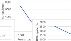
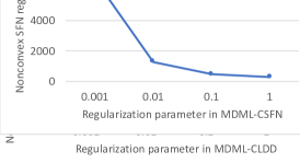
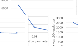
Figure 1: (Left) Nonconvex SFN regularizer versus the regularization parameter in MDML-CSFN; (Middle) Nonconvex LDD regularizer versus the regularization parameter in MDML-CLDD; (Right) Nonconvex VND regularizer versus the regularization parameter in MDML-CVND.

Additional experimental analysis

• Training time Unregularized PDML runs faster that regularized PDML methods because it has no need to tune the regularization parameter, which reduces the number of experimental runs by 4 times. Unregularized MDML runs faster than regularized MDML methods because it has no need to tune the regularization parameter or the number of projection vectors, which reduces the number of experimental runs by 12 times. PDML-(DC,DPP,VND,LDD) takes longer time than other regularized PDML methods since they need eigendecomposition to compute the gradients. PDML-OC has no regularization parameter to tune, hence its number of experimental runs is 4 times fewer than other regularized PDML methods.

• Balancedness In most DML methods, the AUC on infrequent classes is worse than that on frequent classes, showing that DML is sensitive to the imbalance of pattern-frequency, tends to be biased towards frequent patterns and is less capable to capture infrequent patterns. This is in accordance with previous study [56].

References

- [1] Davide Anguita, Alessandro Ghio, Luca Oneto, Xavier Parra, and Jorge L Reyes-Ortiz. Human activity recognition on smartphones using a multiclass hardware-friendly support vector machine. In Ambient assisted living and home care. Springer, 2012.
- [2] Robert E Banfield, Lawrence O Hall, Kevin W Bowyer, and W Philip Kegelmeyer. Ensemble diversity measures and their application to thinning. Information Fusion, 2005.
- [3] Yebo Bao, Hui Jiang, Lirong Dai, and Cong Liu. Incoherent training of deep neural networks to decorrelate bottleneck features for speech recognition. In 2013 IEEE International Conference on Acoustics, Speech and Signal Processing, 2013.
- [4] Peter L Bartlett and Shahar Mendelson. Rademacher and gaussian complexities: Risk bounds and structural results. Journal of Machine Learning Research, 3:463–482, 2003.
- [5] Aurélien Bellet and Amaury Habrard. Robustness and generalization for metric learning. Neurocomputing, 2015.
- [6] Stephen Boyd and Lieven Vandenberghe. Convex optimization. Cambridge university press, 2004.
- [7] Emmanuel Candes and Benjamin Recht. Exact matrix completion via convex optimization. Communications of the ACM, 55(6):111–119, 2012.
- [8] Miguel A Carreira-Perpinán and Ramin Raziperchikolaei. An ensemble diversity approach to supervised binary hashing. In Advances in Neural Information Processing Systems, pages 757–765, 2016.
- [9] Yong Chen, Hui Zhang, Yongxin Tong, and Ming Lu. Diversity regularized latent semantic match for hashing. Neurocomputing, 230:77–87, 2017.
- [10] Michael Cogswell, Faruk Ahmed, Ross Girshick, Larry Zitnick, and Dhruv Batra. Reducing overfitting in deep networks by decorrelating representations. ICLR, 2015.
- [11] Jason V Davis, Brian Kulis, Prateek Jain, Suvrit Sra, and Inderjit S Dhillon. Information-theoretic metric learning. In Proceedings of the 24th international conference on Machine learning. ACM, 2007.
- [12] Jia Deng, Wei Dong, Richard Socher, Li-Jia Li, Kai Li, and Li Fei-Fei. Imagenet: A large-scale hierarchical image database. In Computer Vision and Pattern Recognition, 2009. CVPR 2009. IEEE Conference on, pages 248–255. IEEE, 2009.
- [13] Xiping Fu, Brendan McCane, Steven Mills, and Michael Albert. Nokmeans: Non-orthogonal k-means hashing. In Asian Conference on Computer Vision, pages 162–177. Springer, 2014.
- [14] Mikel Galar, Alberto Fernandez, Edurne Barrenechea, Humberto Bustince, and Francisco Herrera. A review on ensembles for the class imbalance problem: bagging-, boosting-, and hybrid-based approaches. IEEE Transactions on Systems, Man, and Cybernetics, Part C (Applications and Reviews), 42(4):463–484, 2012.
- [15] Tiezheng Ge, Kaiming He, Qifa Ke, and Jian Sun. Optimized product quantization. IEEE transactions on pattern analysis and machine intelligence, 36(4):744–755, 2014.
- [16] Tiezheng Ge, Kaiming He, and Jian Sun. Graph cuts for supervised binary coding. In European Conference on Computer Vision, pages 250–264. Springer, 2014.
- [17] Ary L Goldberger, Luis AN Amaral, Leon Glass, Jeffrey M Hausdorff, Plamen Ch Ivanov, Roger G Mark, Joseph E Mietus, George B Moody, Chung-Kang Peng, and H Eugene Stanley. Physiobank, physiotoolkit, and physionet. Circulation, 101(23):e215–e220, 2000.
- [18] Yunchao Gong, Svetlana Lazebnik, Albert Gordo, and Florent Perronnin. Iterative quantization: A procrustean approach to learning binary codes for large-scale image retrieval. IEEE Transactions on Pattern Analysis and Machine Intelligence, 35(12):2916–2929, 2013.
- [19] Rudolf Gorenflo, Yuri Luchko, and Francesco Mainardi. Analytical properties and applications of the wright function. arXiv preprint math-ph/0701069, 2007.
- [20] Matthieu Guillaumin, Jakob Verbeek, and Cordelia Schmid. Is that you? metric learning approaches for face identification. In IEEE International Conference on Computer Vision. IEEE, 2009.
- [21] Amin Jalali, Lin Xiao, and Maryam Fazel. Variational gram functions: Convex analysis and optimization. arXiv preprint arXiv:1507.04734, 2015.
- [22] Jianqiu Ji, Shuicheng Yan, Jianmin Li, Guangyu Gao, Qi Tian, and Bo Zhang. Batch-orthogonal locality-sensitive hashing for angular similarity. IEEE transactions on pattern analysis and machine intelligence, 36(10):1963–1974, 2014.
- [23] Alistair EW Johnson, Tom J Pollard, Lu Shen, Li-wei H Lehman, Mengling Feng, Mohammad Ghassemi, Benjamin Moody, Peter Szolovits, Leo Anthony Celi, and Roger G Mark. Mimic-iii, a freely accessible critical care database. Scientific data, 3, 2016.
- [24] Weihao Kong and Wu-Jun Li. Isotropic hashing. In Advances in Neural Information Processing Systems, pages 1646–1654, 2012.
- [25] M Kostinger, Martin Hirzer, Paul Wohlhart, Peter M Roth, and Horst Bischof. Large scale metric learning from equivalence constraints. In IEEE Conference on Computer Vision and Pattern Recognition. IEEE, 2012.
- [26] Jonathan Krause, Michael Stark, Jia Deng, and Li Fei-Fei. 3d object representations for fine-grained categorization. In Proceedings of the IEEE International Conference on Computer Vision Workshops, pages 554–561, 2013.
- [27] Alex Kulesza, Ben Taskar, et al. Determinantal point processes for machine learning. Foundations and Trends® in Machine Learning, 5(2–3):123–286, 2012.
- [28] Brian Kulis et al. Metric learning: A survey. Foundations and Trends® in Machine Learning, 5(4):287–364, 2013.
- [29] Brian Kulis, Mátyás A Sustik, and Inderjit S Dhillon. Low-rank kernel learning with bregman matrix divergences. Journal of Machine Learning Research, 10(Feb):341–376, 2009.
- [30] Ludmila I Kuncheva and Christopher J Whitaker. Measures of diversity in classifier ensembles and their relationship with the ensemble accuracy. Machine learning, 2003.
- [31] Wei Liu, Steven Hoi, and Jianzhuang Liu. Output regularized metric learning with side information. Computer Vision–ECCV 2008, pages 358–371, 2008.
- [32] Wei Liu, Cun Mu, Rongrong Ji, Shiqian Ma, John R Smith, and Shih-Fu Chang. Low-rank similarity metric learning in high dimensions. In AAAI, pages 2792–2799, 2015.
- [33] Jonathan Malkin and Jeff Bilmes. Ratio semi-definite classifiers. In 2008 IEEE International Conference on Acoustics, Speech and Signal Processing, pages 4113–4116. IEEE, 2008.
- [34] Christopher D Manning, Prabhakar Raghavan, Hinrich Schütze, et al. Introduction to information retrieval, volume 1. Cambridge university press Cambridge, 2008.
- [35] Tomas Mikolov, Ilya Sutskever, Kai Chen, Greg S Corrado, and Jeff Dean. Distributed representations of words and phrases and their compositionality. In Advances in neural information processing systems, pages 3111–3119, 2013.
- [36] Michael A Nielsen and Isaac L Chuang. Quantum computation and Quantum information. 2000.
- [37] Gang Niu, Bo Dai, Makoto Yamada, and Masashi Sugiyama. Information-theoretic semisupervised metric learning via entropy regularization. Neural Computation, 2012.
- [38] Neal Parikh and Stephen Boyd. Proximal algorithms. Foundations and Trends in Optimization, 1(3):127–239, 2014.
- [39] Ioannis Partalas, Grigorios Tsoumakas, and Ioannis P Vlahavas. Focused ensemble selection: A diversity-based method for greedy ensemble selection. In European Conference on Artificial Intelligence, 2008.
- [40] Guo-Jun Qi, Jinhui Tang, Zheng-Jun Zha, Tat-Seng Chua, and Hong-Jiang Zhang. An efficient sparse metric learning in high-dimensional space via l1-penalized log-determinant regularization. In Proceedings of the 26th Annual International Conference on Machine Learning. ACM, 2009.
- [41] Qi Qian, Juhua Hu, Rong Jin, Jian Pei, and Shenghuo Zhu. Distance metric learning using dropout: a structured regularization approach. In Proceedings of the 20th ACM SIGKDD international conference on Knowledge discovery and data mining. ACM, 2014.
- [42] Ramin Raziperchikolaei and Miguel A Carreira-Perpinán. Learning independent, diverse binary hash functions: Pruning and locality. ICDM, 2016.
- [43] Karen Simonyan and Andrew Zisserman. Very deep convolutional networks for large-scale image recognition. arXiv preprint arXiv:1409.1556, 2014.
- [44] Nathan Srebro and Adi Shraibman. Rank, trace-norm and max-norm. In International Conference on Computational Learning Theory, pages 545–560. Springer, 2005.
- [45] Nitish Srivastava, Geoffrey E Hinton, Alex Krizhevsky, Ilya Sutskever, and Ruslan Salakhutdinov. Dropout: a simple way to prevent neural networks from overfitting. Journal of Machine Learning Research, 15(1):1929–1958, 2014.
- [46] Koji Tsuda, Gunnar Rätsch, and Manfred K Warmuth. Matrix exponentiated gradient updates for on-line learning and bregman projection. Journal of Machine Learning Research, 6(Jun):995–1018, 2005.
- [47] Nakul Verma and Kristin Branson. Sample complexity of learning mahalanobis distance metrics. arXiv preprint arXiv:1505.02729, 2015.
- [48] Daixin Wang, Peng Cui, Mingdong Ou, and Wenwu Zhu. Deep multimodal hashing with orthogonal regularization. In IJCAI, 2015.
- [49] Fei Wang and Jimeng Sun. Survey on distance metric learning and dimensionality reduction in data mining. Data Mining and Knowledge Discovery, 29(2):534–564, 2015.
- [50] Jun Wang, Sanjiv Kumar, and Shih-Fu Chang. Semi-supervised hashing for large-scale search. IEEE Transactions on Pattern Analysis and Machine Intelligence, 34(12):2393–2406, 2012.
- [51] Kilian Q Weinberger, John Blitzer, and Lawrence K Saul. Distance metric learning for large margin nearest neighbor classification. In Advances in neural information processing systems, 2005.
- [52] Yair Weiss, Antonio Torralba, and Rob Fergus. Spectral hashing. In Advances in neural information processing systems, pages 1753–1760, 2009.
- [53] Peter Welinder, Steve Branson, Takeshi Mita, Catherine Wah, Florian Schroff, Serge Belongie, and Pietro Perona. Caltech-ucsd birds 200. 2010.
- [54] Zaiwen Wen and Wotao Yin. A feasible method for optimization with orthogonality constraints. Mathematical Programming, 142(1-2):397–434, 2013.
- [55] Pengtao Xie. Learning compact and effective distance metrics with diversity regularization. In European Conference on Machine Learning, 2015.
- [56] Pengtao Xie, Yuntian Deng, and Eric P. Xing. Diversifying restricted boltzmann machine for document modeling. In ACM SIGKDD Conference on Knowledge Discovery and Data Mining, 2015.
- [57] Pengtao Xie, Barnabas Poczos, and Eric P Xing. Near-orthogonality regularization in kernel methods. 2017.
- [58] Eric P Xing, Michael I Jordan, Stuart Russell, and Andrew Y Ng. Distance metric learning with application to clustering with side-information. In Advances in neural information processing systems, 2002.
- [59] Wenbin Yao, Zhenyu Weng, and Yuesheng Zhu. Diversity regularized metric learning for person re-identification. In Image Processing (ICIP), 2016 IEEE International Conference on, pages 4264–4268. IEEE, 2016.
- [60] Yiming Ying, Kaizhu Huang, and Colin Campbell. Sparse metric learning via smooth optimization. In Advances in neural information processing systems, 2009.
- [61] Yiming Ying and Peng Li. Distance metric learning with eigenvalue optimization. The Journal of Machine Learning Research, 2012.
- [62] Yang Yu, Yu-Feng Li, and Zhi-Hua Zhou. Diversity regularized machine. In International Joint Conference on Artificial Intelligence. Citeseer, 2011.
- [63] Pourya Habib Zadeh, Reshad Hosseini, and Suvrit Sra. Geometric mean metric learning. In International Conference on Machine Learning, 2016.
- [64] Dengyong Zhou, Lin Xiao, and Mingrui Wu. Hierarchical classification via orthogonal transfer. ICML, 2011.
- [65] James Y Zou and Ryan P Adams. Priors for diversity in generative latent variable models. In Advances in Neural Information Processing Systems, pages 2996–3004, 2012.