Weak solutions for multiquasilinear elliptic-parabolic systems. Application to thermoelectrochemical problems

Abstract.

This paper investigates the existence of weak solutions of biquasilinear boundary value problem for a coupled elliptic-parabolic system of divergence form with discontinuous leading coefficients. The mathematical framework addressed in the article considers the presence of an additional nonlinearity in the model which reflects the radiative thermal boundary effects in some applications of interest. The results are obtained via the Rothe-Galerkin method. Only weak assumptions are made on the data and the boundary conditions are allowed to be on a general form. The major contribution of the current paper is the explicit expressions for the constants appeared in the quantitative estimates that are derived. These detailed and explicit estimates may be useful for the study on nonlinear problems that appear in the real world applications. In particular, they clarify the smallness conditions. In conclusion, we illustrate how the above results may be applied to the thermoelectrochemical phenomena in an electrolysis cell. This problem has several applications as for instance to optimize the cell design and operating conditions.

1. Introduction

The main gap between theory and practice is the unrealistic assumptions that are usually made by the mathematicians because they work in their theoretical results. Among them, they are the constant coefficients of the time derivative term in parabolic equations, or its independence on the space variable (commonly the density). In the real world applications, there are three terms that destroy the regularity of the solutions. The first quasilinear term classically stands for the spatial gradient of the solution, second one stands for the time derivative, and the third one appears from the power-type boundary condition. This power-type boundary condition represents the radiative heat transfer existent on a part of boundary. We mention to [25] for the transient radiative heat transfer equations in the one-dimensional slab.

Quantitative estimates take the characteristics of the coefficients into account, but usually include constants that hide some intrinsic characteristics of the domain. We seek for the complete explicitness of the constants that are involved on the quantitative estimates, and their effectiveness. We emphasize that their sharpness remains as an open problem. The main purpose is the analysis of a weak formulation of the corresponding boundary- and initial-value elliptic-parabolic problem. To that aim, we approximate the problem via implicit time discretization, by the classical Rothe method.

We point out that, in addition to the fact that Galerkin and Rothe methods are convenient tools for the theoretical analysis of elliptic and evolution problems [3, 11, 19, 29], it is of particular interest from the numerical point of view [16, 21, 23]. Different versions of the primal discontinuous Galerkin methods to treat the coupling of flow and transport and the coupling of transport and reaction have recently gained popularity because they are easier to implement than most traditional finite element methods, from a computer science point of view (see [30] and the references therein). Lipschitz continuity property is commonly assumed as a data character, which simplifies the Rothe method [13, 28].

The paper [9] deals with modeling of quasilinear thermoelectric phenomena, including the Peltier and Seebeck effects. In [5], the spatial distribution of the variables such as the electrolyte temperature, which is subject to local cell conditions, is studied. To optimize cell operations is the aim for the long term sustainability of the aluminum smelting industry.

The mathematical modeling of electrochemical devices such as Lithium-ion battery system [15, 22] has gaining of interest in the literature [26, 27, 33]. Here, no internal interfaces are considered in the model, which amounts to neglecting possible material heterogeneities as done in [6, 7, 8]. These works deal with weak solutions related to thermoelectrochemical devices with radiative effects in a part of the boundary, involving the cross effects. A particular feature is the mixture of some kind of (nonlinear) Neumann and Robin boundary conditions. Also, quantitative estimates are stated for the norm (steady-state in [6] and unsteady-state in [7]) under appropriate assumptions on the data, where the constants are given explicitly. Within this state of mind, we close this paper by applying the theoretical coupled elliptic-parabolic system to the thermoelectrochemical phenomena.

The structure of the paper is as follows. We begin by introducing the functional framework, the data under consideration and the main theorem in Section 2. The main ingredient of the proof is the Rothe method presented in Section 3. Section 4 deals to the existence proof of the corresponding elliptic problem. The idea of the proof is based on classical Galerkin approximation argument (Subsection 4.1). In Section 5, we derive a priori estimates for the approximate problem, getting compactness properties that allow the existence proof of the main theorem via the passage to the limit as the time-step vanishes. As a consequence of the main theoretical result, the existence of a weak solution to a thermoelectrochemical problem is stated in Section 6.

2. Introduction

Let $[0,T]\subset{\mathbb{R}}$ be the time interval with $T>0$ being an arbitrary (but preassigned) time. Let $\Omega$ be a bounded domain (that is, connected open set) in $\mathbb{R}^{n}$ ($n\geq 2$). Its boundary $\partial\Omega$ is constituted by three pairwise disjoint open $(n-1)$-dimensional sets, namely the electrodes surface $\Gamma$, the wall surface $\Gamma_{\mathrm{w}}$, and the remaining outer surface $\Gamma_{\mathrm{o}}$, such that $\partial\Omega=\overline{\Gamma}\cup\overline{\Gamma}_{\mathrm{w}}\cup\overline{\Gamma}_{\mathrm{o}}$. Observe that the electrodes surface $\Gamma$ consists of the anode $\Gamma_{\mathrm{a}}$ and the cathode $\Gamma_{\mathrm{c}}$. Figure 1 displays two schematic geometrical representations of the domain $\Omega$ and of its boundary $\partial\Omega$ in order to identify the various subsets into which the boundary is decomposed and, as a consequence, to better understand the physical significance of the enforced boundary conditions. Hence further, we set $Q_{T}=\Omega\times]0,T[$ and $\Sigma_{T}=\partial\Omega\times]0,T[$.

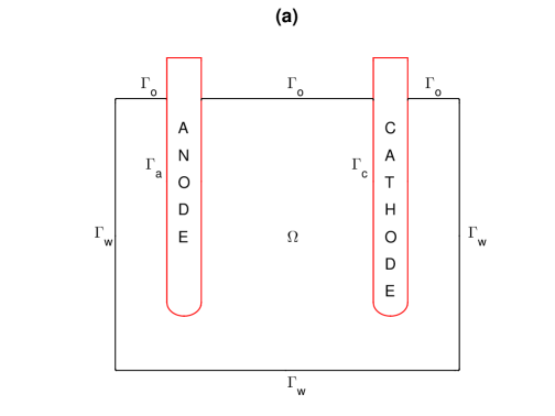
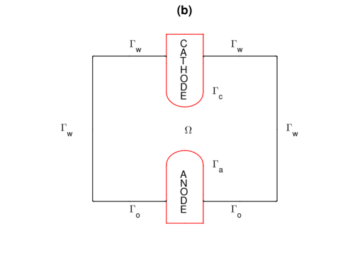
Figure 1. Schematic 2D representation of two cells of one compartment (not in scale). (a) an electrolytic cell. (b) TEC device design: heating bottom plate and two electrodes symmetrically placed [18].

We are interested in the following boundary value problem in the sense of distributions. Find the functions $(\mathbf{u},\phi):Q_{T}\rightarrow\mathbb{R}^{\mathrm{I}+2}$, with $\mathrm{I}$ being an integer number, that solve

$$\mathsf{B}(u_{\mathrm{I}+1})\partial_{t}\mathbf{u}-\nabla\cdot\left(\mathsf{A}(\mathbf{u})\nabla\mathbf{u}\right)=\nabla\cdot(\mathbf{F}(\mathbf{u})\nabla\phi);$$ (1)

$$-\nabla\cdot(\sigma(\mathbf{u})\nabla\phi)=\nabla\cdot(\mathbf{G}(\mathbf{u})\nabla\mathbf{u}) \mbox{ in }Q_{T},$$ (2)

with the following meaning of notation, for $j=1,\cdots,\mathrm{I}+1$,

$$\nabla\cdot\left(\mathsf{A}\nabla\mathbf{u}\right) = \sum_{k=1}^{n}\partial_{k}\left(\sum_{l=1}^{\mathrm{I}+1}a_{j,l}\partial_{k}u_{l}\right);$$

$$\nabla\cdot(F_{j}\nabla\phi) = \sum_{k=1}^{n}\partial_{k}(F_{j}\partial_{k}\phi);$$

$$\nabla\cdot(\mathbf{G}\nabla\mathbf{u}) = \sum_{k=1}^{n}\partial_{k}\left(\sum_{l=1}^{\mathrm{I}+1}G_{l}(\mathbf{u})\partial_{k}u_{l}\right).$$

Here $\mathsf{A}$ and $\mathsf{B}$ are $(\mathrm{I}+1)^{2}$-matrices such that

(A):

the leading matrix $\mathsf{A}$ is supposed to be uniformly elliptic, of quadratic-growth, and with real-valued $L^{\infty}$ components;

(B):

$\mathsf{B}$ is the diagonal matrix with non-zero components

$$b_{j,j}=\left\{\begin{array}[]{ll}1&\mbox{if }1\leq j\leq\mathrm{I}\\ b&\mbox{if }j=\mathrm{I}+1.\end{array}\right.$$

Only $(\mathrm{I}+1)$ parabolic equation is in fact known as the doubly nonlinear elliptic-parabolic equation which has been investigated by several authors when Dirichlet conditions are taken into account on the boundary (we refer for example to the works [4, 28] and the references cited therein for some details).

The Kirchoff transformation could be applied to the $(\mathrm{I}+1)$ parabolic equation in order to be useful in the time discretization because

$$b(u)\partial_{t}u=\partial_{t}\left(\int^{u}b(z)\mathrm{dz}\right),$$ (3)

although it is not truly useful as change variable because the function $b$ depends on the space variable and $\nabla\left(\int^{u}b(r)\mathrm{dr}\right)$ may be ill-defined.

The boundary conditions are in the concise form

$$\left(\mathsf{A}(\mathbf{u})\nabla\mathbf{u}+\mathbf{F}(\mathbf{u})\nabla\phi\right)\cdot\mathbf{n}+\mathbf{b}(u_{\mathrm{I}+1})^{\top}\mathbf{u}=\mathbf{h};$$ (4)

$$\left(\sigma(\mathbf{u})\nabla\phi+\mathbf{G}(\mathbf{u})\nabla\mathbf{u}\right)\cdot{\bf n}=g\chi_{\Gamma} \mbox{ on }\Sigma_{T},$$ (5)

with $\bf n$ denoting the outward unit normal to the boundary $\partial\Omega$, and

$$b_{j}=\left\{\begin{array}[]{ll}0&\mbox{if }1\leq j\leq\mathrm{I}\\ \gamma&\mbox{if }j=\mathrm{I}+1.\end{array}\right.$$

Here, the boundary coefficient $\gamma$ stands for the Robin-type boundary effects on $\Gamma$, and for the power-type boundary effects on $\Gamma_{\mathrm{w}}$. The functions $\mathbf{h}$ and $g$ stand for the boundary sources.

Finally, let the initial condition be

$$\mathbf{u}(\cdot,0)=\mathbf{u}^{0}\mbox{ in }\Omega.$$ (7)

In the framework of Sobolev and Lebesgue functional spaces, we use the following spaces of test functions:

$$V(\Omega) = \{v\in H^{1}(\Omega):\ \int_{\Omega}v\mathrm{dx}=0\};$$

$$V(\partial\Omega) = \{v\in H^{1}(\Omega):\ \int_{\partial\Omega}v\mathrm{ds}=0\};$$

$$V_{\ell}(\Omega) = \{v\in H^{1}(\Omega):\ v|_{\Gamma_{\mathrm{w}}}\in L^{\ell}(\Gamma_{\mathrm{w}})\};$$

$$V_{\ell}(Q_{T}) = \{v\in L^{2}(0,T;H^{1}(\Omega)):\ v|_{\Gamma_{\mathrm{w}}\times]0,T[}\in L^{\ell}(\Gamma_{\mathrm{w}}\times]0,T[)\},$$

with their usual norms, $\ell>1$. Hereafter, we use the notation ”ds” for the surface element in the integrals on the boundary as well as any subpart of the boundary $\partial\Omega$. Notice that $V_{\ell}(\Omega)\equiv H^{1}(\Omega)$ if $\ell<2_{*}$, where $2_{*}$ is the critical trace continuity constant, i.e. $2_{*}=2(n-1)/(n-2)$ if $n>2$ and $2_{*}>1$ is arbitrary if $n=2$.

The problem (1)-(2) is in fact a system of $\mathrm{I}+2$ partial differential equations and it may be decomposed in one system of $\mathrm{I}$ parabolic equations, one parabolic equation with a quasilinear time derivative, and one third elliptic equation.

Definition 2.1.

We say that a function $(\mathbf{u},\phi)$ is a weak solution to the problem (1)-(2) and (4)-(7), if it satisfies (7) and the variational formulation, with $u=u_{\mathrm{I}+1}$,

$$\int^{T}_{0}\langle\partial_{t}u_{i},v_{i}\rangle\mathrm{dt}+\sum_{j=1}^{\mathrm{I}+1}\int_{Q_{T}}a_{i,j}(\mathbf{u})\nabla u_{j}\cdot\nabla v_{i}\mathrm{dxdt}=$$

$$=-\int_{Q_{T}}F_{i}(\mathbf{u})\nabla\phi\cdot\nabla v_{i}\mathrm{dxdt}+\int_{\Sigma_{T}}h_{i}v_{i}\mathrm{dsdt},\quad i=1,\cdots,\mathrm{I};$$ (8)

$$\int^{T}_{0}\langle b(u)\partial_{t}u,v\rangle\mathrm{dt}+\sum_{j=1}^{\mathrm{I}+1}\int_{Q_{T}}a_{\mathrm{I}+1,j}(\mathbf{u})\nabla u_{j}\cdot\nabla v\mathrm{dxdt}+\int_{\Sigma_{T}}\gamma(u)uv\mathrm{dsdt}=$$

$$=-\int_{Q_{T}}F_{\mathrm{I}+1}(\mathbf{u})\nabla\phi\cdot\nabla v\mathrm{dxdt}+\int_{\Sigma_{T}}h_{\mathrm{I}+1}v\mathrm{dsdt};\qquad$$ (9)

$$\int_{\Omega}\sigma(\mathbf{u})\nabla\phi\cdot\nabla w\mathrm{dx}=-\sum_{j=1}^{\mathrm{I}+1}\int_{\Omega}G_{j}(\mathbf{u})\nabla u_{j}\cdot\nabla w\mathrm{dx}+\int_{\Gamma}gw\mathrm{ds},\ \mbox{a.e. in }]0,T[,$$ (10)

for all $v_{i}\in L^{2}(0,T;V(\Omega))$, $v\in V_{\ell}(Q_{T})$, and $w\in V(\partial\Omega)$.

The symbol $\langle\cdot,\cdot\rangle$ denotes the duality pairing $\langle\cdot,\cdot\rangle_{X^{\prime}\times X}$, with $X$ being a Banach space. The notation $X^{\prime}$ denotes the dual space of $X$, and $X^{\prime}$ is equipped with the usual induced norm $\|f\|_{X^{\prime}}=\sup\{\langle f,u\rangle,\ u\in X:\|u\|_{X}\leq 1\}$.

The set of hypothesis is as follows.

(H1):

The vector-valued functions $\mathbf{F}$ and $\mathbf{G}$, from $\Omega\times\mathbb{R}^{\mathrm{I}+1}$ into $\mathbb{R}^{\mathrm{I}+1}$, are assumed to be Carathéodory, i.e. measurable with respect to $x\in\Omega$ and continuous with respect to other variables, such that verify

$$\exists F_{j}^{\#}>0: |F_{j}(x,\mathbf{e})|\leq F_{j}^{\#};$$ (11)

$$\exists G_{j}^{\#}>0: |G_{j}(x,\mathbf{e})|\leq G_{j}^{\#},$$ (12)

for all $j=1,\cdots,\mathrm{I}+1$, for a.e. $x\in\Omega$, and for all $\mathbf{e}\in\mathbb{R}^{\mathrm{I}+1}$.

(H2):

The coefficient $b$ is assumed to be a Carathéodory function from $\Omega\times\mathbb{R}$ into $\mathbb{R}$. Moreover, there exist $b_{\#},b^{\#}>0$ such that

$$b_{\#}\leq b(x,e)\leq b^{\#},$$ (13)

for a.e. $x\in\Omega$, and for all $e\in\mathbb{R}$.

(H3):

The leading coefficient $\mathsf{A}$ has its components $a_{i,j}:\Omega\times\mathbb{R}^{\mathrm{I}+1}\rightarrow\mathbb{R}$ being Carathéodory functions. Moreover, they satisfy

$$(a_{i})_{\#}:=\min_{(x,\mathbf{e})\in\Omega\times\mathbb{R}^{\mathrm{I}+1}}a_{i,i}(x,\mathbf{e})>0;$$ (14)

$$\exists a_{i,j}^{\#}>0:\quad|a_{i,j}(\cdot,\mathbf{e})|\leq a_{i,j}^{\#},\quad\mbox{a.e. in }\Omega,\ \forall\mathbf{e}\in\mathbb{R}^{\mathrm{I}+1},$$ (15)

for all $i,j\in\{1,\cdots,\mathrm{I}+1\}$.

(H4):

The leading coefficient $\sigma$ is assumed to be a Carathéodory function from $\Omega\times\mathbb{R}^{\mathrm{I}+1}$ into $\mathbb{R}$. Moreover, there exist $\sigma_{\#},\sigma^{\#}>0$ such that

$$\sigma_{\#}\leq\sigma(x,\mathbf{e})\leq\sigma^{\#},$$ (16)

for a.e. $x\in\Omega$, and for all $\mathbf{e}\in\mathbb{R}^{\mathrm{I}+1}$.

(H5):

The boundary coefficient $\gamma$ is assumed to be a Carathéodory function from $\partial\Omega\times\mathbb{R}$ into $\mathbb{R}$. Moreover, there exist $\gamma_{\#},\gamma^{\#}>0$ and $\gamma_{1}\geq 0$ such that

$$\gamma_{\#}|e|^{\ell-2}\leq\gamma(\cdot,e)\leq\gamma^{\#}|e|^{\ell-2}+\gamma_{1},$$ (17)

a.e. in $\partial\Omega$, and for all $e\in\mathbb{R}$, where the exponent $\ell\geq 2$ stands for the Robin-type boundary condition ($\ell=2$) on $\Gamma$, and for the power-type boundary condition ($\ell>2$) on $\Gamma_{\mathrm{w}}$.

Remark 2.1.

The boundary condition (17) may be generalized for a function $\gamma_{1}:\partial\Omega\rightarrow\mathbb{R}$ belonging to $L^{\ell/(\ell-2)}(\partial\Omega)$ for $\ell\geq 2$. Indeed, Theorem 2.1 remains valid if (17) is replaced by

$$|\gamma(\cdot,e)|\leq\gamma_{1} \mbox{ a.e. on }\Gamma;$$

$$\gamma_{\#}|e|^{\ell-2}\leq\gamma(\cdot,e)\leq\gamma^{\#}|e|^{\ell-2}+\gamma_{1} \mbox{ a.e. on }\Gamma_{\mathrm{w}},$$

for all $e\in\mathbb{R}$, which infer in Section 4.1 that the Brouwer fixed point theorem is applied for a different $r>0$ taking Definition 4.1 into account.

Hereafter, we will use the Kirchoff transformation (3) to the time derivative term, i.e. the characterization $\partial_{t}B(u)$, denoting by $B$ the operator defined by

$$v\in L^{2}(Q_{T})\mapsto B(v)=\int_{0}^{v}b(\cdot,z)\mathrm{dz}.$$ (18)

Let us state the existence results.

Theorem 2.1.

Suppose that the assumptions (H1)-(H5), $h_{i}\in L^{2}(\Sigma_{T})$, $i=1,\cdots,\mathrm{I}$, $h_{\mathrm{I}+1}\in L^{\ell/(\ell-1)}(\Sigma_{T})$, and $g\in L^{2}(\Gamma)$ be fulfilled. Under the smallness conditions, for $i\in\{1,\cdots,\mathrm{I}+1\}$,

$$(a_{i})_{\#} > \frac{1}{2}\left(\sum_{l=1\atop l\not=i}^{\mathrm{I}+1}(a_{i,l}^{\#}+a_{l,i}^{\#})+F_{i}^{\#}+G_{i}^{\#}\right),$$ (19)

$$\sigma_{\#} > \frac{1}{2}\sum_{j=1}^{\mathrm{I}+1}\left(F_{j}^{\#}+G_{j}^{\#}\right),$$ (20)

there exists at least one weak solution $(\mathbf{u},\phi)\in[L^{\infty}(0,T;L^{2}(\Omega))]^{\mathrm{I}+1}\times L^{2}(0,T;V(\partial\Omega))$ in accordance to Definition 2.1, with $v\in L^{\ell}(0,T;V_{\ell}(\Omega))$, such that

$$u_{i}-u^{0}_{i}\in L^{2}(0,T;V(\Omega))\quad\mbox{and}\quad\partial_{t}u_{i}\in L^{2}(0,T;(V(\Omega))^{\prime});$$

$$u\in V_{\ell}(Q_{T})\quad\mbox{and}\quad b(u)\partial_{t}u\in L^{\ell^{\prime}}(0,T;(V_{\ell}(\Omega))^{\prime}),$$

for $i=1,\cdots,\mathrm{I}$. In particular, $B(u)\in L^{\infty}(0,T;L^{1}(\Omega))$.

Here, we consider the Banach spaces that are of direct application for the thermoelectrochemical problem under study. Clearly, Theorem 2.1 remains valid for any closed subspace $V$ such that $H^{1}_{0}(\Omega)\hookrightarrow V\hookrightarrow H^{1}(\Omega)$ is considered instead of $V(\Omega)$ or $V(\partial\Omega)$ if the Poincaré inequality is verified.

Remark 2.2.

In (8)-(9), the meaning of the time derivative should be understood as in the following weak sense [4]:

$$\int^{T}_{0}\langle\partial_{t}u_{i},v_{i}\rangle\mathrm{dt} = -\int^{T}_{0}\int_{\Omega}u_{i}\partial_{t}v_{i}\mathrm{dx}\mathrm{dt}-\int_{\Omega}u_{i}^{0}v_{i}(0)\mathrm{dx};$$ (21)

$$\int^{T}_{0}\langle b(u)\partial_{t}u,v\rangle\mathrm{dt} = -\int^{T}_{0}\int_{\Omega}B(u)\partial_{t}v\mathrm{dx}\mathrm{dt}-\int_{\Omega}B(u^{0})v(0)\mathrm{dx},$$ (22)

for every test functions $v_{i}\in L^{2}(0,T;V(\Omega))\cap W^{1,1}(0,T;L^{\infty}(\Omega))$, for $i\in\{1,\cdots,\mathrm{I}\}$, and $v\in L^{\ell}(0,T;V_{\ell}(\Omega))\cap W^{1,1}(0,T;L^{\infty}(\Omega))$ such that $v_{i}(T)=v(T)=0$ a.e. in $\Omega$.

3. Time discretization technique

We adopt the weak solvability of $\mathrm{I}+1$ time dependent partial differential equation with a nonlinear Neumann boundary condition as investigated in [4, 20], while the $j$ parabolic equations ($j=1,\cdots,\mathrm{I}$) are studied via the classical time discretization technique [19]. We introduce a recurrent system of boundary value problems to be successively solved for $m=1,\cdots,M\in\mathbb{N}$, starting from the initial function (7).

We decompose the time interval $I=[0,T]$ into $M$ subintervals $I_{m,M}$ of size $\tau$ (commonly called time step) such that $M=T/\tau\in\mathbb{N}$, i.e. $I_{m,M}=[(m-1)T/M,mT/M]$ for $m\in\{1,\cdot\cdot\cdot,M\}$. We set $t_{m,M}=mT/M$.

For any time integrable function $h:\Sigma_{T}\rightarrow\mathbb{R}$, we set

$$\bar{h}^{m}=\frac{1}{\tau}\int_{(m-1)\tau}^{m\tau}h(\cdot,z)\mathrm{dz}.$$ (23)

Then, the problem (8)-(10) is approximated by the following recurrent sequence of time discretized problems

$$\frac{1}{\tau}\int_{\Omega}u_{i}^{m}v_{i}\mathrm{dx}+\sum_{j=1}^{\mathrm{I}+1}\int_{\Omega}a_{i,j}(\mathbf{u}^{m})\nabla u_{j}^{m}\cdot\nabla v_{i}\mathrm{dx}+\int_{\Omega}F_{i}(\mathbf{u}^{m})\nabla\phi^{m}\cdot\nabla v_{i}\mathrm{dx}=$$

$$=\frac{1}{\tau}\int_{\Omega}u_{i}^{m-1}v_{i}\mathrm{dx}+\int_{\partial\Omega}\bar{h}^{m}_{i}v_{i}\mathrm{ds},\quad i=1,\cdots,\mathrm{I};\qquad$$ (24)

$$\frac{1}{\tau}\int_{\Omega}B(u^{m})v\mathrm{dx}+\sum_{j=1}^{\mathrm{I}+1}\int_{\Omega}a_{\mathrm{I}+1,j}(\mathbf{u}^{m})\nabla u_{j}^{m}\cdot\nabla v\mathrm{dx}+\int_{\Omega}F_{\mathrm{I}+1}(\mathbf{u}^{m})\nabla\phi^{m}\cdot\nabla v\mathrm{dx}+$$

$$+\int_{\partial\Omega}\gamma(u^{m})u^{m}v\mathrm{ds}=\frac{1}{\tau}\int_{\Omega}B(u^{m-1})v\mathrm{dx}+\int_{\partial\Omega}\bar{h}^{m}_{\mathrm{I}+1}v\mathrm{ds};\qquad$$ (25)

$$\int_{\Omega}\sigma(\mathbf{u}^{m})\nabla\phi^{m}\cdot\nabla w\mathrm{dx}+\sum_{j=1}^{\mathrm{I}+1}\int_{\Omega}G_{j}(\mathbf{u}^{m})\nabla u_{j}^{m}\cdot\nabla w\mathrm{dx}=\int_{\Gamma}gw\mathrm{ds},\qquad$$ (26)

where $\mathbf{u}=(u_{1},\cdots,u_{\mathrm{I}},u)$, for all $v_{i}\in V(\Omega)$, $i=1,\cdots,\mathrm{I}$, $v\in V_{\ell}(\Omega)$ and $w\in V(\partial\Omega)$. Since $\mathbf{u}^{0}\in L^{2}(\Omega)$ is known, we determine $\mathbf{u}^{1}$ as the unique solution of Proposition 3.1, and we inductively proceed.

The existence of the above system of elliptic problems is established in the following proposition.

Proposition 3.1.

Let $m\in\{1,\cdot\cdot\cdot,M\}$ be fixed, and $\mathbf{u}^{m-1}$ be given. Then, there exists a unique solution $(\mathbf{u}^{m},\phi^{m})\in[V(\Omega)]^{\mathrm{I}}\times V_{\ell}(\Omega)\times V(\partial\Omega)$ to the variational system (24)-(26).

This existence of solution is proved in Section 4 via the Galerkin method (cf. Subsection 4.1).

Let us recall the technical result [4, 20].

Lemma 3.1.

Denoting by

$$\Psi(s):=B(s)s-\int_{0}^{s}B(r)\mathrm{dr}=\int_{0}^{s}(B(s)-B(r))\mathrm{dr},$$

there holds

$$\int_{\Omega}(B(u)-B(v))u\mathrm{dx}\geq\int_{\Omega}\Psi(u)\mathrm{dx}-\int_{\Omega}\Psi(v)\mathrm{dx}.$$ (27)

In particular, if the assumption (13) is fulfilled then there holds

$$\int_{\Omega}\Psi(u)\mathrm{dx}\leq\int_{\Omega}B(u)u\mathrm{dx}\leq b^{\#}\|u\|_{2,\Omega}^{2}.$$

Under the assumption (13) the operator $B$ verifies

$$(B(u)-B(v),u-v)\geq b_{\#}\|u-v\|_{2,\Omega}^{2}.$$ (28)

In order to control the time dependence, we begin by recalling the following remarkable lemma [4, Lemma 1.9].

Lemma 3.2.

Suppose $u_{m}$ weakly converge to $u$ in $L^{p}(0,T;W^{1,p}(\Omega))$, $p>1$, with the estimates

$$\int_{\Omega}\Psi(u_{m}(t))\mathrm{dx}\leq C\quad\mbox{for }0<t<T,$$

and for $z>0$

$$\int_{0}^{T-z}\int_{\Omega}(B(u_{m}(t+z))-B(u_{m}(t)))(u_{m}(t+z)-u_{m}(t))\mathrm{dx}\mathrm{dt}\leq Cz,$$ (29)

with $C$ being positive constants. Then, $B(u_{m})\rightarrow B(u)$ in $L^{1}(Q_{T})$ and $\Psi(u_{m})\rightarrow\Psi(u)$ almost everywhere in $Q_{T}$.

In the sequel, we will also need both the discrete Gronwall inequality and the Aubin-Lions theorem. Let us recall the following discrete version of the Gronwall inequality [20].

Lemma 3.3 (Discrete Gronwall inequality).

Let $\{a_{m}\}_{m\in\mathbb{N}}$ and $\{A_{m}\}_{m\in\mathbb{N}}$ be sequences of nonnegative real numbers such that $A_{m}$ is nondecreasing and

$$a_{m}\leq A_{m}+\tau L\sum_{j=1}^{m}a_{j},$$

for each $m\in\mathbb{N}$ and for some $0<\tau L<1$. Then, there holds

$$a_{m}\leq\frac{A_{m}}{1-\tau L}\exp[(m-1)\tau].$$

Let us recall the following version of the Aubin-Lions theorem for piecewise constant functions [12].

Theorem 3.1 (Aubin-Lions).

Let $X$, $B$, and $Y$ be Banach spaces such that the embeddings $X\hookrightarrow\hookrightarrow B\hookrightarrow Y$ hold, and let $T>0$ and $1\leq p<\infty$. Let $\{u_{M}\}_{M\in\mathbb{N}}$ be a sequence of functions, which are constant on each time subinterval $](k-1)\tau,k\tau]$ with uniform time step $\tau=T/M$, satisfying

$$\tau^{-1}\|u_{M}-u_{M-1}\|_{L^{1}(\tau,T;Y)}+\|u_{M}\|_{L^{p}(0,T;X)}\leq C_{0},\quad\forall\tau>0,$$

where $C_{0}$ is a positive constant independent on $\tau$. Then, there exists a subsequence of $\{u_{M}\}_{M\in\mathbb{N}}$ strongly converging in $L^{p}(0,T;B)$.

4. Proof of Proposition 3.1

Let $m\in\{1,\cdot\cdot\cdot,M\}$ be fixed, and $\mathbf{u}^{m-1}$ be given. Set $\mathbf{f}=\mathbf{u}^{m-1}$, and $\mathbf{g}$ be such that

$$g_{j}=\left\{\begin{array}[]{ll}\bar{h}^{m}_{j}&\mbox{if }1\leq j\leq\mathrm{I}+1\\ g\chi_{\Gamma}&\mbox{if }j=\mathrm{I}+2.\end{array}\right.$$ (30)

Set the $(\mathrm{I}+2)^{2}$-matrix

$$\mathsf{L}(\mathbf{u})=\left[\begin{array}[]{cc}\mathsf{A}(\mathbf{u})&\mathbf{F}(\mathbf{u})\\ \mathbf{G}^{\top}(\mathbf{u})&\sigma(\mathbf{u})\end{array}\right].$$ (31)

Using the assumptions (11), (12) and (14)-(16) we find

$$\sum_{j,l=1}^{\mathrm{I}+2}\sum_{\iota=1}^{n}\left(L_{j,l}(\mathbf{u})\xi_{l,\iota}\right)\xi_{j,\iota}\geq\sum_{j=1}^{\mathrm{I}+2}\sum_{\iota=1}^{n}(L_{j})_{\#}|\xi_{j,\iota}|^{2},$$ (32)

where, for $j=1,\cdots,\mathrm{I}+1$,

$$(L_{j})_{\#} = (a_{j})_{\#}-\frac{1}{2}\left(\sum_{l=1\atop l\not=j}^{\mathrm{I}+1}(a_{l,j}^{\#}+a_{j,l}^{\#})+F_{j}^{\#}+G_{j}^{\#}\right);$$

$$(L_{\mathrm{I}+2})_{\#} = \sigma_{\#}-\frac{1}{2}\sum_{j=1}^{\mathrm{I}+1}\left(F_{j}^{\#}+G_{j}^{\#}\right).$$

Remark 4.1.

Although the positive-definiteness implies invertibility, there are invertible matrices that are not positive definite. The existence of the inverse matrix $\mathsf{L}^{-1}$ may be consequence of det$(\mathsf{L})\not=0$. An alternative sufficient condition is that rank$\left(\mathsf{L}\right)=\mathrm{I}+2$.

Definition 4.1.

We call by $K_{2}(P_{2}+1)$ the constant that verifies

$$\|v\|_{2,\Gamma}\leq K_{2}\left(\|v\|_{2,\Omega}+\|\nabla v\|_{2,\Omega}\right)\leq K_{2}(P_{2}+1)\|\nabla v\|_{2,\Omega},\quad\forall v\in H^{1}(\Omega).$$ (33)

Here, $K_{2}$ stands to the continuity constant of the trace embedding $H^{1}(\Omega)\hookrightarrow L^{2}(\Gamma)$, and $P_{2}$ stands to the Poincaré constant correspondent to the space exponent $2$.

4.1. Galerkin approximation technique

The Banach space $\mathbf{V}:=[V(\Omega)]^{\mathrm{I}}\times V_{\ell}(\Omega)\times V(\partial\Omega)$ admits linearly independent functions $\mathbf{w}^{\nu}$, $\nu=1,\cdots,N$, such that the finite-dimensional subspace $\mathbf{V}_{N}=\mathrm{span}\{\mathbf{w}^{1},\cdots,\mathbf{w}^{N}\}$ is dense in $\mathbf{V}$, for every $N\in{\mathbb{N}}$.

Introduce the continuous function $P:\mathbb{M}_{(\mathrm{I}+2)\times N}\rightarrow\mathbb{M}_{(\mathrm{I}+2)\times N}$ that maps $\left[\lambda_{j,\nu}\right]$ into $\left[\beta_{j,\nu}\right]$, defined by for each $\nu=1,\cdots,N$

$$\beta_{j,\nu} = \frac{1}{\tau}\int_{\Omega}U^{N}_{j}w_{j}^{\nu}\mathrm{dx}+\sum_{l=1}^{\mathrm{I}+2}\int_{\Omega}\left(L_{j,l}(\mathbf{U}^{N})\nabla U_{l}^{N}\right)\cdot\nabla w_{j}^{\nu}\mathrm{dx}$$

$$-\frac{1}{\tau}\int_{\Omega}f_{j}w_{j}^{\nu}\mathrm{dx}-\int_{\partial\Omega}g_{j}w_{j}^{\nu}\mathrm{ds},\quad\forall j=1,\cdots,\mathrm{I};$$

$$\beta_{j,\nu} = \frac{1}{\tau}\int_{\Omega}b(U^{N}_{\mathrm{I}+1})U^{N}_{j}w_{j}^{\nu}\mathrm{dx}+\sum_{l=1}^{\mathrm{I}+2}\int_{\Omega}\left(L_{j,l}(\mathbf{U}^{N})\nabla U_{l}^{N}\right)\cdot\nabla w_{j}^{\nu}\mathrm{dx}+$$

$$+\int_{\partial\Omega}\gamma(U^{N}_{\mathrm{I}+1})U^{N}_{j}w_{j}^{\nu}\mathrm{ds}-\frac{1}{\tau}\int_{\Omega}b(U^{N}_{\mathrm{I}+1})f_{j}w_{j}^{\nu}\mathrm{dx}-\int_{\partial\Omega}g_{j}w_{j}^{\nu}\mathrm{ds},\quad j=\mathrm{I}+1;$$

$$\beta_{j,\nu} = \sum_{l=1}^{\mathrm{I}+2}\int_{\Omega}\left(L_{j,l}(\mathbf{U}^{N})\nabla U_{l}^{N}\right)\cdot\nabla w_{j}^{\nu}\mathrm{dx}-\int_{\partial\Omega}g_{j}w_{j}^{\nu}\mathrm{ds},\quad j=\mathrm{I}+2,$$

with the function $\mathbf{U}^{N}\in\mathbf{V}_{N}$ being in the form

$$U_{j}^{N}(x)=\sum_{\nu=1}^{N}\lambda_{j,\nu}^{N}w_{j}^{\nu}(x),\quad j=1,\cdots,\mathrm{I}+2.$$

In order to apply the Brouwer fixed point theorem [24], we must prove that $P$ satisfies $(P\lambda,\lambda)>0$ for all $\lambda\in\mathbb{M}_{(\mathrm{I}+2)\times N}$ such that $|\lambda|=\left(\sum_{j=1}^{\mathrm{I}+1}\sum_{\nu=1}^{N}\lambda_{j,\nu}^{2}\right)^{1/2}=r$, and $(\beta,\lambda)$ stands for the inner product in $\mathbb{M}_{(\mathrm{I}+2)\times N}$. To this aim, we compute

$$(P\lambda,\lambda) = \sum_{j=1}^{\mathrm{I}+2}\sum_{\nu=1}^{N}\beta_{j,\nu}\lambda_{j,\nu}=$$

$$= \frac{1}{\tau}\sum_{j=1}^{\mathrm{I}+1}\int_{\Omega}b_{j,j}(U^{N}_{\mathrm{I}+1})|U^{N}_{j}|^{2}\mathrm{dx}+\sum_{j=1}^{\mathrm{I}+2}\sum_{l=1}^{\mathrm{I}+2}\int_{\Omega}\left(L_{j,l}(\mathbf{U}^{N})\nabla U_{l}^{N}\right)\cdot\nabla U_{j}^{N}\mathrm{dx}$$

$$+\int_{\partial\Omega}\gamma(U^{N}_{\mathrm{I}+1})|U^{N}_{\mathrm{I}+1}|^{2}\mathrm{ds}-\frac{1}{\tau}\sum_{j=1}^{\mathrm{I}+1}\int_{\Omega}b_{j,j}(U^{N}_{\mathrm{I}+1})f_{j}U_{j}^{N}\mathrm{dx}-\sum_{j=1}^{\mathrm{I}+2}\int_{\partial\Omega}g_{j}U_{j}^{N}\mathrm{ds}.$$

Applying the assumptions (13) and (17), the Hölder inequality, and (33), we obtain

$$(P\lambda,\lambda) \geq \frac{1}{\tau}\sum_{j=1}^{\mathrm{I}}\left(\|U^{N}_{j}\|_{2,\Omega}-\|f_{j}\|_{2,\Omega}-K_{2}\|g_{j}\|_{2,\partial\Omega}\right)\|U^{N}_{j}\|_{2,\Omega}+$$

$$+\frac{1}{\tau}\left(b_{\#}\|U^{N}_{\mathrm{I}+1}\|_{2,\Omega}-b^{\#}\|f_{\mathrm{I}+1}\|_{2,\Omega}\right)\|U_{\mathrm{I}+1}^{N}\|_{2,\Omega}+$$

$$+\sum_{j=1}^{\mathrm{I}}\left((L_{j})_{\#}\|\nabla U_{j}^{N}\|_{2,\Omega}-K_{2}\|g_{j}\|_{2,\partial\Omega}\right)\|\nabla U_{j}^{N}\|_{2,\Omega}+$$

$$+(L_{\mathrm{I}+1})_{\#}\|\nabla U_{\mathrm{I}+1}^{N}\|_{2,\Omega}^{2}+$$

$$+\left(\gamma_{\#}\|U^{N}_{\mathrm{I}+1}\|_{\ell,\partial\Omega}^{\ell-1}+\gamma_{1}\|U^{N}_{\mathrm{I}+1}\|_{\ell^{\prime},\partial\Omega}-\|g_{\mathrm{I}+1}\|_{\ell^{\prime},\partial\Omega}\right)\|U^{N}_{\mathrm{I}+1}\|_{\ell,\partial\Omega}+$$

$$+\left((L_{\mathrm{I}+2})_{\#}\|\nabla U_{\mathrm{I}+2}^{N}\|_{2,\Omega}-K_{2}(P_{2}+1)\|g_{\mathrm{I}+2}\|_{2,\partial\Omega}\right)\|\nabla U_{\mathrm{I}+2}^{N}\|_{2,\Omega}.$$

Then, there exists $r>0$ such that fulfills $(P\lambda,\lambda)>0$. We are in the position of applying the Brouwer fixed point theorem. Consequently, there exists $\lambda\in\mathbb{M}_{(\mathrm{I}+2)\times N}$ such that $|\lambda|\leq r$ and $P([\lambda_{j,\nu}])=0$, i.e. taking the density of $\mathbf{V}_{N}$ into $\mathbf{V}$,

$$\frac{1}{\tau}\sum_{j=1}^{\mathrm{I}}\int_{\Omega}U^{N}_{j}v_{j}\mathrm{dx}+\frac{1}{\tau}\int_{\Omega}b(U^{N}_{\mathrm{I}+1})U^{N}_{\mathrm{I}+1}v_{\mathrm{I}+1}\mathrm{dx}+$$

$$+\sum_{j=1}^{\mathrm{I}+2}\sum_{l=1}^{\mathrm{I}+2}\int_{\Omega}\left(L_{j,l}(\mathbf{U}^{N})\nabla U_{l}^{N}\right)\cdot\nabla v_{j}\mathrm{dx}+\int_{\partial\Omega}\gamma(U^{N}_{\mathrm{I}+1})U^{N}_{\mathrm{I}+1}v_{\mathrm{I}+1}\mathrm{ds}=$$

$$=\frac{1}{\tau}\sum_{j=1}^{\mathrm{I}}\int_{\Omega}f_{j}v_{j}\mathrm{dx}+\frac{1}{\tau}\int_{\Omega}b(U^{N}_{\mathrm{I}+1})f_{\mathrm{I}+1}v_{\mathrm{I}+1}\mathrm{dx}+\sum_{j=1}^{\mathrm{I}+2}\int_{\partial\Omega}g_{j}v_{j}\mathrm{ds}.$$ (34)

In order to pass to the limit in the variational equality (34) with $N$, when $N$ tends to infinity, we can extract a subsequence, still denoted by $\mathbf{U}^{N}$, convergent to $\mathbf{U}$ weakly in $\mathbf{V}$ and strongly in $\mathbf{L}^{2}(\Omega)$ and in $\mathbf{L}^{2}(\partial\Omega)$. In particular, $\mathbf{U}^{N}$ pointwisely converges to $\mathbf{U}$ a.e. in $\Omega$ and on $\partial\Omega$. Applying the Krasnoselski theorem to the Nemytskii operators $b$ and $\mathsf{L}$, we have

$$b(U^{N}_{\mathrm{I}+1})v\mathrel{\mathop{\kern 0.0pt\longrightarrow}\limits^{N\rightarrow\infty}}b(U_{\mathrm{I}+1})v L^{2}(\Omega);$$ in (35)

$$\sum_{j=1}^{\mathrm{I}+2}L_{j,l}(\mathbf{U}^{N})\nabla v_{j}\mathrel{\mathop{\kern 0.0pt\longrightarrow}\limits^{N\rightarrow\infty}}\sum_{j=1}^{\mathrm{I}+2}L_{j,l}(\mathbf{U})\nabla v_{j} \mathbf{L}^{2}(\Omega),$$ in (36)

for $l=1,\cdots,\mathrm{I}+1$, and for all $v,v_{j}\in H^{1}(\Omega)$, making use of the Lebesgue dominated convergence theorem with the assumptions (11)-(16). Similarly, the boundary term $\gamma(U^{N}_{\mathrm{I}+1})v$ converges to $\gamma(U_{\mathrm{I}+1})v$ in $L^{\ell^{\prime}}(\partial\Omega)$, for all $v\in L^{\ell^{\prime}}(\partial\Omega)$, due to (17). Thus, we are in the condition of passing to the limit in the variational equality (34) as $N$ tends to infinity to conclude that $\mathbf{U}$ is the required limit solution.

5. Passage to the limit as time goes to zero ($M\rightarrow+\infty$)

Set $\mathbf{X}_{\ell}=[V(\Omega)]^{\mathrm{I}}\times V_{\ell}(\Omega)$. Let $\widetilde{\mathbf{u}}^{M}:]0,T[\rightarrow\mathbf{X}_{\ell}$ and $\widetilde{\phi}^{M}:]0,T[\rightarrow V(\partial\Omega)$ be the step functions defined by

$$\widetilde{\mathbf{u}}^{M}(t)=\left\{\begin{array}[]{ll}\mathbf{u}^{0}&\mbox{ if }t=0\\ \mathbf{u}^{m}&\mbox{ if }t\in]t_{m-1,M},t_{m,M}]\end{array}\right.$$ (39)

$$\widetilde{\phi}^{M}(t)=\phi^{m}\quad\mbox{ if }t\in]t_{m-1,M},t_{m,M}],$$ (40)

and let $h^{M}\in L^{\infty}(0,T;L^{1}(\partial\Omega))$ be the (piecewise constant in time) function given by $h^{M}(t)=\bar{h}^{m}$ for $t\in](m-1)\tau,m\tau]$ (cf. (23)).

We begin by establishing the estimates and the weak convergences of the Rothe function

$$(\widetilde{\mathbf{u}}^{M},\widetilde{\phi}^{M})=(\widetilde{u}_{1}^{M},\cdots,\widetilde{u}_{\mathrm{I}}^{M},\widetilde{u}^{M},\widetilde{\phi}^{M})$$

obtained from the discretized solution $({\mathbf{u}}^{m},\phi^{m})$, of variational system (24)-(26), by piecewise constant interpolation with respect to time $t$.

Proposition 5.1.

Denoting by $\{(\widetilde{\mathbf{u}}^{M},\widetilde{\phi}^{M})\}_{M\in\mathbb{N}}$ the Rothe sequence, then the following estimate hold, for $M>T$,

$$\max_{1\leq m\leq M}\left(\sum_{i=1}^{\mathrm{I}}\|u_{i}^{m}\|_{2,\Omega}^{2}+2\int_{\Omega}\Psi(u^{m})\mathrm{dx}\right)+$$

$$+\sum_{i=1}^{\mathrm{I}}(L_{i})_{\#}\|\nabla\widetilde{u}_{i}^{M}\|_{2,Q_{T}}^{2}+(L_{\mathrm{I}+1})_{\#}\|\nabla\widetilde{u}^{M}\|_{2,Q_{T}}^{2}+(L_{\mathrm{I}+2})_{\#}\|\nabla\widetilde{\phi}^{M}\|_{2,Q_{T}}^{2}+$$

$$+2\frac{\gamma_{\#}}{\ell^{\prime}}\|\widetilde{u}^{M}\|_{\ell,\Sigma_{T}}^{\ell}\leq\left(1+\frac{M}{M-T}\exp[T]\right)\mathcal{R},$$ (41)

where

$$\mathcal{R} = \sum_{i=1}^{\mathrm{I}}\|u_{i}^{0}\|_{2,\Omega}^{2}+2b^{\#}\|u^{0}\|_{2,\Omega}^{2}+T\frac{K_{2}^{2}(P_{2}+1)^{2}}{(L_{\mathrm{I}+2})_{\#}}\|g\|_{2,\Gamma_{\mathrm{N}}}^{2}+$$

$$+K_{2}^{2}\sum_{i=1}^{\mathrm{I}}\left(1+\frac{1}{(L_{i})_{\#}}\right)\|h_{i}\|_{2,\Sigma_{T}}^{2}+\frac{1}{\ell^{\prime}\gamma_{\#}^{1/(\ell-1)}}\|h\|_{\ell^{\prime},\Sigma_{T}}^{\ell^{\prime}}.$$

Moreover, there exists $(\mathbf{u},\phi)\in[L^{2}(0,T;V(\Omega))]^{\mathrm{I}}\times V_{\ell}(Q_{T})\times L^{2}(0,T;V(\partial\Omega))$ such that

$$\widetilde{\mathbf{u}}^{M}\rightharpoonup\mathbf{u} [L^{2}(0,T;V(\Omega))]^{\mathrm{I}}\times V_{\ell}(Q_{T})\hookrightarrow\mathbf{L}^{2}(0,T;\mathbf{X}_{\ell});$$ in

$$\widetilde{\phi}^{M}\rightharpoonup\phi L^{2}(0,T;V(\partial\Omega)),$$ in

as $M$ tends to infinity (up to subsequences).

Proof.

Choosing $(\mathbf{v},v)=\mathbf{u}^{m}$ and $w=\phi^{m}$ as test functions in (24)-(26), we sum the obtained relations, and we successively apply the Hölder inequality, to deduce

$$\frac{1}{\tau}\left(\sum_{i=1}^{\mathrm{I}}\int_{\Omega}\left(u_{i}^{m}-u_{i}^{m-1}\right)u_{i}^{m}\mathrm{dx}+\int_{\Omega}(B(u^{m})-B(u^{m-1}))u^{m}\mathrm{dx}\right)+$$

$$+\sum_{j=1}^{\mathrm{I}+1}(L_{j})_{\#}\|\nabla u_{j}^{m}\|_{2,\Omega}^{2}+(L_{\mathrm{I}+2})_{\#}\|\nabla\phi^{m}\|_{2,\Omega}^{2}+\gamma_{\#}\|u^{m}\|_{\ell,\partial\Omega}^{\ell}\leq$$

$$\leq\sum_{i=1}^{\mathrm{I}}\|\bar{h}^{m}_{i}\|_{2,\partial\Omega}\|u_{i}^{m}\|_{2,\partial\Omega}+\|\bar{h}^{m}_{\mathrm{I}+1}\|_{\ell^{\prime},\partial\Omega}\|u^{m}\|_{\ell,\partial\Omega}+\|g\|_{2,\Gamma}\|\phi^{m}\|_{2,\Gamma}$$

$$:=\sum_{i=1}^{\mathrm{I}}\mathcal{I}_{i}+\mathcal{I}_{\mathrm{I}+1}+\mathcal{I}_{\mathrm{I}+2},$$ (42)

for all $m\in\{1,\cdots,M\}$. We successively apply (33), and the Young inequality, to obtain

$$\mathcal{I}_{i} \leq \frac{K_{2}^{2}}{2}\left(1+\frac{1}{(L_{i})_{\#}}\right)\|\bar{h}^{m}_{i}\|_{2,\partial\Omega}^{2}+\frac{1}{2}\|u_{i}^{m}\|_{2,\Omega}^{2}+\frac{(L_{i})_{\#}}{2}\|\nabla u_{i}^{m}\|_{2,\Omega}^{2};$$

$$\mathcal{I}_{\mathrm{I}+1} \leq \frac{1}{\ell^{\prime}\gamma_{\#}^{1/(\ell-1)}}\|\bar{h}^{m}_{\mathrm{I}+1}\|_{\ell^{\prime},\partial\Omega}^{\ell^{\prime}}+\frac{\gamma_{\#}}{\ell}\|u^{m}\|_{\ell,\partial\Omega}^{\ell};$$

$$\mathcal{I}_{\mathrm{I}+2} \leq \frac{K_{2}^{2}(P_{2}+1)^{2}}{2(L_{\mathrm{I}+2})_{\#}}\|g\|_{2,\Gamma}^{2}+\frac{(L_{\mathrm{I}+2})_{\#}}{2}\|\nabla\phi^{m}\|_{2,\Omega}^{2}.$$

Making recourse to the elementary identity $2(a-b)a=a^{2}-b^{2}+(a-b)^{2}$ for all $a,b\in\mathbb{R}$ to the first term on the left hand side in (42), summing over $k=1,\cdots,m$, we obtain

$$\sum_{k=1}^{m}\sum_{i=1}^{\mathrm{I}}\int_{\Omega}\left(u_{i}^{k}-u_{i}^{k-1}\right)u_{i}^{k}\mathrm{dx}\geq\frac{1}{2}\sum_{i=1}^{\mathrm{I}}\left(\|u_{i}^{m}\ |^{2}_{2,\Omega}-\|u_{i}^{0}\|^{2}_{2,\Omega}\right).$$

Next, applying Lemma 3.1 we deduce for the second term on the left hand side in (42)

$$\int_{\Omega}(B(u^{m})-B(u^{m-1}))u^{m}\mathrm{dx}\geq\int_{\Omega}(\Psi(u^{m})-\Psi(u^{m-1}))\mathrm{dx}.$$

Therefore, summing over $k=1,\cdots,m$ into (42), inserting the above equalities, and multiplying by $2\tau$, we obtain

$$\sum_{i=1}^{\mathrm{I}}\|u_{i}^{m}\|_{2,\Omega}^{2}+2\int_{\Omega}\Psi(u^{m})\mathrm{dx}+\tau\sum_{k=1}^{m}\left(\sum_{i=1}^{\mathrm{I}}(L_{i})_{\#}\|\nabla u_{i}^{k}\|_{2,\Omega}^{2}+\right.$$

$$\left.+2(L_{\mathrm{I}+1})_{\#}\|\nabla u^{k}\|_{2,\Omega}^{2}+(L_{\mathrm{I}+2})_{\#}\|\nabla\phi^{k}\|_{2,\Omega}^{2}+\frac{2\gamma_{\#}}{\ell^{\prime}}\|u^{k}\|_{\ell,\partial\Omega}^{\ell}\right)\leq$$

$$\leq\sum_{i=1}^{\mathrm{I}}\|u_{i}^{0}\|_{2,\Omega}^{2}+2\int_{\Omega}\Psi(u^{0})\mathrm{dx}+\tau\sum_{k=1}^{m}\sum_{i=1}^{\mathrm{I}}\|u_{i}^{k}\|_{2,\Omega}^{2}+$$

$$+\tau\sum_{k=1}^{m}\left(K_{2}^{2}\sum_{i=1}^{\mathrm{I}}\left(1+\frac{1}{(L_{i})_{\#}}\right)\|\bar{h}^{k}_{i}\|_{2,\partial\Omega}^{2}+\frac{2}{\ell^{\prime}\gamma_{\#}^{1/(\ell-1)}}\|\bar{h}^{k}_{\mathrm{I}+1}\|_{\ell^{\prime},\partial\Omega}^{\ell^{\prime}}\right)+$$

$$+\tau m\frac{K_{2}^{2}(P_{2}+1)^{2}}{(L_{\mathrm{I}+2})_{\#}}\|g\|_{2,\Gamma}^{2}.$$

In particular, the discrete Gronwall inequality (cf. Lemma 3.3), with $L=1$ and $\tau=T/M<1$, implies that

$$\sum_{i=1}^{\mathrm{I}}\|u_{i}^{m}\|_{2,\Omega}^{2}\leq\frac{M\mathcal{R}}{M-T}\exp[T].$$

Taking the maximum over $m\in\{1,\cdots,M\}$, the estimate (5.1) holds.

Thus we can extract a subsequence, still denoted by $(\widetilde{\mathbf{u}}^{M},\widetilde{\phi}^{M})$, weakly convergent to $(\mathbf{u},\phi)\in[L^{2}(0,T;V(\Omega))]^{\mathrm{I}}\times V_{\ell}(Q_{T})\times L^{2}(0,T;V(\partial\Omega)).$ ∎

Let us introduce some Rothe functions obtained by piecewise linear interpolation with respect to time $t$.

Definition 5.1.

We say that $\{(\mathbf{U}^{M},B^{M})\}_{M\in\mathbb{N}}$ is the Rothe sequence if

$$U_{i}^{M}(x,t) = u_{i}^{m-1}(x)+\frac{t-t_{m-1,M}}{\tau}\left(u_{i}^{m}(x)-u_{i}^{m-1}(x)\right),\quad i=1,\cdots,\mathrm{I};$$

$$B^{M}(x,t) = B(x,u^{m-1}(x))+\frac{t-t_{m-1,M}}{\tau}\left(B(x,u^{m}(x))-B(x,u^{m-1}(x))\right),$$

for all $(x,t)\in\Omega\times I_{m,M}$, $m\in\{1,\cdots,M\}$.

The discrete derivative with respect to the time has the following characterization.

Proposition 5.2.

Let $\widetilde{\mathbf{Z}}^{M}:[0,T[\rightarrow[L^{2}(\Omega)]^{\mathrm{I}+1}$ be defined by

$$\widetilde{\mathbf{Z}}^{M}(t)=\left\{\begin{array}[]{ll}\mathbf{Z}^{0}&\mbox{ if }t=0\\ \mathbf{Z}^{m}&\mbox{ if }t\in]t_{m-1,M},t_{m,M}]\end{array}\right.\mbox{ in }\Omega.$$

with $\mathbf{Z}^{0}=(u_{1}^{0},\cdots,u_{\mathrm{I}}^{0},B(u^{0}))$, and the discrete derivative with respect to $t$ at the time $t=t_{m,M}$ being such that

$$Z_{i}^{m} := \frac{u_{i}^{m}-u_{i}^{m-1}}{\tau},\quad i=1,\cdots,\mathrm{I};$$ (43)

$$Z_{\mathrm{I}+1}^{m} := \frac{B(u^{m})-B(u^{m-1})}{\tau}.$$ (44)

Then, there exists $\mathbf{Z}\in[L^{2}(0,T;(V(\Omega))^{\prime})]^{\mathrm{I}}\times L^{\ell^{\prime}}(0,T;(V_{\ell}(\Omega))^{\prime})$ such that

$$\widetilde{\mathbf{Z}}^{M}\rightharpoonup\mathbf{Z}\quad\mbox{ in }[L^{2}(0,T;(V(\Omega))^{\prime})]^{\mathrm{I}}\times L^{\ell^{\prime}}(0,T;(V_{\ell}(\Omega))^{\prime}).$$ (45)

Proof.

Let $\{(\mathbf{U}^{M},B^{M})\}_{M\in\mathbb{N}}$ be the Rothe sequence in accordance with Definition 5.1. For $i=1,\cdots,\mathrm{I}$, by definition of norm, we have

$$\|\partial_{t}U_{i}^{M}\|_{L^{2}(0,T;(V(\Omega))^{\prime})}=\sup_{v\in L^{2}(0,T;V(\Omega))\atop\|v\|\leq 1}\sum_{m=1}^{M}\int_{(m-1)\tau}^{m\tau}\langle Z_{i}^{m},v\rangle\mathrm{dt}.$$

Applying Proposition 5.1 to the equality (24) being rewritten as

$$\int_{\Omega}Z_{i}^{m}v\mathrm{dx}=\int_{\partial\Omega}\bar{h}^{m}_{i}v\mathrm{ds}-\sum_{j=1}^{\mathrm{I}+1}\int_{\Omega}a_{i,j}(\mathbf{u}^{m})\nabla u_{j}^{m}\cdot\nabla v\mathrm{dx}-\int_{\Omega}F_{i}(\mathbf{u}^{m})\nabla\phi^{m}\cdot\nabla v\mathrm{dx},$$

we conclude

$$\|\partial_{t}U_{i}^{M}\|_{L^{2}(0,T;(V(\Omega))^{\prime})}\leq C,$$

with $C>0$ being a constant independent on $M$. Analogously, applying Proposition 5.1 to the equality (25) we find

$$\|\partial_{t}B^{M}\|_{L^{\ell^{\prime}}(0,T;(V_{\ell}(\Omega))^{\prime})}=\sup_{v\in L^{\ell}(0,T;V_{\ell}(\Omega))\atop\|v\|\leq 1}\sum_{m=1}^{M}\int_{(m-1)\tau}^{m\tau}\langle Z_{\mathrm{I}+1}^{m},v\rangle\mathrm{dt}\leq C,$$

with $C>0$ being a constant independent on $M$.

Hence, we can extract a subsequence, still denoted by $\widetilde{\mathbf{Z}}^{M}$, weakly convergent to $\mathbf{Z}\in[L^{2}(0,T;(V(\Omega))^{\prime})]^{\mathrm{I}}\times L^{\ell^{\prime}}(0,T;(V_{\ell}(\Omega))^{\prime}).$ ∎

In the following proposition, we state some strong convergences that allow, up to a subsequence, a.e. pointwise convergences.

Proposition 5.3.

Let $(\widetilde{\mathbf{u}}^{M},\widetilde{\phi}^{M})$ be according to Proposition 5.1. Under (11)-(15) and (17), for a subsequence, there hold

$$\widetilde{\mathbf{u}}^{M}\rightarrow\mathbf{u} L^{2}(Q_{T});$$ in (46)

$$B(\widetilde{u}^{M})\rightarrow B(u) L^{1}(Q_{T}),$$ in (47)

as $M$ tends to infinity. Also, $\widetilde{u}^{M}$ strongly converges to $u$ in $L^{2}(\Sigma_{T})$.

Proof.

To prove (46), we make recourse to the discrete version of the Aubin-Lions theorem 3.1. Thanks to Proposition 5.1, we have

$$\|\widetilde{\mathbf{u}}^{M}\|_{L^{2}(0,T;\mathbf{X}_{\ell}(\Omega))}^{2}\leq T\sup_{t\in]0,T[}\sum_{i=1}^{\mathrm{I}}\|\widetilde{u}_{i}^{M}\|_{2,\Omega}^{2}+\|\widetilde{u}^{M}\|_{\ell,\Sigma_{T}}^{\ell}+\|\nabla\widetilde{\mathbf{u}}^{M}\|_{2,Q_{T}}^{2}\leq C,$$

with $C>0$ being a constant independent on $M$.

For a fixed $t\in]0,T[$, there exists $m\in\{1,\cdots,M\}$ such that $t\in]t_{m-1,M},t_{m,M}]$. For $i=1,\cdots,\mathrm{I}$, by applying (11) and (15) into (24)-(25), we deduce

$$\|u_{i}^{m}-u_{i}^{m-1}\|_{V^{\prime}(\Omega)}\leq{\tau}\sup_{v\in V(\Omega):\ \|v\|=1}\left(\|\bar{h}^{m}_{i}\|_{2,\partial\Omega}\|v\|_{2,\partial\Omega}+\right.$$

$$\left.+\left(\max(a^{\#}_{ij})\|\nabla\mathbf{u}^{m}\|_{2,\Omega}+\max(F^{\#}_{j})\|\nabla\phi^{m}\|_{2,\Omega}\right)\|\nabla v\|_{2,\Omega}\right).$$

While for $i=\mathrm{I}+1$, by applying (13), (28), (11), (15) and (17), we deduce

$$\|u^{m}-u^{m-1}\|_{V^{\prime}_{\ell}(\Omega)}\leq\frac{\tau}{b_{\#}}\sup_{v\in V_{\ell}(\Omega):\ \|v\|=1}\left(\|\bar{h}^{m}_{\mathrm{I}+1}\|_{2,\partial\Omega}\|v\|_{2,\partial\Omega}+\right.$$

$$+\left(\max(a^{\#}_{ij})\|\nabla\mathbf{u}^{m}\|_{2,\Omega}+\max(F^{\#}_{j})\|\nabla\phi^{m}\|_{2,\Omega}\right)\|\nabla v\|_{2,\Omega}+$$

$$\left.+\|(\gamma^{\#}|u^{m}|^{\ell-2}+\gamma_{1})u^{m}\|_{\ell^{\prime},\partial\Omega}\|v\|_{\ell,\partial\Omega}\right).$$

Applying Proposition 5.1, we find

$${\tau}^{-1}\int_{\tau}^{T}\|\widetilde{u}_{i}^{M}-\widetilde{u}_{i}^{M-1}\|_{V^{\prime}(\Omega)}\mathrm{dt}=\sum_{k=1}^{M}\|\widetilde{u}_{i}^{k}-\widetilde{u}_{i}^{k-1}\|_{V^{\prime}(\Omega)}\leq C;$$

$${\tau}^{-1}\int_{\tau}^{T}\|\widetilde{u}^{M}-\widetilde{u}^{M-1}\|_{V^{\prime}_{\ell}(\Omega)}\mathrm{dt}=\sum_{k=1}^{M}\|\widetilde{u}^{k}-\widetilde{u}^{k-1}\|_{V^{\prime}_{\ell}(\Omega)}\leq C,$$

with $C>0$ being constants independent on $M$. Taking the Kondrachov-Sobolev embedding $H^{1}(\Omega)\hookrightarrow\hookrightarrow L^{2}(\Omega)$ and $H^{1}(\Omega)\hookrightarrow\hookrightarrow L^{2}(\partial\Omega)$, we conclude the proof of strong convergences of $\widetilde{\mathbf{u}}^{M}$ due to the Aubin-Lions theorem 3.1.

To prove the convergence (47), we will apply Lemma 3.2. Considering the weak convergence of $\widetilde{u}^{M}$ established in Proposition 5.1 and the estimate (5.1), in order to apply Lemma 3.2 it remains to prove that the condition (29) is fulfilled. Let $0<z<T$ be arbitrary. Since the objective is to find convergences, it suffices to take $M>T/z$, which means $\tau<z$. Thus, there exists $k\in\mathbb{N}$ such that $k\tau<z\leq(k+1)\tau$. Moreover, we may choose $M>k+1$ deducing

$$\int_{0}^{T-z}\int_{\Omega}(B(\widetilde{u}^{M}(t+z))-B(\widetilde{u}^{M}(t)))(\widetilde{u}^{M}(t+z)-\widetilde{u}^{M}(t))\mathrm{dx}\mathrm{dt}\leq$$

$$\leq\sum_{l=1}^{M-k}\int_{(l-1)\tau}^{(l+k)\tau}\int_{\Omega}(B(u^{l+k})-B(u^{l}))(u^{l+k}-u^{l})\mathrm{dx}.$$ (48)

Let us sum up (25) for $m=l+1,\cdots,l+k$ and multiply by $\tau$, obtaining

$$\int_{\Omega}(B(u^{l+k})-B(u^{l}))v\mathrm{dx}\leq\mathcal{I}_{\partial\Omega}^{l}+\mathcal{I}_{\Omega}^{l},$$ (49)

where

$$\mathcal{I}_{\partial\Omega}^{l} := \tau\sum_{m=l+1}^{l+k}\int_{\partial\Omega}|(\gamma(u^{m})u^{m}-\bar{h}^{m}_{\mathrm{I}+1})v|\mathrm{ds};$$

$$\mathcal{I}_{\Omega}^{l} := \tau\sum_{m=l+1}^{l+k}\int_{\Omega}|(\sum_{j=1}^{\mathrm{I}+1}a_{\mathrm{I}+1,j}(\mathbf{u}^{m})\nabla u_{j}^{m}+F_{\mathrm{I}+1}(\mathbf{u}^{m})\nabla\phi^{m})\cdot\nabla v|\mathrm{dx}.$$

Applying the Hölder inequality and using the assumptions (17), (15) and (11), we deduce

$$\mathcal{I}_{\partial\Omega}^{l} \leq \int_{l\tau}^{(l+k)\tau}\left(\gamma^{\#}\|\widetilde{u}^{M}\|^{\ell-1}_{\ell,{\partial\Omega}}+\gamma_{1}\|\widetilde{u}^{M}\|_{\ell^{\prime},{\partial\Omega}}+\|h_{\mathrm{I}+1}\|_{\ell^{\prime},{\partial\Omega}}\right)\|v\|_{\ell,{\partial\Omega}}\mathrm{dt};$$

$$\mathcal{I}_{\Omega}^{l} \leq \int_{l\tau}^{(l+k)\tau}\left(\sum_{j=1}^{\mathrm{I}+1}a_{\mathrm{I}+1,j}^{\#}\|\nabla\widetilde{u}^{M}_{j}\|_{2,\Omega}+F_{\mathrm{I}+1}^{\#}\|\nabla\phi^{M}\|_{2,\Omega}\right)\|\nabla v\|_{2,\Omega}\mathrm{dt}.$$

Making use of the Hölder inequality and the estimate (5.1) in the above inequalities, we conclude from (49)

$$\int_{\Omega}(B(u^{l+k})-B(u^{l}))v\mathrm{dx}\leq\|v\|_{\ell,{\partial\Omega}}C(k\tau)^{1/\ell}+\|\nabla v\|_{2,\Omega}C\sqrt{k\tau}.$$

Taking $v=u^{l+k}-u^{l}$ in the above inequality, firstly gathering with (48), secondly applying the Hölder inequality and after the estimate (5.1), we obtain

$$\int_{0}^{T-z}\int_{\Omega}(B(\widetilde{u}^{M}(t+z))-B(\widetilde{u}^{M}(t)))(\widetilde{u}^{M}(t+z)-\widetilde{u}^{M}(t))\mathrm{dx}\mathrm{dt}\leq$$

$$\leq\sum_{l=1}^{M-k}\int_{(l-1)\tau}^{(l+k)\tau}\left(\|u^{l+k}-u^{l}\|_{\ell,{\partial\Omega}}C(k\tau)^{1/\ell}+\|\nabla(u^{l+k}-u^{l})\|_{2,\Omega}C\sqrt{k\tau}\right)\leq$$

$$\leq C\left((k\tau)^{1/\ell}(k\tau+\tau)^{1/\ell^{\prime}}+(k\tau)^{1/2}(k\tau+\tau)^{1/2}\right)=C\left(2^{1/\ell^{\prime}}+2^{1/2}\right)z.$$

which implies (29).

Thus, all hypothesis of Lemma 3.2 are fulfilled. Therefore, Lemma 3.2 assures that $B(u^{M})$ strongly converges to $B(u)$ in $L^{1}(Q_{T})$, which concludes the proof of (47). ∎

Proposition 5.4.

If $\mathbf{Z}$ satisfies Proposition 5.2, then

$$\mathbf{Z}=\partial_{t}\left(\mathbf{u},B(u)\right)\mbox{ in }[L^{2}(0,T;(V(\Omega))^{\prime})]^{\mathrm{I}}\times L^{\ell^{\prime}}(0,T;(V_{\ell}(\Omega))^{\prime}),$$

in the weak sense (cf. Remark 2.2).

Proof.

Let $t\in]0,T[$ be arbitrary, but a fixed number. Thus, there exists $m\in\{1,\cdots,M\}$ such that $t\in]t_{m-1,M},t_{m,M}]$. For $j=1,\cdots,\mathrm{I}+1$, we have

$$\int^{t}_{0}\widetilde{Z}_{j}^{M}(z)\mathrm{dz}=\sum_{k=1}^{m-1}\int_{(k-1)\tau}^{k\tau}Z_{j}^{k}\mathrm{dz}+\int_{(m-1)\tau}^{t}Z_{j}^{m}\mathrm{dz}=$$

$$=\tau\sum_{k=1}^{m-1}Z_{j}^{k}+(t-(m-1)\tau)Z_{j}^{m}\quad\mbox{ in }\Omega.$$

From the definitions (43)-(44) we have

$$\int^{t}_{0}\widetilde{\mathbf{Z}}^{M}(z)\mathrm{dz}=\left\{\begin{array}[]{ll}U_{j}^{M}(t)-u_{j}^{0}&\mbox{ for }j=1,\cdots,\mathrm{I}\\ B^{M}(t)-B(u^{0})&\mbox{ for }j=\mathrm{I}+1\end{array}\right..$$

The bounded linear functional $\mathbf{v}\in\mathbf{L}^{2}(\Omega)\mapsto\int^{t}_{0}(\widetilde{\mathbf{Z}}^{M}(z),\mathbf{v})\mathrm{dz}$ is (uniquely) representable by the element $\left(\mathbf{U}^{M}-\mathbf{u}^{0},B^{M}-B(u^{0})\right)$ from $\mathbf{L}^{2}(\Omega)$ due to the Riesz theorem.

Observing that by the application of the change of variables we have

$$\int_{0}^{T}\int_{\Omega}u(x,t-\tau)v(x,t)\mathrm{dx}\mathrm{dt}=\int_{-\tau}^{T-\tau}\int_{\Omega}u(x,t)v(x,t+\tau)\mathrm{dx}\mathrm{dt},$$

for every $u,v\in L^{2}(Q_{T})$, we find, for $i=1,\cdots,\mathrm{I}$,

$$\mathcal{J}_{i}^{M}:=\int_{0}^{T}\int_{\Omega}\widetilde{Z}_{i}^{M}v\mathrm{dx}\mathrm{dt}=\frac{1}{\tau}\left(\int_{T-\tau}^{T}\int_{\Omega}u_{i}^{M}(x)v(x,t)\mathrm{dx}\mathrm{dt}\right.$$

$$\left.-\int_{0}^{T-\tau}\int_{\Omega}\widetilde{u}_{i}^{M}(x,t)\triangle_{\tau}v(x,t)\mathrm{dx}\mathrm{dt}-\int_{-\tau}^{0}\int_{\Omega}u_{i}^{0}(x)v(x,t+\tau)\mathrm{dx}\mathrm{dt}\right);$$

$$\mathcal{J}_{\mathrm{I}+1}^{M}:=\int_{0}^{T}\int_{\Omega}\widetilde{Z}_{\mathrm{I}+1}^{M}v\mathrm{dx}\mathrm{dt}=\frac{1}{\tau}\left(\int_{T-\tau}^{T}\int_{\Omega}B(u^{M})(x)v(x,t)\mathrm{dx}\mathrm{dt}\right.$$

$$\left.-\int_{0}^{T-\tau}\int_{\Omega}B(\widetilde{u}^{M})(x,t)\triangle_{\tau}v(x,t)\mathrm{dx}\mathrm{dt}-\int_{-\tau}^{0}\int_{\Omega}B(u^{0})(x)v(x,t+\tau)\mathrm{dx}\mathrm{dt}\right),$$

where $\triangle_{\tau}v(x,t)=v(x,t+\tau)-v(x,t)$ for a.e. $(x,t)\in Q_{T}$.

The objective is to pass to the limit $\mathcal{J}_{j}^{M}$, for $j=1,\cdots,\mathrm{I}+1$, as $M$ tends to infinity. To this end, each term is separately evaluated.

Firstly, the weak convergence (45) assures that

$$\mathcal{J}^{M}\mathrel{\mathop{\kern 0.0pt\longrightarrow}\limits^{M\rightarrow\infty}}\langle\mathbf{Z},\mathbf{v}\rangle,$$

for all $\mathbf{v}\in[L^{2}(0,T;V(\Omega))]^{\mathrm{I}}\times L^{\ell}(0,T;V_{\ell}(\Omega))$.

Considering that $\|v(T)\|_{2,\Omega}=0$, we evaluate the following term as follows

$$\frac{1}{\tau}\left|\int_{T-\tau}^{T}\int_{\Omega}u_{i}^{M}(x)v(x,t)\mathrm{dx}\mathrm{dt}\right|\leq\|u_{i}^{M}\|_{2,\Omega}\frac{1}{\tau}\int_{T-\tau}^{T}\|v\|_{2,\Omega}\mathrm{dt}\mathrel{\mathop{\kern 0.0pt\longrightarrow}\limits^{M\rightarrow\infty}}0,$$

with Proposition 5.1 ensuring the uniform boundedness of $u_{i}^{M}$ in $L^{2}(\Omega)$. Considering that $\|v(T)\|_{\infty,\Omega}=0$ and that Proposition 5.3 ensures the uniform boundedness of $B(u^{M})$ in $L^{1}(\Omega)$, the similar following term is evaluated as follows

$$\frac{1}{\tau}\left|\int_{T-\tau}^{T}\int_{\Omega}B(u^{M})(x)v(x,t)\mathrm{dx}\mathrm{dt}\right|\leq\|B(u^{M})\|_{1,\Omega}\frac{1}{\tau}\int_{T-\tau}^{T}\|v\|_{\infty,\Omega}\mathrm{dt}\mathrel{\mathop{\kern 0.0pt\longrightarrow}\limits^{\tau\rightarrow 0}}0.$$

The difference quotient $\triangle_{\tau}/\tau$ approximates the time derivative $\partial_{t}$, that is, $\triangle_{\tau}v/\tau\rightarrow\partial_{t}v$ a.e. in $Q_{T}$ as $\tau$ tends to zero. Moreover, it verifies

$$\|\triangle_{\tau}v\|_{L^{1}(\tau,T;X)}\leq\|\partial_{t}v\|_{L^{1}(0,T;X)},$$

with $X$ being a Banach space, whenever $\partial_{t}v\in L^{1}(0,T;X)$. Thanks to Proposition 5.3, up to a subsequence $\widetilde{\mathbf{u}}^{M}\rightarrow\mathbf{u}$ and $B(u^{M})\rightarrow B(u)$ a.e. in $Q_{T}$. Hence, there hold

$$\frac{1}{\tau}\int_{0}^{T-\tau}\int_{\Omega}\widetilde{u}_{i}^{M}(x,t)\triangle_{\tau}v_{i}(x,t)\mathrm{dx}\mathrm{dt} \mathrel{\mathop{\kern 0.0pt\longrightarrow}\limits^{M\rightarrow\infty}} \int^{T}_{0}\int_{\Omega}u_{i}\partial_{t}v_{i}\mathrm{dx}\mathrm{dt};$$

$$\frac{1}{\tau}\int_{0}^{T-\tau}\int_{\Omega}B(\widetilde{u}^{M})(x,t)\triangle_{\tau}v(x,t)\mathrm{dx}\mathrm{dt} \mathrel{\mathop{\kern 0.0pt\longrightarrow}\limits^{M\rightarrow\infty}} \int^{T}_{0}\int_{\Omega}B(u)\partial_{t}v\mathrm{dx}\mathrm{dt},$$

for all $v_{i},v\in L^{2}(0,T;H^{1}(\Omega))$ such that $\partial_{t}v_{i}\in L^{2}(Q_{T})$ and $\partial_{t}v\in L^{\infty}(Q_{T})$.

For $v\in W^{1,1}(0,T;L^{2}(\Omega))\hookrightarrow C([0,T];L^{2}(\Omega))$, we have

$$\frac{1}{\tau}\int_{-\tau}^{0}v(t+\tau)\mathrm{dt}=\frac{1}{\tau}\int_{0}^{\tau}v(t)\mathrm{dt}\mathrel{\mathop{\kern 0.0pt\longrightarrow}\limits^{\tau\rightarrow 0}}v(0)\quad\mbox{ in }L^{2}(\Omega).$$

Therefore, we find (21)-(22). ∎

Finally, we are in condition in establishing the passage to the limit as time goes to zero ($M\rightarrow+\infty$) in the Neumann-Robin elliptic problems (24)-(26).

Proposition 5.5.

Let $(\mathbf{u},\phi)$ be in accordance with Proposition 5.1, then the pair solves (8)-(10), i.e. it is the required solution to Theorem 2.1.

Proof.

Let $(\widetilde{\mathbf{u}}^{M},\phi^{M})$ the corresponding Rothe sequence of the steady-state solutions to the variational system (24)-(26). For each $M\in\mathbb{N}$, it satisfies

$$\int^{T}_{0}\langle Z^{M}_{i},v_{i}\rangle\mathrm{dt}+\sum_{j=1}^{\mathrm{I}+1}\int_{Q_{T}}a_{i,j}(\widetilde{\mathbf{u}}^{M})\nabla\widetilde{u}_{j}^{M}\cdot\nabla v_{i}\mathrm{dxdt}=$$

$$=-\int_{Q_{T}}F_{i}(\widetilde{\mathbf{u}}^{M})\nabla\widetilde{\phi}^{M}\cdot\nabla v_{i}\mathrm{dxdt}+\int_{\Sigma_{T}}h^{M}_{i}v_{i}\mathrm{dsdt},\quad i=1,\cdots,\mathrm{I};\qquad$$ (50)

$$\int^{T}_{0}\langle Z^{M},v\rangle\mathrm{dt}+\sum_{j=1}^{\mathrm{I}+1}\int_{Q_{T}}a_{\mathrm{I}+1,j}(\widetilde{\mathbf{u}}^{M})\nabla\widetilde{u}^{M}_{j}\cdot\nabla v\mathrm{dxdt}+\int_{\Sigma_{T}}\gamma(\widetilde{u}^{M})\widetilde{u}^{M}v\mathrm{dsdt}=$$

$$=-\int_{Q_{T}}F_{\mathrm{I}+1}(\widetilde{\mathbf{u}}^{M})\nabla\widetilde{\phi}^{M}\cdot\nabla v\mathrm{dxdt}+\int_{\Sigma_{T}}h^{M}_{\mathrm{I}+1}v\mathrm{dsdt};\qquad$$ (51)

$$\int_{Q_{T}}\sigma(\widetilde{\mathbf{u}}^{M})\nabla\widetilde{\phi}^{M}\cdot\nabla w\mathrm{dx}=-\sum_{j=1}^{\mathrm{I}+1}\int_{Q_{T}}G_{j}(\widetilde{\mathbf{u}}^{M})\nabla\widetilde{u}^{M}_{j}\cdot\nabla w\mathrm{dx}+\int_{0}^{T}\int_{\Gamma}gw\mathrm{ds},\quad$$ (52)

for all $v_{i}\in L^{2}(0,T;V(\Omega))$, $v\in V_{\ell}(Q_{T})$, and $w\in V(\partial\Omega)$.

Applying Proposition 5.3, and the Krasnoselski theorem to the Nemytskii operators $\mathsf{A}$, $\mathbf{F}$, $\mathbf{G}$, and $\sigma$, we have

$$a_{i,j}(\widetilde{\mathbf{u}}^{M})\nabla v\longrightarrow a_{i,j}(\mathbf{u})\nabla v \mathbf{L}^{2}(Q_{T});$$ in

$$F_{j}(\widetilde{\mathbf{u}}^{M})\nabla v\longrightarrow F_{j}(\mathbf{u})\nabla v \mathbf{L}^{2}(Q_{T});$$ in

$$G_{j}(\widetilde{\mathbf{u}}^{M})\nabla v\longrightarrow G_{j}(\mathbf{u})\nabla v \mathbf{L}^{2}(Q_{T});$$ in

$$\sigma(\widetilde{\mathbf{u}}^{M})\nabla v\longrightarrow\sigma(\mathbf{u})\nabla v \mathbf{L}^{2}(Q_{T})\quad\mbox{ as }M\rightarrow+\infty,$$ in

for every $i,j=1,\cdots,\mathrm{I}+1$, and for all $v\in H^{1}(\Omega)$. Thanks to Propositions 5.1, 5.2 and 5.4, we may pass to the limit in (50) and (52), as $M$ tends to infinity, concluding that $u_{i}$ and $\phi$ verify, respectively, (8), for $i=1,\cdots,\mathrm{I}$, and (10).

Similar argument is valid to pass to the limit in (51), considering that

$$\nabla(\widetilde{\mathbf{u}}^{M},\widetilde{\phi}^{M})\rightharpoonup\nabla(\mathbf{u},\phi) \mathbf{L}^{2}(Q_{T});$$ in (53)

$$\gamma(\widetilde{u}^{M})v\rightarrow\gamma(u)v \mathbf{L}^{\ell/(\ell-1)}(\Gamma_{\mathrm{w}}\times]0,T[);$$ in (54)

$$\widetilde{u}^{M}\rightharpoonup u \mathbf{L}^{\ell}(\Gamma_{\mathrm{w}}\times]0,T[),$$ in (55)

and that $\gamma(\widetilde{u}^{M})v$ strongly converges to $\gamma(u)v$ in $L^{2}(\Gamma\times]0,T[)$, which corresponds to the Robin-type boundary condition ($\ell=2$). ∎

6. Application example

The domain $\Omega$ stands for the representation of electrolysis cells (see Fig. 1). Electrolysis of metals are well known for lead bromide, magnesium chloride, potassium chloride, sodium chloride, and zinc chloride, to mention a few.

The phenomenological fluxes ${\bf q}$, ${\bf J}_{i}$ and $\bf j$ are, respectively, the measurable heat flux (in W m^-2), the ionic flux of component $i$ (in mol m^-2 s^-1), and the electric current density (in C m^-2 s^-1), and they are explicitly driven by gradients of the temperature $\theta$, the molar concentration vector ${\bf c}=(c_{1},\cdots,c_{\mathrm{I}})$, and the electric potential $\phi$, in the form (up to some temperature and concentration dependent factors) [1, 2, 8, 14, 31, 32]

$${\bf q} = -k(\theta)\nabla\theta-R\theta^{2}\sum_{i=1}^{\mathrm{I}}D^{\prime}_{i}(c_{i},\theta)\nabla c_{i}-\Pi(\theta)\sigma(\mathbf{c},\theta)\nabla\phi;$$ (56)

$${\bf J}_{i} = -c_{i}S_{i}(c_{i},\theta)\nabla\theta-D_{i}(\theta)\nabla c_{i}-u_{i}c_{i}\nabla\phi,\quad(i=1,\cdots,\mathrm{I});$$ (57)

$${\bf j} = -\alpha_{\mathrm{S}}(\theta)\sigma(\mathbf{c},\theta)\nabla\theta-F\sum_{i=1}^{\mathrm{I}}z_{i}D_{i}(\theta)\nabla c_{i}-\sigma(\mathbf{c},\theta)\nabla\phi.$$ (58)

It includes the Fourier law (with the thermal conductivity $k$), the Fick law (with the diffusion coefficient $D_{i}$), the Ohm law (with the electrical conductivity $\sigma$), the Peltier-Seebeck cross effect (with the Peltier coefficient $\Pi$ and the Seebeck coefficient $\alpha_{\mathrm{S}}$ being correlated by the first Kelvin relation), and the Dufour-Soret cross effect (with the Dufour coefficient $D^{\prime}_{i}$ and the Soret coefficient $S_{i}$). Hereafter the subscript $i$ stands for the correspondence to the ionic component $i$ intervened in the reaction process. Table 1 displays the universal constants $R$ and $F$.

Table 1. Universal constants

$F$	Faraday constant	$9.6485\times 10^{4}$ C mol-1
$R$	gas constant	$8.314$ J mol-1K-1
$\sigma_{\rm SB}$	Stefan-Boltzmann constant	$5.67\times 10^{-8}$ W m-2K-4
	(for blackbodies)

Every ionic mobility $u_{i}=z_{i}D_{i}F/(R\theta)$ satisfies the Nernst-Einstein relation $\sigma_{i}=F{z_{i}}{}u_{i}c_{i}$, with $\sigma_{i}=t_{i}\sigma$ representing ionic conductivity, and $t_{i}$ is the transference number (or transport number) of species $i$. Indeed, the electrical conductivity is function of the temperature and the concentration vector as reported in the Debye and Hückel theory [10]. After several approximation attempts [17], the most accepted approximation is the Debye-Hückel-Onsager equation. The thermal conductivity of the electrodes can significantly vary from sample to sample due to the variability in manufacturing techniques, carbon paper grades and amounts of particular compounds. The thermal conductivity is frequently estimated to be in the range 0.1 to 1.6 W m^-1 K^-1, based on the material composition. In particular, the thermal conductivity of nonmetallic liquids under normal conditions is much lower than that of metals and ranges from 0.1 to 0.6 W m^-1 K^-1, while the thermal conductivity of liquids may change by a factor of 1.1 to 1.6, in the interval between the melting point and the boiling point.

Let $T>0$ be an arbitrary (but preassigned) time. From the conservation of energy, the mass balance equations, and the conservation of electric charge, we derive, respectively, in $Q_{T}=\Omega\times]0,T[$

$$\rho c_{\mathrm{v}}\frac{\partial\theta}{\partial t}+\nabla\cdot{\bf q}=0;$$ (59)

$$\frac{\partial c_{i}}{\partial t}+\nabla\cdot{\bf J}_{i}=0;$$ (60)

$$\nabla\cdot{\bf j}=0,$$ (61)

where the density $\rho$ and the specific heat capacity $c_{\mathrm{v}}$ (at constant volume) are assumed to be dependent on temperature and space variable. The absence of external forces, assumed in (59)-(61), is due to their occurrence at the surface of the electrodes $\Gamma_{l}$ $(l=\mathrm{a},\mathrm{c})$, i.e., for a.e. in $]0,T[$,

$${\bf q}\cdot{\bf n}_{l}=h_{\mathrm{C}}(\theta-\theta_{l}),\quad-Fz_{i}{\bf J}_{i}\cdot{\bf n}_{l}=g_{i,l},\quad-{\bf j}\cdot{\bf n}=g.$$ (62)

Here, $h_{\rm C}$ denotes the conductive heat transfer coefficient, $\theta_{l}$ denotes a prescribed surface temperature, $g_{i,l}$ may represent a truncated version of the Butler-Volmer expression (cf. [7, 8] and the references therein), and $g$ denotes a prescribed surface electric current assumed to be tangent to the surface for all $t>0$.

The parabolic-elliptic system (59)-(61) is accomplished by (62) and the remaining boundary conditions. For a.e. in $]0,T[$, we consider

$${\bf q}\cdot{\bf n}=h_{\mathrm{R}}|\theta|^{\ell-2}\theta-h \mbox{on }\Gamma_{\mathrm{w}};$$ (63)

$$\mathbf{q}\cdot{\bf n}=0 \mbox{on }\Gamma_{\mathrm{o}};$$ (64)

$${\bf J}_{i}\cdot{\bf n}={\bf j}\cdot{\bf n}=0 \mbox{on }\Gamma_{\mathrm{w}}\cup\Gamma_{\mathrm{o}},\qquad(i=1,\cdots,I).$$ (65)

The radiative condition (63), with a general exponent $\ell\geq 2$ [8] and $h_{\rm R}$ denoting the radiative heat transfer coefficient that may depend both on the space variable and the temperature function $\theta$, accounts, for instance, for the radiation behavior of the heavy water electrolysis, namely the Stefan-Boltzmann radiation law if $\ell=5$, i.e. $h_{\mathrm{R}}=\sigma_{\rm SB}\epsilon$, and $h=\sigma_{\rm SB}\alpha\theta_{\mathrm{w}}^{4}$. The parameters, $\epsilon$ and $\alpha$, represent the emissivity and the absorptivity, respectively, $\theta_{\mathrm{w}}$ denotes a prescribed wall surface temperature, and $\sigma_{\rm SB}$ stands for Stefan-Boltzmann constant for blackbodies (cf. Table 1).

Definition 6.1.

We call by the thermoelectrochemical (TEC) problem the finding of the temperature-concentration-potential triplet $(\theta,\mathbf{c},\phi)$ satisfying (59)-(61), under (56)-(58), accomplished with (62)-(65), and the initial conditions $\theta(0)=\theta_{0}$ and $\mathbf{c}(0)=\mathbf{c}^{0}$ in $\Omega$.

We assume

(A1):

The coefficients $\rho$ and $c_{\mathrm{v}}$ are assumed to be Carathéodory functions from $\Omega\times\mathbb{R}$ into $\mathbb{R}$. Moreover, there exist $b_{\#},b^{\#}>0$ such that

$$b_{\#}\leq\rho(x,e)c_{\mathrm{v}}(x,e)\leq b^{\#},$$

for a.e. $x\in\Omega$, and for all $e\in\mathbb{R}$. Although the specific heat coefficient of most liquid metals for which data are available is negative, it is positive at high temperatures, and often invariant with temperature.

(A2):

The electrical and thermal conductivities, Peltier, Seebeck, Soret, Dufour, and diffusion coefficients $\sigma,k,\Pi,\alpha,S_{i},D_{i}^{\prime},D_{i}$ ($i=1,\cdots,\mathrm{I}$) are Carathéodory functions such that verify (16),

$$\exists k_{\#},k^{\#}>0:\quad k_{\#}\leq k(x,e)\leq k^{\#};$$

$$\exists\Pi^{\#}>0:\qquad |\Pi(x,e)|\leq\Pi^{\#};$$

$$\exists\alpha^{\#}>0:\qquad |\alpha_{\mathrm{S}}(x,e)|\leq\alpha^{\#};$$

$$\exists S_{i}^{\#}>0:\qquad |dS_{i}(x,d,e)|\leq S_{i}^{\#};$$

$$\exists(D_{i}^{\prime})^{\#}>0:\qquad Re^{2}|D_{i}^{\prime}(x,d,e)|\leq(D_{i}^{\prime})^{\#};$$

$$\exists D_{i}^{\#}>0:\qquad F|z_{i}|D_{i}(x,e)\leq D_{i}^{\#};$$

$$\exists(D_{i})_{\#}>0:\qquad D_{i}(x,e)\geq(D_{i})_{\#},$$

for a.e. $x\in\Omega$, and for all $d,e\in\mathbb{R}$.

(A3):

The transference coefficient $t_{i}\in L^{\infty}(\Omega)$ is such that

$$\exists t_{i}^{\#}>0:\quad 0\leq t_{i}(x)\leq F|z_{i}|t_{i}^{\#},\quad\mbox{for a.e. }x\in\Omega.$$

(A4):

The boundary operator $h_{\mathrm{R}}$ is a Carathéodory function from $\Gamma_{\mathrm{w}}\times\mathbb{R}$ into $\mathbb{R}$ such that verifies

$$\exists\gamma_{\#},\gamma^{\#}>0:\quad\gamma_{\#}\leq h_{\mathrm{R}}(x,e)\leq\gamma^{\#}\quad\mbox{for a.e. }x\in\Gamma_{\mathrm{w}},\quad\forall e\in\mathbb{R}.$$

(A5):

The boundary function $h_{\mathrm{C}}$ is measurable from $\Gamma\times]0,T[$ into $\mathbb{R}$ satisfying

$$\exists h_{\#},h^{\#}>0:\qquad h_{\#}\leq h_{\mathrm{C}}(x)\leq h^{\#},\quad\mbox{for a.e. }x\in\Gamma.$$

(A6):

$g\in L^{2}(\Gamma)$, $\theta_{\mathrm{a}}\in L^{2}(\Gamma_{\mathrm{a}}\times]0,T[)$, $\theta_{\mathrm{c}}\in L^{2}(\Gamma_{\mathrm{c}}\times]0,T[)$ and $h\in L^{\ell/(\ell-1)}(\Gamma_{\mathrm{w}}\times]0,T[)$.

(A7):

For each $i=1,\cdots,\mathrm{I}$, $g_{i,\mathrm{a}}$ and $g_{i,\mathrm{c}}$ belong to $L^{2}(\Gamma_{\mathrm{a}}\times]0,T[)$ and $L^{2}(\Gamma_{\mathrm{c}}\times]0,T[)$, respectively.

(A8):

$\theta_{0},c_{i}^{0}\in L^{2}(\Omega)$, $i=1,\cdots,\mathrm{I}$.

The main result of existence to the TEC problem is the following theorem.

Theorem 6.1.

Let the assumptions (A1)-(A8) be fulfilled. In addition, suppose that the smallness conditions

$$(D_{i})_{\#} > \frac{1}{2}\left(S^{\#}_{i}+(D^{\prime}_{i})^{\#}+t_{i}^{\#}\sigma^{\#}+D_{i}^{\#}\right),\quad i=1,\cdots,\mathrm{I};$$ (66)

$$k_{\#} > \frac{1}{2}\left(\sum_{j=1}^{\mathrm{I}}\left[S^{\#}_{j}+(D^{\prime}_{j})^{\#}\right]+\Pi^{\#}\sigma^{\#}+\alpha^{\#}\sigma^{\#}\right);$$ (67)

$$\sigma_{\#} > \frac{1}{2}\left(\sum_{j=1}^{\mathrm{I}}(t_{j}^{\#}\sigma^{\#}+D_{j}^{\#})+(\Pi^{\#}+\alpha^{\#})\sigma^{\#}\right)$$ (68)

hold. Then, there exists at least one weak solution to the TEC problem in the following sense

$$\int^{T}_{0}\langle\partial_{t}c_{i},v_{i}\rangle\mathrm{dt}+\int_{Q_{T}}D_{i}(c_{i},\theta)\nabla c_{i}\cdot\nabla v_{i}\mathrm{dxdt}=\sum_{l=\mathrm{a},\mathrm{c}}\int^{T}_{0}\int_{\Gamma_{l}}g_{i,l}v_{i}\mathrm{dsdt}$$

$$-\int_{Q_{T}}\left(c_{i}S_{i}(c_{i},\theta)\nabla\theta+t_{i}(Fz_{i})^{-1}\sigma(\mathbf{c},\theta)\nabla\phi\right)\cdot\nabla v_{i}\mathrm{dxdt},\quad i=1,\cdots,\mathrm{I};$$

$$\int^{T}_{0}\langle\rho(\theta)c_{\mathrm{v}}(\theta)\partial_{t}\theta,v\rangle\mathrm{dt}+\int_{Q_{T}}k(\theta)\nabla\theta\cdot\nabla v\mathrm{dxdt}+\int^{T}_{0}\int_{\Gamma}h_{\mathrm{C}}\theta v\mathrm{dsdt}+$$

$$+\int_{0}^{T}\int_{\Gamma_{\mathrm{w}}}h_{\mathrm{R}}(\theta)|\theta|^{\ell-2}\theta v\mathrm{dsdt}=\sum_{l=\mathrm{a},\mathrm{c}}\int^{T}_{0}\int_{\Gamma_{l}}h_{\mathrm{C}}\theta_{l}v\mathrm{dsdt}+\int_{0}^{T}\int_{\Gamma_{\mathrm{w}}}hv\mathrm{dsdt}$$

$$-\int_{Q_{T}}\left(R\theta^{2}\sum_{j=1}^{\mathrm{I}}D^{\prime}_{j}(c_{j},\theta)\nabla c_{j}+\Pi(\theta)\sigma(\mathbf{c},\theta)\nabla\phi\right)\cdot\nabla v\mathrm{dxdt};$$

$$\int_{\Omega}\sigma(\mathbf{c},\theta)\nabla\phi\cdot\nabla w\mathrm{dx}=\int_{\Gamma}gw\mathrm{ds}$$

$$-\int_{\Omega}\left(\alpha_{\mathrm{S}}(\theta)\sigma(\mathbf{c},\theta)\nabla\theta+F\sum_{j=1}^{\mathrm{I}}z_{j}D_{j}(c_{j},\theta)\nabla c_{j}\right)\cdot\nabla w\mathrm{dx},\ \mbox{a.e. in }]0,T[,$$

for all $v_{i}\in L^{2}(0,T;V(\Omega))$, $v\in V_{\ell}(Q_{T})$, and $w\in V(\partial\Omega)$ where the time derivative is understood in accordance to Remark 2.2.

Proof.

The existence of weak solutions to the TEC problem is a consequence of Theorem 2.1, under $u_{i}=c_{i}$, $i=1,\cdots,\mathrm{I}$ and $u_{\mathrm{I}+1}=\theta$. The explicit forms of the transport coefficients are $b=\rho c_{\mathrm{v}}$,

$$a_{i,j}(\mathbf{c},\theta) = \left\{\begin{array}[]{ll}D_{i}(c_{i},\theta)\delta_{i,j}&\mbox{if }1\leq i,j\leq\mathrm{I}\\ c_{i}S_{i}(c_{i},\theta)&\mbox{if }1\leq i\leq\mathrm{I},\quad j=\mathrm{I}+1\\ R\theta^{2}D^{\prime}_{j}(c_{j},\theta)&\mbox{if }i=\mathrm{I}+1,\quad 1\leq j\leq\mathrm{I}\\ k(\theta)&\mbox{if }i=\mathrm{I}+1,\quad j=\mathrm{I}+1\end{array}\right.$$

$$F_{j}(\mathbf{c},\theta) = \left\{\begin{array}[]{ll}t_{j}(Fz_{j})^{-1}\sigma(\mathbf{c},\theta)&\mbox{if }1\leq j\leq\mathrm{I}\\ \Pi(\theta)\sigma(\mathbf{c},\theta)&\mbox{if }j=\mathrm{I}+1\end{array}\right.$$

$$G_{j}(\mathbf{c},\theta) = \left\{\begin{array}[]{ll}Fz_{j}D_{j}(c_{j},\theta)&\mbox{if }1\leq j\leq\mathrm{I}\\ \alpha_{\mathrm{S}}(\theta)\sigma(\mathbf{c},\theta)&\mbox{if }j=\mathrm{I}+1.\end{array}\right.$$

The assumption (A1) is exactly (H2). The assumptions (A2)-(A3) imply (H1) with

$$F_{j}^{\#} = \left\{\begin{array}[]{ll}t_{j}^{\#}\sigma^{\#}&\mbox{if }1\leq j\leq\mathrm{I}\\ \Pi^{\#}\sigma^{\#}&\mbox{if }j=\mathrm{I}+1\end{array}\right.$$

$$G_{j}^{\#} = \left\{\begin{array}[]{ll}D_{j}^{\#}&\mbox{if }1\leq j\leq\mathrm{I}\\ \alpha^{\#}\sigma^{\#}&\mbox{if }j=\mathrm{I}+1.\end{array}\right.$$

The assumption (A2) implies (H4) and (H3) with

$$(a_{i})_{\#} = \left\{\begin{array}[]{ll}(D_{i})_{\#}&\mbox{if }1\leq i\leq\mathrm{I}\\ k_{\#}&\mbox{if }i=\mathrm{I}+1\end{array}\right.$$

$$a_{i,j}^{\#} = \left\{\begin{array}[]{ll}D_{i}^{\#}/(F|z_{i}|)\delta_{i,j}&\mbox{if }1\leq i,j\leq\mathrm{I}\\ S_{i}^{\#}&\mbox{if }1\leq i\leq\mathrm{I},\quad j=\mathrm{I}+1\\ (D^{\prime}_{j})^{\#}&\mbox{if }i=\mathrm{I}+1,\quad 1\leq j\leq\mathrm{I}\\ k^{\#}&\mbox{if }i=\mathrm{I}+1,\quad j=\mathrm{I}+1.\end{array}\right.$$

Moreover, considering in Section 4

$$(L_{i})_{\#} = (D_{i})_{\#}-\frac{1}{2}\left(S^{\#}_{i}+(D^{\prime}_{i})^{\#}+F_{i}^{\#}+G_{i}^{\#}\right),\quad i=1,\cdots,\mathrm{I};$$

$$(L_{\mathrm{I}+1})_{\#} = k_{\#}-\frac{1}{2}\left(\sum_{j=1}^{\mathrm{I}}\left[S^{\#}_{j}+(D^{\prime}_{j})^{\#}\right]+F_{\mathrm{I}+1}^{\#}+G_{\mathrm{I}+1}^{\#}\right);$$

$$(L_{\mathrm{I}+2})_{\#} = \sigma_{\#}-\frac{1}{2}\sum_{j=1}^{\mathrm{I}+1}\left(F_{j}^{\#}+G_{j}^{\#}\right),$$

the smallness conditions (19)-(20) read (66)-(67).

Finally, the assumptions (A4)-(A5) fulfill (H5) with

$$\gamma(x,e)=\left\{\begin{array}[]{ll}h_{\mathrm{C}}(x)&\mbox{if }x\in\Gamma\\ h_{\mathrm{R}}(x,e)|e|^{\ell-2}&\mbox{if }x\in\Gamma_{\mathrm{w}}\\ 0&\mbox{otherwise}\end{array}\right.$$

for all $e\in\mathbb{R}$, and (A5)-(A8) fulfill the remaining hypothesis of Theorem 2.1. ∎

Appendix

$\begin{array}[]{lll}\textbf{Nomenclature list:}&&\\ c&\mbox{molar concentration (molarity)}&\mbox{mol m}^{-3}\\ D&\mbox{diffusion coefficient}&\mbox{m${}^{2}$s${}^{-1}$}\\ D^{\prime}&\mbox{Dufour coefficient}&\mbox{m${}^{2}$s${}^{-1}$K}^{-1}\\ h&\mbox{heat transfer coefficient}&\mbox{W m${}^{-2}$K}^{-1}\\ k&\mbox{thermal conductivity}&\mbox{W m${}^{-1}$K}^{-1}\\ S&\mbox{Soret coefficient (thermal diffusion)}&\mbox{m${}^{2}$s${}^{-1}$K}^{-1}\\ t&\mbox{transference number}&\mbox{(dimensionless)}\\ u&\mbox{ionic mobility}&\mbox{m${}^{2}$V${}^{-1}$s}^{-1}\\ z&\mbox{valence}&\mbox{(dimensionless)}\\ \alpha_{\mathrm{S}}&\mbox{Seebeck coefficient}&\mbox{V K}^{-1}\\ \phi&\mbox{electric potential}&\mbox{V}\\ \pi&\mbox{Peltier coefficient}&\mbox{V}\\ \sigma&\mbox{electrical conductivity}&\mbox{S m}^{-1}\\ \theta&\mbox{absolute temperature}&\mbox{K}\end{array}$

References

- [1] E.M. Adams, I.R. McDonald, K. Singer, Collective dynamical properties of molten salts: Molecular dynamics calculations on sodium chloride, Proc. R. Soc. Lond. Ser. A Math. Phys. Eng. Sci. 357 :1688 (1977), 37-57.
- [2] J.N. Agar, J.C.R. Turner, Thermal diffusion in solutions of electrolytes, Proc. R. Soc. Lond. Ser. A Math. Phys. Eng. Sci. 255 :1282 (1960), 307-330.
- [3] A. Alphonse, C.M. Elliott, B. Stinner, An abstract framework for parabolic PDEs on evolving spaces. Port. Math. (N.S.) 72 :1 (2015), 1-46.
- [4] H.W. Alt, S. Luckhaus, Quasilinear elliptic-parabolic differential equations, Math. Z. 183 (1983), 311-341.
- [5] C.-Y. Cheung, C. Menictas, J. Bao, M. Skyllas-Kazacos, B.J. Welch, Spatial thermal condition in aluminum reduction cells under influences of electrolyte flow, Chemical Engineering Research and Design 100 (2015), 1-14.
- [6] L. Consiglieri, On the posedness of thermoelectrochemical coupled systems. Eur. Phys. J. Plus 128 :5 (2013), 47 - 17 pages.
- [7] L. Consiglieri, Sufficient conditions to the existence for solutions of a thermoelectrochemical problem. J. Fixed Point Theory Appl. 17 :4 (2015), 669-692.
- [8] L. Consiglieri, Quantitative estimates on boundary value problems. Smallness conditions to thermoelectric and thermoelectrochemical problems, Lambert Academic Publishing, Saarbrücken 2017.
- [9] L. Consiglieri, Weak solutions for a thermoelectric problem with power-type boundary effects. Boll. Unione Mat. Ital. (2018), https://doi.org/10.1007/s40574-018-0159-z.
- [10] Von P. Debye, E. Hückel, Zur theorie der elektrolyte. I. Gefrierpunktserniedrigung und verwandte erscheinungen (The theory of electrolytes. I. Lowering of freezing point and related phenomena), Physikalische Zeitschrift 24 :9 (1923), 185-206.
- [11] J. Douglas, Jr., T. Dupont, Galerkin methods for parabolic equations, SIAM J. Numer. Anal. 7 :4 (1970), 575-626.
- [12] M. Dreher, A. Jüngel, Compact families of piecewise constant functions in . Nonlinear Anal. 75 (2012), 3072-3077.
- [13] M.S. El-Azab, A.A. Ashour, Rothe’s method to nonlinear parabolic problems with a nonlinear boundary condition, Int. J. Differ. Equ. Appl. 9 :3 (2004), 193-212.
- [14] K.A. Eslahian, A. Majee, M. Maskos, A. Würger, Specific salt effects on thermophoresis of charged colloids, Soft Matter 10 (2014), 1931-1936.
- [15] T.F. Fuller, M. Doyle, J. Newman, Simulation and optimization of the dual Lithium ion insertion cell, J. Electrochem. Soc. 141:1 (1994), 1-10.
- [16] T. Gudi, A.K. Pani, Discontinuous Galerkin methods for quasi-linear elliptic problems of nonmonotone type, SIAM J. Numer. Anal. 45 :1 (2007), 163-192.
- [17] H.S. Harned, B.B. Owen, The physical chemistry of electrolytic solutions, Reinhold Publishing Corporation, New York 1943.
- [18] S.W. Hasan, S.M. Said, M.F.M. Sabri, A.S.A. Bakar, N.A. Hashim, M.M.I.M. Hasnan, J.M. Pringle, D.R. MacFarlane, High thermal gradient in thermo-electrochemical cells by insertion of a poly(vinylidene fluoride) membrane, Sci. Rep. 6 :29328 (2016), 11 pages. doi: 10.1038/srep29328.
- [19] J. Kačur, Application of Rothe’s method to nonlinear evolution equations, Mat. Čas. 25 :1 (1975), 63-81.
- [20] J. Kačur, Solution to strongly nonlinear parabolic problems by a linear approximation scheme, IMA J. Numer. Anal. 19 (1999), 119-145.
- [21] J. Kačur, M.S. Makmood, Galerkin characteristics method for convection-diffusion problems with memory terms, Int. J. Numer. Anal. Model. 6 :1 (2009), 89-109.
- [22] C. Kupper, W.G. Bessler, Multi-scale thermo-electrochemical modeling of performance and aging of a LiFePO4/Graphite Lithium-ion cell, J. Electrochem. Soc. 164 :2 (2017), A304-A320.
- [23] T. Kuusi, L Monsaingeon, J.H. Videman, Systems of partial differential equations in porous medium, Nonlinear Anal. 133 (2016), 79-101.
- [24] J. Leray, J.L. Lions, Quelques résultats de Višik sur les problèmes elliptiques non linéaires par les méthodes de Minty-Browder. Bull. Soc. Math. France 93 (1965), 97-107.
- [25] Ó. López-Pouso, R. Muñoz-Sola, About the solution of the even parity formulation of the transient radiative heat transfer equations, RACSAM Rev. R. Acad. Cienc. Exactas Fis. Nat. Ser. A. Mat. 104 :1 (2010), 129-152.
- [26] R.N. Methekar, P.W.C. Northrop, K. Chen, R.D. Braatz, V.R. Subramanian, Kinetic Monte Carlo simulation of surface heterogeneity in Graphite anodes for Lithium-ion batteries: Passive layer formation, J. Electrochem. Soc. 158 :4 (2011), A363-A370.
- [27] P.W.C. Northrop, V. Ramadesigan, S. De, V.R. Subramanian, Coordinate transformation, orthogonal collocation and model reformulation for simulating electrochemical-thermal behavior of Lithium-ion battery stacks, J. Electrochem. Soc. 158 :12 (2011), A1461-A1477.
- [28] V. Pluschke, Rothe’s method for parabolic problems with nonlinear degenerating coefficient, Martin-Luther-University Halle, Dept. of Math. Report No. 14 (1996), 17 pages.
- [29] T. Roubíček, Nonlinear Partial differential equations with applications, Birkhäuser Verlag, 2005.
- [30] S. Sun, M.F. Wheeler. Discontinuous Galerkin methods for coupled flow and reactive transport problems. Appl. Numer. Math. 52 (2005), 273-298.
- [31] J.R. Wilson, The structure of liquid metals and alloys, Metallurgical Reviews 10 :40 (1965), 381-590.
- [32] J. Wu, J. J. Black, L. Aldous, Thermoelectrochemistry using conventional and novel gelled electrolytes in heat-to-current thermocells, Electrochemical Acta 225 (2017), 482-492.
- [33] J. Wu, J. Xu, H. Zou, On the well-posedness of a mathematical model for Lithium-ion battery systems, Methods Appl. Anal. 13 :3 (2006), 275-298.