Online Continuous Submodular Maximization

Abstract

In this paper, we consider an online optimization process, where the objective functions are not convex (nor concave) but instead belong to a broad class of continuous submodular functions. We first propose a variant of the Frank-Wolfe algorithm that has access to the full gradient of the objective functions. We show that it achieves a regret bound of $O(\sqrt{T})$ (where $T$ is the horizon of the online optimization problem) against a $(1-1/e)$-approximation to the best feasible solution in hindsight. However, in many scenarios, only an unbiased estimate of the gradients are available. For such settings, we then propose an online stochastic gradient ascent algorithm that also achieves a regret bound of $O(\sqrt{T})$ regret, albeit against a weaker $1/2$-approximation to the best feasible solution in hindsight. We also generalize our results to $\gamma$-weakly submodular functions and prove the same sublinear regret bounds. Finally, we demonstrate the efficiency of our algorithms on a few problem instances, including non-convex/non-concave quadratic programs, multilinear extensions of submodular set functions, and D-optimal design.

1 Introduction

In the past few years, the era of big data has necessitated scalable machine learning techniques that can process an unprecedentedly growing amount of data, including data generated by users (e.g., pictures, videos, and tweets), wearable devices (e.g., statistics of steps, walking and running distance) and monitoring sensors (e.g., satellite and traffic images). At the same time, it is practically impossible to lay out an exact mathematical model for such data generating processes. Thus, any optimization techniques applied to the data should be robust against imperfect and even fundamentally unavailable knowledge.

A robust approach to optimization (in the face of uncertainty) in many fields, including artificial intelligence, statistics, and machine learning, is to look at the optimization itself as a process (Hazan, 2016) that learns from experience as more aspects of the problem are observed. This framework is formally known as online optimization and is performed in a sequence of consecutive rounds. In each round, the learner/algorithm has to choose an action (from the set of feasible actions) and then the environment/adversary reveals a reward function. The goal is then to minimize regret, a metric borrowed from game theory, that measures the difference between the accumulated reward received by the algorithm and that of the best fixed action in hindsight. When the objective functions are concave and the feasible set forms a convex body, the problem has been extensively studied in the machine learning community under the name of online convex optimization (OCO). It is well known that any algorithm for OCO incurs $\Omega(\sqrt{T})$ regret in the worst case  (Hazan, 2016). There are also several algorithms that match this lower bound such as online gradient descent (OGD) (Zinkevich, 2003) and regularized-follow-the-leader (RFTL) (Abernethy et al., 2008b; Shalev-Shwartz and Singer, 2007; Shalev-Shwartz, 2007).

Even though optimizing convex/concave functions can be done efficiently, most problems in statistics and artificial intelligence are non-convex. Examples include training deep neural networks, learning latent variables, non-negative matrix factorization, Bayesian inference, and clustering, among many others. As a result, there has been a burst of recent research to directly optimize such functions. Due to the fact that in general it is NP-hard to compute the global optimum of a non-convex function, most non-convex optimization algorithms focus on finding a local optimum. Naturally, for online non-convex optimization (ONCO) one needs to define an appropriate notion of regret related to convergence to an (approximate) local optimum (Hazan et al., 2017).

In this work, we consider a rich subclass of non-convex/non-concave reward functions called continuous submodular functions (Wolsey, 1982; Bach, 2015; Vondrák, 2007). It has been very recently established that in the offline setting, first order methods provide tight approximation guarantees (Chekuri et al., 2015; Bian et al., 2017; Hassani et al., 2017). To the best of our knowledge, our work is the first that systematically studies the online continuous submodular maximization problem and provides no-regret guarantees along with developing efficient algorithms.

Our contributions

In summary, for monotone and continuous (weakly) DR-submodular reward functions, and subject to a general convex body (not necessarily down-closed), we propose two algorithms, both with sublinear regret bounds, depending on what side information is available regarding the gradients.

• When the gradients are available, we propose Meta-Frank-Wolfe, a variant of a Frank-Wolfe algorithm, that achieves a $(1-1/e)$ approximation factor of the best fixed offline solution in hindsight up to an $O(\sqrt{T})$ regret term, where $T$ is the horizon of the online maximization problem.

• When only unbiased estimates of the gradients are available, we propose Online Gradient Ascent, that achieves a $1/2$ approximation factor of the best fixed offline solution in hindsight up to an $O(\sqrt{T})$ regret term.

• More generally, for $\gamma$-weakly DR-submodular functions, we show that Online Gradient Ascent yields a $\frac{\gamma^{2}}{\gamma^{2}+1}$ approximation guarantee to the best fixed offline solution in hindsight up to an $O(\sqrt{T})$ regret term ($\gamma=1$ corresponds to a DR-submodular function).

2 Preliminaries

In this section, we precisely define the concepts that we will use throughout the paper.

2.1 Notation

Projection

As we will discuss the projected (stochastic) gradient ascent later in Section 3.2, we introduce the notation of projection operator here, which is denoted by

$$\Pi_{\mathcal{P}}(\mathbf{x})\triangleq\operatorname*{arg\,min}_{\mathbf{v}\in\mathcal{P}}\lVert\mathbf{x}-\mathbf{v}\rVert.$$

Intuitively, the projection of point ${\mathbf{x}}$ onto a convex set $\mathcal{P}$ is a point in $\mathcal{P}$ that is closest to ${\mathbf{x}}$.

Radius and Diameter

For any set of points $S$, its radius $\rho(S)$ is defined to be $\sup_{{\mathbf{x}}\in S}\lVert{\mathbf{x}}\rVert$ while its diameter $\operatorname{diam}(S)$ is defined to be $\sup_{\mathbf{x},\mathbf{y}\in S}\lVert\mathbf{x}-\mathbf{y}\rVert$. By the triangle equality, we immediately have $\operatorname{diam}(S)\leq 2\rho(S)$.

Smoothness

To derive guarantees for the proposed algorithm, we will make the assumption that the gradients of the objective functions satisfy the Lipschitz condition. A differentiable function $f:\mathcal{X}\subseteq\mathbb{R}^{n}\to\mathbb{R}$ is said to be $\beta$-smooth if for any $\mathbf{x},\mathbf{y}\in\mathcal{X}$, we have $\lVert\nabla f(\mathbf{x})-\nabla f(\mathbf{y})\rVert\leq\beta\lVert\mathbf{x}-\mathbf{y}\rVert$.

2.2 Submodularity

Submodular Functions on Lattices

Suppose that $(L,\vee,\wedge)$ is a lattice. A function $f:L\to\mathbb{R}$ is said to be submodular (Topkis, 1978) if $\forall x,y\in L$, we have

$$f(x)+f(y)\geq f(x\vee y)+f(x\wedge y).$$

Furthermore, a function $f:L\to\mathbb{R}$ is monotone if $\forall x,y\in L$ such that $x\leq_{L}y$, we have $f(x)\leq f(y)$, where $\leq_{L}$ is the partial order defined by lattice $L$.

For any set $E$, its power set $2^{E}$ equipped with set union $\cup$ and intersection $\cap$ is an instance of lattice. In fact, submodular functions on the lattice $(2^{E},\cup,\cap)$ are precisely the submodular set functions that have been extensively studied in the past  (Nemhauser et al., 1978; Fujishige, 2005). If we let $[C]$ denote $\{1,2,3,\ldots,C\}$, then $[C]^{n}$ and $\mathbb{Z}^{n}$ are bounded and unbounded integer lattices equipped with entrywise maximum ($\vee$) and minimum ($\wedge$). This construction corresponds to submodular functions on integer lattices (Gottschalk and Peis, 2015; Soma and Yoshida, 2016).

Continuous Submodularity

In contrast to the above discrete scenarios, we focus on continuous domains in this paper. The set $\mathcal{X}\triangleq\prod_{i=1}^{n}\mathcal{X}_{i}\subseteq\mathbb{R}_{+}^{n}$, where $\mathcal{X}_{i}$’s are closed intervals of $\mathbb{R}_{+}$, is also equipped with a natural lattice structure where $\vee$ and $\wedge$ are entrywise maximum and entrywise minimum, respectively, i.e., for any ${\bf x},{\bf y}\in\mathcal{X}\subseteq\mathbb{R}^{n}$, the $i$-th component of ${\bf x}\vee{\bf y}$ is $\max\{x_{i},y_{i}\}$ and the $i$-th component of ${\bf x}\wedge{\bf y}$ is $\min\{x_{i},y_{i}\}$. A function $f:\prod_{i=1}^{n}\mathcal{X}_{i}\to\mathbb{R}_{+}$ is called continuous submodular if it is submodular under this lattice. When the function $f$ is twice differentiable, it is continuous submodular if and only if all off-diagonal entries of its Hessian are non-positive, i.e.,

$$\forall i\neq j,\forall{\bf x}\in\mathcal{X},\frac{\partial^{2}f({\bf x})}{\partial x_{i}\partial x_{j}}\leq 0.$$

Without loss of generality, we assume that $\mathcal{X}_{i}=[0,b_{i}]$, $\forall 1\leq i\leq n$. If $\mathcal{X}_{i}=[c_{i},d_{i}]$ and $f$ is continuous submodular on $\prod_{i=1}^{n}[c_{i},d_{i}]$, we can consider another continuous submodular function $\tilde{f}$ defined on $\prod_{i=1}^{n}[0,d_{i}-c_{i}]$ such that $\tilde{f}({\mathbf{x}})=f({\mathbf{x}}+\mathbf{c})$.

DR-Submodularity

In this paper, we are mainly interested in a subclass of differentiable continuous submodular functions that exhibit diminishing returns (Bian et al., 2017), i.e., for every $\mathbf{x},\mathbf{y}\in\mathcal{X}$, $\mathbf{x}\leq\mathbf{y}$ elementwise implies

$$\nabla f({\bf x})\geq\nabla f({\bf y})$$

elementwise, which indicates that the gradient is an antitone mapping (Bian et al., 2017; Eghbali and Fazel, 2016). When the function $f$ is twice differentiable, DR-submodularity is equivalent to

$$\forall i,j,\forall{\bf x}\in\mathcal{X},\frac{\partial^{2}f({\bf x})}{\partial x_{i}\partial x_{j}}\leq 0.$$

Twice differentiable DR-submodular functions are also called smooth submodular functions (Vondrák, 2007).

We say that a function $f$ is weakly DR-submodular with parameter $\gamma$ (Hassani et al., 2017) if

$$\gamma=\inf_{{\bf x},{\bf y}\in\mathcal{X},{\bf x}\leq{\bf y}}\inf_{i\in[n]}\frac{[\nabla f({\bf x})]_{i}}{[\nabla f({\bf y})]_{i}},$$

where $[\nabla f(\mathbf{x})]_{i}=\frac{\partial f(\mathbf{x})}{\partial x_{i}}$ is the $i$-th component of the gradient. If the function is monotone, we have $\gamma\geq 0$. Note that a differentiable DR-submodular function is weakly submodular with parameter $\gamma=1$.

In this work, we focus on monotone continuous (weakly) DR-submodular functions.

Multilinear Extension

An important example of continuous DR-submodular functions is the multilinear extension of a submodular set function. Given a monotone submodular set function $W:2^{\Omega}\to\mathbb{R}_{+}$ defined on a ground set $\Omega$, its multilinear extension $\bar{f}:[0,1]^{|\Omega|}\to\mathbb{R}$ is defined as

$$\bar{f}(\mathbf{x})=\sum_{S\subseteq\Omega}W(S)\prod_{i\in S}x_{i}\prod_{j\notin S}(1-x_{j}),$$

is monotone DR-submodular (Calinescu et al., 2011). In general, it is computationally intractable to compute the multilinear extensions. However, for the weighted coverage functions (Karimi et al., 2017), they have an interesting connection to concavity. Suppose that $U$ is a finite set and let $G:2^{U}\to\mathbb{R}$ be a nonnegative modular function such that $G(S)\triangleq\sum_{u\in U}w(u)$, where $w(u)\geq 0$ for all $u\in U$. We have a finite collection $\Omega=\{B_{i}:1\leq i\leq n\}$ of subsets of $U$. The weighted coverage function $W:2^{\Omega}\to\mathbb{R}_{\geq 0}$ is defined as

$$W(S)\triangleq G(\bigcup_{B_{i}\in S}B_{i}),\forall S\subseteq\Omega.$$

Karimi et al. (2017) showed that the multilinear extension $f:[0,1]^{n}\to\mathbb{R}$ is

$$\bar{f}(\mathbf{x})=\sum_{u\in U}w(u)\left(1-\prod_{B_{i}\in\Omega:u\in B_{i}}(1-x_{i})\right).$$

They showed that the multilinear extension has a concave upper bound. In fact, in light of the Fenchel concave biconjugate, they consider a concave function

$$\tilde{f}(\mathbf{x})\triangleq\sum_{u\in U}w(u)\min\left\{1,\sum_{B_{i}\in\Omega:u\in B_{i}}x_{i}\right\}$$

and showed a key squeeze relation

$$(1-1/e)\tilde{f}(\mathbf{x})\leq\bar{f}(\mathbf{x})\leq\tilde{f}(\mathbf{x}),\quad\forall\mathbf{x}\in[0,1]^{n}.$$

2.3 Online Continuous Submodular Maximization

1:convex set $\mathcal{P}$, horizon $T$

2:$\{\mathbf{x}_{t}:1\leq t\leq T\}$

3:Determine $\mathbf{x}_{1}\in\mathcal{P}$ $\triangleright$ to be designed

4:for $t\leftarrow 1,2,3,\ldots,T$ do

5:     Play $\mathbf{x}_{t}$, observe reward $f_{t}(\mathbf{x}_{t})$

6:     Observe $f_{t}$ and determine $\mathbf{x}_{t+1}\in\mathcal{P}$ $\triangleright$ to be designed

7:end for

The general protocol of online continuous submodular maximization is given as follows. At iteration $t$ (going from $1$ to $T$), the online algorithm chooses $\mathbf{x}_{t}\in\mathcal{P}$. After committing to this choice, a monotone DR-submodular function $f_{t}$ is revealed and the algorithm receives the reward $f_{t}(\mathbf{x}_{t})$. The goal is to minimize regret which is typically defined as the difference between the total award that the algorithm accumulated and that of the best fixed decision in hindsight. Note that even in the offline setting, maximizing a monotone DR-submodular function subject to a convex constraint can only be done approximately in polynomial time unless $\mathbf{RP}=\mathbf{NP}$ (Bian et al., 2017). Thus, we instead define the $\alpha$-regret of an algorithm $\mathcal{A}$ as follows (Streeter and Golovin, 2009; Kakade et al., 2009):

$$\mathcal{R}_{\alpha}(\mathcal{A},T)\triangleq\alpha\max_{{\mathbf{x}}\in\mathcal{P}}\sum_{t=1}^{T}f_{t}(\mathbf{x})-\sum_{t=1}^{T}f_{t}({\mathbf{x}}_{t}),$$

where $\alpha$ is the approximation ratio. In the deterministic setting when full access to the gradients of $f_{t}$’s is possible, the best polynomial-time approximation guarantee in the offline setting is $\alpha=1-1/e$, using a variant of the Frank-Wolfe algorithm, unless $\mathbf{RP}=\mathbf{NP}$ (Bian et al., 2017). In contrast, for the stochastic situations where only unbiased estimates of gradients are given, the best known approximation guarantee (in the offline setting) is $\alpha=1/2$ (Hassani et al., 2017), using stochastic gradient ascent. It is also known that stochastic gradient ascent cannot achieve a better approximation guarantee in general (Hassani et al., 2017; Vondrák et al., 2011).

3 Algorithms and Main Results

In this section, we describe our online algorithms Meta-Frank-Wolfe and Online Gradient Ascent for a sequence of monotone DR-submodular functions, in the no-regret setting.

3.1 $(1-1/e)$ Guarantee via Meta-Frank-Wolfe

We begin by proposing the Meta-Frank-Wolfe algorithm that achieves $(1-1/e)$ fraction of the global maximum in hindsight up to $O(\sqrt{T})$ regret. Our algorithm is based on the Frank-Wolfe variant proposed in (Bian et al., 2017) for maximizing monotone and continuous DR-submodular functions and the idea of meta-actions proposed in (Streeter and Golovin, 2009). Unlike (Bian et al., 2017), we consider a general convex body $\mathcal{P}$ as the constraint set and do not assume that it is down-closed. We use meta-actions to convert offline algorithms into online algorithms. To be precise, let us consider the first iteration and the first objective function $f_{1}$ of our online optimization setting. Note that $f_{1}$ remains unknown until the algorithm commits to a choice. If we were in the offline setting, we could have used the Frank-Wolfe variant proposed in (Bian et al., 2017), say ran it for $k$ iterations, in order to maximize $f_{1}$. In each iteration, we would have found a vector $\mathbf{v}_{k}\in\mathcal{P}$ that maximizes $\langle\mathbf{v}_{k},\nabla f_{1}(\mathbf{x}_{k})\rangle$ and performed the update

$$\mathbf{x}_{k+1}\leftarrow\mathbf{x}_{k}+\frac{1}{K}\mathbf{v}_{k}.$$

The idea of meta-actions is to mimic this process in an online setting as follows. We run $K$ instances $\{\mathcal{E}^{k}:1\leq k\leq K\}$ of an off-the-shelf online linear maximization algorithm, such as Regularized-Follow-The-Leader (RFTL) (Hazan, 2016). Here $K$ denotes the number of iterations of the offline Frank-Wolfe algorithm that we intend to mimic. Thus, to maximize $\langle\cdot,\nabla f_{1}(\mathbf{x}_{k})\rangle$, where $\nabla f_{1}(\mathbf{x}_{k})$ is the unknown linear objective function of the online linear maximization problem, we simply use $\mathcal{E}^{k}$. Once the function $f_{1}$ is revealed to the algorithm, it knows each linear objective function $\nabla f_{1}(\mathbf{x}_{k})$ and its corresponding inner product $\langle\mathbf{v}_{k},\nabla f_{1}(\mathbf{x}_{k})\rangle$. Now, we simply feed each online algorithm $\mathcal{E}_{k}$ with the reward $\langle\mathbf{v}_{k},\nabla f_{1}(\mathbf{x}_{k})\rangle$. For any subsequent function $f_{t}$ ($t\geq 2$), we repeat the above process. Note that for an RFTL algorithm the regret is bounded by $O(\sqrt{T})$ (in fact, this is true for many choices of no-regret algorithms). This idea combined with the fact that the Frank-Wolfe algorithm can be used to maximize a monotone and continuous DR-submodular function and attain $(1-1/e)$ fraction of the optimum solution suffices to prove that $(1-1/e)$-regret of Meta-Frank-Wolfe is also bounded by $O(\sqrt{T})$. The precise description of Meta-Frank-Wolfe is outlined in Algorithm 1. Recall that the positive orthant of the Euclidean space $\mathbb{R}^{n}$ is $\{\mathbf{x}\in\mathbb{R}^{n}:x_{i}\geq 0,\forall 1\leq i\leq n\}$.

1: $\mathcal{P}$ is a convex set in the positive orthant, and $T$ is the horizon.

2:$\{\mathbf{x}_{t}:1\leq t\leq T\}$

3:Initialize $K$ Regularized-Follow-The-Leader (RFTL) algorithm instances $\{\mathcal{E}^{k}:0\leq k<K\}$ for maximizing linear cost functions over $\mathcal{P}$

4:for $t\leftarrow 1,2,3,\ldots,T$ do

5:     for $k\leftarrow 0,1,2,\ldots,K-1$ do

6:         Let $\mathbf{v}^{k}_{t}$ be the vector selected by $\mathcal{E}^{k}$

7:     end for

8:     $\mathbf{x}_{t}\leftarrow\frac{1}{K}\sum_{k=0}^{K-1}\mathbf{v}^{k}_{t}$

9:     Play $\mathbf{x}_{t}$, receive reward $f_{t}(\mathbf{x}_{t})$ and observe $f_{t}$

10:     $\forall 0\leq k\leq K,\mathbf{x}_{t}(k)\leftarrow 1_{\{k>0\}}\frac{1}{K}\sum_{s=0}^{k-1}\mathbf{v}^{s}_{t}$

11:     for $k\leftarrow 0,1,2,\ldots,K-1$ do

12:         Feed back $\langle\mathbf{v}^{k}_{t},\nabla f_{t}(\mathbf{x}_{t}(k))\rangle$ as the payoff to be received by $\mathcal{E}^{k}$

13:     end for

14:end for

Algorithm 1 Meta-Frank-Wolfe

In the following theorem, we bound the $(1-1/e)$-regret of Meta-Frank-Wolfe.

Theorem 1.

(Proof in Appendix A) Assume that $f_{t}$ is monotone DR-submodular and $\beta$-smooth for every $t$. By using Algorithm 1, we obtain

$$(1-1/e)\sum_{t=1}^{T}f_{t}({\bf x}^{*})-\sum_{t=1}^{T}f_{t}({\bf x}_{t})$$

$$\leq -e^{-1}\sum_{t=1}^{T}f_{t}(0)+2DG\sqrt{T}+\frac{\beta R^{2}T}{2K},$$

where $D=\operatorname{diam}(\mathcal{P})$, $R=\rho(\mathcal{P})$, and $G=\sup_{1\leq t\leq T,{\bf x}\in\mathcal{P}}\lVert\nabla f_{t}({\bf x})\rVert$ are assumed to be finite.

If we assume that the functions $f_{t}$ are non-negative, then we have $f_{t}(0)\geq 0$ for all $t$, which implies that the first term $-e^{-1}\sum_{t=1}^{T}f_{t}(0)$ in the regret bound of Theorem 1 is non-positive (thus reduces the entire sum). The second term is $O(\sqrt{T})$. Finally, If we let the number of RFTL algorithm instances $K$ be equal to $\sqrt{T}$, the final term $\frac{\beta R^{2}T}{2K}$ will become $\frac{\beta R^{2}}{2}\sqrt{T}$.

3.2 $1/2$ Guarantee via Online Gradient Ascent

We saw that when the gradient can be efficiently evaluated, Meta-Frank-Wolfe presented in Algorithm 1 yields a sublinear regret bound. However, efficient evaluation of the gradient could be impossible in many scenarios. For example, exact evaluation of the gradients of the multilinear extension of a submodular set function requires summation over exponentially many terms. Furthermore, one may consider a class of stochastic continuous DR-submodular functions $f({\mathbf{x}})=\mathbb{E}_{\theta\sim\mathcal{D}}[f_{\theta}({\mathbf{x}})]$, where every $f_{\theta}$ is continuous DR-submodular and the parameter $\theta$ is sampled from a (potentially unknown) distribution $\mathcal{D}$ (Hassani et al., 2017; Karimi et al., 2017). Again, in such cases it is generally intractable to compute the gradient of $f({\mathbf{x}})$, namely, $\nabla f({\mathbf{x}})=\mathbb{E}_{\theta\sim\mathcal{D}}[\nabla f_{\theta}({\mathbf{x}})]$. Instead, the stochastic terms $\nabla f_{\theta}({\mathbf{x}})$ provide unbiased estimates for the gradients. Another disadvantage of the Meta-Frank-Wolfe algorithm is that it requires $O(\sqrt{T})$ gradient queries for each function $f_{t}$, which may be even more prohibitive. In this subsection, we show how we can use Online Gradient Ascent to design an algorithm with sublinear regret and robust to stochastic gradients when the functions $f_{t}$ are monotone and continuous DR-submodular.

First, it was shown by Hassani et al. (2017) that a direct usage of unbiased estimates of the gradients in Frank-Wolfe-type algorithms can lead to arbitrarily bad solutions in the context of stochastic submodular maximization. This happens due to the non-vanishing variance of gradient approximations. As a result, new techniques should be developed for the online optimization algorithm with access to unbiased estimates of the gradients of $f_{t}$ (instead of the exact gradients). To handle the stochastic noise in the gradient, we consider the (stochastic) gradient ascent method. In Theorem 2, we show that the $(\frac{\gamma^{2}}{\gamma^{2}+1})$-regret of (stochastic) Online Gradient Ascent is bounded by $O(\sqrt{T})$ for $\gamma$-weakly DR-submodular functions. In particular, for the special case of $\gamma=1$, the $1/2$-regret of Online Gradient Ascent is bounded by $O(\sqrt{T})$ for continuous DR-submodular functions. The precise description of Online Gradient Ascent is presented in Algorithm 2 while its stochastic version is presented in Algorithm 3.

1:convex set $\mathcal{P}$, $T$, $\mathbf{x}_{1}\in\mathcal{P}$, step sizes $\{\eta_{t}\}$

2:$\{\mathbf{x}_{t}:1\leq t\leq T\}$

3:for $t\leftarrow 1,2,3,\ldots,T$ do

4:     Play $\mathbf{x}_{t}$ and receive reward $f_{t}(\mathbf{x}_{t})$.

5:     $\mathbf{x}_{t+1}=\Pi_{\mathcal{P}}(\mathbf{x}_{t}+\eta_{t}\nabla f_{t}(\mathbf{x}_{t}))$

6:end for

Algorithm 2 Online Gradient Ascent

1:convex set $\mathcal{P}$, $T$, $\mathbf{x}_{1}\in\mathcal{P}$, step sizes $\{\eta_{t}\}$

2:$\{\mathbf{x}_{t}:1\leq t\leq T\}$

3:for $t\leftarrow 1,2,3,\ldots,T$ do

4:     Play $\mathbf{x}_{t}$ and receive reward $f_{t}(\mathbf{x}_{t})$.

5:     Observe $\mathbf{g}_{t}$ such that $\mathbb{E}[\mathbf{g}_{t}|\mathbf{x}_{t}]=\nabla f_{t}(\mathbf{x}_{t})$

6:     $\mathbf{x}_{t+1}=\Pi_{\mathcal{P}}(\mathbf{x}_{t}+\eta_{t}\mathbf{g}_{t})$

7:end for

Algorithm 3 Online Stochastic Gradient Ascent

Theorem 2.

(Proof in Appendix B) Assume that the functions $f_{t}:\mathcal{X}\to\mathbb{R}_{+}$ are monotone and weakly DR-submodular with parameter $\gamma$ for $t=1,2,3,\dots,T$. Let $\{\mathbf{x}_{t}:1\leq t\leq T\}$ be the choices of Algorithm 2 (Algorithm 3, respectively) and let $\eta_{t}=\frac{D}{G\sqrt{t}}$, then we have

$$\frac{\gamma^{2}}{\gamma^{2}+1}\sum_{t=1}^{T}f_{t}({\bf x}^{*})-\sum_{t=1}^{T}f_{t}({\bf x}_{t})\leq\frac{3\gamma DG\sqrt{T}}{2(\gamma^{2}+1)}$$

and

$$\frac{\gamma^{2}}{\gamma^{2}+1}\sum_{t=1}^{T}f_{t}({\bf x}^{*})-\sum_{t=1}^{T}\mathbb{E}\left[f_{t}({\bf x}_{t})\right]\leq\frac{3\gamma DG\sqrt{T}}{2(\gamma^{2}+1)}.$$

for Algorithm 2 and Algorithm 3, respectively, where $D=\operatorname{diam}(\mathcal{P})$ and $G=\sup_{1\leq t\leq T,\mathbf{x}\in\mathcal{P}}\lVert\nabla f_{t}(\mathbf{x})\rVert$ (for Algorithm 3, $G=\sup_{1\leq t\leq T}\lVert\mathbf{g}_{t}\rVert$) are assumed to be finite. In particular, when $f_{t}$ is continuous DR-submodular ($\gamma=1$), we have

$$\frac{1}{2}\sum_{t=1}^{T}f_{t}({\bf x}^{*})-\sum_{t=1}^{T}f_{t}({\bf x}_{t})\leq\frac{3}{4}DG\sqrt{T}$$

and

$$\frac{1}{2}\sum_{t=1}^{T}f_{t}({\bf x}^{*})-\sum_{t=1}^{T}\mathbb{E}[f_{t}({\bf x}_{t})]\leq\frac{3}{4}DG\sqrt{T},$$

respectively.

4 Experiments

In the experiments, we compare the performance of the following algorithms:

• Meta-Frank-Wolfe. We choose $r(\mathbf{x})=\lVert\mathbf{x}-\mathbf{x}_{0}\rVert^{2}/2$ as the regularizer of the RFTL in Meta-Frank-Wolfe. RFTL has a parameter $\eta$ that balances the sum of inner products with the gradients of each step and the regularizer (Hazan, 2016).

• Online Gradient Ascent. We also denote the step size (also known as the learning rate) of the online gradient ascent by $\eta$. Therefore Online Gradient Ascent also has a parameter $\eta$.

• Random100. For each objective function $f_{t}$, Random100 samples 100 points in the constraint set and selects the one that maximizes $f_{t}$. We would like to emphasize that Random100 is infeasible in the online setting since online algorithms have to make decisions before an objective function is revealed.

• Surrogate Gradient Ascent. When the objective functions are the multilinear extension of submodular coverage functions, we also studied the performance of gradient ascent applied to a surrogate function, which is shown to be a concave upper bound for the multilinear extension (Karimi et al., 2017).

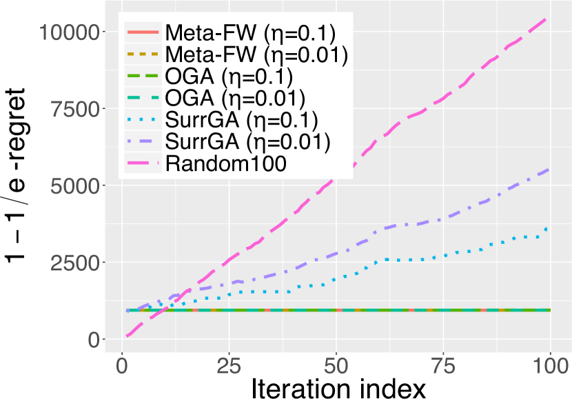
(a)

(b)

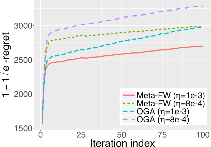
(c)

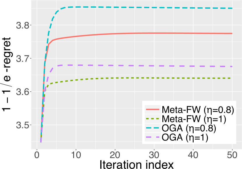
(d)

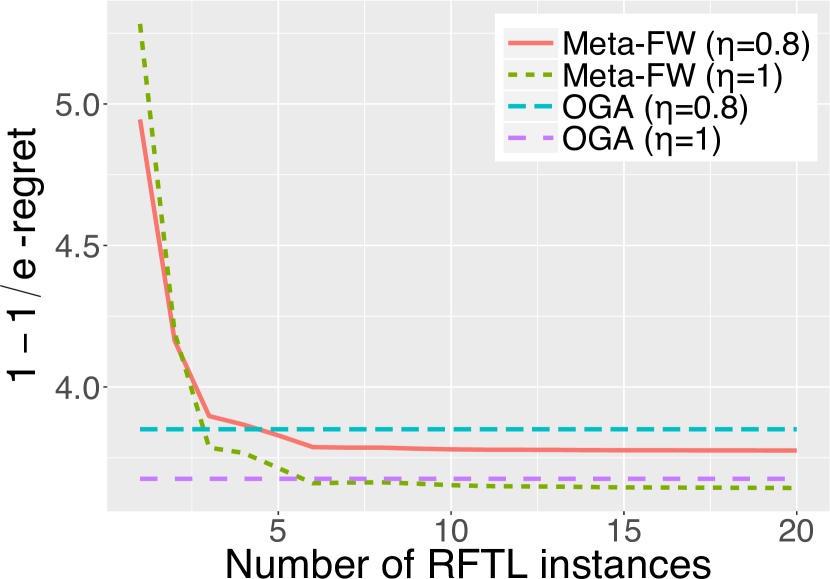
(e)

Figure 1: In the legends of all subfigures, we write Meta-FW for Meta-Frank-Wolfe, OGA for Online Gradient Ascent, and SurrGA for Surrogate Gradient Ascent. The results for the multilinear extension are presented in Figs. 1(a) and 1(b). We present the $(1-1/e)$-regret versus the number of iterations in Fig. 1(a). In Fig. 1(b) we illustrate the result for the setting in which only an unbiased estimate of the gradient is available. Fig. 1(c) shows how the $(1-1/e)$-regret evolves for the non-convex/non-concave quadratic programming. Figs. 1(d) and 1(e) are about the D-optimal experiment design problem. Fig. 1(d) shows the $(1-1/e)$-regret versus the number of iterations, while Fig. 1(e) shows how the number of RFTL instances $K$ influences the performance of Meta-Frank-Wolfe.

4.1 Multilinear Extension

As our first experiment, we consider a sequence of multilinear extensions of weighted coverage functions (see Section 2.2). Recall that such functions have a concave lower bound. Thus, we introduce another baseline Surrogate Gradient Ascent that uses supergradient ascent to maximize the concave lower bound function $(1-1/e)\bar{f}(\mathbf{x})$. The result is presented in Fig. 1(a). We observe that Random100 has the highest regret and both Meta-Frank-Wolfe and Online Gradient Ascent, whose performance is slightly inferior to that of Meta-Frank-Wolfe, outperform Surrogate Gradient Ascent.

Then, we study the case where only an unbiased estimate of the gradient is available. For any $\mathbf{x}\in[0,1]^{n}$, let

$$[\tilde{\nabla}f(\mathbf{x})]_{i}\triangleq f(R_{i}\cup\{i\})-f(R_{i}),$$

where $R_{i}$ is a random subset of $[n]\setminus\{i\}$ such that each $j\neq i$ is in $R_{i}$ with probability $x_{j}$ independently. Then we have $\mathbb{E}[\tilde{\nabla}f(\mathbf{x})]=\nabla f(\mathbf{x})$ (Calinescu et al., 2011). The result in this setting is presented in Fig. 1(b). Notice that in Fig. 1(b) the regret of Random100 and Surrogate Gradient Ascent is uninfluenced by the stochastic gradient oracle since they do not rely on the exact gradient of the original objective function. Meta-Frank-Wolfe and Online Gradient Ascent both incur higher regret in Fig. 1(b) than in Fig. 1(a). In addition, the stochastic gradient oracle has more impact upon Meta-Frank-Wolfe than Online Gradient Ascent. This agrees with our theoretical guarantee for Online Gradient Ascent and a result from (Hassani et al., 2017), which states that Frank-Wolfe-type algorithms are not robust to stochastic noise in the gradient oracle.

4.2 Non-Convex/Non-Concave Quadratic Programming

Quadratic programming problems have objective functions of the form $f(\mathbf{x})=\frac{1}{2}{\mathbf{x}}^{\top}\mathbf{H}{\mathbf{x}}+\mathbf{h}^{\top}{\mathbf{x}}+c$ and linear equality and/or inequality constraints. If the matrix $\mathbf{H}$ is indefinite, the objective function becomes non-convex and non-concave. We constructed $m$ linear inequality constraints $\mathbf{A}{\mathbf{x}}\leq\mathbf{b}$, where each entry of $\mathbf{A}\in\mathbb{R}^{m\times n}$ is sampled uniformly at random from $[0,1]$. We set $m=2$. In addition, we require that the variable ${\mathbf{x}}$ reside in a positive cuboid. Formally, the constraint is a positive polytope $\mathcal{P}=\{{\mathbf{x}}\in\mathbb{R}^{n}:\mathbf{A}{\mathbf{x}}\leq\mathbf{b},0\leq{\mathbf{x}}\leq\mathbf{u}\}$. We set $\mathbf{b}=\mathbf{u}=\mathbf{1}$. To ensure that the gradient is non-negative, we set $\mathbf{h}=-\mathbf{H}^{\top}\mathbf{u}$. Without loss of generality, we assume that the constant term $c$ is $0$. Thus the function is $f(\mathbf{x};\mathbf{H})=(\frac{1}{2}\mathbf{x}-\mathbf{u})^{\top}\mathbf{H}\mathbf{x}$; it is fully determined by the matrix $\mathbf{H}$. In our online optimization setting, we assume that the $T$ functions $f_{1},f_{2},\ldots,f_{T}$ are associated with matrices $\mathbf{H}_{1},\mathbf{H}_{2},\ldots,\mathbf{H}_{T}$. For every $\mathbf{H}_{i}$, its entries are sampled uniformly at random from $[-100,0]$. We set $K=50$. The result is illustrated in Fig. 1(c). It can be observed that with the same step size $\eta$, the regret of Meta-Frank-Wolfe is smaller than Online Gradient Ascent.

4.3 D-Optimal Experimental Design

The objective function of the D-optimal design problem is $f(\bm{\lambda})=\log\det\left(\sum_{i=1}^{N}\lambda_{i}{\bf x}_{i}{\bf x}_{i}^{\top}\right).$ We write $A(\bm{\lambda})$ for $\sum_{i=1}^{N}\lambda_{i}{\bf x}_{i}{\bf x}_{i}^{\top}$ for the ease of notation. It is DR-submodular because for any $i$ and $j$

$$\frac{\partial^{2}f(\bm{\lambda})}{\partial\lambda_{j}\partial\lambda_{i}}=-({\bf x}_{j}^{\top}A(\bm{\lambda})^{-1}{\bf x}_{i})^{2}\leq 0.$$

For every $\mathbf{x}_{i}$, its entries are sampled from the standard normal distribution independently. We try to solve the maximization in the polytope $\mathcal{P}=\{\bm{\lambda}:\mathbf{A}(\bm{\lambda}-\bm{1})\leq\bm{1},\bm{1}\leq\bm{\lambda}\leq\bm{2}\}$. Each entry of $\mathbf{A}$ is sampled uniformly from $[0,1]$ and the number of inequality constraints is set to $2$. The polytope is shifted to avoid $\bm{0}$ since the function is undefined at $\bm{\lambda}=\bm{0}$. In Fig. 1(d), we illustrate how the function value attained by the algorithms varies as it experiences more iterations; $K$ is fixed to be $50$ in this set of experiments. We observe that Meta-Frank-Wolfe outperforms all other baselines. In addition, Meta-Frank-Wolfe achieves better performance when the step size $\eta=1$.

In the second set of experiments, we show the function values attained by the algorithms at the end of the $50$th iteration, with $K$ ranging from $1$ to $20$ for Meta-Frank-Wolfe. Recall that $K$ is the number of Frank-Wolfe steps in Meta-Frank-Wolfe. The result is presented in Fig. 1(e). Since $K$ is not a parameter of Online Gradient Ascent, the regret of Online Gradient Ascent remains constant as $K$ varies. The regret of Meta-Frank-Wolfe is reduced as $K$ increases. This agrees with our intuition that more Frank-Wolfe steps yield better performance.

5 Related Work

Submodular functions.

Submodularity is a structural property that is often associated with set functions (Nemhauser et al., 1978; Fujishige, 2005). It has found far-reaching applications in statistics and artificial intelligence, including active learning (Golovin and Krause, 2011), viral marketing (Kempe et al., 2003; Gomez Rodriguez et al., 2012; Zhang et al., 2016), network monitoring (Leskovec et al., 2007; Gomez Rodriguez et al., 2010), document and corpus summarization (Lin and Bilmes, 2011; Kirchhoff and Bilmes, 2014; Sipos et al., 2012), crowd teaching (Singla et al., 2014), feature selection (Elenberg et al., 2016), and interpreting deep neural networks (Elenberg et al., 2017). However, submodularity goes beyond set functions and can be extended to continuous domains (Wolsey, 1982; Topkis, 1978). Maximizing a submodular set function is inherently related to its continuous relaxation through the multilinear extension (Calinescu et al., 2011), which is an example of the DR-submodular function. A variant of the Frank-Wolfe algorithm, called continuous greedy (Calinescu et al., 2011; Vondrák, 2008), can be used to maximize, within a $(1-1/e)$ approximation to the optimum, the multilinear extension of a submodular set function (Calinescu et al., 2011) or more generally a monotone smooth submodular function subject to a polytope (Chekuri et al., 2015). It is also known that finding a better approximation guarantee is impossible under reasonable complexity-theoretic assumptions (Feige, 1998; Vondrák, 2013). More recently, Bian et al. (2017) generalized the above results by considering the maximization of continuous DR-submodular functions subject to down-closed convex bodies and showed that the same continuous greedy method achieves a $(1-1/e)$ guarantee. In a different line of work, Hassani et al. (2017) studied the applicability of the (stochastic) gradient ascent algorithms to the stochastic continuous submodular maximization setting, where the objective function is defined in terms of an expectation. They proved that gradient methods achieve a $1/2$ approximation guarantee for monotone DR-submodular functions, subject to a general convex body. It is also known that gradient methods cannot achieve a better guarantee in general (Hassani et al., 2017; Vondrák et al., 2011). Furthermore, it is also shown in (Hassani et al., 2017) that the continuous greedy algorithms are not robust in stochastic settings (where only unbiased estimates of gradients are available) and can provide arbitrarily poor solutions, in general (thus motivating the need for stochastic projected gradient methods). Even though it is not the focus of this paper, we should mention that continuous submodular minimization has also been studied recently (Bach, 2015; Staib and Jegelka, 2017).

Online optimization.

Most of the work in online optimization considers convex (when minimizing the loss) or concave (when maximizing the reward) functions. The protocol of online convex optimization (OCO) was first defined by Zinkevich (2003). In his influential paper, he proposed the online gradient descent method and showed an $O(\sqrt{T})$ regret bound. The result was later improved to $O(\log(T))$ regret by Hazan et al. (2007) for strongly convex functions. Kalai and Vempala (2005) developed another class of algorithms termed Follow-The-Leader (FTL) with the idea of finding a point that minimizes the accumulated sum of all objective functions revealed so far. However, there are simple situations in which the regret of FTL grows linearly with $T$. To circumvent this issue, Kalai and Vempala (2005) introduced random perturbation as a regularization and proposed the follow-the-perturbed-leader algorithm, following an early work (Hannan, 1957). In addition, Shalev-Shwartz and Singer (2007) and Abernethy et al. (2008a) designed the regularized-follow-the-leader (RFTL) algorithm. A comprehensive survey of OCO can be found in (Hazan, 2016; Shalev-Shwartz et al., 2012). Recently, Lafond et al. (2015) studied the setting in which the loss functions $\{f_{t}:1\leq t\leq T\}$ are drawn i.i.d. from a fixed distribution and proposed the online Frank-Wolfe algorithm. They showed an $O(\log^{3}(T))$ regret for strongly convex loss functions. Furthermore, they showed that their algorithm finds a stationary point to the stochastic loss at a rate of $O(\sqrt{1/T})$. Garber and Hazan (2013) proposed a conditional gradient algorithm for online convex optimization problem over polyhedral sets. Only a single linear optimization step is performed in each iteration and this algorithm achieves $O(\sqrt{T})$ regret bound for convex losses and $O(\log T)$ regret bound for strongly convex losses. Luo and Schapire (2014) proposed a general methodology for devising online learning algorithms based on a drifting-games analysis. Hazan et al. (2017) goes beyond convexity and considered regret minimization in repeated games with non-convex loss functions. They introduced a new objective termed local regret and proposed online non-convex optimization algorithms that achieve optimal guarantees for this new objective. Our work, in contrast, considers non-convex objective functions that can be approximately maximized. In our notion of $\alpha$-regret, we design two algorithms that can compete with the best fixed offline approximate solution (and not necessarily the stationary points) with tight regret bounds.

Online submodular optimization.

Existing work considered online submodular optimization in a discrete domain. Streeter and Golovin (2009) and Golovin et al. (2014) proposed online optimization algorithms for submodular set functions under cardinality and matroid constraints, respectively. Our work studies the online submodular optimization in continuous domains. We should point out that the online algorithm proposed in Golovin et al. (2014) relies on the multilinear continuous relaxation, which is simply an instance of the general class of DR-submodular functions that we consider here.

6 Conclusion

In this paper, we considered an online optimization process, where the objective functions were continuous DR-submodular. We proposed two online optimization algorithms, Meta-Frank-Wolfe (that has access to exact gradients) and Online Gradient Ascent (that only has access to unbiased estimates of the gradients), both with no-regret guarantees. We also evaluated the performance of our algorithms in practice. Our results make an important contribution in providing performance guarantees for a subclass of online non-convex optimization problems.

Acknowledgments

This work was supported by AFOSR YIP award (FA9550-18-1-0160).

Appendix A Proof of Theorem 1

Before presenting the proof of Theorem 1, we need two lemmas first. Lemma 1 shows that a $\beta$-smooth function can be bounded by quadratic functions from above and below. Lemma 2 shows the concavity of continuous DR-submodular functions along non-negative and non-positive directions.

Lemma 1.

If $f$ is $\beta$-smooth, then we have for any $\mathbf{x}$ and $\mathbf{y}$,

$$\left|f(\mathbf{x})-f(\mathbf{y})-\nabla f(\mathbf{x})^{\top}(\mathbf{x}-\mathbf{y})\right|\leq\frac{\beta}{2}\lVert\mathbf{x}-\mathbf{y}\rVert^{2}.$$

$$\left|f(\mathbf{x})-f(\mathbf{y})-\nabla f(\mathbf{y})^{\top}(\mathbf{x}-\mathbf{y})\right|\leq\frac{\beta}{2}\lVert\mathbf{x}-\mathbf{y}\rVert^{2}.$$

Proof.

Let us define an auxiliary function $g(t)=f(\mathbf{x}+t(\mathbf{y}-\mathbf{x}))$. We observe that $g(0)=f(\mathbf{x})$ and $g(1)=f(\mathbf{y})$. The derivative of $g(t)$ is

$$g^{\prime}(t)=\nabla f(\mathbf{x}+t(\mathbf{y}-\mathbf{x}))^{\top}(\mathbf{y}-\mathbf{x}).$$

We have

$$f(\mathbf{y})-f(\mathbf{x})=g(1)-g(0)=\int_{0}^{1}g^{\prime}(t)dt=\int_{0}^{1}\nabla f(\mathbf{x}+t(\mathbf{y}-\mathbf{x}))^{\top}(\mathbf{y}-\mathbf{x})dt.$$

The left-hand side of the first inequality is equal to

$$\left|\int_{0}^{1}\nabla f(\mathbf{x}+t(\mathbf{y}-\mathbf{x}))^{\top}(\mathbf{x}-\mathbf{y})dt-\nabla f(\mathbf{x})^{\top}(\mathbf{x}-\mathbf{y})\right|=\left|\int_{0}^{1}(\nabla f(\mathbf{x}+t(\mathbf{y}-\mathbf{x}))-\nabla f(\mathbf{x}))^{\top}(\mathbf{x}-\mathbf{y})\right|dt\leq\int_{0}^{1}\left|(\nabla f(\mathbf{x}+t(\mathbf{y}-\mathbf{x}))-\nabla f(\mathbf{x}))^{\top}(\mathbf{x}-\mathbf{y})\right|dt\leq\int_{0}^{1}\lVert\nabla f(\mathbf{x}+t(\mathbf{y}-\mathbf{x}))-\nabla f(\mathbf{x})\rVert\lVert\mathbf{x}-\mathbf{y}\rVert dt\leq\int_{0}^{1}\beta t\lVert\mathbf{x}-\mathbf{y}\rVert^{2}dt=\frac{\beta}{2}\lVert\mathbf{x}-\mathbf{y}\rVert.$$

Exchanging $\mathbf{x}$ and $\mathbf{y}$ in the first inequality, we obtain the second one immediately. ∎

Lemma 2 (Proposition 4 in Bian et al. (2017)).

A continuous DR-submodular function is concave along any non-negative direction and any non-positive direction.

Lemma 2 implies that if $f$ is continuous DR-submodular, fixing any $x$ in its domain, $g(z)\triangleq f(\mathbf{x}+z\mathbf{v})$ is concave in $z$ as long as $\mathbf{v}\geq 0$ holds elementwise. Now we present the proof of Theorem 1.

Proof.

As the first step, let us fix $t$ and $k$. Since $f_{t}$ is $\beta$-smooth, by Lemma 1, for any $\xi\geq 0$ and ${\bf x},{\bf v}\in\mathbb{R}_{\geq 0}^{n}$, we have

$$f_{t}(\mathbf{x}+\xi\mathbf{v})-f_{t}(\mathbf{x})-\nabla f_{t}(\mathbf{x})^{\top}(\xi\mathbf{v})\geq-\frac{\beta}{2}\lVert\xi\mathbf{v}\rVert^{2}$$

Let $L\triangleq\beta R^{2}$. We deduce

$$f_{t}({\bf x}_{t}(k+1))-f_{t}({\bf x}_{t}(k))=f_{t}({\bf x}_{t}(k)+\frac{1}{K}{\bf v}_{t}^{k})-f_{t}({\bf x}_{t}(k))\geq\frac{1}{K}\langle{\bf v}_{t}^{k},\nabla f_{t}({\bf x}_{t}(k))\rangle-\frac{L}{2K^{2}}.$$

We sum the above equation over $t$ and obtain

$$\sum_{t=1}^{T}f_{t}({\bf x}_{t}(k+1))-f_{t}({\bf x}_{t}(k))\geq\sum_{t=1}^{T}\frac{1}{K}\langle{\bf v}_{t}^{k},\nabla f_{t}({\bf x}_{t}(k))\rangle-\frac{LT}{2K^{2}}.$$

The RFTL algorithm instance $\mathcal{E}^{k}$ finds $\{{\bf v}_{t}^{k}:1\leq t\leq T\}$ such that

$$\sum_{t=1}^{T}\langle{\bf v}^{k*},\nabla f_{t}({\bf x}_{t}(k))\rangle-\sum_{t=1}^{T}\langle{\bf v}_{t}^{k},\nabla f_{t}({\bf x}_{t}(k))\rangle\leq r^{k}\leq 2DG\sqrt{T},$$

where

$${\bf v}^{k*}=\operatorname*{arg\,max}_{{\bf v}\in\mathcal{P}}\sum_{t=1}^{T}\langle{\bf v},\nabla f_{t}({\bf x}_{t}(k))\rangle$$

and $r^{k}$ is the total regret that the RFTL instance suffers by the end of the $T$th iteration. According to the regret bound of the RFTL, we know that $r^{k}\leq 2DG\sqrt{T}$. Therefore,

$$\sum_{t=1}^{T}f_{t}({\bf x}_{t}(k+1))-f_{t}({\bf x}_{t}(k))\geq\frac{1}{K}\left(\sum_{t=1}^{T}\langle{\bf v}^{k*},\nabla f_{t}({\bf x}_{t}(k))\rangle-r^{k}\right)-\frac{LT}{2K^{2}}.$$

We define ${\bf x}^{*}\triangleq\operatorname*{arg\,max}_{{\bf v}\in\mathcal{P}}\sum_{t=1}^{T}f_{t}({\bf v})$ and ${\bf w}_{t}^{k}=({\bf x}^{*}-{\bf x}_{t}(k))\vee 0$. For every $t$, we have ${\bf w}_{t}^{k}=({\bf x}^{*}-{\bf x}_{t}(k))\vee 0\leq{\bf x}^{*}$. It is obvious that ${\bf w}_{t}^{k}\geq 0$. Therefore we deduce that ${\bf w}_{t}^{k}\in\mathcal{X}$. Due to the concavity of $f_{t}$ along any non-negative direction (see Lemma 2), we have

$$f_{t}({\bf x}_{t}(k)+{\bf w}_{t}^{k})-f_{t}({\bf x}_{t}(k))\leq\langle{\bf w}_{t}^{k},\nabla f_{t}({\bf x}_{t}(k))\rangle.$$

In light of the above equation, we obtain a lower bound for $\sum_{t=1}^{T}\langle{\bf v}^{k*},\nabla f_{t}({\bf x}_{t}(k))\rangle$:

$$\sum_{t=1}^{T}\langle{\bf v}^{k*},\nabla f_{t}({\bf x}_{t}(k))\rangle\geq \sum_{t=1}^{T}\langle\mathbf{x}^{*},\nabla f_{t}({\bf x}_{t}(k))\rangle$$

$$\stackrel{{\scriptstyle(a)}}{{\geq}} \sum_{t=1}^{T}\langle{\bf w}_{t}^{k},\nabla f_{t}({\bf x}_{t}(k))\rangle$$

$$\geq \sum_{t=1}^{T}(f_{t}({\bf x}_{t}(k)+{\bf w}_{t}^{k})-f_{t}({\bf x}_{t}(k)))$$

$$= \sum_{t=1}^{T}(f_{t}({\bf x}^{*}\vee{\bf x}_{t}(k))-f_{t}({\bf x}_{t}(k)))$$

$$\geq \sum_{t=1}^{T}(f_{t}({\bf x}^{*})-f_{t}({\bf x}_{t}(k))).$$

We use the fact that $\nabla f_{t}({\bf x}_{t}(k))\geq 0$ and $\mathbf{x}^{*}\geq\mathbf{w}_{t}^{k}$ entrywise in the inequality (a).

$$\sum_{t=1}^{T}f_{t}({\bf x}_{t}(k+1))-f_{t}({\bf x}_{t}(k))\geq\frac{1}{K}\left(\sum_{t=1}^{T}(f_{t}({\bf x}^{*})-f_{t}({\bf x}_{t}(k)))-r^{k}\right)-\frac{LT}{2K^{2}}.$$

After rearrangement,

$$\sum_{t=1}^{T}\left(f_{t}({\bf x}_{t}(k+1))-f_{t}({\bf x}^{*})\right)\geq(1-\frac{1}{K})\sum_{t=1}^{T}\left(f_{t}({\bf x}_{t}(k))-f_{t}({\bf x}^{*})\right)-\frac{1}{K}r^{k}-\frac{LT}{2K^{2}}.$$

Therefore,

$$\sum_{t=1}^{T}\left(f_{t}({\bf x}_{t}(K))-f_{t}({\bf x}^{*})\right)\geq(1-\frac{1}{K})^{K}\sum_{t=1}^{T}\left(f_{t}({\bf x}_{t}(0))-f_{t}({\bf x}^{*})\right)-\frac{1}{K}\sum_{k=0}^{K-1}r^{k}-\frac{LT}{2K}=(1-\frac{1}{K})^{K}\sum_{t=1}^{T}\left(f_{t}(0)-f_{t}({\bf x}^{*})\right)-\frac{1}{K}\sum_{k=0}^{K-1}r^{k}-\frac{LT}{2K}.$$

Since $(1-\frac{1}{K})^{K}\leq e^{-1}$, we have

$$\sum_{t=1}^{T}\left(f_{t}({\bf x}^{*})-f_{t}({\bf x}_{t}(K))\right)\leq(1-\frac{1}{K})^{K}\sum_{t=1}^{T}\left(f_{t}({\bf x}^{*})-f_{t}(0)\right)+\frac{1}{K}\sum_{k=0}^{K-1}r^{k}+\frac{LT}{2K}\leq e^{-1}\sum_{t=1}^{T}\left(f_{t}({\bf x}^{*})-f_{t}(0)\right)+\frac{1}{K}\sum_{k=0}^{K-1}r^{k}+\frac{LT}{2K}.$$

After rearrangement, we have

$$\sum_{t=1}^{T}f_{t}({\bf x}_{t}(K))\geq(1-1/e)\sum_{t=1}^{T}f_{t}({\bf x}^{*})+e^{-1}\sum_{t=1}^{T}f_{t}(0)-\frac{1}{K}\sum_{k=0}^{K-1}r^{k}-\frac{LT}{2K^{2}}.$$

Plugging in the definition of $r^{k}$ gives

$$\sum_{t=1}^{T}f_{t}({\bf x}_{t})=\sum_{t=1}^{T}f_{t}({\bf x}_{t}(K))\geq(1-1/e)\sum_{t=1}^{T}f_{t}({\bf x}^{*})+e^{-1}\sum_{t=1}^{T}f_{t}(0)-2DG\sqrt{T}-\frac{LT}{2K}.$$

Recall that $\mathbf{x}_{t}(K)$ is exactly $\mathbf{x}_{t}$. Thus equivalently, we have

$$(1-1/e)\sum_{t=1}^{T}f_{t}({\bf x}^{*})-\sum_{t=1}^{T}f_{t}({\bf x}_{t})\leq-e^{-1}\sum_{t=1}^{T}f_{t}(0)+2DG\sqrt{T}+\frac{\beta R^{2}T}{2K}.$$

∎

Appendix B Proof of Theorem 2

B.1 Gradient Ascent Case

The theoretical guarantee of gradient ascent methods applied to concave functions relies on a pivotal property that characterizes concavity: if $F$ is concave, then $F(\mathbf{y})-F(\mathbf{x})\leq\langle\nabla F(\mathbf{x}),\mathbf{y}-\mathbf{x}\rangle$. Fortunately, there is a similar property that holds for monotone weakly DR-submodular functions, which is presented in Lemma 3.

Lemma 3.

Let $F:\mathcal{X}\to\mathbb{R}_{+}$ be a monotone and weakly DR-submodular function with parameter $\gamma$. For any two vector ${\bf x},{\bf y}\in\mathcal{X}$, we have

$$F({\bf y})-\left(1+\frac{1}{\gamma^{2}}\right)F({\bf x})\leq\frac{1}{\gamma}\left\langle\nabla F({\bf x}),{\bf y}-{\bf x}\right\rangle.$$

The proof of Lemma 3 can be found in the proof of Theorem 4.2 in (Hassani et al., 2017). Now we can prove Theorem 2 in the gradient ascent case.

Proof.

Let ${\bf x}^{*}=\operatorname*{arg\,max}_{{\bf x}\in\mathcal{P}}\sum_{t=1}^{T}f_{t}({\bf x})$. We define $\nabla_{t}\triangleq\nabla f_{t}({\bf x}_{t})$. By the definition of $\mathbf{x}_{t+1}$ and properties of the projection operator for a convex set, we have

$$\left\|{\bf x}_{t+1}-{\bf x}^{*}\right\|^{2}=\left\|\Pi_{\mathcal{P}}({\bf x}_{t}+\eta_{t}\nabla_{t})-{\bf x}^{*}\right\|^{2}\leq\left\|{\bf x}_{t}+\eta_{t}\nabla_{t}-{\bf x}^{*}\right\|^{2}\leq\left\|{\bf x}_{t}-{\bf x}^{*}\right\|^{2}+\eta_{t}^{2}\left\|\nabla_{t}\right\|^{2}-2\eta_{t}\nabla_{t}^{\top}({\bf x}^{*}-{\bf x}_{t}).$$

Therefore we deduce

$$\nabla_{t}^{\top}({\bf x}^{*}-{\bf x}_{t}) \leq\frac{\left\|{\bf x}_{t}-{\bf x}^{*}\right\|^{2}-\left\|{\bf x}_{t+1}-{\bf x}^{*}\right\|^{2}+\eta_{t}^{2}\left\|\nabla_{t}\right\|^{2}}{2\eta_{t}}$$

$$\leq\frac{\left\|{\bf x}_{t}-{\bf x}^{*}\right\|^{2}-\left\|{\bf x}_{t+1}-{\bf x}^{*}\right\|^{2}}{2\eta_{t}}+\frac{\eta_{t}G^{2}}{2}$$

By Lemma 3, we obtain that

$$f_{t}({\bf x}^{*})-\left(1+\frac{1}{\gamma^{2}}\right)f({\bf x}_{t})\leq\frac{1}{\gamma}\left\langle\nabla_{t},{\bf x}^{*}-{\bf x}_{t}\right\rangle.$$

If we define $\frac{1}{\eta_{0}}\triangleq 0$, it can be deduced that

$$\sum_{t=1}^{T}\left[f_{t}({\bf x}^{*})-\left(1+\frac{1}{\gamma^{2}}\right)f_{t}({\bf x}_{t})\right]\leq\frac{1}{\gamma}\sum_{t=1}^{T}\nabla_{t}^{\top}({\bf x}^{*}-{\bf x}_{t})\leq\frac{1}{\gamma}\left[\frac{1}{2\eta_{t}}\sum_{t=1}^{T}\left(\left\|{\bf x}_{t}-{\bf x}^{*}\right\|^{2}-\left\|{\bf x}_{t+1}-{\bf x}^{*}\right\|^{2}\right)+\frac{G^{2}}{2}\sum_{t=1}^{T}\eta_{t}\right]\leq\frac{1}{\gamma}\left[\frac{1}{2}\left(\sum_{t=1}^{T}\left\|{\bf x}_{t}-{\bf x}^{*}\right\|^{2}(\frac{1}{\eta_{t}}-\frac{1}{\eta_{t-1}})\right)+\frac{G^{2}}{2}\sum_{t=1}^{T}\eta_{t}\right]\leq\frac{1}{\gamma}\left[\frac{D^{2}}{2\eta_{T}}+\frac{G^{2}}{2}\sum_{t=1}^{T}\eta_{t}\right]\leq\frac{3}{2\gamma}DG\sqrt{T}.$$

After rearrangement, it is clear that

$$\frac{\gamma^{2}}{\gamma^{2}+1}\sum_{t=1}^{T}f_{t}({\bf x}^{*})-\sum_{t=1}^{T}f_{t}({\bf x}_{t})\leq\frac{3\gamma DG\sqrt{T}}{2(\gamma^{2}+1)}.$$

∎

B.2 Stochastic Gradient Ascent Case

Proof.

The strategy for the stochastic gradient ascent case is similar to that of the gradient ascent case. Again, by the definition of $\mathbf{x}_{t+1}$, we have

$$\left\|{\bf x}_{t+1}-{\bf x}^{*}\right\|^{2}=\left\|\Pi_{\mathcal{P}}({\bf x}_{t}+\eta_{t}\mathbf{g}_{t})-{\bf x}^{*}\right\|^{2}\leq\left\|{\bf x}_{t}+\eta_{t}\mathbf{g}_{t}-{\bf x}^{*}\right\|^{2}\leq\left\|{\bf x}_{t}-{\bf x}^{*}\right\|^{2}+\eta_{t}^{2}\left\|{\bf g}_{t}\right\|^{2}-2\eta_{t}{\bf g}_{t}^{\top}({\bf x}^{*}-{\bf x}_{t})$$

Therefore we deduce

$${\bf g}_{t}^{\top}({\bf x}^{*}-{\bf x}_{t})\leq\frac{\left\|{\bf x}_{t}-{\bf x}^{*}\right\|^{2}-\left\|{\bf x}_{t+1}-{\bf x}^{*}\right\|^{2}+\eta_{t}^{2}\left\|{\bf g}_{t}\right\|^{2}}{2\eta_{t}}\leq\frac{\left\|{\bf x}_{t}-{\bf x}^{*}\right\|^{2}-\left\|{\bf x}_{t+1}-{\bf x}^{*}\right\|^{2}}{2\eta_{t}}+\frac{\eta_{t}G^{2}}{2}$$

Similarly, if we define $\frac{1}{\eta_{0}}\triangleq 0$ and in light of Lemma 3, it can be deduced that

$$\sum_{t=1}^{T}\mathbb{E}\left[f_{t}({\bf x}^{*})-\left(1+\frac{1}{\gamma^{2}}\right)f_{t}({\bf x}_{t})\right]\leq\frac{1}{\gamma}\sum_{t=1}^{T}\mathbb{E}\left[\nabla_{t}^{\top}({\bf x}^{*}-{\bf x}_{t})\right]=\frac{1}{\gamma}\sum_{t=1}^{T}\mathbb{E}\left[\mathbb{E}\left[\nabla_{t}^{\top}({\bf x}^{*}-{\bf x}_{t})|{\bf x}_{t}\right]\right]=\frac{1}{\gamma}\sum_{t=1}^{T}\mathbb{E}\left[\mathbb{E}\left[{\bf g}_{t}^{\top}({\bf x}^{*}-{\bf x}_{t})|{\bf x}_{t}\right]\right]\leq\frac{1}{\gamma}\left[\frac{1}{2\eta_{t}}\sum_{t=1}^{T}\mathbb{E}\left[\left\|{\bf x}_{t}-{\bf x}^{*}\right\|^{2}-\left\|{\bf x}_{t+1}-{\bf x}^{*}\right\|^{2}\right]+\frac{G^{2}}{2}\sum_{t=1}^{T}\eta_{t}\right]\leq\frac{1}{\gamma}\left[\frac{1}{2}\left(\sum_{t=1}^{T}\mathbb{E}\left[\left\|{\bf x}_{t}-{\bf x}^{*}\right\|^{2}\right](\frac{1}{\eta_{t}}-\frac{1}{\eta_{t-1}})\right)+\frac{G^{2}}{2}\sum_{t=1}^{T}\eta_{t}\right]\leq\frac{1}{\gamma}\left[\frac{D^{2}}{2\eta_{T}}+\frac{G^{2}}{2}\sum_{t=1}^{T}\eta_{t}\right]\leq\frac{3}{2\gamma}DG\sqrt{T}.$$

After rearrangement, it is clear that

$$\frac{\gamma^{2}}{\gamma^{2}+1}\sum_{t=1}^{T}f_{t}({\bf x}^{*})-\sum_{t=1}^{T}\mathbb{E}\left[f_{t}({\bf x}_{t})\right]\leq\frac{3\gamma DG\sqrt{T}}{2(\gamma^{2}+1)}.$$

∎

References

- Abernethy et al. (2008a) Jacob D Abernethy, Elad Hazan, and Alexander Rakhlin. Competing in the dark: An efficient algorithm for bandit linear optimization. In COLT, pages 263–274, 2008a.
- Abernethy et al. (2008b) Jacob Duncan Abernethy, Elad Hazan, and Alexander Rakhlin. An efficient algorithm for bandit linear optimization. In COLT, 2008b.
- Bach (2015) Francis Bach. Submodular functions: from discrete to continous domains. arXiv preprint arXiv:1511.00394, 2015.
- Bian et al. (2017) An Bian, Baharan Mirzasoleiman, Joachim M. Buhmann, and Andreas Krause. Guaranteed non-convex optimization: Submodular maximization over continuous domains. In AISTATS, February 2017.
- Calinescu et al. (2011) Gruia Calinescu, Chandra Chekuri, Martin Pál, and Jan Vondrák. Maximizing a monotone submodular function subject to a matroid constraint. SIAM Journal on Computing, 40(6):1740–1766, 2011.
- Chekuri et al. (2015) Chandra Chekuri, TS Jayram, and Jan Vondrák. On multiplicative weight updates for concave and submodular function maximization. In Proceedings of the 2015 Conference on Innovations in Theoretical Computer Science, pages 201–210. ACM, 2015.
- Eghbali and Fazel (2016) Reza Eghbali and Maryam Fazel. Designing smoothing functions for improved worst-case competitive ratio in online optimization. In NIPS, pages 3287–3295, 2016.
- Elenberg et al. (2016) Ethan R Elenberg, Rajiv Khanna, Alexandros G Dimakis, and Sahand Negahban. Restricted strong convexity implies weak submodularity. arXiv preprint arXiv:1612.00804, 2016.
- Elenberg et al. (2017) Ethan R Elenberg, Alexandros G Dimakis, Moran Feldman, and Amin Karbasi. Streaming weak submodularity: Interpreting neural networks on the fly. In NIPS, page to appear, 2017.
- Feige (1998) Uriel Feige. A threshold of ln n for approximating set cover. Journal of the ACM (JACM), 45(4):634–652, 1998.
- Fujishige (2005) Satoru Fujishige. Submodular functions and optimization, volume 58. Elsevier, 2005.
- Garber and Hazan (2013) Dan Garber and Elad Hazan. A linearly convergent conditional gradient algorithm with applications to online and stochastic optimization. arXiv preprint arXiv:1301.4666, 2013.
- Golovin and Krause (2011) Daniel Golovin and Andreas Krause. Adaptive submodularity: Theory and applications in active learning and stochastic optimization. JAIR, 42:427–486, 2011.
- Golovin et al. (2014) Daniel Golovin, Andreas Krause, and Matthew Streeter. Online submodular maximization under a matroid constraint with application to learning assignments. Technical report, arXiv, 2014.
- Gomez Rodriguez et al. (2012) M Gomez Rodriguez, B Schölkopf, Langford J Pineau, et al. Influence maximization in continuous time diffusion networks. In ICML, pages 1–8. International Machine Learning Society, 2012.
- Gomez Rodriguez et al. (2010) Manuel Gomez Rodriguez, Jure Leskovec, and Andreas Krause. Inferring networks of diffusion and influence. In SIGKDD, pages 1019–1028. ACM, 2010.
- Gottschalk and Peis (2015) Corinna Gottschalk and Britta Peis. Submodular function maximization on the bounded integer lattice. In International Workshop on Approximation and Online Algorithms, pages 133–144. Springer, 2015.
- Hannan (1957) James Hannan. Approximation to bayes risk in repeated play. Contributions to the Theory of Games, 3:97–139, 1957.
- Hassani et al. (2017) Hamed Hassani, Mahdi Soltanolkotabi, and Amin Karbasi. Gradient methods for submodular maximization. arXiv preprint arXiv:1708.03949, 2017.
- Hazan (2016) Elad Hazan. Introduction to online convex optimization. Foundations and Trends® in Optimization, 2(3-4):157–325, 2016.
- Hazan et al. (2007) Elad Hazan, Amit Agarwal, and Satyen Kale. Logarithmic regret algorithms for online convex optimization. Machine Learning, 69(2):169–192, 2007.
- Hazan et al. (2017) Elad Hazan, Karan Singh, and Cyril Zhang. Efficient regret minimization in non-convex games. arXiv preprint arXiv:1708.00075, 2017.
- Kakade et al. (2009) Sham M Kakade, Adam Tauman Kalai, and Katrina Ligett. Playing games with approximation algorithms. SIAM Journal on Computing, 39(3):1088–1106, 2009.
- Kalai and Vempala (2005) Adam Kalai and Santosh Vempala. Efficient algorithms for online decision problems. Journal of Computer and System Sciences, 71(3):291–307, 2005.
- Karimi et al. (2017) Mohammad Karimi, Mario Lucic, Hamed Hassani, and Andreas Krause. Stochastic submodular maximization: The case of coverage functions. In NIPS, page to appear, 2017.
- Kempe et al. (2003) David Kempe, Jon Kleinberg, and Éva Tardos. Maximizing the spread of influence through a social network. In SIGKDD, pages 137–146. ACM, 2003.
- Kirchhoff and Bilmes (2014) Katrin Kirchhoff and Jeff Bilmes. Submodularity for data selection in statistical machine translation. In EMNLP, pages 131–141, 2014.
- Lafond et al. (2015) Jean Lafond, Hoi-To Wai, and Eric Moulines. On the online Frank-Wolfe algorithms for convex and non-convex optimizations. arXiv preprint arXiv:1510.01171, 2015.
- Leskovec et al. (2007) Jure Leskovec, Andreas Krause, Carlos Guestrin, Christos Faloutsos, Jeanne VanBriesen, and Natalie Glance. Cost-effective outbreak detection in networks. In SIGKDD, pages 420–429. ACM, 2007.
- Lin and Bilmes (2011) Hui Lin and Jeff Bilmes. A class of submodular functions for document summarization. In ACL, pages 510–520, 2011.
- Luo and Schapire (2014) Haipeng Luo and Robert E Schapire. A drifting-games analysis for online learning and applications to boosting. In NIPS, pages 1368–1376, 2014.
- Nemhauser et al. (1978) George L Nemhauser, Laurence A Wolsey, and Marshall L Fisher. An analysis of approximations for maximizing submodular set functions—i. Mathematical Programming, 14(1):265–294, 1978.
- Sankappanavar and Burris (1981) Hanamantagouda P Sankappanavar and Stanley Burris. A course in universal algebra, volume 78 of Graduate Texts in Mathematics. 1981.
- Shalev-Shwartz (2007) Shai Shalev-Shwartz. Online learning: Theory, algorithms, and applications. PhD thesis, The Hebrew University of Jerusalem, 2007.
- Shalev-Shwartz and Singer (2007) Shai Shalev-Shwartz and Yoram Singer. A primal-dual perspective of online learning algorithms. Machine Learning, 69(2-3):115–142, 2007.
- Shalev-Shwartz et al. (2012) Shai Shalev-Shwartz et al. Online learning and online convex optimization. Foundations and Trends® in Machine Learning, 4(2):107–194, 2012.
- Singla et al. (2014) Adish Singla, Ilija Bogunovic, Gábor Bartók, Amin Karbasi, and Andreas Krause. Near-optimally teaching the crowd to classify. In ICML, pages 154–162, 2014.
- Sipos et al. (2012) Ruben Sipos, Adith Swaminathan, Pannaga Shivaswamy, and Thorsten Joachims. Temporal corpus summarization using submodular word coverage. In CIKM, pages 754–763. ACM, 2012.
- Soma and Yoshida (2016) Tasuku Soma and Yuichi Yoshida. Maximizing monotone submodular functions over the integer lattice. In International Conference on Integer Programming and Combinatorial Optimization, pages 325–336. Springer, 2016.
- Staib and Jegelka (2017) Matthew Staib and Stefanie Jegelka. Robust budget allocation via continuous submodular functions. In ICML, pages 3230–3240, 2017.
- Streeter and Golovin (2009) Matthew Streeter and Daniel Golovin. An online algorithm for maximizing submodular functions. In NIPS, pages 1577–1584, 2009.
- Topkis (1978) Donald M Topkis. Minimizing a submodular function on a lattice. Operations research, 26(2):305–321, 1978.
- Vondrák (2007) Jan Vondrák. Submodularity in combinatorial optimization. PhD thesis, Charles University, 2007.
- Vondrák (2008) Jan Vondrák. Optimal approximation for the submodular welfare problem in the value oracle model. In STOC, pages 67–74. ACM, 2008.
- Vondrák (2013) Jan Vondrák. Symmetry and approximability of submodular maximization problems. SIAM Journal on Computing, 42(1):265–304, 2013.
- Vondrák et al. (2011) Jan Vondrák, Chandra Chekuri, and Rico Zenklusen. Submodular function maximization via the multilinear relaxation and contention resolution schemes. In STOC, pages 783–792. ACM, 2011.
- Wolsey (1982) Laurence A Wolsey. An analysis of the greedy algorithm for the submodular set covering problem. Combinatorica, 2(4):385–393, 1982.
- Zhang et al. (2016) Yuanxing Zhang, Yichong Bai, Lin Chen, Kaigui Bian, and Xiaoming Li. Influence maximization in messenger-based social networks. In Proceedings of IEEE GLOBECOM 2016, Washington D.C., USA, December 4–8 2016.
- Zinkevich (2003) Martin Zinkevich. Online convex programming and generalized infinitesimal gradient ascent. In ICML, pages 928–936, 2003.