Dark-bright soliton pairs: bifurcations and collisions

Abstract

The statics, stability and dynamical properties of dark-bright soliton pairs are investigated motivated by applications in a homogeneous system of two-component repulsively interacting Bose-Einstein condensate. One of the intra-species interaction coefficients is used as the relevant parameter controlling the deviation from the integrable Manakov limit. Two different families of stationary states are identified consisting of dark-bright solitons that are either antisymmetric (out-of-phase) or asymmetric (mass imbalanced) with respect to their bright soliton. Both of the above dark-bright configurations coexist at the integrable limit of equal intra- and inter-species repulsions and are degenerate in that limit. However, they are found to bifurcate from it in a transcritical bifurcation. The latter interchanges the stability properties of the bound dark-bright pairs rendering the antisymmetric states unstable and the asymmetric ones stable past the associated critical point (and vice versa before it). Finally, on the dynamical side, it is found that large kinetic energies and thus rapid soliton collisions are essentially unaffected by the intra-species variation, while cases involving near equilibrium states or breathing dynamics are significantly modified under such a variation.

I Introduction

Multi-component Bose-Einstein condensates (BECs) and the nonlinear excitations that arise in them have been a focal research point over the past two decades since their experimental realization gpes1 ; gpes2 . Among these excitations, dark-bright (DB) solitons constitute a fundamental example frantzkevre , whose experimental realization in a ⁸⁷Rb mixture hamburg has triggered a new era of investigations regarding the stability and interactions of these matter waves both with each other yan , as well as induced by the external traps ba ; hamner ; middelkamp ; alvarez .

Within mean-field theory the static and dynamical properties of such states are well described by a system of coupled Gross-Pitaevskii equations gpes1 ; gpes2 . The latter is a variant of the so-called defocusing (repulsive) vector nonlinear Schrödinger equation nls ; siambook , to which it reduces in the absence of a confining potential. In this homogeneous setting, single DB solitons exist as exact analytical solutions when the repulsive interactions within (intra-) and between (inter-) the species are of equal strength; this is the integrable, so-called Manakov limit manakov . In this setting, multiple solitonic states, both static and travelling ones, have been analytically derived by using the inverse scattering transform (IST) considering both trivial manakov , or more recently, non-trivial boundary conditions prinari ; biondini allowing also for energy (and phase) exchanges between the bright soliton components. Additionally, the Hirota method has been used to explore different families of DB soliton solutions ranging from perfectly antisymmetric (out-of-phase) to fully asymmetric ones (mass imbalanced), with respect to their bright soliton counterpart shepkiv (see also for a small sample among numerous additional studies the works vdbysk1 ; ralak ; parkshin ; rajendran ).

As a matter of fact, given their versatility, BECs offer additional layers of tunability, enabling the controllable departure from this integrable Manakov limit. In particular, exploiting the tunablility of both the inter- and intra-species scattering lengths that can be achieved in current experimental settings with the aid of Feshbach resonances inouye ; roberts ; donley ; thalhammer ; chin , a new avenue opened towards exploring DB soliton interactions under parametric variations ef ; et ; ljpp ; carr ; ljpp1 . This allowed to address the robustness of these matter waves in BEC mixtures with genuinely different scattering lengths. However, typically in realistic settings all three coefficients of inter- and intra- component interactions are slightly different, and hence it is of particular interest to explore how things deviate from the integrable limit.

In the present work, our aim is to bring to bear the enhanced understanding of the integrable limit that exists through the recent works of prinari ; biondini in order to controllably appreciate how statics, bifurcations and dynamics are affected upon deviations from this limit. More specifically, we will examine stationary states at the integrable limit and how they (and their respective stability properties) are modified upon deviation from integrability. In the process, we will uncover an unusual example of a transcritical bifurcation with symmetry involving bound DB soliton pairs of two kinds: antisymmetric and asymmetric ones. In the former, the bright components are out-of-phase whereas in the latter they are imbalanced in terms of their respective masses. We will then turn to dynamical states involving (from the integrable limit) solutions with different speeds. We will initialize such states in regimes close to and far from integrability to observe the implications of non-integrability on them. Our main conclusion there is that for states of high kinetic energy (where the latter dominates the DB interaction) implications of the non-integrability are rather limited. However, for states of proximal DBs with prolonged (or recurrent) interactions, non-integrability can have a significant impact in the outcome of their collisions, as we illustrate via suitable numerical computations.

The paper is organized as follows. In Sec. II we provide the setup of the multi-component system under consideration. In Sec. III the static properties of two-DB soliton solutions upon varying the intra-species interactions are exposed. Sec. IV is devoted to studying the dynamical properties of these matter waves, while Sec. V contains our conclusions and future perspectives.

II Model setup

As our prototypical playground, we consider the following one-dimensional (1D) system of coupled nonlinear Schrödinger equations:

$$i\partial_{t}\psi_{d}= - \frac{1}{2}\partial_{x}^{2}\psi_{d}+(|\psi_{d}|^{2}+g_{12}|\psi_{b}|^{2}-\mu_{d})\psi_{d},$$

$$i\partial_{t}\psi_{b}= - \frac{1}{2}\partial_{x}^{2}\psi_{b}+(g_{12}|\psi_{d}|^{2}+g_{22}|\psi_{b}|^{2}-\mu_{b})\psi_{b}.$$

In the above equations, $\psi_{d}$ ($\psi_{b}$) is the wavefunction of the dark (bright) soliton component while $\mu_{d}$ ($\mu_{b}$) is the corresponding chemical potential. Furthermore, $g_{12}\equiv g_{12}/g_{11}$, and $g_{22}\equiv g_{22}/g_{11}$ denote the rescaled interaction coefficients which are left to arbitrarily vary, spanning both the miscible and the immiscible regime of interactions. Note that in this setting the miscibility of the two components occurs when $g_{12}\leqslant\sqrt{g_{22}}$, and refers to the absence of phase separation between the species aochui . Additionally, Eqs. (LABEL:nls1)-(LABEL:nls2) stem from the corresponding BEC system assuming a setting without a longitudinal trap, but only with a transverse trap of strength $\omega_{\perp}$. The coupling constants in 1D are $g_{jk}=2\hbar\omega_{\perp}a_{jk}$, where $a_{jk}$ denote the $s$-wave scattering lengths (with $a_{12}=a_{21}$) that account for collisions between atoms of the same ($j=k$) or different ($j\neq k$) species. The aforementioned dimensionless 1D system also assumes the measuring of densities $|\psi_{j}|^{2}$, length, time and energy in units of $2a_{11}$, $a_{\perp}=\sqrt{\hbar/\left(m\omega_{\perp}\right)}$, $\omega_{\perp}^{-1}$ and $\hbar\omega_{\perp}$, respectively. We note that in the following all our results are presented in dimensionless units.

From here, $\mu_{d}$ can be also scaled out via the transformations: $t\rightarrow\mu_{d}t$, $x\rightarrow{\sqrt{\mu_{d}}}x$, $|\psi_{d,b}|^{2}\rightarrow\mu_{d}^{-1}|u_{d,b}|^{2}$, and thus the system of equations (LABEL:nls1)-(LABEL:nls2) acquires the following form

$$i\partial_{t}u_{d}+\frac{1}{2}\partial_{x}^{2}u_{d}-(|u_{d}|^{2}+g_{12}|u_{b}|^{2}-1)u_{d} = 0,$$ (3)

$$i\partial_{t}u_{b}+\frac{1}{2}\partial_{x}^{2}u_{b}-(g_{12}|u_{d}|^{2}+g_{22}|u_{b}|^{2}-\mu)u_{b} = 0,$$ (4)

where $\mu\equiv\mu_{b}/\mu_{d}$ is the rescaled chemical potential. The above system of equations conserves the total energy

$$E = \frac{1}{2}\int_{-\infty}^{+\infty}dx\Big{[}|\partial_{x}u_{d}|^{2}+|\partial_{x}u_{b}|^{2}+(|u_{d}|^{2}-1)^{2}\Big{.}$$ (5)

$$+ \Big{.}g_{22}|u_{b}|^{4}-2\mu|u_{b}|^{2}+2g_{12}|u_{d}|^{2}|u_{b}|^{2}\Big{]},$$

as well as the total number of atoms

$$N \equiv N_{d}+N_{b}=\sum_{i=d,b}\int^{\infty}_{-\infty}dx|u_{i}|^{2},$$ (6)

with $N_{d}$, $N_{b}$, denoting the number of atoms in the first and second component of the system of Eqs. (3)-(4) respectively. $N_{d}$ and $N_{b}$ are also individually conserved.

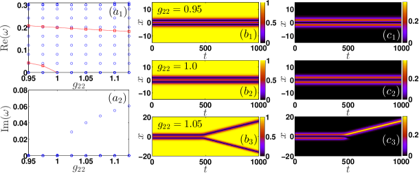
Figure 1: (Color online): BdG (linearization) spectrum of stationary antisymmetric two-DB soliton states, upon varying $g_{22}$. Both $(a_{1})$ the real, $\rm{Re}(\omega)$, and $(a_{2})$ the imaginary part, $\rm{Im}(\omega)$, of the eigenfrequencies $\omega$ are shown as a function of the intra-species repulsion $g_{22}$. Upon increasing $g_{22}$ there exists a critical value, $g_{22_{cr}}=1$, above which the antisymmetric branch destabilizes. Note that since $g_{12}=1$, the critical point is the integrable limit, while the trajectories of the two anomalous modes (see text) appearing in the spectrum are shown with red squares (solid red lines are used as a guide to the eye). $(b_{1})-(c_{3})$ Spatio-temporal evolution of antisymmetric stationary two-DB states upon increasing $g_{22}$, verifying the BdG results. $(b_{1})-(b_{3})$ [$(c_{1})-(c_{3})$] correspond to the density $|u_{d}|^{2}$ [$|u_{b}|^{2}$] of the dark [bright] component. All quantities are expressed in dimensionless units.

III Stability analysis of bound antisymmetric and asymmetric dark-bright pairs

By considering the time-independent version of the aforementioned system of Eqs. (3)-(4), namely:

$$u_{d} = -\frac{1}{2}\partial_{x}^{2}u_{d}+(|u_{d}|^{2}+g_{12}|u_{b}|^{2})u_{d},$$ (7)

$$\mu u_{b} = -\frac{1}{2}\partial_{x}^{2}u_{b}+(g_{12}|u_{d}|^{2}+g_{22}|u_{b}|^{2})u_{b},$$ (8)

bound states consisting of two DB solitons can be found in ljpp ; ljpp1 for out-of-phase or antisymmetric bright solitons for arbitrary nonlinear coefficients.

First, let us briefly recall what is known about the Manakov model. In such a case the system possesses exact two-DB soliton solutions that can be obtained by using either Hirota’s method studied in Ref. shepkiv or the more recent exact expressions found in Ref. prinari by using the inverse scattering transform (IST) but with non-trivial boundary conditions. In particular, the exact static two-DB solutions can be written in the following form:

$$u_{d} = \frac{(1-a)\cosh(\xi_{1}+\xi_{2})-(1+a)\cosh(\xi_{1}-\xi_{2})}{(1-a)\cosh(\xi_{1}+\xi_{2})+(1+a)\cosh(\xi_{1}-\xi_{2})},$$

$$u_{b} = \frac{2(1-a^{2})\sinh\xi_{1}}{(1-a)\cosh(\xi_{1}+\xi_{2})+(1+a)\cosh(\xi_{1}-\xi_{2})},$$

where $\xi_{1}=x-\delta_{1}$, $\xi_{2}=a(x-\delta_{2})$ and $\mu=1-a^{2}/2$.

There are three free parameters here: $a$, $\delta_{1}$ and $\delta_{2}$. One of them is due to the translational invariance: Shifting $\delta_{1}\rightarrow\delta_{1}+\bar{\delta}$, $\delta_{2}\rightarrow\delta_{2}+\bar{\delta}$ only displaces the overall solution by $\bar{\delta}$, so fixing the overall location of the pair one can fix $\delta_{1}=-\delta_{2}=:\delta$. Then one is still left with a nontrivial two-parameter family, with parameters $a$ and $\delta$. Fixing the chemical potential ratio $\mu$ fixes $a$ and vice versa (note that there is no loss of generality in assuming $a>0$ since $a\rightarrow-a$ only flips the global sign of $u_{d}$). The parameter $a$ must satisfy $0\leq a\leq 1$ and accordingly $1/2\leq\mu\leq 1$. The second parameter $\delta$ can also be taken positive since $\delta\rightarrow-\delta$, $x\rightarrow-x$ leaves $u_{d}$, $u_{b}$ invariant (up to a global sign), so changing the sign of $\delta$ just performs a reflection about $x=0$, exchanging the two DBs. For $\delta=0$, $u_{d}(x)=u_{d}(-x)$, $u_{b}(x)=-u_{b}(-x)$, so the DB pair is antisymmetric. As $\delta$ becomes larger, the asymmetry increases towards a dark/DB state and the equilibrium distance between the solitons increases. In our simulations $\mu$ is fixed, so $a$ is fixed. But still, in the integrable limit there will be a one-parameter family of two-DB solutions of varying $\delta$, continuously ranging from perfectly antisymmetric to extremely asymmetric.

As we depart from integrability, such an explicit expression is no longer available. In light of that, the corresponding stationary states were numerically obtained by means of a Newton’s fixed point iteration method and using as an initial guess for identifying the numerically exact (up to a prescribed tolerance) two-DB spatial profile the following ansatz:

$$\!\!\!\!\!\!u_{d}(x) = \tanh\left[D(x-x_{0})\right]\times\tanh\left[D(x+x_{0})\right],$$ (9)

$$\!\!\!\!\!\!u_{b}(x) = \eta{\rm sech}\left[D(x-x_{0})\right]+\eta{\rm sech}\left[D(x+x_{0})\right]e^{i\Delta\theta}.$$

In the above expressions $2x_{0}$ is the relative distance between the two DB solitons, $D$ denotes their common inverse width, while $\Delta\theta$ is their relative phase within the bright component, with $\Delta\theta=\pi$ ($\Delta\theta=0$) corresponding to out-of-phase (in-phase) bright solitons. Note also that the (background) amplitude of the dark soliton component is unity, while $\eta$ denotes the amplitude of the bright soliton counterpart. Here, we will solely focus on the out-of-phase or antisymmetric case (as the in-phase case does not produce a bound state pair in the homogeneous setting ljpp ). Upon varying $g_{12}$ typically within the interval $0.75\leqslant g_{12}\leqslant 1.5$, while keeping both $\mu=2/3$ and $g_{22}=0.95$ fixed, earlier numerical studies ljpp ; ljpp1 showcased that antisymmetric two-DB states exist as stable configurations only within a bounded interval of the inter-species repulsion coefficient $g_{12}$ limited by critical points both in the miscible and in the immiscible regime, associated with a supercritical and a subcritical pitchfork bifurcation respectively. Furthermore, new families of solutions consisting of mass imbalanced DB pairs, i.e. different amplitudes between the bright soliton constituents, were found to bifurcate through pitchfork bifurcations from the above obtained antisymmetric states.

However, by fixing $g_{22}\neq 1$ in these previous works it has not been possible to systematically approach the Manakov limit of $g_{12}=g_{22}=1$. To address this important special limit, and explore the effect of breaking the integrability, below we fix $g_{12}=1$ and perform a continuation in $g_{22}$, i.e., starting from $g_{22}=0.95$ (immiscible regime) up to $g_{22}=1$ and beyond, towards the miscible domain of interactions, considering the fate of both the antisymmetric and asymmetric bound states. Note also that for the numerical findings to be presented below the rescaled chemical potential is fixed to $\mu=0.7$ in the dimensionless units adopted herein. In Figs. 1 $(a_{1})-(a_{2})$ the linearization, or so-called Bogolyubov-de Gennes (BdG), spectrum of the antisymmetric bound pairs is shown as a function of the nonlinear coefficient $g_{22}$. This is obtained by expanding around an equilibrium configuration as follows:

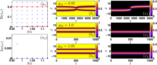
Figure 2: (Color online): $(a_{1})-(b_{2})$ Same as in Fig. 1 but for the asymmetric two-DB states. Notice that in contrast to the antisymmetric states, these bound pairs are unstable for $g_{22}<1$, as can be seen from the non-zero imaginary part, $\rm{Im}(\omega)$, depicted in panel $(a_{2})$. As the integrable limit is reached the bound pair stabilizes and remains robust even upon further increasing the nonlinear coefficient $g_{22}$. $(b_{1})-(c_{3})$ Space-time evolution of both the unstable ($g_{22}<1$) and stable ($g_{22}\geqslant 1$) asymmetric stationary two-DB states upon increasing $g_{22}$. Panels $(b_{1})-(b_{3})$ [$(c_{1})-(c_{3})$] correspond to the density $|u_{d}|^{2}$ [$|u_{b}|^{2}$] of the dark [bright] component. All quantities are expressed in dimensionless units.

$$u_{d} = u_{d}^{(eq)}+\left(a(x)e^{-i\omega t}+b^{\star}(x)e^{i\omega^{\star}t}\right),$$ (11)

$$u_{b} = u_{b}^{(eq)}+\left(c(x)e^{-i\omega t}+d^{\star}(x)e^{i\omega^{\star}t}\right),$$ (12)

where “$\star$” stands for the complex conjugate. Then the system for the eigenfrequencies $\omega$ (or equivalently eigenvalues $\lambda=i\omega$) and eigenfunctions $(a,b,c,d)^{T}$ is numerically solved. If modes with purely real eigenvalues (imaginary eigenfrequencies) or complex eigenvalues (and thus eigenfrequencies) are identified, the configuration is characterized as dynamically unstable. Moreover, there is a class of modes that bears the potential to lead to instabilities. These are the modes with negative so-called energy or Krein signature krein . The relevant quantity is defined as

$$K=\omega\int\Big{(}|a|^{2}-|b|^{2}+|c|^{2}-|d|^{2}\Big{)}dx,$$ (13)

and can be directly evaluated on the basis of the eigenvector $(a,b,c,d)^{T}$ and eigenfrequency $\omega$. Both the real, $\rm{Re}(\omega)$, and the imaginary, $\rm{Im}(\omega)$, parts of the eigenfrequencies $\omega$ are depicted in Figs. 1 $(a_{1})$ and $(a_{2})$ respectively. Notice that in close contact with our previous findings ljpp ; ljpp1 , two anomalous (namely, bearing negative Krein signature) modes appear in the linearization spectra and their trajectories are denoted with red squares [see Fig. 1 $(a_{1})$]. Among these modes, the higher-lying one is found to be related to the out-of-phase vibration of the bound DB pair ljpp . More importantly, the lower-lying anomalous mode is associated, through its eigenvector, with a symmetry breaking in the bright soliton component, resulting in mass imbalanced (with respect to their bright soliton counterpart) DB pairs that we will trace later on in the dynamics. In both cases the aforementioned findings can be identified by adding the corresponding eigenvector to the relevant antisymmetric DB solution. The background (continuous, in the limit of infinite domain) spectrum is also depicted in the same figure with blue circles. As it is observed, upon increasing $g_{22}$ towards the integrable limit the frequencies of both of the anomalous modes decrease. Following the lower-lying mode it becomes apparent that there exists a critical point $g_{22_{cr}}=1$ where this mode goes from linearly stable (for $g_{22}<g_{22_{cr}}$) to linearly unstable (for $g_{22}>g_{22_{cr}}$). Notice that exactly at the integrable limit this anomalous mode becomes neutrally stable, while past $g_{22_{cr}}=1$ it destabilizes as it is evident from the non-zero imaginary part presented in Fig. 1 $(a_{2})$.

To verify the stability analysis results presented above, the spatio-temporal evolution of both the stable and unstable antisymmetric DB pairs is computed and shown in Figs. 1 $(b_{1})-(c_{3})$. Notice that the antisymmetric configuration is only slightly modified as $g_{22}$ is increased over the interval considered. Minor differences, mostly in the amplitude of the bound pairs upon increasing $g_{22}$, can be inferred by inspecting the overall decrease of the norm of the bright component (see Fig. 3 below). Here, Figs. 1 $(b_{1})-(b_{3})$ [$(c_{1})-(c_{3})$] correspond to the density of the dark [bright] soliton component. In particular, in all cases we use as an initial condition the numerically obtained stationary states at selected values of $g_{22}$, i.e., below, at and above the associated critical point, and we numerically evolve the system of Eqs. (3)-(4) using a fourth order Runge-Kutta integrator. As anticipated from the aforementioned BdG outcome, for $g_{22}>g_{22_{cr}}=1$ the instability dynamically manifests itself via a dramatic mass redistribution between the bright soliton counterparts. The latter leads in turn to the splitting of the bound pair and results in asymmetric states with a dark and a DB soliton pair repelling one another and moving towards the boundaries (cf. also with the corresponding non-integrable cases in ljpp ; ljpp1 ).

We now explore the same diagnostics for the asymmetric DB bound pairs that are degenerate with the antisymmetric ones in the integrable limit. These stationary asymmetric states are once again numerically identified and their stability outcome is summarized in Fig. 2. As before, Fig. 2 $(a_{1})$ depicts the real part, $\rm{Re}(\omega)$, of the eigenfrequncies $\omega$ as a function of $g_{22}$, while Fig. 2 $(a_{2})$ shows the corresponding imaginary part, $\rm{Im}(\omega)$. In the real part of the spectrum the absence of the lower-lying anomalous mode is verified. Recall that the existence of this mode in the spectrum of the antisymmetric branch signalled the presence of the asymmetric branch of solutions [see Fig. 1 $(a_{1})$]. In contrast to the antisymmetric states investigated above, this family of solutions is unstable for $g_{22}<1$ as is evident in that regime by a non-zero imaginary eigenfrequency illustrated in Fig. 2 $(a_{2})$. On the other hand, the state remains spectrally stable for $g_{22}\geqslant 1$, and the formerly unstable mode, now becomes an anomalous one with a real eigenfrequency. It is important to note here, that the equilibrium distance is found to be larger for the asymmetric states when compared with the antisymmetric ones [compare e.g. Fig. 2 $(b_{2})$ with Fig. 1 $(b_{2})$]. The equilibrium distance also becomes larger for the asymmetric states upon increasing $g_{22}$, as can be deduced by more closely inspecting e.g. Figs. 2 $(b_{2})$ and $(b_{3})$. As before, our BdG results are confirmed via the long-time evolution of the stationary asymmetric states and are illustrated in Figs. 2 $(b_{1})-(c_{3})$. Once more, Figs. 2 $(b_{1})-(b_{3})$ depict the evolution of the density of the dark soliton component, while Figs. 2 $(c_{1})-(c_{3})$ illustrate the propagation of the density of the bright soliton counterpart. As it is expected, for values $g_{22_{cr}}<1$ instability sets in almost from the beginning of the dynamics, with the solitons featuring attraction, more pronounced in the dark soliton counterpart shown in Fig. 2 $(b_{1})$, which results in a collision event at intermediate time scales. However, and as anticipated for $g_{22}=g_{12}=1$ shown in Figs. 2 $(b_{2})$ and $(c_{2})$ solitons remain intact throughout the propagation, a result that holds as such even upon considering parameters beyond the integrable limit and on the miscible side depicted in Figs. 2 $(b_{3})$ and $(c_{3})$.

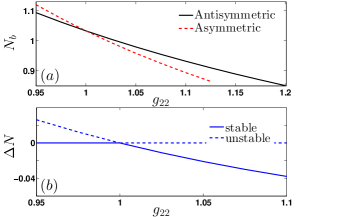
Figure 3: (Color online): $(a)$ Number of atoms, $N_{b}$, of the bright soliton components as a function of $g_{22}$ for both the antisymmetric and the asymmetric states. $(b)$ Transcritical bifurcation diagram obtained by measuring $\Delta N$ (see text) as a function of $g_{22}$. In all cases the stable (unstable) branches are denoted with solid (dashed) blue lines.

The above-observed differences between the antisymmetric and asymmetric branches of solutions can be further understood by inspecting the decrease in the number of atoms of the bright component, $N_{b}$, as a function of the nonlinear coefficient $g_{22}$ depicted for both cases in Fig. 3 $(a)$. It is observed that as $g_{22}$ increases the bright norm decreases faster for the asymmetric states, while the two norms are exactly the same at the integrable point. Finally, the transcritical nature of the bifurcation diagram is illustrated in Fig. 3 $(b)$. To obtain this bifurcation diagram we calculated the difference in the number of atoms in the bright part, $N_{b}$, for either the asymmetric or the antisymmetric branches of solutions defined as $\Delta N=N_{b}-N^{antisym.}_{b}$, upon varying the nonlinear coefficient $g_{22}$. Notice that the stability character of the antisymmetric and the asymmetric states is exchanged at the integrable point verifying the effectively transcritical nature of this bifurcation. It is worthwhile to comment a little on this bifurcation. Firstly, we point out that saddle-center and pitchfork examples are much more common than transcritical ones in our experience with Hamiltonian systems. In fact, the corresponding state where $\Delta N$ possesses the opposite sign (i.e., the parity symmetric variant of our DB-pair configuration) is also a solution. In that light, it can be thought of as transcritical bifurcation with symmetry. In fact, an even more crucial way in which the symmetry of the bifurcation can be appreciated is the neutrality discussed previously at the Manakov limit. The freedom in the variation of $\delta$ in that context represents a one-parameter family of solutions within which one can freely move and which represent different asymmetries in the bright component. A by-product of this invariance is the presence of a vanishing frequency eigenmode at the critical point of this bifurcation, i.e., at the transition point from stability to instability for the antisymmetric branch or vice-versa for the asymmetric one. However, it is important to point out that these features (neutrality, controllable asymmetry, and associated vanishing eigenfrequency) seem to disappear once we depart from the integrable limit, marking the absence of additional symmetry in the latter case.

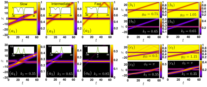
Figure 4: (Color online): $(a_{1})-(a_{6})$ Collisions between an initially at rest (i.e. $k_{1}=0$) DB pair and a moving one at the integrable limit. From left to right the velocity, $k_{2}$, of the moving DB pair is increased from $k_{2}=0.35$ to $k_{2}=0.85$, $\phi_{1}=\phi_{2}=\pi/4$, while the insets illustrate the initial profile of the two-DB state. Notice that as the velocity is increased the amplitude of the bright soliton decreases, leading, for $k_{2}=0.85$, to a state with almost only one bright soliton in the second component. $(b_{1})-(b_{4})$ The same as the above but for fixed $k_{2}=0.65$, and for different values of the intra-species repulsion. $(c_{1})-(c_{4})$ The same as before but upon varying the phase between the soliton constituents, namely for $\phi_{1}=0$ and $\phi_{2}=\pi$. In all cases the panels depict the density, $|q_{1}(x,t)|^{2}$, $\left(|q_{2}(x,t)|^{2}\right)$ of the dark (bright) soliton component in the top (bottom), while all quantities shown are in dimensionless units. Other parameters used are $\nu_{1}=0.8$, and $\nu_{2}=0.5$.

IV Dark-bright soliton collisions

In what follows we consider collisions between two-DB states at the integrable limit of equal inter- and intra-species interactions, i.e. $g_{12}=g_{22}=1$, as well as deviating from it towards the miscible and the immiscible regime. In both cases we use as an initial ansatz ($t=0$) the exact solution for such two-DB states, namely prinari ; biondini :

$$q_{1}(x,0) = q_{o}\Bigg{[}1+\frac{1}{D(x,0)}\Big{[}\bar{\delta}_{1}\frac{(z_{1}^{\star})^{2}}{q_{o}^{2}-z_{1}z_{2}}\left(\delta_{1}\frac{q_{o}^{2}-z_{1}z_{2}^{\star}}{z_{1}(z_{1}^{\star}-z_{1})}e^{-2\nu_{1}x}-\delta_{2}\frac{q_{o}^{2}-|z_{2}|^{2}}{z_{2}(z_{2}-z_{1}^{\star})}e^{ix(z_{2}-z_{1}^{\star})}\right)$$ (14)

$$+ \frac{\bar{\delta}_{2}(z_{2}^{\star})^{2}}{q_{o}^{2}-z_{1}z_{2}}\left(\delta_{2}\frac{q_{o}^{2}-z_{1}^{\star}z_{2}}{z_{2}(z_{2}^{\star}-z_{2})}e^{-2\nu_{2}x}-\delta_{1}\frac{q_{o}^{2}-|z_{1}|^{2}}{z_{1}(z_{1}-z_{2}^{\star})}e^{ix(z_{1}-z_{2}^{\star})}\right)$$

$$+ q_{o}^{4}|\delta_{1}|^{2}|\delta_{2}|^{2}\frac{\left(q_{o}^{2}-|z_{1}|^{2}\right)\left(q_{o}^{2}-|z_{2}|^{2}\right)|q_{o}^{2}-z_{1}^{\star}z_{2}|^{2}|z_{1}-z_{2}|^{4}\left(z_{1}^{\star}z_{2}^{\star}-z_{1}z_{2}\right)}{16\nu_{1}^{2}\nu_{2}^{2}z_{1}z_{2}|q_{o}^{2}-z_{1}z_{2}|^{2}|z_{1}^{\star}-z_{2}|^{4}}e^{-2x\left(\nu_{1}+\nu_{2}\right)}\Big{]}\Bigg{]},$$

$$\vspace{0.5cm}q_{2}(x,0) = -\frac{q_{o}}{D(x,0)}\Bigg{[}\frac{\bar{\delta}_{1}z_{1}^{\star}}{q_{o}^{2}}e^{-iz_{1}^{\star}x}+\frac{\bar{\delta}_{2}z_{2}^{\star}}{q_{o}^{2}}e^{-iz_{2}^{\star}x}+\Big{[}\frac{\bar{\delta}_{1}\bar{\delta}_{2}z_{1}^{\star}z_{2}^{\star}\left(q_{o}^{2}-z_{1}^{\star}z_{2}^{\star}\right)\left(z_{1}^{\star}-z_{2}^{\star}\right)^{2}}{q_{o}^{2}\left(q_{o}^{2}-z_{1}z_{2}\right)}\Big{]}$$ (15)

$$\times \Big{[}\frac{\delta_{1}z_{1}}{\left(z_{1}^{\star}-z_{1}\right)^{2}\left(z_{1}-z_{2}^{\star}\right)^{2}}e^{-2\nu_{1}x-iz_{2}^{\star}x}+\frac{\delta_{2}z_{2}}{(z_{2}^{\star}-z_{2})^{2}(z_{2}-z_{1}^{\star})^{2}}e^{-2\nu_{2}x-iz_{1}^{\star}x}\Big{]}\Bigg{]}.$$

Here, $q_{1}(x,0)$ [$q_{2}(x,0)$] is the wavefunction for the two dark [bright] soliton solution of the first [second] component in the system of Eqs. (LABEL:nls1)-(LABEL:nls2). $q_{o}$ is the amplitude of the background, $z_{j}=\kappa_{j}+i\nu_{j}$ correspond to the eigenvalues of the IST problem where $k_{j}=2\kappa_{j}$ is the soliton’s velocity, while $\delta_{j}$ are the so-called norming constants prinari ; biondini . In all cases $j=1,2$ accounts for the first and the second component of the vector nonlinear Schrödinger system. Additionally, $\bar{\delta}_{1}=-\delta_{1}^{\star}(q_{o}^{2}(q_{o}^{2}-|z_{1}|^{2})(q_{o}^{2}-z_{1}^{\star}z_{2}))/((z_{1}^{\star})^{2}(q_{o}^{2}-z_{1}^{\star}z_{2}^{\star}))$, and $\bar{\delta}_{2}=-\delta_{2}^{\star}(q_{o}^{2}(q_{o}^{2}-|z_{2}|^{2})(q_{o}^{2}-z_{2}^{\star}z_{1}))/((z_{2}^{\star})^{2}(q_{o}^{2}-z_{1}^{\star}z_{2}^{\star}))$, are related to the complex conjugates of the aforementioned norming constants. The denominator of the above equations is given by

$$D(x,0)=1 - \frac{\bar{\delta}_{1}(z_{1}^{\star})^{2}}{q_{o}^{2}-z_{1}z_{2}}\left(\delta_{1}\frac{q_{o}^{2}-z_{1}z_{2}^{\star}}{4\nu_{1}^{2}}e^{-2\nu_{1}x}-\delta_{2}\frac{q_{o}^{2}-|z_{2}|^{2}}{\left(z_{2}-z_{1}^{\star}\right)^{2}}e^{ix\left(z_{2}-z_{1}^{\star}\right)}\right)$$ (16)

$$+ \frac{\bar{\delta}_{2}(z_{2}^{\star})^{2}}{q_{o}^{2}-z_{1}z_{2}}\left(-\delta_{2}\frac{q_{o}^{2}-z_{2}z_{1}^{\star}}{4\nu_{2}^{2}}e^{-2\nu_{2}x}+\delta_{1}\frac{q_{o}^{2}-|z_{1}|^{2}}{\left(z_{1}-z_{2}^{\star}\right)^{2}}e^{ix(z_{1}-z_{2}^{\star})}\right)$$

$$+ q_{o}^{4}|\delta_{1}|^{2}|\delta_{2}|^{2}\frac{\left(q_{o}^{2}-|z_{1}|^{2}\right)\left(q_{o}^{2}-|z_{2}|^{2}\right)|q_{o}^{2}-z_{1}z_{2}^{\star}|^{2}|z_{1}-z_{2}|^{4}}{16\nu_{1}^{2}\nu_{2}^{2}|q_{o}^{2}-(z_{1}z_{2})|^{2}|z_{1}^{\star}-z_{2}|^{4}}e^{-2x\left(\nu_{1}+\nu_{2}\right)}.$$

Figure 5: (Color online): Collisions of DB states with zero initial velocities, $k_{1}=k_{2}=0$, and upon increasing $g_{22}$. The corresponding density profiles for $g_{22}=0.85$ are illustrated as insets in panels $(a_{1})$ and $(b_{1})$. Notice the breathing dynamics that the DB pairs undergo as the intra-species repulsion is increased. $(a_{1})-(a_{5})$ [$(b_{1})-(b_{5})$] Evolution of the density, $|q_{1}(x,t)|^{2}$ [$|q_{2}(x,t)|^{2}$], of the dark [bright] soliton component. Other parameters used are $\nu_{1}=1/2$, $\nu_{2}=1/3$, $\delta_{1}=1+i/5$, and $\delta_{2}=1-i/3$. All quantities shown are expressed in dimensionless units.

In order to initialize the dynamics we first render the two-DB states of Eqs. (14)-(15) well-separated. The latter can be achieved by parametrizing the norming constants $\delta_{j}$ ($j=1,2$) as: $\delta_{j}=(2\nu_{j}/(q_{o}\sqrt{q_{o}^{2}-z_{j}^{2}}))\exp(x_{j}+i\phi_{j})$ and varying the position offset $x_{j}$, and/or the phase $\phi_{j}$. Throughout this work, the amplitude of the background is fixed to $q_{o}=1$. In the case examples presented in Figs. 4 $(a_{1})-(a_{6})$, the DB pairs are located around $x_{1}\approx 0$ and $x_{2}\approx-10$ respectively. Furthermore, we fix the corresponding phases $\phi_{1}=\phi_{2}=\pi/4$, the velocity of the first DB pair $k_{1}=0$, and we vary $k_{2}$ within the interval [0.35, 0.85]. It is important to note that $k_{2}$ also significantly influences the asymmetry between the bright soliton counterparts. More specifically, for high speed solitons i.e., for $k_{2}>0.75$, the moving DB has a very weak bright component gradually becoming a single dark soliton impinging on a DB stationary wave. We have conducted numerous collisional simulations at and below as well as above the integrable limit (in terms of values of $g_{22}$). Our main finding in these cases where one of the solitons possesses a substantial speed is that generically the collisional phenomenology remains essentially similar [see also Figs. 4 $(b_{1})-(b_{4})$, as well as Figs. 4 $(c_{1})-(c_{4})$] to what is predicted by the analytical expressions of the integrable limit prinari .

This situation is in contrast to cases where the solitons have been initialized with vanishing speed, in which we have seen that the breaking of integrability has a maximal impact. A characteristic example of this kind is given in Figs. 5 $(a_{1})-(b_{5})$, where once more Figs. 5 $(a_{1})-(a_{5})$ [$(b_{1})-(b_{5})$] depict the breathing dynamics of the dark [bright] soliton constituent. In this case involving $k_{1}=k_{2}=0$, and the choice of the norming constants of $\delta_{1}=1+i/5$ and $\delta_{2}=1-i/3$ (for $\nu_{1}=1/2$ and $\nu_{2}=1/3$), we find that at the integrable limit the solution forms a beating state. This “fragile” beating is already seen to be significantly impacted by small deviations from integrability of the order of $5\%$ as it is evident in Figs. 5 $(a_{2}),(b_{2})$, and $(a_{4}),(b_{4})$, which refer to deviations towards the miscible and the immiscible regime respectively. However, the phenomenology is dramatically affected for deviations of the order of $15\%$ or more, whereby the former beating state gives way, upon already the first collision of the DB pair, to an indefinite separation between the two DBs. Remarkably, this deviation takes place both in the miscible, Figs. 5 $(a_{1}),(b_{1})$, and in the immiscible regime, Figs. 5 $(a_{5}),(b_{5})$. Under different values of the norming constants, the departure from the breathing state may be “decelerated”. A case example of this kind is depicted in Fig. 6. In particular in this realization all parameters used are the same as in the aforementioned collisional scenario except for $\delta_{1}=5+i/5$. Notice that for this choice of parameters the aforementioned deceleration against repulsion is more pronounced within the immiscible regime of interactions [compare e.g. panels $(a_{5})$ and $(b_{5})$ here, with Figs. 5 $(a_{5})$ and $(b_{5})$].

Figure 6: (Color online): Same as in Fig. 5 but for $\delta_{1}=5+i/5$, with all quantities shown expressed in dimensionless units.

Furthermore, this change in the norming constant affects the bright soliton characteristics resulting in particular in slightly mass imbalanced bright soliton counterparts, illustrated as insets in Figs. 6 $(a_{1})$ and $(b_{1})$, when compared to the spatial profiles of the solitons shown as insets in Figs. 5 $(a_{1})$ and $(b_{1})$. On the other hand, when initializing the dynamics considering a genuinely stationary configuration, the results of the stability analysis of the previous section are confirmed. Namely, for a genuinely antisymmetric bright configuration, stability persists on the side of $g_{22}<1$, while a splitting (symmetry breaking) instability into a DB and a dark soliton arises for $g_{22}>1$, with the stability intervals being reversed for asymmetric initial conditions.

V Conclusions and future challenges

In the present work we have investigated the stability and dynamics of matter-wave DB solitons in homogeneous binary BECs. We have done so by taking advantage in a systematic fashion of the understanding and knowledge imparted by the inverse scattering transform and the Hirota method within the integrable Manakov limit. In that limit, both antisymmetric and asymmetric DB pair waveforms are identified, but also solutions involving DB pairs interacting with different speeds can be explored via cumbersome, yet explicit analytically available formulae. We have benchmarked the results of our numerical simulations against these expressions and subsequently extended our analysis past the integrable limit to identify the nature of the deviations from the corresponding results. This has given rise to an array of interesting findings. In particular, in the case of stationary solutions we have identified an intriguing transcritical bifurcation with symmetry. Antisymmetric and asymmetric solutions in the bright soliton component of the DB pairs have been found, respectively to be, stable (unstable) for $g_{22}<1$ ($g_{22}>1$), exchanging their stability in the degenerate (invariant under symmetry breaking) case of the integrable limit. Moreover, as regards collisions, we have seen that those bearing significant kinetic energy were essentially unaffected by the breaking of integrability. On the other hand, the more delicate beating (or even stationary) states were drastically affected by the breaking of integrability, typically leading to the fission of the elements within the pair, possibly accompanied by a symmetry breaking between the bright components.

These findings suggest a multitude of interesting directions for future studies. A straight forward one would be to consider such multicomponent interactions in the presence of quantum fluctuations lgs . In such a setting it has recently been shown that DB states decay into daughter DB ones, so it would be particularly interesting to explore how the collisional dynamics of the above beating states is altered by taking into account beyond mean-field effects. Yet another interesting aspect would be to extend our current considerations involving a higher number of species. In this spinor setting, solutions in the form of dark-dark-bright and dark-bright-bright solitons have been theoretically obtained BG , and also very recently experimentally observed PGK_Engels . Thus a study of their static and dynamical properties will enhance our understanding of these soliton complexes. Furthermore, one could also explore multicomponent interactions as the ones considered herein but in higher dimensions. As is well-known there are no direct analogues of the Manakov model that are known to be integrable at present. However, it is nevertheless of interest to explore interactions of vortex-bright solitons in two dimensions pola and of configurations such as vortex line-bright solitons or vortex-ring-bright solitons in three dimensions wenlong . These possibilities are presently under consideration and will be reported in future publications.

References

- (1) L. P. Pitaevskii, and S. Stringari, Bose-Einstein Condensation, Oxford University Press, (Oxford, 2003).
- (2) P. G. Kevrekidis, D. J. Frantzeskakis, and R. Carretero-González, Emergent Nonlinear Phenomena in Bose-Einstein Condensates, Springer-Verlag (Berlin, 2008).
- (3) P. G. Kevrekidis, and D. J. Frantzeskakis, Reviews in Physics 1, 140 (2016).
- (4) C. Becker, S. Stellmer, P. Soltan-Panahi, S. Dörscher, M. Baumert, E.-M. Richter, J. Kronjäger, K. Bongs, and K. Sengstock, Nat. Phys. 4, 496 (2008).
- (5) D. Yan, J. J. Chang, C. Hamner, P. G. Kevrekidis, P. Engels, V. Achilleos, D. J. Frantzeskakis, R. Carretero-González, P. Schmelcher, Phys. Rev. A 84, 053630 (2011).
- (6) T. Busch, and J. R. Anglin, Phys. Rev. Lett. 87, 010401 (2001).
- (7) C. J. Hamner, J. J. Chang, P. Engels, and M. A. Hoefer, Phys. Rev. Lett. 106, 065302 (2011).
- (8) S. Middelkamp, J. J. Chang, C. Hamner, R. Carretero-González, P. G. Kevrekidis, V. Achilleos, D. J. Frantzeskakis, P. Schmelcher, and P. Engels, Phys. Lett. A 375, 642 (2011).
- (9) A. Álvarez, J. Cuevas, F. R. Romero, C. Hamner, J. J. Chang, P. Engels, P. G. Kevrekidis, and D. J. Frantzeskakis, J. Phys. B 46, 065302 (2013).
- (10) M. J. Ablowitz, B. Prinari, and A. D. Trubatch, Discrete and Continuous Nonlinear Schrödinger Systems, Cambridge University Press (Cambridge, 2004).
- (11) P. G. Kevrekidis, D. J. Frantzeskakis, and R. Carretero-González, The Defocusing Nonlinear Schrödinger Equation, SIAM (Philadelphia, 2015).
- (12) S. V. Manakov, Zh. Eksp. Teor. Fiz. 65, 505 (1973) [Sov. Phys. JETP 38, 248 (1974)].
- (13) D. Garrett, T. Klotz, B. Prinari, and F. Vitale, Applic. Anal. 92, 379 (2013).
- (14) B. Prinari, F. Vitale, and G. Biondini, J. Math. Phys. 56, 071505 (2015).
- (15) A. P. Sheppard, and Yu. S. Kivshar, Phys. Rev. E 55, 4773 (1997).
- (16) V. V. Afanasjev, Yu. S. Kivshar, V. V. Konotop, and V. N. Serkin, Opt. Lett. 14, 805 (1989).
- (17) R. Radhakrishnan, and M. Lakshmanan, J. Phys. A: Math. Gen. 28, 2683 (1995).
- (18) Q. -H. Park and H. J. Shin, Phys. Rev. E 61, 3093 (2000).
- (19) S. Rajendran, P. Muruganandam, and M. Lakshmanan, J. Phys. B 42, 145307 (2009).
- (20) S. Inouye, M. R. Andrews, J. Stenger, H.-J. Miesner D. M. Stamper-Kurn, and W. Ketterle, Nature (London) 392, 151 (1998).
- (21) J. L. Roberts, N. R. Claussen, J. P. Burke, Jr., C. H. Greene, E. A. Cornell, and C. E. Wieman, Phys. Rev. Lett. 81, 5109 (1998).
- (22) E. A. Donley, N. R. Claussen, S. L. Cornish, J. L. Roberts, E. A. Cornell, and C. E. Wieman, Nature (London) 412, 295 (2001).
- (23) G. Thalhammer, G. Barontini, L. de Sarlo, J. Catani, F. Minardi, and M. Inguscio, Phys. Rev. Lett. 100, 210402 (2008).
- (24) C. Chin, R. Grimm, P. Julienne, and E. Tiesinga, Rev. Mod. Phys. 82, 1225 (2010).
- (25) D. Yan, F. Tsitoura, P. G. Kevrekidis, and D. J. Frantzeskakis, Phys. Rev. A 91, 023619 (2015).
- (26) E. T. Karamatskos, J. Stockhofe, P. G. Kevrekidis, and P. Schmelcher, Phys. Rev. A 91, 043637 (2015).
- (27) G. C. Katsimiga, J. Stockhofe, P. G. Kevrekidis, and P. Schmelcher, Phys. Rev. A 95, 013621 (2017).
- (28) O. Majed, D. Alotaibi, and L. D. Carr, Phys. Rev. A 96, 013601 (2017).
- (29) G. C. Katsimiga, J. Stockhofe, P. G. Kevrekidis, and P. Schmelcher, Appl. Sci. 7, 388 (2017).
- (30) P. Ao, and S. T. Chui, Phys. Rev. A 58, 4836 (1998).
- (31) D. V. Skryabin, Phys. Rev. A 63, 013602 (2000).
- (32) G. C. Katsimiga, G. M. Koutentakis, S. I. Mistakidis, P. G. Kevrekidis, and P. Schmelcher, New J. Phys. 19 073004 (2017).
- (33) G. Biondini, D. K. Kraus, and B. Prinari, Commun. Math. Phys. 348, 475 (2016).
- (34) T. M. Bersano, V. Gokhroo, M. A. Khamehchi, J. D’ Ambroise, D. J. Frantzeskakis, P. Engels, and P. G. Kevrekidis, arXiv:1705.08130 (2017).
- (35) M. Pola, J. Stockhofe, P. Schmelcher, and P. G. Kevrekidis, Phys. Rev. A 86, 053601 (2012).
- (36) E. G. Charalampidis, W. Wang, P. G. Kevrekidis, D. J. Frantzeskakis, and J. Cuevas-Maraver, Phys. Rev. A 93, 063623 (2016).