Abstract

There is a recent surge of interest in nonconvex reformulations via low-rank factorization for stochastic convex semidefinite optimization problem in the purpose of efficiency and scalability. Compared with the original convex formulations, the nonconvex ones typically involve much fewer variables, allowing them to scale to scenarios with millions of variables. However, it opens a new challenge that under what conditions the nonconvex stochastic algorithms may find the global optima effectively despite their empirical success in applications. In this paper, we provide an answer that a stochastic gradient descent method with variance reduction, can be adapted to solve the nonconvex reformulation of the original convex problem, with a global linear convergence, i.e., converging to a global optimum exponentially fast, at a proper initial choice in the restricted strongly convex case. Experimental studies on both simulation and real-world applications on ordinal embedding are provided to show the effectiveness of the proposed algorithms.

1 Introduction

The stochastic convex semidefinite optimization problem, arising in many applications like non-metric multidimensional scaling [1, 6], matrix sensing [12, 22], community detection [14], synchronization [4], and phase retrieval [10], is of the following form:

$$\mathop{\mathrm{min}}_{X\in\mathbb{R}^{p\times p}}\ f(X)=\frac{1}{n}\sum_{i=1}^{n}f_{i}(X)\quad\mathrm{s.t.}\quad X\succeq 0,$$ (1)

where $f_{i}(X)$ is some convex, smooth cost function associated with the $i$-th sample, $X\succeq 0$ is the positive semidefinite (PSD) constraint.

There are many algorithms for solving problem (1), mainly including the first-order methods like the well-known projected gradient descent method [17], interior point method [2], and more specialized path-following interior point methods which use the (preconditioned) conjugate gradient or residual scheme to compute the Newton direction (for more detail, see the survey [15] and references therein). However, most of these methods are not well-scalable due to the PSD constraint, i.e., $X\succeq 0$. To circumvent this difficult constraint, the idea of low-rank factorization was adopted in literature [8, 9] and became very popular in the past few years due to its empirical success [5]. Low-rank factorization recasts the original problem (1) into an unconstrained problem by introducing another rectangular matrix $U\in\mathbb{R}^{p\times r}$ with $r<p$ such that $X=UU^{T}$. Let $g(U):=f(UU^{T})$ and problem (1) leads to,

$$\mathop{\mathrm{min}}_{U\in\mathbb{R}^{p\times r}}\ g(U)\quad\mathrm{where}\quad r\leq p.$$ (2)

Problems (1) and (2) will be equivalent when $r\geq r^{*}$ in the sense that problem (2) can find a global optimum $X^{*}$ of problem (1) with $r^{*}=\mathrm{rank}(X^{*})$. Since the PSD constraint has been eliminated, the recast problem (2) has a significant advantage over (1), but this benefit has a corresponding cost: the objective function is no longer convex but instead nonconvex in general. Even for the simple first-order methods like the factored gradient descent (FGD), its global linear convergence remains unspecified until a recent work in [5]. Moreover, facing the challenge in large scale applications with a big $n$, stochastic algorithms [19] have been widely adopted nowadays, that is, at each iteration, we only use the gradient information of one or a small batch of the whole sample instead of the full gradient over $n$ samples. However, due to the variance of such stochastic gradients, the stochastic gradient descent (SGD) method only has a sublinear convergence rate even in the strongly convex case. Various variance reduction techniques have been proposed in literature (see, e.g., [13, 20]), which resume the linear convergence for strongly convex problems. However, it is still open whether these methods can be adapted to the nonconvex problem (2) while enjoying the linear convergence to global optima.

The main contribution in this paper is to fill in this gap by showing that, when adapted to the nonconvex problem (2), our proposed versions of stochastic variance reduced gradient (SVRG) method can find the global optimum of the original problem (1) at a linear convergence rate when the initial choice lies in a prescribed neighbour of the global optimum and the objective function is restricted strongly convex. The initial choice condition here improves the one proposed for FGD in [5]. Moreover, our proposal includes both the fixed step sizes and the adaptive ones using a stabilized modification of Barzilai-Borwein (BB) step sizes [3] which adapts to the non-convex problems when the curvature is not guaranteed as in strongly convex cases. Finally, experiments on both matrix sensing and ordinal embedding demonstrate the effectiveness of the proposed scheme.

The reminder of this paper is organized as follows. Section 2 introduce some algorithmic background with our proposal. Section 3 presents the main convergence results. Section 4 provides some initialization schemes. Section Supplementary Material: Proofs outlines the proof of our main theorem. Section 6 provides some applications to verify our theoretical findings and show the effectiveness of the proposed algorithms. We conclude this paper in Section 7.

Notations: For any two matrices $X,Y\in\mathbb{R}^{p\times p}$, their inner product is defined as $\langle X,Y\rangle=\mathrm{tr}(X^{T}Y)$. We denote $\mathbb{S}_{+}^{p}$ as the set of positive semidefinite matrices of size $p\times p$. For any matrix $X\in\mathbb{R}^{p\times p}$, $\|X\|_{F}$ and $\|X\|_{2}$ denote its Frobenius and spectral norms, respectively, and $\sigma_{\min}(X)$ and $\sigma_{\max}(X)$ denote the smallest and largest strictly positive singular values of $X$, denote $\tau(X):=\frac{\sigma_{\max}(X)}{\sigma_{\min}(X)}$, with a slight abuse of notation, we also use $\sigma_{1}(X)\equiv\sigma_{\max}(X)\equiv\|X\|_{2}$, and $X_{r}$ denotes the rank-$r$ approximation of $X$ via its truncated singular value decomposition (SVD) for any $r\leq p$. ${\bf I}_{p}$ denotes the identity matrix with the size $p\times p$. We will omit the subscript $p$ of ${\bf I}_{p}$ if there is no confusion in the context.

2 Algorithms

  Parameters: update frequency $m$, step size (or learning rate) $\{\eta_{k}\}$, initial point $\tilde{U}^{0}\in\mathbb{R}^{p\times r}$

  for k=0,1,… do

     $\tilde{X}^{k}:=\tilde{U}^{k}{(\tilde{U}^{k})}^{T}$

     $g_{k}=\frac{1}{n}\sum_{i=1}^{n}\nabla f_{i}(\tilde{X}^{k})\tilde{U}^{k}$

     $U^{0}=\tilde{U}^{k}$

     for $t=0,\ldots,m-1$ do

        $X^{t}=U^{t}{U^{t}}^{T}$

        Randomly pick $i_{t}\in\{1,\ldots,n\}$

        $U^{t+1}=U^{t}-\eta_{k}(\nabla f_{i_{t}}(X^{t})U^{t}-\nabla f_{i_{t}}(\tilde{X}^{k})\tilde{U}^{k}+g_{k})$

     end for

     $\tilde{U}^{k+1}=U^{m}$

  end for

Algorithm 1 SVRG for Problem (1)

Without loss of generality, we assume that $f$ is a symmetric function, i.e., $f(X)=f(X^{T})$ throughout the paper. For $X=UU^{T}$, the gradient of $g(U):=f(UU^{T})$ is

$$\nabla g(U)=(\nabla f(UU^{T})+\nabla f(UU^{T})^{T})U=2\nabla f(X)U.$$

A. FGD: The FGD method proposed by [5] can be described as follows: let $U^{t}$ be the iterate at the $t$-th iteration and $X^{t}:=U^{t}{U^{t}}^{T}$, then the next iterate $U^{t+1}$ is updated according to the following

$$U^{t+1}=U^{t}-\eta\nabla f(X^{t})U^{t},$$ (3)

where $\eta>0$ is a step size.

B. Stochastic FGD (SFGD): As a stochastic counterpart of FGD (3), SFGD here can be naturally described as follows: at the $t$-th iteration, randomly pick an $i_{t}\in\{1,\ldots,n\}$, then update the next iteration via

$$U^{t+1}=U^{t}-\eta_{t}\nabla f_{i_{t}}(X^{t})U^{t},$$ (4)

where $\eta_{t}>0$ is a diminishing step size.

C. SVRG: The SVRG method was firstly proposed by [13] for minimizing a finite sum of convex functions with a vector argument. The main idea of SVRG is adopting the variance reduction technique to accelerate SGD and achieve the linear convergence rate. Specifically, SVRG for solving problem (2) can be described as in Algorithm 1. There are mainly two loops including an inner loop and an outer loop in SVRG. One important implementation issue of SVRG is the tuning of the step size. There are mainly two classes of step sizes: determined or data adaptive. Here we discuss three particular choices.

1. Fixed step size [13]:

   $$\eta_{k}\equiv\eta,\quad\text{for some}\ \eta>0.$$ (5)

2. Barzilai-Borwein (BB) step size [3, 21]: given an initial $\eta_{0}>0$ and for $k\geq 1$, let $\tilde{g}_{k}:=\nabla f(\tilde{X}^{k})$,

   $$\eta_{k}=\frac{1}{m}\cdot\frac{\|\tilde{X}^{k}-\tilde{X}^{k-1}\|_{F}^{2}}{|\langle\tilde{X}^{k}-\tilde{X}^{k-1},\tilde{g}_{k}-\tilde{g}_{k-1}\rangle|}.$$ (6)

   Note that such a BB step size is originally studied for strongly convex objective functions [21], and it may be breakout if there is no guarantee of the curvature of $f$ like in nonconvex cases. In order to avoid such possible instability of (6) in our studies, a variant of BB step size, called the stabilized BB step size, is suggested as follows.

3. Stabilized BB (SBB) step size: given an initial $\eta_{0}>0$ and an $\epsilon\geq 0$, for $k\geq 1$,

   $$\eta_{k}=\frac{1}{m}\times$$ (7)

   $$\frac{\|\tilde{X}^{k}-\tilde{X}^{k-1}\|_{F}^{2}}{|\langle\tilde{X}^{k}-\tilde{X}^{k-1},\tilde{g}_{k}-\tilde{g}_{k-1}\rangle|+\epsilon\|\tilde{X}^{k}-\tilde{X}^{k-1}\|_{F}^{2}}.$$

Throughout the rest of paper, with a slight abuse, we still name the original SVRG with a fixed step size as SVRG, and call the SVRG with stabilized BB step size (7) as SVRG-SBB_ϵ, and particularly, we call SVRG with BB step size as SVRG-SBB₀. Besides the above three step sizes, there are some other schemes like the diminishing step size and the use of smoothing technique in BB step size as discussed in [21]. However, we mainly focus on the listed three step sizes in this paper due to they have been demonstrated to be effective in practice. Moreover, we only consider the Option-I suggested in [13] for Algorithm 1, since Option-I in SVRG is generally a more natural and better choice than Option-II as demonstrated in both [13] and [21] in the vector setting.

3 Global Linear Convergence of SVRGs

To present our main convergence results, we need the following assumptions.

Assumption 1

Each $f_{i}$ ($i=1,\ldots,n$) satisfies the following:

1. $f_{i}$ is $L$-Lipschitz differentiable for some constant $L>0$, i.e., $f_{i}$ is smooth and $\nabla f_{i}$ is Lipschitz continuous satisfying

   $$\|\nabla f_{i}(X)-\nabla f_{i}(Y)\|_{F}\leq L\|X-Y\|_{F},\ \forall X,Y\in\mathbb{S}_{+}^{p}.$$

2. $f_{i}$ is $(\mu,r)$-restricted strongly convex for some constants $\mu>0$ and $r\leq p$, i.e., for any $X,Y\in\mathbb{S}_{+}^{p}$ with rank-$r$

   $$f_{i}(Y)\geq f_{i}(X)+\langle\nabla f_{i}(X),Y-X\rangle+\frac{\mu}{2}\|Y-X\|_{F}^{2}.$$

Assumption 1 implies that $f$ is also $L$-Lipschitz differentiable and $(\mu,r)$-restricted strongly convex. For any $L$-Lipschitz differentiable and $(\mu,r)$-restricted strongly convex function $h$, the following hold ([18])

$$h(Y)\leq h(X)+\langle\nabla h(X),Y-X\rangle+\frac{L}{2}\|Y-X\|_{F}^{2},$$

$$\mu\|X-Y\|_{F}^{2}$$

$$\leq\langle\nabla h(X)-\nabla h(Y),X-Y\rangle\leq L\|X-Y\|_{F}^{2},$$

where the first inequality holds for any $X,Y\in\mathbb{S}_{+}^{p}$, and the second inequality holds for any $X,Y\in\mathbb{S}_{+}^{p}$ with rank $r$, the first inequality and the right-hand side of the second inequality hold for the Lipschitz continuity of $\nabla h$, and the left-hand side of the second inequality is due to the $(\mu,r)$-restricted strong convexity of $h$.

Let $X^{*}$ be a global optimum of problem (1) with rank $r^{*}:=\mathrm{rank}(X^{*})$, $X_{r}^{*}$ be its rank-$r$ ($r\leq r^{*}$) best approximation via truncated singular value decomposition (SVD), and $U_{r}^{*}$ be a decomposition of $X_{r}^{*}$ via $X_{r}^{*}=U_{r}^{*}{U_{r}^{*}}^{T}$. Under Assumption 1, we define the following constants:

$$\kappa:=\frac{L}{\mu},\quad\gamma_{0}:=\frac{2(\sqrt{2}-1)}{3\kappa},$$ (8)

$$\bar{\eta}:=\min\left\{\frac{(1-\sqrt{\gamma_{0}})^{2}}{\frac{\|\nabla f(X_{r}^{*})\|_{F}}{L\sigma_{r}(X_{r}^{*})}+(2\sqrt{\gamma_{0}}+\gamma_{0})\tau(U_{r}^{*})},1\right\},$$ (9)

$$\xi:=\bar{\eta}(1-\bar{\eta}/2),$$ (10)

where $\tau(X_{r}^{*}):=\frac{\sigma_{1}(X_{r}^{*})}{\sigma_{r}(X_{r}^{*})}$ and $\tau(U_{r}^{*}):=\frac{\sigma_{1}(U_{r}^{*})}{\sigma_{r}(U_{r}^{*})}$. $\kappa\geq 1$ is generally called the condition number of the objective function. Thus, $0<\gamma_{0}\leq\frac{2(\sqrt{2}-1)}{3}$ and $0<\xi\leq 1/2.$

As $r$ is used in the alternative nonconvex problem (2), the sequence $\{\tilde{X}^{k}\}$ generated by SVRG in Algorithm 1 is at least rank-$r$, and can only converge to a rank-$r$ matrix if it is convergent. Therefore, we impose the following assumption to guarantee that the distance between $X_{r}^{*}$ and $X^{*}$ should be relatively small, otherwise, the introduced problem (2) is not a good alterative of the original problem (1).

Assumption 2 (rank-$r$ approximation error)

Let $X^{*}$ be a global optimum of problem (1), $X_{r}^{*}$ be the rank-$r$ approximation of $X^{*}$ for a given positive integer $r\leq r^{*}:=\mathrm{rank}(X^{*})$. The following holds

$$\|X_{r}^{*}-X^{*}\|_{F}<\frac{\sqrt{2}-1}{\sqrt{3}}\xi^{1/2}\kappa^{-1}\cdot\sigma_{r}(X^{*}),$$

where $\kappa$ is specified in (8), and $\sigma_{r}(X^{*})$ is the $r$-th largest singular value of $X^{*}$.

Assumption 2 is a regular assumption used in literature (say, [5]). Roughly speaking, Assumption 2 can be regarded as some noise assumption on problem (1). On the other hand, Assumption 2 is imposed to guarantee the uniqueness of the rank-$r$ best approximation $X_{r}^{*}$. Otherwise, when $\|X_{r}^{*}-X^{*}\|_{F}\geq\sigma_{r}(X^{*})$, if $X^{*}={\bf I}_{5}$, i.e., an identity matrix with the size $5\times 5$, then $X_{r}^{*}$ with $r=4$ has five possible candidates. Such assumption naturally holds for $r=r^{*}$, and when $r<r^{*}$, it might be satisfied if the singular values of $X^{*}$ possess certain compressible property. Under Assumption 2, we define several positive constants as follows: $\Delta:=\frac{(\sqrt{2}-1)^{2}\xi^{2}\sigma_{r}^{2}(X_{r}^{*})}{3\kappa^{2}}-\xi\|X_{r}^{*}-X^{*}\|_{F}^{2},$ $\tilde{\Delta}:=\frac{4(\sqrt{2}-1)^{2}\xi^{2}\sigma_{r}^{2}(X_{r}^{*})}{9\kappa^{2}}-\xi\|X_{r}^{*}-X^{*}\|_{F}^{2},$

$$\gamma_{l}:=\frac{2(\sqrt{2}-1)\xi\sigma_{r}(X_{r}^{*})}{3\kappa}-\sqrt{\Delta},$$ (11)

$$\gamma_{u}:=\frac{2(\sqrt{2}-1)\xi\sigma_{r}(X_{r}^{*})}{3\kappa}+\sqrt{\Delta},$$ (12)

$$\tilde{\gamma}_{l}:=\frac{2(\sqrt{2}-1)\xi\sigma_{r}(X_{r}^{*})}{3\kappa}-\sqrt{\tilde{\Delta}},$$ (13)

$$\tilde{\gamma}_{u}:=\frac{2(\sqrt{2}-1)\xi\sigma_{r}(X_{r}^{*})}{3\kappa}+\sqrt{\tilde{\Delta}}.$$ (14)

Note that the following relations hold

$$\gamma_{l}+\gamma_{u}=\frac{4(\sqrt{2}-1)\xi\sigma_{r}(X_{r}^{*})}{3\kappa},$$ (15)

$$\tilde{\gamma}_{l}<\gamma_{l}<\gamma_{u}<\tilde{\gamma}_{u}\leq\gamma_{0}\sigma_{r}(X_{r}^{*}),$$ (16)

where the last inequality of (16) holds for $0<\xi\leq 1/2$ and $\tilde{\gamma}_{u}\leq 2\xi\gamma_{0}\sigma_{r}(X_{r}^{*})\leq\gamma_{0}\sigma_{r}(X_{r}^{*})$.

We also need the following common assumption on the stochastic direction, which has been widely used in literature on stochastic algorithms (say, [7] and reference therein).

Assumption 3 (Unbiasedness)

$\{\nabla f_{i_{t}}(X^{t})U^{t}\}$ satisfies $\mathbb{E}_{i_{t}}[\nabla f_{i_{t}}(X^{t})U^{t}]=\nabla f(X^{t})U^{t},\ \forall t\in\mathbb{N}$.

If $i_{t}$ is uniformly sampled, (see [16, 24] for studies on importance sampling), then the above assumption can be satisfied. Under Assumptions 1-3, let ${\cal N}_{\gamma_{0}}:=\{U:\|U-U_{r}^{*}\|^{2}_{F}\leq\gamma_{0}\sigma_{r}(X_{r}^{*})\}$, and we define the following constants: ${\cal B}:=\sup_{U\in{\cal N}_{\gamma_{0}}}\|UU^{T}\|_{F},$ $B_{0}:=\sup_{U\in{\cal N}_{\gamma_{0}}}\left\{\mathbb{E}_{i_{t}}[\|\nabla f_{i_{t}}(UU^{T})\|_{F}^{2}]-\|\nabla f(UU^{T})\|_{F}^{2}\right\},$ $B_{1}:=\sup_{U\in{\cal N}_{\gamma_{0}}}\|\nabla f(UU^{T})\|^{2}_{F},$

$$B_{2}:=4\left[2L^{2}{\cal B}({\cal B}+\|X_{r}^{*}\|_{F})+B_{0}+B_{1}\right],$$ (17)

$$\theta:=\frac{2\xi B_{2}}{L(\sqrt{\tilde{\Delta}}-\sqrt{\Delta})}=\frac{18B_{2}\kappa\delta}{(\sqrt{2}-1)^{2}\xi\mu\sigma_{r}^{2}(X_{r}^{*})},$$ (18)

$$\eta_{\max}:=\min\left\{\zeta_{1},\zeta_{2},\frac{1}{2\theta}\right\},$$ (19)

where $\delta:=\sqrt{\tilde{\Delta}}+\sqrt{\Delta},$ $\zeta_{1}:=\frac{1}{12\left[2L\cdot\kappa{\cal B}+\frac{B_{0}+B_{1}}{(\sqrt{2}-1)\mu\sigma_{r}(X_{r}^{*})}\right]},$ and $\zeta_{2}:=\frac{(\sqrt{2}-1)\mu\xi\sigma_{r}(X_{r}^{*})}{12B_{2}}$. It can be seen that ${\cal B}$ is the upper bound of $X=UU^{T}$, $B_{0}$ represents variance of the stochastic gradient of $f$, and $B_{1}$ is the upper bound of the squared Frobenius norm of gradient $\nabla f(UU^{T})$, restricted to the closed ball ${\cal N}_{\gamma_{0}}$.

Let $\{\eta_{k}\}$ be a sequence satisfying $\eta_{k}\in(0,\eta_{\max})$ for any $k\in\mathbb{N}$. Given a positive integer $m$, define

$$\rho_{k}:=1-\frac{\eta_{k}(\sqrt{2}-1)^{2}\xi\mu\sigma_{r}^{2}(X_{r}^{*})}{18\kappa\delta},$$ (20)

$$\tilde{\rho}_{k}:=\rho_{k}^{m}+(1-\rho_{k}^{m})\eta_{k}\theta.$$ (21)

It is easy to check that $0<\rho_{k}<1$ and $0<\tilde{\rho}_{k}<1$. Based on the above defined constants, we present our main theorem as follows.

Theorem 1 (Linear convergence of SVRG)

Let $\{\tilde{U}^{k}\}$ be a sequence generated by Algorithm 1. Suppose that Assumptions 1-3 hold, and that $\eta_{k}\in(0,\eta_{\max})$. The following hold: (a) if $\gamma_{l}<\|\tilde{U}^{0}-U_{r}^{*}\|_{F}^{2}<\gamma_{u},$ there hold

1. $\{\mathbb{E}[\|\tilde{U}^{k}-U_{r}^{*}\|_{F}^{2}]\}$ is monotonically decreasing,

2. (Linear convergence) for any $k\geq 1,$

   $$\mathbb{E}[\|\tilde{U}^{k}-U_{r}^{*}\|_{F}^{2}]$$ (22)

   $$\leq\left(\prod_{i=0}^{k-1}\tilde{\rho}_{i}\right)\cdot\|\tilde{U}^{0}-U_{r}^{*}\|_{F}^{2}+\tilde{\gamma_{l}}\times$$

   $$\left[\sum_{t=0}^{k-2}\left(\prod_{i=t+1}^{k-1}\tilde{\rho_{i}}\cdot(1-(\rho_{t})^{m})\right)+\left(1-(\rho_{k-1})^{m}\right)\right].$$

(b) In addition, if $\|\tilde{U}^{0}-U_{r}^{*}\|^{2}_{F}\leq\gamma_{l}$, then $\mathbb{E}[\|\tilde{U}^{k}-U_{r}^{*}\|_{F}^{2}]\leq\gamma_{l}$ for any $k\in\mathbb{N}$.

The above theorem holds for a generic step size satisfying $\eta_{k}\in(0,\eta_{\max})$. Actually, if $\{\eta_{k}\}$ is lower bounded by a positive constant $\eta_{\min}$ and obviously, $\eta_{\min}<\eta_{\max}$, then by (20) and (21), $\rho_{k}\in(\rho_{\min},\rho_{\max})$ and $\tilde{\rho}_{k}\in(\theta\eta_{\min},\tilde{\rho}_{\max}),$ where $\rho_{\min}:=1-\frac{\eta_{\max}(\sqrt{2}-1)^{2}\xi\mu\sigma_{r}^{2}(X_{r}^{*})}{18\kappa\delta}$, $\rho_{\max}:=1-\frac{\eta_{\min}(\sqrt{2}-1)^{2}\xi\mu\sigma_{r}^{2}(X_{r}^{*})}{18\kappa\delta}$, and $\tilde{\rho}_{\max}:=\rho_{\max}^{m}+(1-\rho_{\max}^{m})\theta\eta_{\max}<1$. Thus, $\prod_{i=0}^{k-1}\tilde{\rho}_{i}\leq\left(\tilde{\rho}_{\max}\right)^{k},$ and

$$\sum_{t=0}^{k-2}\left(\prod_{i=t+1}^{k-1}\tilde{\rho_{i}}\cdot(1-(\rho_{t})^{m})\right)+(1-(\rho_{k-1})^{m})$$

$$\leq(1-\rho_{\min}^{m})\cdot\left[1+\sum_{t=0}^{k-2}(\tilde{\rho}_{\max})^{k-t-1}\right]$$

$$=(1-\rho_{\min}^{m})\cdot\frac{1-(\tilde{\rho}_{\max})^{k}}{1-\tilde{\rho}_{\max}}=\frac{1-\rho_{\min}^{m}}{1-\rho_{\max}^{m}}\cdot\frac{1-(\tilde{\rho}_{\max})^{k}}{1-\theta\eta_{\max}}.$$

Let $\bar{\gamma}_{l}:=\frac{1-\rho_{\min}^{m}}{1-\rho_{\max}^{m}}\cdot\frac{\tilde{\gamma}_{l}}{1-\theta\eta_{\max}}$. According to the above two inequalities, (22) implies that

$$\mathbb{E}[\|\tilde{U}^{k}-U_{r}^{*}\|_{F}^{2}]-\bar{\gamma}_{l}\leq\left(\tilde{\rho}_{\max}\right)^{k}(\|\tilde{U}^{0}-U_{r}^{*}\|_{F}^{2}-\bar{\gamma}_{l}),$$

which shows the linear convergence of SVRG. Thus, Theorem 1 shows certain global linear convergence of SVRG, that is, the convergence to a global optimum starting from some good initial point, as depicted in Figure 1. From Figure 1, starting from an initialization lying in a $\gamma_{u}$-neighborhood of $U_{r}^{*}$, SVRG converges exponentially fast until achieving a small $\bar{\gamma}_{l}$-neighborhood of $U_{r}^{*}$; while if the initialization lies in the $\gamma_{l}$-ball of $U_{r}^{*}$, then SVRG will never escape from this small ball in expectation.

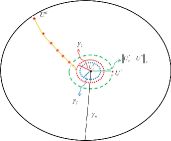
Figure 1: Convergence path of SVRG.

The comparisons on convergence results between FGD [5] and SVRG in the restricted strongly convex case are shown in Table 1. The convergence result of SVRG is presented in expectation. From Table 1, the requirement on the rank-$r$ approximation error can be relaxed from the order ${\cal O}(\frac{\sigma_{r}(X_{r}^{*})}{\kappa^{1.5}\tau(X_{r}^{*})})$ to ${\cal O}(\frac{\sigma_{r}(X_{r}^{*})}{\kappa})$, and the requirement on the radius of initialization can be relaxed from ${\cal O}(\frac{\sigma_{r}(X_{r}^{*})}{\kappa^{2}\tau^{2}(X_{r}^{*})})$ to ${\cal O}(\frac{\sigma_{r}(X_{r}^{*})}{\kappa})$, where $\kappa$ is the “condition number” of the objective function $f$ (specified in (8)), $\sigma_{r}(X_{r}^{*})$ and $\tau(X_{r}^{*})$ are respectively the $r$-th largest singular value and the condition number of the rank-$r$ approximation $X_{r}^{*}$ of the optimum $X^{*}$ with $r\leq r^{*}:=\mathrm{rank}(X^{*})$.

Algorithm	$\|X^{*}-X_{r}^{*}\|_{F}$	Initialization
FGD ([5])	${\cal O}\left(\frac{\sigma_{r}(X_{r}^{*})}{\kappa^{1.5}\tau(X_{r}^{*})}\right)$	${\cal O}\left(\frac{\sigma_{r}(X_{r}^{*})}{\kappa^{2}\tau^{2}(X_{r}^{*})}\right)$
SVRG (our)	${\color[rgb]{1,0,0}{\cal O}\left(\frac{\sigma_{r}(X_{r}^{*})}{\kappa\tau^{0.5}(X_{r}^{*})}\right)}$	${\color[rgb]{1,0,0}{\cal O}\left(\frac{\sigma_{r}(X_{r}^{*})}{\kappa\tau(X_{r}^{*})}\right)}$

Table 1: Comparisons on convergence results (in order) between FGD [5] and SVRG (this paper) in the restricted strongly convex case.

In the following, we give a corollary to show the convergence of SVRG when adopting the considered three step-size strategies (5)-(7).

Corollary 1 (Convergence for different step sizes)

Under conditions of Theorem 1, all claims in Theorem 1 hold, if one of the following conditions holds:

1. $\eta\in(0,\eta_{\max})$ when a fixed step size is adopted;

2. $m>\frac{1}{(\mu+\epsilon)\eta_{\max}}$ for any $\epsilon\geq 0$ when SBB step size is adopted.

By the definition of SBB step size (7), and Assumption 1, we have

$$\frac{1}{m(L+\epsilon)}\leq\eta_{k}\leq\frac{1}{m(\mu+\epsilon)}.$$

Thus, if $m>\frac{1}{(\mu+\epsilon)\eta_{\max}}$, then $\eta_{k}<\eta_{\max}$ for any $k\in\mathbb{N}$.

From (11)-(13), if $r=r^{*}$ then $\|X_{r}^{*}-X^{*}\|_{F}=0$, and thus $\tilde{\gamma}_{l}=0$ and $\gamma_{u}=\frac{(2+\sqrt{3})\cdot(\sqrt{2}-1)\xi\sigma_{r}(X_{r}^{*})}{3\kappa}$. However, in this case, $\gamma_{l}=\frac{(2-\sqrt{3})\cdot(\sqrt{2}-1)\xi\sigma_{r}(X_{r}^{*})}{3\kappa}>0$. Thus, we cannot claim the exact recovery of a global optimum directly from Theorem 1 even if $\|\tilde{U}^{0}-U_{r}^{*}\|^{2}_{F}\leq\gamma_{l}$. To circumvent this problem, we use a more consecutive step size, and get the following corollary showing the exact recovery of SVRG. Let

$$\bar{\eta}_{\max}:=\min\left\{\frac{L\gamma_{u}}{2B_{2}\xi},\eta_{\max}\right\}.$$ (23)

Corollary 2 (Exact recovery when $r=r^{*}$)

Let $\{\tilde{U}^{k}\}$ be a sequence generated by Algorithm 1. Let Assumptions 1 and 3 hold. If the following conditions hold: (a) $r=r^{*}$, (b) $\eta_{k}\in(0,\bar{\eta}_{\max})$, and (c) $\|\tilde{U}^{0}-U_{r}^{*}\|_{F}^{2}<\frac{(2+\sqrt{3})\cdot(\sqrt{2}-1)\xi\sigma_{r}(X_{r}^{*})}{3\kappa}$, then SVRG exactly recover the global optimum $X^{*}$ in expectation at a linear rate.

Corollary 2 shows that if fortunately, we can take $r$ as the exact rank $r^{*}$ of the global optimum, then SVRG can exactly find the global optimum in expectation exponentially fast, as long as the initialization lies in a neighborhood of the global optimum. The proof of this corollary is presented in (Supplementary Material: Section 2.2).

4 On Initialization Schemes

According to our main theorem (see, Theorem 1), the initialization should be close to $U_{r}^{*}$ to get the provable convergence. In the following, we discuss some potential initialization schemes.

Scheme I: One common way is to use one of the standard convex algorithms (say, projected gradient descent method) and obtain a good initialization $U^{0}$, then switch to SVRG to get a higher precision solution. A specific implementation of this idea has been used in [22] to deal with the matrix sensing problem, and some theoretical guarantees of this scheme have been developed in [5].

Scheme II: Another way is firstly to get $X^{0}:=\frac{1}{\|\nabla f(0)-\nabla f({\bf e}_{1}{\bf e}_{1}^{T})\|_{F}}\cdot\mathrm{Proj}_{\mathbb{S}_{+}^{p}}(-\nabla f(0))$, then take $U^{0}\in\mathbb{R}^{p\times r}$ such that $U^{0}{U^{0}}^{T}=X_{r}^{0}$, where $X_{r}^{0}$ is the rank-$r$ best approximation of $X^{0}$ via SVD, and ${\bf e}_{1}\in\mathbb{R}^{p}$ is the vector with 1 as the first component and 0 as the other components. The effectiveness of such scheme is guaranteed by [5, Corollary 12] when the objective function is well-conditioned, i.e., has a small $\kappa$.

Scheme III: Note that the previous two schemes need at least one SVD, which might be prohibitive in large scale applications. To avoid such an issue, random initialization can be exploited which actually works well in many applications.

5 Outline of Proofs

To prove Theorem 1, we need the following key lemma, which gives an error estimate of the inner loop.

Lemma 1 (A key lemma)

Let $\{U^{t}\}_{t=0}^{m}$ be the sequence at the $k$-th inner loop. Let Assumptions 1, 2 and 3 hold. Let $\eta_{k}\in(0,\eta_{\max})$. If $\gamma_{l}<\mathbb{E}[\|\tilde{U}^{k}-U_{r}^{*}\|_{F}^{2}]<\gamma_{u}$, then the sequence $\{\mathbb{E}[\|U^{t}-U_{r}^{*}\|_{F}^{2}]\}$ is monotonically decreasing for $t=0,\ldots,m$, and

$$\mathbb{E}_{i_{t}}[\|U^{t+1}-U_{r}^{*}\|_{F}^{2}]\leq\frac{\eta_{k}L}{2}\|X^{*}-X_{r}^{*}\|_{F}^{2}$$ (24)

$$+\|U^{t}-U_{r}^{*}\|_{F}^{2}-\frac{2(\sqrt{2}-1)}{3}\eta_{k}\mu\sigma_{r}(X_{r}^{*})\|U^{t}-U_{r}^{*}\|_{F}^{2}$$

$$+\frac{\eta_{k}L}{2\xi}\|U^{t}-U_{r}^{*}\|_{F}^{4}+\eta_{k}^{2}B_{2}\cdot\|\tilde{U}^{k}-U_{r}^{*}\|_{F}^{2}$$

where $B_{2}$ is specified in (17); while if $\mathbb{E}[\|\tilde{U}^{k}-U_{r}^{*}\|_{F}^{2}]\leq\gamma_{l}$, then $\mathbb{E}[\|U^{t}-U_{r}^{*}\|_{F}^{2}]\leq\gamma_{l}$ for any $t=0,\ldots,m.$

The sketch proof of Lemma 1: We prove this lemma by induction. Specifically, we first show that if $\gamma_{l}<\mathbb{E}[\|U^{t}-U_{r}^{*}\|_{F}^{2}]<\gamma_{u}$, then $\mathbb{E}[\|U^{t+1}-U_{r}^{*}\|_{F}^{2}]\leq\mathbb{E}[\|U^{t}-U_{r}^{*}\|_{F}^{2}]<\gamma_{u}$ for $t=0,\ldots,m-1$. Furthermore, $\mathbb{E}[\|U^{t+1}-U_{r}^{*}\|_{F}^{2}]$ can be estimated via noting that

$$\mathbb{E}_{i_{t}}[\|U^{t+1}-U_{r}^{*}\|_{F}^{2}]$$

$$=\|U^{t}-U_{r}^{*}\|_{F}^{2}+\eta_{k}^{2}\mathbb{E}_{i_{t}}[\|v_{k}^{t}\|_{F}^{2}]$$

$$-2\eta_{k}\mathbb{E}_{i_{t}}[\langle v_{k}^{t},U^{t}-U_{r}^{*}\rangle],$$

where $v_{k}^{t}=\nabla f_{i_{t}}(X^{t})U^{t}-\nabla f_{i_{t}}(\tilde{X}^{k})\tilde{U}^{k}+\nabla f(\tilde{X}^{k})\tilde{U}^{k}$, and then establish the bounds of both $\mathbb{E}_{i_{t}}[\|v_{k}^{t}\|_{F}^{2}]$ and $\mathbb{E}_{i_{t}}[\langle v_{k}^{t},U^{t}-U_{r}^{*}\rangle]$ via two lemmas shown in (Supplementary Material: Lemma 2 and Lemma 3), respectively. The specific proof of this lemma is presented in (Supplementary Material: Section A).

Based on Lemma 1, we show the proof of Theorem 1 as follows.

Proof of Theorem 1: By Lemma 1, if $\gamma_{l}<\|\tilde{U}^{0}-U_{r}^{*}\|_{F}^{2}<\gamma_{u}$, then for any $k\in\mathbb{N}$ and $t=0,\ldots,m-1$,

$$\mathbb{E}[\|\tilde{U}^{k+1}-U_{r}^{*}\|_{F}^{2}]\leq\mathbb{E}[\|U^{t}-U_{r}^{*}\|_{F}^{2}]\leq\mathbb{E}[\|\tilde{U}^{k}-U_{r}^{*}\|_{F}^{2}].$$

From (24) and by the definitions of $\tilde{\gamma}_{l}$ and $\tilde{\gamma}_{u}$, at the $k$-th inner loop, there holds

$$\mathbb{E}[\|U^{t+1}-U_{r}^{*}\|_{F}^{2}]-\tilde{\gamma}_{l}$$

$$\leq\left[1-\frac{\eta_{k}L}{2\xi}(\tilde{\gamma}_{u}-\mathbb{E}[\|U^{t}-U_{r}^{*}\|_{F}^{2}])\right]\times$$

$$\left(\mathbb{E}[\|U^{t}-U_{r}^{*}\|_{F}^{2}]-\tilde{\gamma}_{l}\right)+\eta_{k}^{2}B_{2}\cdot\|\tilde{U}^{k}-U_{r}^{*}\|_{F}^{2}$$

$$\leq\left[1-\frac{\eta_{k}L}{2\xi}\left(\sqrt{\tilde{\Delta}}-\sqrt{\Delta}\right)\right]\cdot(\mathbb{E}[\|U^{t}-U_{r}^{*}\|_{F}^{2}]-\tilde{\gamma}_{l})$$

$$+\eta_{k}^{2}B_{2}\cdot\|\tilde{U}^{k}-U_{r}^{*}\|_{F}^{2}$$

$$:=\rho_{k}(\mathbb{E}[\|U^{t}-U_{r}^{*}\|_{F}^{2}]-\tilde{\gamma}_{l})+\eta_{k}^{2}B_{2}\cdot\|\tilde{U}^{k}-U_{r}^{*}\|_{F}^{2},$$

where the second inequality holds for $\mathbb{E}[\|U^{t}-U_{r}^{*}\|_{F}^{2}]<\gamma_{u}$ and $\eta_{k}<\eta_{\max}\leq\frac{(\sqrt{2}-1)\mu\xi\sigma_{r}(x_{r}^{*})}{12B_{2}}\leq\frac{6}{(\sqrt{2}-1)\mu\sigma_{r}(X_{r}^{*})}\leq\frac{2\xi}{L(\sqrt{\tilde{\Delta}}-\sqrt{\Delta})}.$ By the above inequality, we have

$$\mathbb{E}[\|\tilde{U}^{k+1}-U_{r}^{*}\|_{F}^{2}]-\tilde{\gamma}_{l}=\mathbb{E}[\|U^{m}-U_{r}^{*}\|_{F}^{2}]-\tilde{\gamma}_{l}$$

$$\leq(\rho_{k})^{m}(\mathbb{E}[\|\tilde{U}^{k}-U_{r}^{*}\|_{F}^{2}]-\tilde{\gamma}_{l})$$

$$+\eta_{k}^{2}B_{2}\cdot\frac{1-(\rho_{k})^{m}}{1-\rho_{k}}\cdot\mathbb{E}[\|\tilde{U}^{k}-U_{r}^{*}\|_{F}^{2}]$$

$$\leq(\rho_{k})^{m}(\mathbb{E}[\|\tilde{U}^{k}-U_{r}^{*}\|_{F}^{2}]-\tilde{\gamma}_{l})$$

$$+\eta_{k}\theta(1-(\rho_{k})^{m})\mathbb{E}[\|\tilde{U}^{k}-U_{r}^{*}\|_{F}^{2}],$$

where the final inequality is due to the definition of $\rho_{k}$ (20), i.e., $\rho_{k}=1-\frac{\eta_{k}B_{2}}{\theta}$ and $\theta$ is specified in (18). Therefore,

$$\mathbb{E}[\|\tilde{U}^{k+1}-U_{r}^{*}\|_{F}^{2}]\leq(1-(\rho_{k})^{m})\tilde{\gamma}_{l}$$

$$+\left[(\rho_{k})^{m}+\eta_{k}\theta(1-(\rho_{k})^{m})\right]\cdot\mathbb{E}[\|\tilde{U}^{k}-U_{r}^{*}\|_{F}^{2}]$$

$$:=\tilde{\rho}_{k}\mathbb{E}[\|\tilde{U}^{k}-U_{r}^{*}\|_{F}^{2}]+(1-(\rho_{k})^{m})\tilde{\gamma}_{l}.$$

Based on the above inequality, we get (22) via a recursive way, and thus complete the proof of this theorem. $\Box$

6 Experiments

In this section, we present two application examples to show the effectiveness of the proposed algorithm and also verify our developed theoretical results.

6.1 Matrix Sensing

We consider the following matrix sensing problem

$$\mathop{\mathrm{min}}_{X\succeq 0}\quad f(X)=\frac{1}{2n}\sum_{i=1}^{n}(b_{i}-\langle A_{i},X\rangle)^{2},$$

where $X\in\mathbb{R}^{p\times p}$ is a low-rank matrix, $A_{i}\in\mathbb{R}^{p\times p}$ is a sub-Gaussian independent measurement matrix of the $i$-th sample, $b_{i}\in\mathbb{R}$, and $n\in\mathbb{N}$ is the sample size.

Specifically, we let $p=5000$, the optimal matrix $X^{*}:=U^{*}{U^{*}}^{T}$ be a low-rank matrix with $\mathrm{rank}(X^{*})=5$ and the sample size $n=10p$. In such high-dimensional regime, the generic semidefinite optimization methods generally do not work. Therefore, we only compare the performance of the low-rank factorization based methods, i.e., FGD [5], SFGD, and SVRG with three different step sizes studied in this paper. In this experiment, $r$ is set as $r^{*}$, and the initialization is constructed via the optimum $U^{*}$ with a random perturbation, and the step sizes for all algorithms are tuned in the hand-optimal way (shown in the figure). For three SVRG algorithms, the update frequency of the inner loop $m$ is set as the sample size $n$. The experiment results are shown in Figure 2. An epoch of SFGD includes $n$ iterations of SFGD, an epoch of FGD is exactly an iteration of FGD, and an epoch of SVRG is an iteration of outer loop. The iterative error curves of SVRG, SFGD and FGD are shown along epochs since all of them exploit a full scan of gradients over sample per epoch and their computational complexities per epoch are thus comparable.

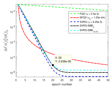
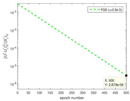
Figure 2: Experiments for matrix sensing problem. Left: trends of iterative errors of five algorithms. Right: trend of iterative error of FGD. It requires about 20, 50 and 500 epochs for SVRG, SFGD and FGD respectively, to achieve the precision $3\times 10^{-6}$.

From Figure 2, we can observe that all three SVRG algorithms converge exponentially fast to the global optimum with high precisions. To achieve the precision $3\times 10^{-6}$, it requires about 50 and 500 epochs for SFGD and FGD, respectively, while about 20 epochs are generally sufficient for three SVRG algorithms. In terms of epoch number, the considered SVRG methods are much faster than both FGD and SFGD. These experiment results demonstrate the effectiveness of SVRG and also verify our developed theoretical results.

6.2 Ordinal Embedding

In this subsection, we apply SVRG to the ordinal embedding problem, of which the Stochastic Triplet Embedding (STE) [23] is one of the typical models. The objective function is shown as follows:

$$f(X)=\frac{1}{|{\cal C}|}\sum_{c\in{\cal C}}\ell_{c}(X)+\lambda\cdot\mathrm{tr}(X),$$

where ${\cal C}$ is a set of ordinal constraints, $|{\cal C}|$ is its cardinality, and $\ell_{c}$ is the logistic loss. To show the effectiveness of the considered SVRG methods, we compare the performance of SVRG (using fixed, SBB₀ and SBB_ϵ step sizes, where $\epsilon=0.02$) with SFGD, FGD and the projected gradient descent (ProjGD) method, where the last two are batch methods.

A. Music artist dataset: We implement SVRG on the first real world dataset called Music artist dataset, collected by [11] via a web-based survey. In this dataset, there are $1032$ users and $412$ music artists. The number of triplets on the similarity between music artists is $213472$. A triplet $(i,j,k)$ indicates an ordinal constraint like $d^{2}_{ij}(X)\leq d^{2}_{ik}(X)$, which means that “music artist $i$ is more similar to artist $j$ than artist $k$”, where $d^{2}_{ij}(X)$ is the Euclidean distance between artists $i$ and $j$, $i,j,k\in\{1,\ldots,p\}$, and $p$ is the number of total kinds of music artists. Specifically, we use the data pre-processed by [23] via removing the inconsistent triplets from the original dataset. In this dataset, there are $9107$ triplets for $p=400$ artists. The genre labels for all artists are gathered using Wikipedia, to distinguish nine music genres (rock, metal, pop, dance, hip hop, jazz, country, gospel, and reggae).

For each method, we implement independently 50 trials, and then record their test errors. For each trail, $80\%$ triplets are randomly picked as the training set and the rest as the test set. All methods start with the same initial point, which is chosen randomly. Each curve in Figure 3 shows the trend of test error of one method with respect to the epoch number.

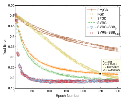
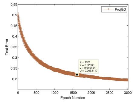
Figure 3: Experiments for Music artist data. To achieve the test error $0.22$, about 40 epochs for SVRG-SBB₀ and SVRG-SBB_0.02, and 130 epochs for SVRG (fixed step size), and 260 epochs for both SFGD and FGD, and 1600 epochs for ProjGD are required.

From Figure 3, SVRG with SBB step sizes can significantly speed up SFGD and the batch methods in terms of epoch number. Particularly, the test error curves of two SVRG-SBB methods decay much faster than those of SFGD, FGD and ProjGD at the initial 50 epochs.

B. eurodist dataset: We implement SVRG on another real world dataset called eurodist dataset, which describes the “driving” distances between 21 cities in Europe, and is available in the stats library of R. In this dataset, there are 21945 comparisons in total. A quadruplet $(i,j,k,l)$ indicates an ordinal constraint like $d^{2}_{ij}(X)\leq d^{2}_{kl}(X)$, which means that “the distance between cities $i$ and $j$ is shorter than the distance between cities $l$ and $k$”, where $d^{2}_{ij}(X)$ is the “driving” distance between cities $i$ and $j$, $i,j,k,l\in\{1,\ldots,21\}$. One of the main task of this dataset is to embed these 21 cities in 2-dimensional space.

In this experiment, we first abstract all 3990 triplet ordinal comparisons from the total data set, and then use these triplets for learning. A triplet $(i,j,k)$ indicates an ordinal constraint like $d^{2}_{ik}(X)\leq d^{2}_{jk}(X)$, which means that “the distance between cities $i$ and $k$ is less than the distance between cities $j$ and $k$”. For each method, we implement independently 50 trials, and then record their test errors. For each trail, $80\%$ triplets are randomly picked as the training set and the rest as the test set. All methods start with the same initial point, which is chosen randomly. Each curve in Figure 4 shows the trend of test error of one method with respect to the epoch number.

From Figure 4, SVRG with SBB step sizes can speed up SFGD and both batch methods in terms of epoch number. Particularly, the test error curves of two SVRG-SBB methods decay much faster than those of SFGD, FGD and ProjGD at the initial 50 epochs.

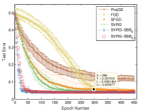
Figure 4: Experiments for eurodist dataset. To achieve the test error $0.057$, about 40 epochs for SVRG-SBB₀ and SVRG-SBB_0.1, and 150 epochs for SVRG with a fixed step size, and 300 epochs for SFGD and FGD, and more than 450 epochs for ProjGD are required.

7 Conclusion

In this paper, we consider a nonconvex stochastic semidefinite optimization problem, which emerges in many fields of science and engineering. For the first time up to our knowledge, provable global linear convergence is established for stochastic variance reduced gradient (SVRG) algorithms to solve this nonconvex problem. Specifically, under common assumptions of restricted strong convexity of the objective function and small rank-$r$ approximation error, we can show that SVRG can converge to a global optimum at a linear rate as long as the initialization lies in a neighborhood of the optimum. The initial choice condition significantly improves the existing results for deterministic gradient descent. Moreover, our choice of step sizes includes both fixed and adaptive ones using Barzilai-Borwein (BB) step size with stabilization in nonconvex settings. Application examples show that the proposed scheme is promising in fast solving some large scale problems.

Supplementary Material: Proofs

For any matrix $U\in\mathbb{R}^{p\times r}$, let $Q_{U}$ be a basis of the column space of $U$. Denote ${\cal P}_{U}:=Q_{U}Q_{U}^{T}$. Then ${\cal P}_{U}\cdot U=U$. For any matrix $Y\in\mathbb{R}^{p\times p}$, ${\cal P}_{U}Y$ is a projection of $Y$ onto the subspace spanned by $X:=UU^{T}$.

A. Proof of Lemma 1

The sketch proof of Lemma 1 is show as follows. We prove this lemma by induction. Specifically, we first show that if $\gamma_{l}<\mathbb{E}[\|U^{t}-U_{r}^{*}\|_{F}^{2}]<\gamma_{u}$, then $\mathbb{E}[\|U^{t+1}-U_{r}^{*}\|_{F}^{2}]\leq\mathbb{E}[\|U^{t}-U_{r}^{*}\|_{F}^{2}]<\gamma_{u}$ for $t=0,\ldots,m-1$. Furthermore, $\mathbb{E}[\|U^{t+1}-U_{r}^{*}\|_{F}^{2}]$ can be estimated via noting that

$$\mathbb{E}_{i_{t}}[\|U^{t+1}-U_{r}^{*}\|_{F}^{2}]$$

$$=\|U^{t}-U_{r}^{*}\|_{F}^{2}+\eta_{k}^{2}\mathbb{E}_{i_{t}}[\|v_{k}^{t}\|_{F}^{2}]$$

$$-2\eta_{k}\mathbb{E}_{i_{t}}[\langle v_{k}^{t},U^{t}-U_{r}^{*}\rangle],$$

where $v_{k}^{t}=\nabla f_{i_{t}}(X^{t})U^{t}-\nabla f_{i_{t}}(\tilde{X}^{k})\tilde{U}^{k}+\nabla f(\tilde{X}^{k})\tilde{U}^{k}$, and establishing the bounds of both $\mathbb{E}_{i_{t}}[\|v_{k}^{t}\|_{F}^{2}]$ and $\mathbb{E}_{i_{t}}[\langle v_{k}^{t},U^{t}-U_{r}^{*}\rangle]$ shown as the following two lemmas, respectively.

Lemma 2 (Bound of ${2\mathbb{E}_{i_{t}}[\langle v_{k}^{t},U^{t}-U_{r}^{*}\rangle]}$)

Let Assumptions 1 and 3 hold. Let $\{U^{t}\}_{t=0}^{m-1}$ be a sequence generated by SVRG in Algorithm 1 at the $k$-th inner loop. Let $X^{t}=U^{t}{U^{t}}^{T}$ and $v_{k}^{t}=\nabla f_{i_{t}}(X^{t})U^{t}-\nabla f_{i_{t}}(\tilde{X}^{k})\tilde{U}^{k}+\nabla f(\tilde{X}^{k})\tilde{U}^{k}$. If $\|U^{t}-U_{r}^{*}\|_{F}^{2}<\gamma_{0}\sigma_{r}(X_{r}^{*})$, then there holds

$$2\mathbb{E}_{i_{t}}[\langle v_{k}^{t},U^{t}-U_{r}^{*}\rangle]$$

$$\geq\frac{\mu}{2}\|X^{t}-X_{r}^{*}\|_{F}^{2}+\frac{\xi}{2L}\|{\cal P}_{U^{t}}\nabla f(X^{t})\|_{F}^{2}$$

$$-\frac{L}{2}\|X^{*}-X_{r}^{*}\|_{F}^{2}-\frac{L}{2\xi}\|U^{t}-U_{r}^{*}\|_{F}^{4}.$$

where $\xi$ is specified in (10).

Proof. By Assumption 3,

$$2\mathbb{E}_{i_{t}}[\langle v_{k}^{t},U^{t}-U_{r}^{*}\rangle]$$

$$=2\langle\nabla f(X^{t})U^{t},U^{t}-U_{r}^{*}\rangle$$

$$=2\langle\nabla f(X^{t}),X^{t}-U_{r}^{*}{U^{t}}^{T}\rangle$$

$$=\langle\nabla f(X^{t}),X^{t}-X_{r}^{*}\rangle$$

$$+\langle\nabla f(X^{t}),X^{t}+X_{r}^{*}-2U_{r}^{*}{U^{t}}^{T}\rangle.$$ (25)

To bound the first term of (25), we utilize the following three inequalities mainly by the Lipschitz differentiability and restricted strong convexity of $f$, that is,

(i) $$f(X_{r}^{*})\geq$$

$$f(X^{t})+\langle\nabla f(X^{t}),X_{r}^{*}-X^{t}\rangle+\frac{\mu}{2}\|X_{r}^{*}-X^{t}\|_{F}^{2},$$

(ii) $$f(X^{t})\geq f(X^{*})+(1-\bar{\eta}/2)\bar{\eta}L^{-1}\cdot\|{\cal P}_{U^{t}}\nabla f(X^{t})\|_{F}^{2},$$

(iii) $$f(X^{*})\geq f(X_{r}^{*})-\frac{L}{2}\|X^{*}-X_{r}^{*}\|_{F}^{2},$$

where (i) holds for the $(\mu,r)$-restricted strong convexity of $f$, (ii) holds the following inequality induced by the $L$-Lipschitz differentiability of $f$, i.e.,

$$f(X^{t}) \geq f(\bar{X})+\langle\nabla f(X^{t}),X^{t}-\bar{X}\rangle-\frac{L}{2}\|X^{t}-\bar{X}\|_{F}^{2}$$

$$(\text{where}\ \bar{X}:=X^{t}-\frac{\bar{\eta}}{L}{\cal P}_{U^{t}}\nabla f(X^{t}){\cal P}_{U^{t}})$$

$$=f(\bar{X})+(1-\bar{\eta}/2)\bar{\eta}L^{-1}\cdot\|{\cal P}_{U^{t}}\nabla f(X^{t})\|_{F}^{2},$$

and $f(\bar{X})\geq f(X^{*})$ since $X^{*}$ is an optimum and $\bar{X}$ is a feasible point by Lemma 8(b), and (iii) holds for the $L$-Lipschitz differentiability of $f$ and the optimality condition $\nabla f(X^{*})U^{*}=0$, i.e.,

$$f(X_{r}^{*}) \leq f(X^{*})+\langle\nabla f(X^{*}),X^{*}-X_{r}^{*}\rangle+\frac{L}{2}\|X^{*}-X_{r}^{*}\|_{F}^{2}$$

$$=f(X^{*})+\frac{L}{2}\|X^{*}-X_{r}^{*}\|_{F}^{2},$$

where the equality holds for $\nabla f(X^{*})U^{*}=0$, which directly implies the following facts: $\nabla f(X^{*})U_{r}^{*}=0$, $\nabla f(X^{*})X^{*}=0$ and $\nabla f(X^{*})X_{r}^{*}=0$ due to $X^{*}=U^{*}{U^{*}}^{T}$ and $X_{r}^{*}=U_{r}^{*}{U_{r}^{*}}^{T}$. Summing the inequalities (i)-(iii) yields

$$\langle\nabla f(X^{t}),X^{t}-X_{r}^{*}\rangle\geq\frac{\mu}{2}\|X^{t}-X_{r}^{*}\|_{F}^{2}$$ (26)

$$+(1-\bar{\eta}/2)\bar{\eta}L^{-1}\cdot\|{\cal P}_{U^{t}}\nabla f(X^{t})\|_{F}^{2}-\frac{L}{2}\|X^{*}-X_{r}^{*}\|_{F}^{2}.$$

On the other hand, we observe that

$$\langle\nabla f(X^{t}),X^{t}+X_{r}^{*}-2U_{r}^{*}{U^{t}}^{T}\rangle$$

$$=\langle{\cal P}_{U^{t}}\nabla f(X^{t})+({\bf I}-{\cal P}_{U^{t}})\nabla f(X^{t}),X^{t}+X_{r}^{*}-2U_{r}^{*}{U^{t}}^{T}\rangle$$

$$=\langle{\cal P}_{U^{t}}\nabla f(X^{t}),X^{t}+X_{r}^{*}-2U_{r}^{*}{U^{t}}^{T}\rangle$$

$$=\langle{\cal P}_{U^{t}}\nabla f(X^{t}),(U^{t}-U_{r}^{*})(U-U_{r}^{*})^{T}\rangle$$

$$\geq-\frac{(1-\bar{\eta}/2)\bar{\eta}}{2L}\|{\cal P}_{U^{t}}\nabla f(X^{t})\|_{F}^{2}$$

$$-\frac{L}{2\bar{\eta}(1-\bar{\eta}/2)}\cdot\|U^{t}-U_{r}^{*}\|_{F}^{4}.$$ (27)

where the second equality is due to $\langle({\bf I}-{\cal P}_{U^{t}})\nabla f(X^{t}),X^{t}\rangle=0$, $\langle({\bf I}-{\cal P}_{U^{t}})\nabla f(X^{t}),U_{r}^{*}{U^{t}}^{T}\rangle=0$ and $\langle({\bf I}-{\cal P}_{U^{t}})\nabla f(X^{t}),X_{r}^{*}\rangle=0$ by Lemma 8(c), the last equality holds for $X_{r}^{*}=U_{r}^{*}{U_{r}^{*}}^{T}$, and the inequality holds for the basic inequality: $\langle Y,Z\rangle\geq-\frac{c}{2}\|Y\|_{F}^{2}-\frac{1}{2c}\|Z\|_{F}^{2}$ for any $Y,Z\in\mathbb{R}^{p\times p}$ and $c>0$. Substituting (26) and (27) into (25) concludes this lemma. $\Box$

Lemma 3 (Bound of ${\mathbb{E}_{i_{t}}[\|v_{k}^{t}\|_{F}^{2}]}$)

Let Assumptions 1, 2 and 3 hold. Assume that $\|U^{t}-U_{r}^{*}\|^{2}_{F}<\gamma_{u}$ and $\|\tilde{U}^{k}-U_{r}^{*}\|^{2}_{F}<\gamma_{u}$, then

$$\mathbb{E}_{i_{t}}[\|v_{k}^{t}\|_{F}^{2}] \leq 4(B_{0}+B_{1})(\|U^{t}-U_{r}^{*}\|_{F}^{2}+\|\tilde{U}^{k}-U_{r}^{*}\|_{F}^{2})$$

$$+4L^{2}{\cal B}(\|X^{t}-X_{r}^{*}\|_{F}^{2}+\|\tilde{X}^{k}-X_{r}^{*}\|_{F}^{2})$$

$$+\|{\cal P}_{U^{t}}\nabla f(X^{t})\|_{F}^{2}\cdot\|X^{t}\|_{F}.$$

Proof. Note that

$$\|v_{k}^{t}\|_{F}^{2} =\|\nabla f_{i_{t}}(X^{t})U^{t}-\nabla f_{i_{t}}(\tilde{X}^{k})\tilde{U}^{k}\|_{F}^{2}$$

$$+\|\nabla f(\tilde{X}^{k})\tilde{U}^{k}\|_{F}^{2}$$

$$+2\langle\nabla f_{i_{t}}(X^{t})U^{t}-\nabla f_{i_{t}}(\tilde{X}^{k})\tilde{U}^{k},\nabla f(\tilde{X}^{k})\tilde{U}^{k}\rangle.$$

Thus,

$$\mathbb{E}_{i_{t}}[\|v_{k}^{t}\|_{F}^{2}]$$

$$=\mathbb{E}_{i_{t}}[\|\nabla f_{i_{t}}(X^{t})U^{t}-\nabla f_{i_{t}}(\tilde{X}^{k})\tilde{U}^{k}\|_{F}^{2}]$$

$$+\|\nabla f(\tilde{X}^{k})\tilde{U}^{k}\|_{F}^{2}$$

$$+2\langle\nabla f(X^{t})U^{t}-\nabla f(\tilde{X}^{k})\tilde{U}^{k},\nabla f(\tilde{X}^{k})\tilde{U}^{k}\rangle$$

$$=\mathbb{E}_{i_{t}}[\|\nabla f_{i_{t}}(X^{t})U^{t}-\nabla f_{i_{t}}(\tilde{X}^{k})\tilde{U}^{k}\|_{F}^{2}]$$

$$-\|\nabla f(X^{t})U^{t}-\nabla f(\tilde{X}^{k})\tilde{U}^{k}\|_{F}^{2}+\|\nabla f(X^{t})U^{t}\|_{F}^{2}$$

$$\leq\mathbb{E}_{i_{t}}[\|\nabla f_{i_{t}}(X^{t})U^{t}-\nabla f_{i_{t}}(\tilde{X}^{k})\tilde{U}^{k}\|_{F}^{2}]$$

$$+\|{\cal P}_{U^{t}}\nabla f(X^{t})\|_{F}^{2}\cdot\|X^{t}\|_{F},$$ (28)

where the last inequality holds for $\|\nabla f(X^{t})U^{t}-\nabla f(\tilde{X}^{k})\tilde{U}^{k}\|_{F}^{2}\geq 0$ and

$$\|\nabla f(X^{t})U^{t}\|_{F}^{2}$$

$$=\|{\cal P}_{U^{t}}\nabla f(X^{t})U^{t}+({\bf I}-{\cal P}_{U^{t}})\nabla f(X^{t})U^{t}\|_{F}^{2}$$

$$=\|{\cal P}_{U^{t}}\nabla f(X^{t})U^{t}\|^{2}$$

$$\leq\|{\cal P}_{U^{t}}\nabla f(X^{t})\|_{F}^{2}\cdot\|X^{t}\|_{F}.$$

In the following, we bound the first term of (A. Proof of Lemma 1). Note that

$$\|\nabla f_{i_{t}}(X^{t})U^{t}-\nabla f_{i_{t}}(\tilde{X}^{k})\tilde{U}^{k}\|_{F}^{2}$$

$$=\|\nabla f_{i_{t}}(X^{t})(U^{t}-\tilde{U}^{k})+(\nabla f_{i_{t}}(X^{t})-\nabla f_{i_{t}}(\tilde{X}^{k}))\tilde{U}^{k}\|_{F}^{2}$$

$$\leq 2\|\nabla f_{i_{t}}(X^{t})(U^{t}-\tilde{U}^{k})\|_{F}^{2}$$

$$+2\|(\nabla f_{i_{t}}(X^{t})-\nabla f_{i_{t}}(\tilde{X}^{k}))\tilde{U}^{k}\|_{F}^{2}$$

$$\leq 2\|\nabla f_{i_{t}}(X^{t})\|_{F}^{2}\|U^{t}-\tilde{U}^{k}\|_{F}^{2}$$

$$+2L^{2}\|\tilde{X}^{k}\|_{F}\|X^{t}-\tilde{X}^{k}\|_{F}^{2},$$

which follows

$$\mathbb{E}_{i_{t}}[\|\nabla f_{i_{t}}(X^{t})U^{t}-\nabla f_{i_{t}}(\tilde{X}^{k})\tilde{U}^{k}\|_{F}^{2}]$$

$$\leq 2(\mathbb{E}_{i_{t}}[\|\nabla f_{i_{t}}(X^{t})\|_{F}^{2}]-\|\nabla f(X^{t})\|_{F}^{2})\|U^{t}-\tilde{U}^{k}\|_{F}^{2}$$

$$+2\|\nabla f(X^{t})\|_{F}^{2}\cdot\|U^{t}-\tilde{U}^{k}\|_{F}^{2}+2L^{2}\|\tilde{X}^{k}\|_{F}\|X^{t}-\tilde{X}^{k}\|_{F}^{2}$$

$$\leq 2(B_{0}+B_{1})\cdot\|U^{t}-\tilde{U}^{k}\|_{F}^{2}+2L^{2}{\cal B}\|X^{t}-\tilde{X}^{k}\|_{F}^{2}$$

$$\leq 4(B_{0}+B_{1})\cdot(\|U^{t}-U_{r}^{*}\|_{F}^{2}+\|\tilde{U}^{k}-U_{r}^{*}\|_{F}^{2})$$

$$+4L^{2}{\cal B}(\|X^{t}-X_{r}^{*}\|_{F}^{2}+\|\tilde{X}^{k}-X_{r}^{*}\|_{F}^{2}),$$

where $B_{0}$, $B_{1}$ and ${\cal B}$ are specified before (17). Substituting the above inequality into (A. Proof of Lemma 1), we can conclude this lemma. $\Box$

Based on the above two lemmas, we give the proof of Lemma 1.

Proof of Lemma 1: By Lemma 2 and Lemma 3,

$$\mathbb{E}_{i_{t}}[\|U^{t+1}-U_{r}^{*}\|_{F}^{2}]\leq\|U^{t}-U_{r}^{*}\|_{F}^{2}$$

$$-\eta_{k}\left[\frac{\mu}{2}\|X^{t}-X_{r}^{*}\|_{F}^{2}+\frac{\xi}{2L}\|{\cal P}_{U^{t}}\nabla f(X^{t})\|_{F}^{2}\right]$$

$$+\eta_{k}\left[\frac{L}{2}\|X^{*}-X_{r}^{*}\|_{F}^{2}+\frac{L}{2\xi}\|U^{t}-U_{r}^{*}\|_{F}^{4}\right]$$

$$+4\eta_{k}^{2}(B_{0}+B_{1})(\|U^{t}-U_{r}^{*}\|_{F}^{2}+\|\tilde{U}^{k}-U_{r}^{*}\|_{F}^{2})$$

$$+4\eta_{k}^{2}L^{2}{\cal B}\left(\|X^{t}-X_{r}^{*}\|_{F}^{2}+\|\tilde{X}^{k}-X_{r}^{*}\|_{F}^{2}\right)$$

$$+\eta_{k}^{2}\|{\cal P}_{U^{t}}\nabla f(X^{t})\|_{F}^{2}\cdot\|X^{t}\|_{F}$$

$$\leq\|U^{t}-U_{r}^{*}\|_{F}^{2}-\left(\frac{\eta_{k}\mu}{2}-4\eta_{k}^{2}L^{2}{\cal B}\right)\|X^{t}-X_{r}^{*}\|_{F}^{2}$$

$$+4\eta_{k}^{2}(B_{0}+B_{1})\|U^{t}-U_{r}^{*}\|_{F}^{2}+\frac{\eta_{k}L}{2\xi}\|U^{t}-U_{r}^{*}\|_{F}^{4}$$

$$+4\eta_{k}^{2}\left[L^{2}{\cal B}\|\tilde{X}^{k}-X_{r}^{*}\|_{F}^{2}+(B_{0}+B_{1})\|\tilde{U}^{k}-U_{r}^{*}\|_{F}^{2}\right]$$

$$+\frac{\eta_{k}L}{2}\|X^{*}-X_{r}^{*}\|_{F}^{2}$$

$$\leq\|U^{t}-U_{r}^{*}\|_{F}^{2}-\eta_{k}\|U^{t}-U_{r}^{*}\|_{F}^{2}\times$$

$$\left[2(\sqrt{2}-1)\sigma_{r}(X_{r}^{*})\left(\frac{\mu}{2}-4\eta_{k}L^{2}{\cal B}\right)-4\eta_{k}(B_{0}+B_{1})\right]$$

$$+\frac{\eta_{k}L}{2\xi}\|U^{t}-U_{r}^{*}\|_{F}^{4}$$

$$+4\eta_{k}^{2}\left[L^{2}{\cal B}\|\tilde{X}^{k}-X_{r}^{*}\|_{F}^{2}+(B_{0}+B_{1})\|\tilde{U}^{k}-U_{r}^{*}\|_{F}^{2}\right]$$

$$+\frac{\eta_{k}L}{2}\|X^{*}-X_{r}^{*}\|_{F}^{2},$$

$$\leq\|U^{t}-U_{r}^{*}\|_{F}^{2}+\frac{\eta_{k}L}{2\xi}\|U^{t}-U_{r}^{*}\|_{F}^{4}-\eta_{k}\|U^{t}-U_{r}^{*}\|_{F}^{2}\times$$

$$\left[2(\sqrt{2}-1)\sigma_{r}(X_{r}^{*})\left(\frac{\mu}{2}-4\eta_{k}L^{2}{\cal B}\right)-4\eta_{k}(B_{0}+B_{1})\right]$$

$$+4\eta_{k}^{2}\left[2L^{2}{\cal B}({\cal B}+\|X_{r}^{*}\|_{F})+B_{0}+B_{1}\right]\cdot\|\tilde{U}^{k}-U_{r}^{*}\|_{F}^{2}$$

$$+\frac{\eta_{k}L}{2}\|X^{*}-X_{r}^{*}\|_{F}^{2},$$

where the first inequality is due to Lemma 2 and Lemma 3, the second inequality holds for $\eta_{k}<\eta_{\max}\leq\frac{\xi}{2{\cal B}L}$, the third inequality holds for $\eta_{k}<\eta_{\max}\leq\frac{1}{8{\cal B}\kappa L}$ and Lemma 5(b), the final inequality holds for Lemma 5(a). Since $\eta_{k}<\eta_{\max}\leq\frac{(\sqrt{2}-1)\mu\sigma_{r}(X_{r}^{*})}{12[2(\sqrt{2}-1)\sigma_{r}(X_{r}^{*})L^{2}{\cal B}+B_{0}+B_{1}]}$, then

$$2(\sqrt{2}-1)\sigma_{r}(X_{r}^{*})\left(\frac{\mu}{2}-4\eta_{k}L^{2}{\cal B}\right)-4\eta_{k}(B_{0}+B_{1})$$

$$\geq\frac{2(\sqrt{2}-1)\mu\sigma_{r}(X_{r}^{*})}{3}.$$

Thus, substituting the above inequality into the first main inequality yields (24).

Furthermore, by the assumption of this lemma and $\gamma_{u}\leq\gamma_{0}\sigma_{r}(X_{r}^{*})$, we have

$$\|\tilde{U}^{k}-U_{r}^{*}\|_{F}^{2}<\gamma_{0}\sigma_{r}(X_{r}^{*}).$$

Thus,

$$\mathbb{E}_{i_{t}}[\|U^{t+1}-U_{r}^{*}\|_{F}^{2}]$$

$$\leq\|U^{t}-U_{r}^{*}\|_{F}^{2}+\frac{\eta_{k}L}{2\xi}\times$$

$$\left[\|U^{t}-U_{r}^{*}\|_{F}^{4}+\xi\|X^{*}-X_{r}^{*}\|_{F}^{2}+\frac{2\xi\eta_{k}B_{2}}{L}\cdot\gamma_{0}\sigma_{r}(X_{r}^{*})\right]$$

$$-\frac{\eta_{k}L}{2\xi}\cdot\frac{4(\sqrt{2}-1)\xi\sigma_{r}(X_{r}^{*})}{3\kappa}\|U^{t}-U_{r}^{*}\|_{F}^{2}$$ (29)

$$\leq\|U^{t}-U_{r}^{*}\|_{F}^{2}+\frac{\eta_{k}L}{2\xi}\times$$

$$\left[\|U^{t}-U_{r}^{*}\|_{F}^{4}-\frac{4(\sqrt{2}-1)\xi\sigma_{r}(X_{r}^{*})}{3\kappa}\|U^{t}-U_{r}^{*}\|_{F}^{2}\right]$$

$$+\frac{\eta_{k}L}{2\xi}\cdot\left[\xi\|X^{*}-X_{r}^{*}\|_{F}^{2}+\frac{(\sqrt{2}-1)^{2}\xi^{2}\sigma_{r}^{2}(X_{r}^{*})}{9\kappa^{2}}\right],$$

where the second inequality holds for $\eta_{k}<\eta_{\max}\leq\frac{(\sqrt{2}-1)\mu\xi\sigma_{r}(X_{r}^{*})}{12B_{2}}$, and $\eta_{k}<\eta_{\max}\leq\frac{(\sqrt{2}-1)^{2}\xi\mu\sigma_{r}(X_{r}^{*})}{18\kappa B_{2}\gamma_{0}}$. By the definitions of $\gamma_{l}$ (11) and $\gamma_{u}$ (12), the above inequality implies

$$\mathbb{E}_{i_{t}}[\|U^{t+1}-U_{r}^{*}\|_{F}^{2}]\leq\|U^{t}-U_{r}^{*}\|_{F}^{2}$$

$$-\frac{\eta_{k}L}{2\xi}(\gamma_{u}-\|U^{t}-U_{r}^{*}\|_{F}^{2})(\|U^{t}-U_{r}^{*}\|_{F}^{2}-\gamma_{l}),$$

which implies $\mathbb{E}[\|U^{t+1}-U_{r}^{*}\|_{F}^{2}]\leq\mathbb{E}[\|U^{t}-U_{r}^{*}\|_{F}^{2}]$ if $\gamma_{l}<\mathbb{E}[\|U^{t}-U_{r}^{*}\|_{F}^{2}]<\gamma_{u}$. Inductively, we can claim the first part of this lemma.

Define a univariate function $h(z)=z-\frac{\eta_{k}L}{2\xi}\cdot\left((\gamma_{l}+\gamma_{u})z-z^{2}-\gamma_{l}\cdot\gamma_{u}\right)$ for any $z\in\mathbb{R}_{+}$. Then its derivative is

$$h^{\prime}(z)=1-\frac{\eta_{k}L}{2\xi}\cdot(\gamma_{l}+\gamma_{u})+\frac{\eta_{k}L}{\xi}\cdot z$$

$$=1-(\sqrt{2}-1)\eta_{k}\mu\sigma_{r}(X_{r}^{*})+\frac{\eta_{k}L}{\xi}\cdot z>0,$$

for $0<z\leq\gamma_{l}$, where the second equality holds for (15), and the inequality is due to $1-(\sqrt{2}-1)\eta_{k}\mu\sigma_{r}(X_{r}^{*})>0$ for any $\eta_{k}\in(0,\eta_{\max})$. Thus, for any $0<z\leq\gamma_{l}$,

$$h(z)\leq h(\gamma_{l})=\gamma_{l},$$

which shows that the last statement of this lemma holds. Therefore, we end the proof of this lemma. $\Box$

B. Proof of Corollary 2

Proof. Note that $\bar{\eta}_{\max}\leq\eta_{\max}$. By Theorem 1, if

$$\gamma_{l}:=\frac{(2-\sqrt{3})\cdot(\sqrt{2}-1)\xi\sigma_{r}(X_{r}^{*})}{3\kappa}$$

$$<\|\tilde{U}^{0}-U_{r}^{*}\|_{F}^{2}<\frac{(2+\sqrt{3})\cdot(\sqrt{2}-1)\xi\sigma_{r}(X_{r}^{*})}{3\kappa}:=\gamma_{u},$$

then it is obvious that SVRG converges to the optimum $X^{*}$ at a linear rate. As a consequence, we only need to prove the exact recovery of SVRG when $\|\tilde{U}^{0}-U_{r}^{*}\|_{F}^{2}\leq\gamma_{l}$. By Theorem 1, in this case, $\mathbb{E}[\|\tilde{U}^{k}-U_{r}^{*}\|_{F}^{2}]\leq\gamma_{l}$ for all $k\in\mathbb{N}$. Actually, by the proof of Theorem 1, at any $k$-th inner loop,

$$\mathbb{E}[\|\tilde{U}^{t}-U_{r}^{*}\|_{F}^{2}]\leq\gamma_{l}$$ (30)

for any $t=1,\ldots,m$.

In this case, it is obvious that Lemmas 2 and 3 still hold, and (29) in the proof of Lemma 1 should be revised as

$$\mathbb{E}_{i_{t}}[\|U^{t+1}-U_{r}^{*}\|_{F}^{2}]$$

$$\leq\|U^{t}-U^{*}\|_{F}^{2}+\frac{\eta_{k}L}{2\xi}\times$$

$$\left[\|U^{t}-U^{*}\|_{F}^{4}-\frac{4(\sqrt{2}-1)\xi\sigma_{r}(X_{r}^{*})}{3\kappa}\|U^{t}-U^{*}\|_{F}^{2}\right]$$

$$+\eta_{k}^{2}B_{2}\cdot\|\tilde{U}^{k}-U^{*}\|_{F}^{2}$$

$$\leq\left(1-\frac{\eta_{k}L}{2\xi}\cdot\gamma_{u}\right)\cdot\|U^{t}-U^{*}\|_{F}^{2}$$

$$+\eta_{k}^{2}B_{2}\cdot\|\tilde{U}^{k}-U^{*}\|_{F}^{2},$$ (31)

where the second inequality holds for (30) and (15). By (31), recursively, after some simplifications we have

$$\mathbb{E}[\|\tilde{U}^{k+1}-U^{*}\|_{F}^{2}]$$ (32)

$$\leq\left(1-\frac{\eta_{k}L}{2\xi}\cdot\gamma_{u}\right)^{m}\|\tilde{U}^{k}-U^{*}\|_{F}^{2}$$

$$+\frac{2B_{2}\eta_{k}\xi}{L\gamma_{u}}\cdot\left[1-\left(1-\frac{\eta_{k}L}{2\xi}\cdot\gamma_{u}\right)^{m}\right]\|\tilde{U}^{k}-U^{*}\|_{F}^{2}$$

Since $\eta_{k}\in(0,\bar{\eta}_{\max})$, then

$$0<\frac{2B_{2}\eta_{k}\xi}{L\gamma_{u}}<1,$$

and thus,

$$0<\left(1-\frac{\eta_{k}L}{2\xi}\cdot\gamma_{u}\right)^{m}$$

$$+\frac{2B_{2}\eta_{k}\xi}{L\gamma_{u}}\cdot\left[1-\left(1-\frac{\eta_{k}L}{2\xi}\cdot\gamma_{u}\right)^{m}\right]<1,$$

which implies that SVRG converges to $X^{*}$ at a linear rate. Therefore, we finish the proof of this corollary. $\Box$

C. Several Useful Lemmas

Lemma 4 ([1])

Let $A$ and $B$ be two positive semi-definite matrices with the size $p\times p$. Assume that $A$ is full rank, then

$$\mathrm{tr}(AB)\geq\sigma_{\min}(A)\mathrm{tr}(B).$$

Lemma 5

For any $U\in\mathbb{R}^{p\times r},$ let $X=UU^{T}$, $X_{r}^{*}=U_{r}^{*}{U_{r}^{*}}^{T}$, the following hold:

1. (Upper bound) $\|X-X_{r}^{*}\|_{F}^{2}\leq 2(\|X\|_{F}+\|X_{r}^{*}\|_{F})\cdot\|U-U_{r}^{*}\|_{F}^{2}$, and

2. (Lower bound) if $\|U-U_{r}^{*}\|_{F}\leq\gamma\sigma_{r}(U_{r}^{*})$ for some $0<\gamma<1$, then

   $$\|X-X_{r}^{*}\|_{F}^{2}\geq 2(\sqrt{2}-1)\sigma_{r}^{2}(U_{r}^{*})\|U-U_{r}^{*}\|_{F}^{2}.$$

Proof. (a) Note that

$$\|UU^{T}-U_{r}^{*}{U_{r}^{*}}^{T}\|_{F} =\|U(U-U_{r}^{*})^{T}+(U-U_{r}^{*}){U_{r}^{*}}^{T}\|_{F}$$

$$\leq(\|U\|_{F}+\|U_{r}^{*}\|_{F})\|U-U_{r}^{*}\|_{F}.$$

Thus, $\|X-X_{r}^{*}\|_{F}^{2}\leq(\|U\|_{F}+\|U_{r}^{*}\|_{F})^{2}\|U-U_{r}^{*}\|_{F}^{2}\leq 2(\|U\|_{F}^{2}+\|U_{r}^{*}\|_{F}^{2})\|U-U_{r}^{*}\|_{F}^{2}.$

(b) For any $x\in\mathbb{R}^{r}$, note that

$$2x^{T}U^{T}U_{r}^{*}x =\|Ux\|_{2}^{2}+\|U_{r}^{*}x\|_{2}^{2}-\|(U-U_{r}^{*})x\|_{2}^{2}$$

$$\geq\|U_{r}^{*}x\|_{2}^{2}-\|U-U_{r}^{*}\|_{2}^{2}\cdot\|x\|_{2}^{2}$$

$$\geq(1-\gamma^{2})\sigma_{r}{(X_{r}^{*})}\|x\|_{2}^{2}$$

$$\geq 0\quad(\because 0<\gamma<1),$$ (33)

where the first inequality is due to $\|Ux\|_{2}^{2}\geq 0$ and $\|(U-U_{r}^{*})x\|_{2}\leq\|U-U_{r}^{*}\|_{2}\cdot\|x\|_{2}$, and the second inequality holds for $\|U_{r}^{*}x\|_{2}^{2}\geq\sigma_{r}(X_{r}^{*})\|x\|_{2}^{2}$ and $\|U-U_{r}^{*}\|_{2}^{2}\leq\|U-U_{r}^{*}\|_{F}^{2}\leq\gamma^{2}\sigma_{r}(X_{r}^{*})$ by the assumption of this lemma. Thus, (C. Several Useful Lemmas) implies

$$U^{T}U_{r}^{*}\succ 0,$$ (34)

and $U^{T}U_{r}^{*}$ is full rank. Based on (34), we prove part (b). Let $H=U-U_{r}^{*}$. Then

$$\|X-X_{r}^{*}\|_{F}^{2} =\mathrm{tr}\left((H^{T}H)^{2}+4H^{T}HH^{T}U_{r}^{*}\right)$$

$$+\mathrm{tr}\left(2(H^{T}U_{r}^{*})^{2}+2{U_{r}^{*}}^{T}{U_{r}^{*}}H^{T}H\right).$$

Thus, establishing Lemma 5(b) is equivalent to show that

$$\mathrm{tr}\left((H^{T}H)^{2}+4H^{T}HH^{T}{U_{r}^{*}}+2(H^{T}{U_{r}^{*}})^{2}\right)$$

$$+\mathrm{tr}\left(2{U_{r}^{*}}^{T}{U_{r}^{*}}H^{T}H-cH^{T}H\right)$$

$$\geq 0,$$

where $c:=2(\sqrt{2}-1)\sigma_{r}^{2}({U_{r}^{*}})$. By some simple derivations, we can observe that

$$\mathrm{tr}\left((H^{T}H)^{2}+4H^{T}HH^{T}{U_{r}^{*}}+2(H^{T}{U_{r}^{*}})^{2}\right)$$

$$+\mathrm{tr}\left(2{U_{r}^{*}}^{T}{U_{r}^{*}}H^{T}H-cH^{T}H\right)$$

$$=\mathrm{tr}\left((H^{T}H+\sqrt{2}H^{T}{U_{r}^{*}})^{2}+(4-2\sqrt{2})H^{T}HH^{T}{U_{r}^{*}}\right)$$

$$+\mathrm{tr}\left(2{U_{r}^{*}}^{T}{U_{r}^{*}}H^{T}H-cH^{T}H\right)$$

$$\geq\mathrm{tr}\left((4-2\sqrt{2})H^{T}HH^{T}{U_{r}^{*}}+2{U_{r}^{*}}^{T}{U_{r}^{*}}H^{T}H-cH^{T}H\right)$$

$$=\mathrm{tr}\left(\left((4-2\sqrt{2})H^{T}{U_{r}^{*}}+2{U_{r}^{*}}^{T}{U_{r}^{*}}-c{\bf I}\right)\cdot H^{T}H\right).$$

Recalling $H^{T}{U_{r}^{*}}=U^{T}{U_{r}^{*}}-{U_{r}^{*}}^{T}{U_{r}^{*}}$, we have

$$\mathrm{tr}\left(\left((4-2\sqrt{2})H^{T}{U_{r}^{*}}+2{U_{r}^{*}}^{T}{U_{r}^{*}}-c{\bf I}\right)\cdot H^{T}H\right)$$

$$=\mathrm{tr}\left((4-2\sqrt{2})U^{T}{U_{r}^{*}}\cdot H^{T}H\right)$$

$$+\mathrm{tr}\left(\left(2(\sqrt{2}-1){U_{r}^{*}}^{T}{U_{r}^{*}}-c{\bf I}\right)\cdot H^{T}H\right)$$

$$=\mathrm{tr}\left((2-\sqrt{2})(U^{T}{U_{r}^{*}}+{U_{r}^{*}}^{T}U)\cdot H^{T}H\right)$$

$$+\mathrm{tr}\left(\left(2(\sqrt{2}-1){U_{r}^{*}}^{T}{U_{r}^{*}}-c{\bf I}\right)\cdot H^{T}H\right)$$

$$\geq\mathrm{tr}\left(\left(2(\sqrt{2}-1){U_{r}^{*}}^{T}{U_{r}^{*}}-c{\bf I}\right)\cdot H^{T}H\right)$$

$$\geq 0,\quad(\because c:=2(\sqrt{2}-1)\sigma_{r}^{2}({U_{r}^{*}}),\ \text{Lemma}\ \ref{Lemm:trace})$$

where the second equality is due to $\mathrm{tr}(U^{T}{U_{r}^{*}}H^{T}H)=\mathrm{tr}(H^{T}H{U_{r}^{*}}^{T}U)=\mathrm{tr}({U_{r}^{*}}^{T}UH^{T}H)$, and the first inequality holds for (34) and Lemma 4. Therefore, the above inequality implies

$$\mathrm{tr}\left((H^{T}H)^{2}+4H^{T}HH^{T}{U_{r}^{*}}+2(H^{T}{U_{r}^{*}})^{2}\right)$$

$$+\mathrm{tr}\left(2{U_{r}^{*}}^{T}{U_{r}^{*}}H^{T}H-cH^{T}H\right)\geq 0,$$

which concludes part (b) of this lemma. $\Box$

The following lemma is similar to [5, Lemma 18].

Lemma 6

Let $X=UU^{T}$ and $X_{r}^{*}=U_{r}^{*}{U_{r}^{*}}^{T}$ be two $p\times p$ rank-$r$ positive semidefinite matrices. Let $\|U-U_{r}^{*}\|_{F}\leq\gamma\sigma_{r}(U_{r}^{*})$ for some constant $0<\gamma<1$. Then

$$\|X-X_{r}^{*}\|_{F}\leq(2\gamma+\gamma^{2})\cdot\tau(U_{r}^{*})\cdot\sigma_{r}(X_{r}^{*}),$$

where $\tau(U_{r}^{*}):=\frac{\sigma_{1}(U_{r}^{*})}{\sigma_{r}(U_{r}^{*})}$.

Proof. Note that

$$\|X-X_{r}^{*}\|_{F} =\|U(U-{U_{r}^{*}})^{T}+(U-U_{r}^{*}){U_{r}^{*}}^{T}\|_{F}$$

$$\leq\|U-U_{r}^{*}\|_{F}(\|U\|_{2}+\|U_{r}^{*}\|_{2})$$

$$\leq(2\|U_{r}^{*}\|_{2}+\gamma\sigma_{r}(U_{r}^{*}))\|U-U_{r}^{*}\|_{F}$$

$$\leq(2+\gamma)\gamma\cdot\|U_{r}^{*}\|_{2}\cdot\sigma_{r}(U_{r}^{*}),$$

where the first inequality holds for the triangle inequality, Cauchy-Schwartz inequality and the fact that the spectral norm is invariant with respect to the orthogonal transformation, the second inequality is due to the following sequence of inequalities, based on the hypothesis of the lemma:

$$\|U\|_{2}-\|U_{r}^{*}\|_{2}\leq\|U-U_{r}^{*}\|_{2}\leq\|U-U_{r}^{*}\|_{F}\leq\gamma\sigma_{r}(U_{r}^{*}),$$

and the last inequality holds for the fact $\sigma_{r}(U_{r}^{*})\leq\|U_{r}^{*}\|_{2}$ and the assumption of this lemma. The above inequality directly implies the claim of this lemma by the definition of $\tau(U_{r}^{*})$. $\Box$

Moreover, we need modify [5, Lemma 19] as follows.

Lemma 7

Let $X=UU^{T}$ and $X_{r}^{*}=U_{r}^{*}{U_{r}^{*}}^{T}$ be two $p\times p$ rank-$r$ positive semidefinite matrices. Let $\|U-U_{r}^{*}\|_{F}\leq\gamma\sigma_{r}(U_{r}^{*})$ for some constant $0<\gamma<1$. Then

$$\sigma_{r}(U)\geq(1-\gamma)\sigma_{r}(U_{r}^{*}).$$

Proof. Using the norm ordering $\|\cdot\|_{2}\leq\|\cdot\|_{F}$ and the Weyl’s inequality for perturbation of singular values (see, [2, Theorem 3.3.16]), we get

$$|\sigma_{i}(U)-\sigma_{i}(U_{r}^{*})|\leq\gamma\sigma_{r}(U_{r}^{*}),\ 1\leq i\leq r,$$

which implies that

$$\sigma_{r}(U)\geq(1-\gamma)\sigma_{r}(U_{r}^{*}).$$

$\Box$

Lemma 8

Let Assumption 1 hold. Let $X=UU^{T}$ and $X_{r}^{*}=U_{r}^{*}{U_{r}^{*}}^{T}$ be two $p\times p$ rank-$r$ ($r<p$) positive semidefinite matrices. Suppse that $\|U-U_{r}^{*}\|^{2}_{F}<\gamma_{0}\sigma_{r}(X_{r}^{*})$, where $\gamma_{0}$ is specified in (8). Then the following hold:

1. (Bounded gradient)

   $$\|\nabla f(X)\|_{F}$$

   $$\leq\|\nabla f(X_{r}^{*})\|_{F}+(2\sqrt{\gamma_{0}}+\gamma_{0})L\tau(U_{r}^{*})\sigma_{r}(X_{r}^{*}),$$

2. (Feasibility of $\bar{X}$) Let $\bar{X}:=X-\frac{\bar{\eta}}{L}{\cal P}_{U}\nabla f(X){\cal P}_{U}$, where $\bar{\eta}$ is specified in (9), then $\bar{X}$ is a feasible point, i.e., $\bar{X}$ is symmetric and positive semidefinite.

3. $({\bf I}-{\cal P}_{U})X_{r}^{*}=0.$

Proof. (a) Note that

$$\|\nabla f(X)\|_{F} \leq\|\nabla f(X_{r}^{*})\|_{F}+L\|X-X_{r}^{*}\|_{F}$$

$$\leq\|\nabla f(X_{r}^{*})\|_{F}+(2\sqrt{\gamma_{0}}+\gamma_{0})L\tau(U_{r}^{*})\sigma_{r}(X_{r}^{*}),$$

where the first inequality holds for the $L$-Lipschitz differentiability of $f$, and the second inequality holds for Lemma 6.

(b) Since ${\cal P}_{U}X{\cal P}_{U}=X$ and $X$ is rank-$r$, then

$$X-\frac{\bar{\eta}}{L}\cdot{\cal P}_{U}\nabla f(X){\cal P}_{U}={\cal P}_{U}(X-\frac{\bar{\eta}}{L}\cdot\nabla f(X)){\cal P}_{U},$$

which implies that $\bar{X}$ is symmetric and that the last $p-r$ eigenvalues of the matrix $X-\frac{\bar{\eta}}{L}\cdot{\cal P}_{U}\nabla f(X){\cal P}_{U}$ are zero, that is, $\lambda_{i}(X-\frac{\bar{\eta}}{L}\cdot{\cal P}_{U}\nabla f(X){\cal P}_{U})=0$ for $i=r+1,\ldots,p$. While for any $i=1,\ldots,r$,

$$\lambda_{i}\left(X-\frac{\bar{\eta}}{L}\cdot{\cal P}_{U}\nabla f(X){\cal P}_{U}\right)$$

$$\geq\lambda_{i}(X)-\frac{\bar{\eta}}{L}\cdot\lambda_{\max}({\cal P}_{U}\nabla f(X){\cal P}_{U})$$

$$\geq\sigma_{r}(X)-\frac{\bar{\eta}}{L}\cdot\sigma_{\max}(\nabla f(X))$$

$$\geq(1-\sqrt{\gamma_{0}})^{2}\sigma_{r}(X_{r}^{*})$$

$$-\frac{\bar{\eta}}{L}\cdot\left[\|\nabla f(X_{r}^{*})\|_{F}+(2\sqrt{\gamma_{0}}+\gamma_{0})L\tau(U_{r}^{*})\sigma_{r}(X_{r}^{*})\right]$$

$$\geq 0,$$

where the third inequality holds for Lemma 7 and (a) of this lemma, and the final inequality holds for the definition of $\bar{\eta}$. Therefore, $\bar{X}$ is positive semidefinite.

(c) By $\|U-U_{r}^{*}\|_{F}<\sqrt{\gamma_{0}}\sigma_{r}(U_{r}^{*})$ and $0<\sqrt{\gamma_{0}}<1$, we have

$$\sigma_{i}(U)\cdot\sigma_{i}(U_{r}^{*})>0,\quad i\in\{1,\ldots,r\},$$

and

$$\sigma_{i}(U_{r}^{*})=0,\ \sigma_{i}(U)=0,\quad i\in\{r+1,\ldots,p\},$$

which implies that $U_{r}^{*}$ lies in the subspace spanned by $U$. In other words, $U_{r}^{*}$ does not lie in the orthogonal subspace of the subspace spanned by $U$, that is, the following holds

$$({\bf I}-{\cal P}_{U})U_{r}^{*}=0.$$

Thus, $({\bf I}-{\cal P}_{U})X_{r}^{*}=0$. $\Box$

References

- [1] S. Agarwal, J. Wills, L. Cayton, G. Lanckriet, D. Kriegman, and S. Belongie (2007). Generalized non-metric multidimensional scaling, In AISTATS, pp. 11-18.
- [2] F. Alizadeh (1995). Interior point methods for semidefinite programming with applications to combinatorial optimization, SIAM Journal on Optimization, 5(1): 13-51.
- [3] J. Barzilai, and J. M. Borwein (1988). Two-point step size gradient methods, IMA Journal of Numerical Analysis, 8(1): 141-148.
- [4] A.S. Bandeira, N. Boumal, and V. Voroninski (2016). On the low-rank approach for semidefinite programs arising in synchronization and community detection, In COLT, 49: 1-22.
- [5] S. Bhojanapalli, A. Kyrillidis, and S. Sanghavi (2016). Dropping convexity for faster semi-definite optimization, In COLT, vol 49: 1-53.
- [6] I. Borg, and P.J. Groenen (2005) Modern multidimensional scaling: Theory and applications, Springer.
- [7] L. Bottou, F.E. Curtis, and J. Nocedal (2016). Optimization methods for large-scale machine learning, arXiv:1606.04838.
- [8] S. Burer, and R. D. Monteiro (2003). A nonlinear programming algorithm for solving semidefinite programs via low-rank factorization, Mathematical Programming, 95(2): 329-357.
- [9] S. Burer, and R. D. Monteiro (2005), Local minima and convergence in low-rank semidefinite programming, Mathematical Programming, 103(3): 427-444.
- [10] E.J. Candes, X. Li, and M. Soltanolkotabi (2015). Phase retrieval from coded diffraction patterns, Applied and Computational Harmonic Analysis, 39: 277-299.
- [11] D. P. W. Ellis, B. Whitman, A. Berenzweig, and S. Lawrence (2002). The quest for ground truth in musical artist similarity, In Third International Conference on Music Information Retrieval.
- [12] P. Jain, P. Netrapalli, and S. Sanghavi (2013). Low-rank matrix completion using alternating minimization, In Proceedings of 45th annual ACM symposium on Symposium on theory of computing, pp. 665-674.
- [13] R. Johnson, and T. Zhang (2013). Accelerating stochastic gradient descent using predictive variance reduction, In Adcances in Neural Information Processing Systems, pp. 315-323.
- [14] A. Montanari, and S. Sen (2016). Semidefinite programs on sparse random graphs and their application to community detection. In Proceedings of the forty-eighth annual ACM symposium on Theory of Computing, pp. 814-827.
- [15] R. D. Monteiro (2003). First- and second-order methods for semidefinite programming. Mathematical Programming, 97: 209-244.
- [16] D. Needell, N. Srebro, and R. Ward (2014). Stochastic gradient descent, weighted sampling, and the randomized kaczmarz algorithm, In Advances in Neural Information Processing Systems, pp. 1017-1025.
- [17] Y. Nestrov, and A. Nemirovski (1989). Self-concordant functions and polynomial-time methods in convex programming, USSR Academy of Sciences, Central Economic & Mathematic Institute.
- [18] Y. Nestrov (2004). Introductory lectures on convex optimization, volumn 87. Springer Science & Business Media.
- [19] H. Robbins, and S. Monro (1951). A stochastic approximation method, The Annals of Mathematical Statistics, 22(3):400-407.
- [20] M. Schmidt, N. L. Roux, and F. Bach (2017). Minimizing finite sums with the stochastic average gradient, Mathematical Programming, Ser. A, 162(1-2): 83-112.
- [21] C. Tan, S. Ma, Y.H. Dai, and Y. Qian (2016). Barzilai-Borwein step size for stochastic gradient descent, In Advances in Neural Information Processing Systems (NIPS 2016), Barcelona, Spain.
- [22] S. Tu, R. Boczar, M. Simchowitz, M. Soltanokotabi, and B. Recht (2016). Low-rank solutions of linear matrix equations via procrustes flow, In Proceedings of the 33rd International Conference on Machine Learning, New York, NY, USA.
- [23] L. van der Maaten, and K. Weinberger (2012). Stochastic triplet embedding, In IEEE International workshop on machine learning for signal processing (MLSP), pp. 1-6.
- [24] P. Zhao, and T. Zhang (2015). Stochastic optimization with importance sampling for regularized loss minimization, In Proceedings of the International Conference on Machine Learning.

References

- [1] R. Bhatia, Perturbation bounds for matrix eigenvalues, volume 53, SIAM, 1987.
- [2] R. A Horn, and C. R Johnson, Topics in matrix analysis, Cambridge University Press, Cambridge, 1991.