Abstract

A common challenge in estimating parameters of probability density functions is the intractability of the normalizing constant. While in such cases maximum likelihood estimation may be implemented using numerical integration, the approach becomes computationally intensive. In contrast, the score matching method of Hyvärinen (2005) avoids direct calculation of the normalizing constant and yields closed-form estimates for exponential families of continuous distributions over $\mathbb{R}^{m}$. Hyvärinen (2007) extended the approach to distributions supported on the non-negative orthant $\mathbb{R}_{+}^{m}$. In this paper, we give a generalized form of score matching for non-negative data that improves estimation efficiency. We also generalize the regularized score matching method of Lin et al. (2016) for non-negative Gaussian graphical models, with improved theoretical guarantees.

1 INTRODUCTION

Graphical models (Lauritzen, 1996) characterize the relationships among random variables $(X_{i})_{i\in V}$ indexed by the nodes of a graph $G=(V,E)$; here, $E\subseteq V\times V$ is the set of edges in $G$. When the graph $G$ is undirected, two variables $X_{i}$ and $X_{j}$ are required to be conditionally independent given all other $(X_{k})_{k\in V\backslash\{i,j\}}$ if there is no edge between $i$ and $j$. The smallest graph $G$ such that this property holds is called the conditional independence graph of the random vector $\bm{X}\equiv(X_{i})_{i\in V}$. See Drton and Maathuis (2017) for a more detailed introduction to these and other graphical models.

Largely due to their tractability, Gaussian graphical models (GGMs) have gained great popularity. The conditional independence graph of a multivariate normal vector $\bm{X}\sim\mathcal{N}(\bm{\mu},\bm{\Sigma})$ is determined by the inverse covariance matrix $\mathbf{K}\equiv\bm{\Sigma}^{-1}$, also known as the concentration matrix. More specifically, $X_{i}$ and $X_{j}$ are conditionally independent given all other variables in $\bm{X}$ if and only if the $(i,j)$-th and the $(j,i)$-th entry of $\mathbf{K}$ are both zero. This simple relation underlies a rich literature on GGMs, including Drton and Perlman (2004), Meinshausen and Bühlmann (2006), Yuan and Lin (2007) and Friedman et al. (2008), among others.

Recent work has provided tractable procedures also for non-Gaussian graphical models. This includes Gaussian copula models (Liu et al., 2009; Dobra and Lenkoski, 2011; Liu et al., 2012), Ising and other exponential family models (Ravikumar et al., 2010; Chen et al., 2014; Yang et al., 2015), as well as semi- or non-parametric estimation techniques (Fellinghauer et al., 2013; Voorman et al., 2013). In this paper, we focus on non-negative Gaussian random variables, as recently considered by Lin et al. (2016) and Yu et al. (2016).

The probability density function of a non-negative Gaussian random vector $\bm{X}$ is proportional to that of the corresponding Gaussian vector, but restricted to the non-negative orthant. More specifically, let $\bm{\mu}$ and $\bm{\Sigma}$ be a mean vector and a covariance matrix for an $m$-variate random vector, respectively. Then $\bm{X}$ follows a truncated normal distribution with parameters $\bm{\mu}$ and $\bm{\Sigma}$ if it has density $\exp\left(-0.5(\bm{x}-\bm{\mu})^{\top}\mathbf{K}(\bm{x}-\bm{\mu})\right)$ on $\mathbb{R}_{+}^{m}\equiv[0,+\infty)^{m}$, where $\mathbf{K}\equiv\bm{\Sigma}^{-1}$ is the inverse covariance parameter. We denote this as $\bm{X}\sim\mathrm{TN}(\bm{\mu},\mathbf{K})$. The conditional independence graph of a truncated normal vector is determined by $\mathbf{K}\equiv[\kappa_{ij}]_{i,j}$ just as in the Gaussian case: $X_{i}$ and $X_{j}$ are conditionally independent given all other variables if $\kappa_{ij}=\kappa_{ji}=0$.

Suppose $\bm{X}$ is a continuous random vector with distribution $P_{0}$, density $p_{0}$ with respect to Lebesgue measure, and support $\mathbb{R}^{m}$, so $p_{0}(\bm{x})\neq 0$ for all $\bm{x}\in\mathbb{R}^{m}$. Let $\mathcal{P}$ be a family of distributions with twice differentiable densities that we know only up to a (possibly intractable) normalizing constant. The score matching estimator of $p_{0}$ using $\mathcal{P}$ as a model is the minimizer of the expected squared $\ell_{2}$ distance between the gradients of $\log p_{0}$ and a log-density from $\mathcal{P}$. Formally, we minimize the loss from (1) below. Although the loss depends on $p_{0}$, partial integration can be used to rewrite it in a form that can be approximated by averaging over the sample without knowing $p_{0}$. The key advantage of score matching is that the normalizing constant cancels from the gradient of log-densities. Furthermore, for exponential families, the loss is quadratic in the parameter of interest, making optimization straightforward.

When dealing with distributions supported on a proper subset of $\mathbb{R}^{m}$, the partial integration arguments underlying the score matching estimator may fail due to discontinuities at the boundary of the support. To circumvent this problem, Hyvärinen (2007) introduced a modified score matching estimator for data supported on $\mathbb{R}_{+}^{m}$ by minimizing a loss in which boundary effects are dampened by multiplying gradients elementwise with the identity functions $x_{j}$; see (3) below. Lin et al. (2016) estimate truncated GGMs based on this modification, with an $\ell_{1}$ penalty on the entries of $\mathbf{K}$ added to the loss. In this paper, we show that elementwise multiplication with functions other than $x_{j}$ can lead to improved estimation accuracy in both simulations and theory. Following Lin et al. (2016), we will then use the proposed generalized score matching framework to estimate the matrix $\mathbf{K}$.

The rest of the paper is organized as follows. Section 2 introduces score matching and our proposed generalized score matching. In Section 3, we apply generalized score matching to exponential families, with univariate truncated Gaussian distributions as an example. Regularized generalized score matching for graphical models is formulated in Section 4. Simulation results are given in Section 5.

1.1 Notation

Subscripts are used to refer to entries in vectors and columns in matrices. Superscripts are used to refer to rows in matrices. For example, when considering a matrix of observations $\mathbf{x}\in\mathbb{R}^{n\times m}$, each row being a sample of $m$ measurements/features for one observation/individual, $X_{j}^{(i)}$ is the $j$-th feature for the $i$-th observation. For a random vector $\bm{X}$, $X_{j}$ refers to its $j$-th component.

The vectorization of a matrix $\mathbf{K}=[\kappa_{ij}]_{i,j}\in\mathbb{R}^{q\times r}$ is obtained by stacking its columns:

$$\mathrm{vec}(\mathbf{K})=(\kappa_{11},\ldots,\kappa_{q1},\kappa_{12},\ldots,\kappa_{q2},\\ \ldots,\kappa_{1r},\ldots,\kappa_{qr})^{\top}.$$

For ${a}\geq 1$, the $\ell_{a}$-norm of a vector $\bm{v}\in\mathbb{R}^{q}$ is denoted $\|\bm{v}\|_{a}=(\sum_{j=1}^{m}|v_{j}|^{q})^{1/{a}},$ and the $\ell_{\infty}$-norm is defined as $\|\bm{v}\|_{\infty}=\max_{j=1,\ldots,q}|v_{j}|$. The $\ell_{a}$-$\ell_{b}$ operator norm for matrix $\mathbf{K}\in\mathbb{R}^{q\times r}$ is written as ${|\kern-1.07639pt|\kern-1.07639pt|\mathbf{K}|\kern-1.07639pt|\kern-1.07639pt|}_{a,b}\equiv\max_{\bm{x}\neq\bm{0}}\|\mathbf{K}\bm{x}\|_{b}/\|\bm{x}\|_{a}$ with shorthand notation ${|\kern-1.07639pt|\kern-1.07639pt|\mathbf{K}|\kern-1.07639pt|\kern-1.07639pt|}_{a}\equiv{|\kern-1.07639pt|\kern-1.07639pt|\mathbf{K}|\kern-1.07639pt|\kern-1.07639pt|}_{a,a}$. By definition, ${|\kern-1.07639pt|\kern-1.07639pt|\mathbf{K}|\kern-1.07639pt|\kern-1.07639pt|}_{\infty}\equiv\max_{i=1.\ldots,q}\sum_{j=1}^{r}|\kappa_{ij}|$. We write the Frobenius norm of $\mathbf{K}$ as ${|\kern-1.07639pt|\kern-1.07639pt|\mathbf{K}|\kern-1.07639pt|\kern-1.07639pt|}_{F}\equiv\|\mathrm{vec}(\mathbf{K})\|_{2}\equiv(\sum_{i=1}^{q}\sum_{j=1}^{r}\kappa_{ij}^{2})^{1/2}$, and its max norm $\|\mathbf{K}\|_{\infty}\equiv\|\mathrm{vec}(\mathbf{K})\|_{\infty}\equiv\max_{i,j}|\kappa_{ij}|.$

For a scalar function $f$, we define $\partial_{j}f(\bm{x})$ as its partial derivative with respect to the $j$-th component evaluated at $x_{j}$, and $\partial_{jj}f(\bm{x})$ the corresponding second partial derivative. For vector-valued $\bm{f}:\mathbb{R}\to\mathbb{R}^{m}$, $\bm{f}(x)=(f_{1}(x),\ldots,f_{m}(x))^{\top}$, let $\bm{f}^{\prime}(x)=(f_{1}^{\prime}(x),\ldots,f_{m}^{\prime}(x))^{\top}$ be the vector of derivatives and $\bm{f}^{\prime\prime}(x)$ likewise.

Throughout the paper, $\mathbf{1}_{n}$ refers to a vector of all $1$’s of length $n$. For $\bm{a}$, $\bm{b}\in\mathbb{R}^{m}$, $\bm{a}\circ\bm{b}\equiv(a_{1}b_{1},\ldots,a_{m}b_{m})^{\top}$. Moreover, when we speak of the “density” of a distribution, we mean its probability density function w.r.t. Lebesgue measure. When it is clear from the context, $\mathbb{E}_{0}$ denotes the expectation under the true distribution.

2 SCORE MATCHING

2.1 Original Score Matching

Suppose $\bm{X}$ is a random vector taking values in $\mathbb{R}^{m}$ with distribution $P_{0}$ and density $p_{0}$. Suppose $P_{0}\in\mathcal{P}$, a family of distributions with twice differentiable densities supported on $\mathbb{R}^{m}$. The score matching loss for $P\in\mathcal{P}$, with density $p$, is

$$J(P)=\int_{\mathbb{R}^{m}}p_{0}(\bm{x})\|\nabla\log p(\bm{x})-\nabla\log p_{0}(\bm{x})\|_{2}^{2}\mathop{}\!\mathrm{d}\bm{x}.$$ (1)

The gradients in (1) can be thought of as gradients with respect to a hypothetical location parameter, evaluated at $\bm{0}$ (Hyvärinen, 2005). The loss $J(P)$ is minimized if and only if $P=P_{0}$, which forms the basis for estimation of $P_{0}$. Importantly, since the loss depends on $p$ only through its log-gradient, it suffices to know $p$ up to a normalizing constant. Under mild conditions, (1) can be rewritten as

$$J(P)=\int_{\mathbb{R}^{m}}p_{0}(\bm{x})\\ \sum\limits_{j=1}^{m}\left[\partial_{jj}\log p(\bm{x})+\frac{\left(\partial_{j}\log p(\bm{x})\right)^{2}}{2}\right]\mathop{}\!\mathrm{d}\bm{x}$$ (2)

plus a constant independent of $p$. Clearly, the integral in (2) can be approximated by its corresponding sample average without knowing the true density $p_{0}$, and can thus be used to estimate $p_{0}$.

2.2 Score Matching for Non-Negative Data

When the true density $p_{0}$ is only supported on a proper subset of $\mathbb{R}^{m}$, the integration by parts underlying the equivalence of (1) and (2) may fail due to discontinuity at the boundary. For distributions supported on the non-negative orthant $\mathbb{R}_{+}^{m}$, Hyvärinen (2007) addressed this issue by instead minimizing the non-negative score matching loss

$$J_{+}(P)=\int_{\mathbb{R}^{m}_{+}}p_{0}(\bm{x})\|\nabla\log p(\bm{x})\circ\bm{x}\\ -\nabla\log p_{0}(\bm{x})\circ\bm{x}\|_{2}^{2}\mathop{}\!\mathrm{d}\bm{x}.$$ (3)

This loss can be motivated by considering gradients of the true and model log-densities w.r.t. a hypothetical scale parameter (Hyvärinen, 2007). Under regularity conditions, it can again be rewritten as the expectation (under $P_{0}$) of a function independent of $p_{0}$, thus allowing one to estimate $p_{0}$ by minimizing the corresponding sample loss.

2.3 Generalized Score Matching for Non-Negative Data

We consider the following generalization of the non-negative score matching loss (3).

Definition 1.

Suppose random vector $\bm{X}\in\mathbb{R}_{+}^{m}$ has true distribution $P_{0}$ with density $p_{0}$ that is twice differentiable and supported on $\mathbb{R}_{+}^{m}$. Let $\mathcal{P}_{+}$ be the family of all distributions with twice differentiable densities supported on $\mathbb{R}_{+}^{m}$, and suppose $P_{0}\in\mathcal{P}_{+}$. Let $h_{1},\dots,h_{m}:\mathbb{R}_{+}\to\mathbb{R}_{+}$ be a.e. positive functions that are differentiable almost everywhere, and set $\bm{h}(\bm{x})=(h_{1}(x_{1}),\dots,h_{m}(x_{m}))^{\top}$. For $P\in\mathcal{P}_{+}$ with density $p$, the generalized $\bm{h}$-score matching loss is

$$J_{\bm{h}}(p)=\int_{\mathbb{R}_{+}^{m}}\frac{1}{2}p_{0}(\bm{x})\|\nabla\log p(\bm{x})\circ\bm{h}(\bm{x})^{1/2}\\ -\nabla\log p_{0}(\bm{x})\circ\bm{h}(\bm{x})^{1/2}\|_{2}^{2}\mathop{}\!\mathrm{d}\bm{x},$$ (4)

where $\bm{h}^{1/2}(\bm{x})\equiv(h_{1}^{1/2}(x_{1}),\ldots,h_{m}^{1/2}(x_{m}))^{\top}$.

Choosing all $h_{j}(x)=x^{2}$ recovers the loss from (3). The key intuition for our generalized score matching is that we keep the $h_{j}$ increasing but instead focus on functions that are bounded or grow rather slowly. This will result in reliable higher moments, leading to better practical performance and improved theoretical guarantees. We note that our approach could also be presented in terms of transformations of data; compare to Section 11 in Parry et al. (2012). In particular, log-transforming positive data into all of $\mathbb{R}^{m}$ and then applying (1) is equivalent to (3).

We will consider the following assumptions:

$$(\text{A1}) \,\,\,p_{0}(\bm{x})h_{j}(x_{j})\partial_{j}\log p(\bm{x})\to 0\text{ as }x_{j}\nearrow+\infty$$

$$\,\,\,\text{and as }x_{j}\searrow 0^{+},\,\forall\bm{x}_{-j}\in\mathbb{R}_{+}^{m-1},\,\forall p\in\mathcal{P}_{+},$$

$$(\text{A2}) \,\,\,\mathbb{E}_{p_{0}}\|\nabla\log p(\bm{X})\circ\bm{h}^{1/2}(\bm{X})\|_{2}^{2}<+\infty,$$

$$\,\,\,\mathbb{E}_{p_{0}}\|(\nabla\log p(\bm{X})\circ\bm{h}(\bm{X}))^{\prime}\|_{1}<+\infty,\quad\forall p\in\mathcal{P}_{+},$$

where $\forall p\in\mathcal{P}_{+}$ is a shorthand for “for all $p$ being the density of some $P\in\mathcal{P}_{+}$”, and the prime symbol denotes component-wise differentiation.

Assumption (A1) validates integration by parts and (A2) ensures the loss to be finite. We note that (A1) and (A2) are easily satisfied when we consider exponential families with $\lim_{x\searrow 0^{+}}h_{j}(x)=0$.

The following theorem states that we can rewrite $J_{\bm{h}}$ as an expectation (under $P_{0}$) of a function that does not depend on $p_{0}$, similar to (2).

Theorem 2.

Under (A1) and (A2),

$$J_{\bm{h}}(p) =C+\int_{\mathbb{R}_{+}^{m}}p_{0}\sum_{j=1}^{m}\left[h_{j}^{\prime}(x_{j})\partial_{j}(\log p(\bm{x}))\right.$$ (5)

$$+\left.h_{j}(x_{j})\partial_{jj}(\log p(\bm{x}))+\frac{1}{2}h_{j}(x_{j})\left(\partial_{j}(\log p(\bm{x}))\right)^{2}\right]\mathop{}\!\mathrm{d}\bm{x},$$

where $C$ is a constant independent of $p$.

Given a data matrix $\mathbf{x}\in\mathbb{R}^{n\times m}$ with rows $\bm{X}^{(i)}$, we define the sample version of (5) as

$$\hat{J}_{\bm{h}}(p)=\frac{1}{n}\sum_{i=1}^{n}\sum_{j=1}^{m}\left\{h_{j}^{\prime}(X_{j}^{(i)})\partial_{j}(\log p(\bm{X}^{(i)}))+\phantom{h_{j}(X_{j}^{(i)})\left[\partial_{jj}(\log p(\bm{X}^{(i)}))+\frac{1}{2}\left(\partial_{j}(\log p(\bm{X}^{(i)}))\right)^{2}\right]}\right.\\ \left.h_{j}(X_{j}^{(i)})\left[\partial_{jj}(\log p(\bm{X}^{(i)}))+\frac{1}{2}\left(\partial_{j}(\log p(\bm{X}^{(i)}))\right)^{2}\right]\right\}.$$

We first clarify estimation consistency, in analogy to Corollary 3 in Hyvärinen (2005).

Theorem 3.

Consider a model $\{P_{\bm{\theta}}:\bm{\theta}\in\bm{\Theta}\}\subset\mathcal{P}_{+}$ with parameter space $\bm{\Theta}$, and suppose that the true data-generating distribution $P_{0}\equiv P_{\bm{\theta}_{0}}\in\mathcal{P}_{+}$ with density $p_{0}\equiv p_{\bm{\theta}_{0}}$. Assume that $P_{\bm{\theta}}=P_{0}$ if and only if $\bm{\theta}=\bm{\theta}_{0}$. Then the generalized $\bm{h}$-score matching estimator $\hat{\bm{\theta}}$ obtained by minimization of $\hat{J}_{\bm{h}}\color[rgb]{0,0,0}{(p_{\bm{\theta}})}$ over $\bm{\Theta}$ converges in probability to $\bm{\theta}_{0}$ as the sample size $n$ goes to infinity.

3 EXPONENTIAL FAMILIES

In this section, we study the case where $\{p_{\bm{\theta}}:\bm{\theta}\in\bm{\Theta}\}$ is an exponential family comprising continuous distributions with support $\mathbb{R}_{+}^{m}$. More specifically, we consider densities that are indexed by the canonical parameter $\bm{\theta}\in\mathbb{R}^{r}$ and have the form

$$\log p_{\bm{\theta}}(\bm{x})=\bm{\theta}^{\top}\bm{t}(\bm{x})-\psi(\bm{\theta})+b(\bm{x}),\quad\bm{x}\in\mathbb{R}_{+}^{m}.$$

It is not difficult to show that under assumptions (A1) and (A2) from Section 2.3, the empirical generalized $\bm{h}$-score matching loss $\hat{J}_{\bm{h}}$ above can be rewritten as

$$\hat{J}_{\bm{h}}(p_{\bm{\theta}})=\frac{1}{2}\bm{\theta}^{\top}\bm{\Gamma}(\mathbf{x})\bm{\theta}-\bm{g}(\mathbf{x})^{\top}\bm{\theta}+\mathrm{const},$$ (6)

where $\bm{\Gamma}\in\mathbb{R}^{{r}^{2}}$ and $\bm{g}\in\mathbb{R}^{r}$ are sample averages of functions of the data matrix $\mathbf{x}$ only; the detailed expressions are omitted here.

Define $\bm{\Gamma}_{0}\equiv\mathbb{E}_{p_{0}}[\bm{\Gamma}(\mathbf{x})]$, $\bm{g}_{0}\equiv\mathbb{E}_{p_{0}}[\bm{g}(\mathbf{x})]$, and $\bm{\Sigma}_{0}\equiv\mathbb{E}_{p_{0}}[(\bm{\Gamma}(\mathbf{x})\bm{\theta}_{0}-g(\mathbf{x}))(\bm{\Gamma}(\mathbf{x})\bm{\theta}_{0}-g(\mathbf{x}))^{\top}]$.

Theorem 4.

Suppose that

• (C1)  $\bm{\Gamma}$ is invertible almost surely, and
  

• (C2)  $\bm{\Gamma}_{0}$, $\bm{\Gamma}_{0}^{-1}$, $\bm{g}_{0}$ and $\bm{\Sigma}_{0}$ exist and are finite entry-wise.

Then the minimizer of (6) is a.s. unique with solution $\hat{\bm{\theta}}\equiv\bm{\Gamma}(\mathbf{x})^{-1}\bm{g}(\mathbf{x})$, and

$$\hat{\bm{\theta}}\to_{\text{a.s.}}\bm{\theta}_{0}\,\,\,\,\text{and}\,\,\,\,\sqrt{n}(\hat{\bm{\theta}}-\bm{\theta}_{0})\to_{d}\mathcal{N}_{r}\left(\bm{0},\bm{\Gamma}_{0}^{-1}\bm{\Sigma}_{0}\bm{\Gamma}_{0}^{-1}\right).$$

We note that (C1) holds if $h_{j}(X_{j})>0$ a.e. and $[\partial_{j}\bm{t}(\bm{X}^{(1)}),\dots,\partial_{j}\bm{t}(\bm{X}^{(n)})]\in\mathbb{R}^{{r}\times n}$ has rank ${r}$ a.e. for some $j=1,\dots,m$.

In the following examples, we assume (A1)–(A2) and (C1)–(C2).

Example 5.

Consider univariate ($m={r}=1$) truncated Gaussian distributions with unknown mean parameter $\mu$ and known variance parameter $\sigma^{2}$, so

$$p_{\mu}(x)\propto\exp\left(-\left(x-\mu\right)^{2}/\left(2\sigma^{2}\right)\right),\quad x\in\mathbb{R}_{+}.$$

Then, given i.i.d. samples $X_{1},\dots,X_{n}\sim p_{\mu_{0}}$, the generalized $h$-score matching estimator of $\mu$ is

$$\hat{\mu}_{h}\equiv\frac{\sum_{i=1}^{n}h(X_{i})X_{i}-\sigma^{2}h^{\prime}(X_{i})}{\sum_{i=1}^{n}h(X_{i})}.$$

If $\lim_{x\searrow 0^{+}}h(x)=0$, $\lim_{x\nearrow+\infty}h^{2}(x)(x-\mu_{0})p_{\mu_{0}}(x)=0$ and the expectations are finite,

$$\sqrt{n}(\hat{\mu}_{h}-\mu_{0})\to_{d}\mathcal{N}\left(0,\frac{\mathbb{E}_{0}[\sigma^{2}h^{2}(X)+\sigma^{4}{h^{\prime}}^{2}(X)]}{\mathbb{E}_{0}^{2}[h(X)]}\right).$$

Example 6.

Consider univariate truncated Gaussian distributions with known mean parameter $\mu$ and unknown variance parameter $\sigma^{2}>0$. Then, given i.i.d. samples $X_{1},\dots,X_{n}\sim p_{\sigma_{0}^{2}}$, the generalized $h$-score estimator of $\sigma^{2}$ is

$$\hat{\sigma}^{2}_{h}\equiv\frac{\sum_{i=1}^{n}h(X_{i})(X_{i}-\mu)^{2}}{\sum_{i=1}^{n}h(X_{i})+h^{\prime}(X_{i})(X_{i}-\mu)}.$$

If, in addition to the assumptions in Example 5, $\lim_{x\nearrow+\infty}h^{2}(x)(x-\mu)^{3}p_{\sigma^{2}_{0}}(x)=0$, then $\sqrt{n}(\hat{\sigma}^{2}_{h}-\sigma_{0}^{2})\to_{d}\mathcal{N}(0,\tau^{2})$ with

$$\tau^{2}\!\equiv\!\frac{2\sigma^{6}_{0}\mathbb{E}_{0}[h^{2}(X)(X-\mu)^{2}]+\sigma^{8}_{0}\mathbb{E}_{0}[{h^{\prime}}^{2}(X)(X-\mu)^{2}]}{\mathbb{E}^{2}_{0}[h(X)(X-\mu)^{2}]}.$$

When $\mu_{0}=0$, $h(x)\equiv 1$ also satisfies (A1)–(A2) and (C1)–(C2), and the resulting estimator corresponds to the sample variance, which obtains the Cramér-Rao lower bound.

Remark 7.

In the case of univariate truncated Gaussian, an intuitive explanation that using a bounded $h$ gives better results than Hyvärinen (2007) goes as follows. When $\mu\gg\sigma$, there is effectively no truncation to the Gaussian distribution, and our method automatically adapts to using low moments in (4), since a bounded and increasing $h(x)$ becomes almost constant as it gets close to its asymptote for $x$ large. When $h(x)$ becomes constant, we get back to the original score matching for distributions on $\mathbb{R}$. In other cases, the truncation effect is significant, and similar to Hyvärinen (2007), our estimator uses higher moments accordingly.

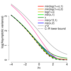
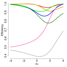
Figure 1: Log of asymptotic variance and efficiency w.r.t. the Cramér-Rao bound for $\hat{\mu}_{h}$ ($\sigma^{2}=1$ known).

Figure 1 shows the theoretical asymptotic variance of $\hat{\mu}_{h}$ as given in Example 5, with $\sigma=1$ known. Efficiency curves measured by the Cramér-Rao lower bound divided by the asymptotic variance are also shown. We see that two truncated versions of $\log(1+x)$ have asymptotic variance close to the Cramér-Rao bound. This asymptotic variance is also reflective of the variance for small finite samples.

Figure 2 is an analog of Figure 1 for $\hat{\sigma}^{2}_{h}$ assuming $\mu=0.5$. For demonstration we choose a nonzero $\mu$ since when $\mu=0$ one can simply use the sample variance (degree of freedom unadjusted) which achieves the Cramér-Rao bound.

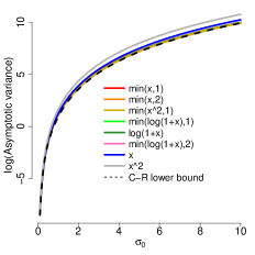
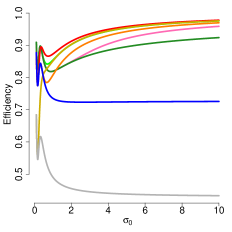
Figure 2: Log of asymptotic variance and efficiency w.r.t. the Cramér-Rao bound for $\hat{\sigma}_{h}^{2}$ ($\mu=0.5$ known).

Here, the truncated versions of $x$ and $x^{2}$ have similar performance when $\sigma$ is not too small. In fact, when $\sigma$ is small, the truncation effect is small and one does not lose much by using the sample variance.

4 REGULARIZED GENERALIZED SCORE MATCHING

We now turn to high-dimensional problems, where the number of parameters $r$ is larger than the sample size $n$. Targeting sparsity in the parameter $\bm{\theta}$, we consider $\ell_{1}$ regularization (Tibshirani, 1996), which has also been used in graphical model estimation (Meinshausen and Bühlmann, 2006; Yuan and Lin, 2007; Voorman et al., 2013).

Definition 8.

Assume the data matrix $\mathbf{x}\in\mathbb{R}^{n\times m}$ comprises $n$ i.i.d. samples from distribution $P_{0}$ with density $p_{0}$ that belongs to an exponential family $\{p_{\bm{\theta}}:\bm{\theta}\in\bm{\Theta}\}\subset\mathcal{P}_{+}$, where $\bm{\Theta}\in\mathbb{R}^{r}$. Define the regularized generalized $\bm{h}$-score matching estimator as

$$\hat{\bm{\theta}}\,\in \operatorname*{argmin}\limits_{\bm{\theta}\in\bm{\Theta}}\hat{J}_{\bm{h},r}(\bm{\theta})$$ (7)

$$\equiv \operatorname*{argmin}\limits_{\bm{\theta}\in\bm{\Theta}}\frac{1}{2}\bm{\theta}^{\top}\bm{\Gamma}(\mathbf{x})\bm{\theta}-\bm{g}(\mathbf{x})^{\top}\bm{\theta}+\lambda\|\bm{\theta}\|_{1},$$

where $\lambda\geq 0$ is a tuning parameter, and $\bm{\Gamma}$ and $\bm{g}$ are from (6).

Discussion of the general conditions for almost sure uniqueness of the solution is omitted here, but in practice we multiply the diagonals of $\bm{\Gamma}$ by a constant slightly larger than $1$ that ensures strict convexity and thus uniqueness of solution. Details about estimation consistency after this operation will be presented in future work. When the solution is unique, the solution path is piecewise linear; compare Lin et al. (2016).

4.1 Truncated GGMs

Using notation from the introduction, let $\bm{X}\sim\mathrm{TN}(\bm{\mu},\mathbf{K})$ be a truncated normal random vector with mean parameter $\bm{\mu}$ and inverse covariance/precision matrix parameter $\mathbf{K}$. Recall that the conditional independence graph for $\bm{X}$ corresponds to the support of $\mathbf{K}$, defined as $S\equiv S(\mathbf{K})\equiv\{(i,j):\kappa_{ij}\neq 0\}$. This support is our target of estimation.

4.2 Truncated Centered GGMs

Consider the case where the mean parameter is zero, i.e., $\bm{\mu}\equiv\bm{0}$, and we want to estimate the inverse covariance matrix $\mathbf{K}\in\mathbb{R}^{m^{2}}$. Assume that for all $j$ there exist constants $M_{j}$ and $M_{j}^{\prime}$ that bound $h_{j}$ and its derivative $h_{j}^{\prime}$ a.e. Assume further that $h_{j}(x)>0$ a.e, $\lim_{x\searrow 0^{+}}h_{j}(x)=0$, and $h_{j}^{\prime}(x)\geq 0$. Boundedness here is for ease of proof in the main theorems; reasonable choices of unbounded $h$ are also valid. Then, (A1)–(A2) are satisfied, and the loss can be written as

$$\hat{J}_{r+}(\mathbf{K})=\tfrac{1}{2}\mathrm{vec}(\mathbf{K})^{\top}\bm{\Gamma}(\mathbf{x})\mathrm{vec}(\mathbf{K})\\ -\bm{g}(\mathbf{x})^{\top}\mathrm{vec}(\mathbf{K})+\lambda\|\mathbf{K}\|_{1},$$ (8)

with the $j^{\mathrm{th}}$ block of the $m^{2}\times m^{2}$ block-diagonal matrix $\bm{\Gamma}(\mathbf{x})$ being

$$n^{-1}\mathbf{x}^{\top}\mathrm{diag}(\bm{h}_{j}(\bm{X}_{j}))\mathbf{x},$$

where $\bm{h}_{j}(\bm{X}_{j})\equiv[h_{j}(X_{j}^{(1)}),\ldots,h_{j}(X_{j}^{(n)})]^{\top}$, $\mathrm{diag}(c_{1},\ldots,c_{n})$ denotes a diagonal matrix with diagonal entries $c_{1},\ldots,c_{n}$, and

$$\bm{g}(\mathbf{x}) \equiv\mathrm{vec}(\mathbf{u})+\mathrm{vec}(\mathrm{diag}(\bm{V})),\, \,\,\mathbf{u}\equiv n^{-1}\mathbf{h^{\prime}}(\mathbf{x})^{\top}\mathbf{x},$$

$$\bm{V} \equiv n^{-1}\mathbf{h}(\mathbf{x})^{\top}\mathbf{1}_{n},\, \,\,\mathbf{h}(\mathbf{x})\equiv[h_{j}(X_{j}^{(i)})]_{i,j},$$

$$\mathbf{h^{\prime}}(\mathbf{x}) \equiv[h^{\prime}_{j}(X_{j}^{(i)})]_{i,j},\, \,\,\mathbf{1}_{n}=[1,\ldots,1]^{\top}.$$

The regularized generalized $\bm{h}$-score matching estimator of $\mathbf{K}$ in the truncated centered GGM is

$$\hat{\mathbf{K}}\equiv\operatorname*{argmin}_{\begin{subarray}{c}\mathbf{K}\in\mathbb{R}^{m^{2}},\mathbf{K}=\mathbf{K}^{\top}\end{subarray}}\hat{J}_{r+}(\mathbf{K}),$$ (9)

where $\bm{\Gamma}(\mathbf{x})$ and $\bm{g}(\mathbf{x})$ are defined above.

Definition 9.

For true inverse covariance matrix $\mathbf{K}_{0}$, let $\bm{\Gamma}_{0}\equiv\mathbb{E}_{0}\bm{\Gamma}(\mathbf{x})$ and $\bm{g}_{0}\equiv\mathbb{E}_{0}\bm{g}(\mathbf{x})$. Denote the support of a precision matrix $\mathbf{K}$ as $S\equiv S(\mathbf{K})\equiv\{(i,j):\kappa_{ij}\neq 0\}.$ Write the true support of $\mathbf{K}_{0}$ as $S_{0}=S(\mathbf{K}_{0})$. Suppose the maximum number of non-zero entries in rows of $\mathbf{K}_{0}$ is $d_{\mathbf{K}_{0}}$. Let $\mathbf{\Gamma}_{SS}$ be the entries of $\mathbf{\Gamma}\in\mathbb{R}^{m^{2}\times m^{2}}$ corresponding to edges in $S$. Define

$$c_{\bm{\Gamma}_{0}}\equiv{|\kern-1.07639pt|\kern-1.07639pt|(\bm{\Gamma}_{0,S_{0}S_{0}})^{-1}|\kern-1.07639pt|\kern-1.07639pt|}_{\infty,\infty},\quad c_{\bm{K}_{0}}\equiv{|\kern-1.07639pt|\kern-1.07639pt|\mathbf{K}_{0}|\kern-1.07639pt|\kern-1.07639pt|}_{\infty,\infty}.$$

We say the irrepresentability condition holds for $\bm{\Gamma}_{0}$ if there exists an $\alpha\in(0,1]$ such that

$${|\kern-1.07639pt|\kern-1.07639pt|\bm{\Gamma}_{0,S_{0}^{c}S_{0}}(\bm{\Gamma}_{0,S_{0}S_{0}})^{-1}|\kern-1.07639pt|\kern-1.07639pt|}_{\infty,\infty}\leq(1-\alpha).$$ (10)

Theorem 10.

Suppose $\bm{X}\sim\mathrm{TN}(\bm{0},\mathbf{K}_{0})$ and $\bm{h}$ is as discussed in the opening paragraph of this section. Suppose further that $\bm{\Gamma}_{0,S_{0}S_{0}}$ is invertible and satisfies the irrepresentability condition (10) with $\alpha\in(0,1]$. Let $\tau>3$. If the sample size and the regularization parameter satisfy

$$n \geq\mathcal{O}\left(d_{\mathbf{K}_{0}}^{2}\tau\log m\max\left\{\frac{c_{\bm{\Gamma}_{0}}^{2}c_{\bm{X}}^{4}}{\alpha^{2}},1\right\}\right),$$ (11)

$$\lambda >\mathcal{O}\left[(c_{\mathbf{K}_{0}}c_{\bm{X}}^{2}+c_{\bm{X}}+1)\left(\sqrt{\frac{\tau\log m}{n}}+\frac{\tau\log m}{n}\right)\right],$$ (12)

where $c_{\bm{X}}\equiv 2\max_{j}\left(2\sqrt{(\mathbf{K}_{0}^{-1})_{jj}}+\sqrt{e}\mathbb{E}_{0}X_{j}\right)$, then the following statements hold with probability $1-m^{3-\tau}$:

1. The regularized generalized $\bm{h}$-score matching estimator $\hat{\mathbf{K}}$ defined in (9) is unique, has its support included in the true support, $\hat{S}\equiv S(\hat{\mathbf{K}})\subseteq S_{0}$, and

   $$\|\hat{\mathbf{K}}-\mathbf{K}_{0}\|_{\infty} <\frac{c_{\bm{\Gamma}_{0}}}{2-\alpha}\lambda,$$

   $${|\kern-1.07639pt|\kern-1.07639pt|\hat{\mathbf{K}}-\mathbf{K}_{0}|\kern-1.07639pt|\kern-1.07639pt|}_{F} \leq\frac{c_{\bm{\Gamma}_{0}}}{2-\alpha}\lambda\sqrt{|S_{0}|},$$

   $${|\kern-1.07639pt|\kern-1.07639pt|\hat{\mathbf{K}}-\mathbf{K}_{0}|\kern-1.07639pt|\kern-1.07639pt|}_{2} \leq\frac{c_{\bm{\Gamma}_{0}}}{2-\alpha}\lambda\min(\sqrt{|S_{0}|},d_{\mathbf{K}_{0}}).$$

2. Moreover, if

   $$\min_{j,k}|\kappa_{0,jk}|>\frac{c_{\bm{\Gamma}_{0}}}{2-\alpha}\lambda,$$

   then $\hat{S}=S_{0}$ and $\mathrm{sign}(\hat{\kappa}_{jk})=\mathrm{sign}(\kappa_{0,jk})$ for all $(j,k)\in S_{0}$.

The theorem is proved in the supplement. A key ingredient of the proof is a tail bound on $\|\bm{\Gamma}-\bm{\Gamma}_{0}\|_{\infty}$, which is composed of products of the $X_{j}^{(i)}$’s. In Lin et al. (2016), the products are up to fourth moments. Using a bounded $\bm{h}$ our products automatically calibrate to a quadratic polynomial when the observed values are large, and resort to higher moments only when they are small. Using this scaling, we obtain improved bounds and convergence rates, underscored in the new requirement on the sample size $n$, which should be compared to $n>\mathcal{O}((\log m^{\tau})^{8})$ in Lin et al. (2016).

4.3 Truncated Non-centered GGMs

Suppose now $\bm{X}\sim\mathrm{TN}(\bm{\mu}_{0},\mathbf{K}_{0})$ with both $\bm{\mu}_{0}$ and $\mathbf{K}_{0}$ unknown. While our main focus is still on the inverse covariance parameter $\mathbf{K}$, we now also have to estimate a mean parameter $\bm{\mu}$. Instead, we estimate the canonical parameters $\mathbf{K}$ and $\bm{\eta}\equiv\mathbf{K}\bm{\mu}$. Concatenating $\bm{\Xi}\equiv[\mathbf{K},\bm{\eta}]$, the corresponding $\bm{h}$-score matching loss has a similar form to (8) and (9) with $\mathbf{K}$ replaced by $\bm{\Xi}$, and different $\bm{\Gamma}$ and $\bm{g}$. As a corollary of the centered case, we have an analogous bound on the error in the resulting estimator $\hat{\bm{\Xi}}$; we omit the details here. We note, however, that we can have different tuning penalty parameters $\lambda_{\mathbf{K}}$ and $\lambda_{\bm{\eta}}$ for $\mathbf{K}$ and $\bm{\eta}$, respectively, as long as their ratio is fixed, since we can scale the $\bm{\eta}$ parameter by the ratio accordingly. To avoid picking two tuning parameters, one may also choose to remove the penalty on $\bm{\eta}$ altogether by profiling out $\bm{\eta}$. We leave a detailed analysis of the profiled estimator to future research.

4.4 Tuning Parameter Selection

By treating the loss as the mean negative log-likelihood, we may use the extended Bayesian information Criterion (eBIC) to choose the tuning parameter (Chen and Chen, 2008; Foygel and Drton, 2010). Let $\hat{S}^{\lambda}\equiv\{(i,j):\hat{\kappa}_{ij}^{\lambda}\neq 0,i<j\}$, where $\hat{\mathbf{K}}^{\lambda}$ be the estimate associated with tuning parameter $\lambda$. The eBIC is then

$$\mathrm{eBIC}(\lambda)=-n\mathrm{vec}(\hat{\mathbf{K}})^{\top}\bm{\Gamma}(\mathbf{x})\mathrm{vec}(\hat{\mathbf{K}})\\ +2n\bm{g}(\mathbf{x})^{\top}\mathrm{vec}(\hat{\mathbf{K}})+|\hat{S}^{\lambda}|\log n+2\log\left(\begin{matrix}p(p-1)/2\\ |\hat{S}^{\lambda}|\end{matrix}\right),$$

where $\hat{\mathbf{K}}$ can be either the original estimate associated with $\lambda$, or a refitted solution obtained by restricting the support to $\hat{S}^{\lambda}$.

5 NUMERICAL EXPERIMENTS

We present simulation results for non-negative GGM estimators with different choices of $\bm{h}$. We use a common $h$ for all columns of the data matrix $\mathbf{x}$. Specifically, we consider functions such as $h_{j}(x)=x$ and $h_{j}(x)=\log(1+x)$ as well as truncations of these functions. In addition, we try MCP (Fan and Li, 2001) and SCAD penalty-like (Zhang, 2010) functions.

5.1 Implementation

We use a coordinate-descent method analogous to Algorithm 2 in Lin et al. (2016), where in each step we update each element of $\hat{\mathbf{K}}$ based on the other entries from the previous steps, while maintaining symmetry. Warm starts using the solution from the previous $\lambda$, as well as lasso-type strong screening rules (Tibshirani et al., 2012) are used for speedups. In our simulations below we always scaled the data matrix by column $\ell_{2}$ norms before proceeding to estimation.

5.2 Truncated Centered GGMs

For data from a truncated centered Gaussian distribution, we compared our truncated centered Gaussian estimator (9) with various choices of $h$, to SpaCE JAM (SJ, Voorman et al., 2013), which estimates graphs without assuming a specific form of distribution, a pseudo-likelihood method SPACE (Peng et al., 2009) with CONCORD reformulation (Khare et al., 2015), graphical lasso (Yuan and Lin, 2007; Friedman et al., 2008), the neighborhood selection estimator (NS) in Meinshausen and Bühlmann (2006), and finally nonparanormal SKEPTIC (Liu et al., 2012) with Kendall’s $\tau$. While we ran all these competitors, only the top performing methods are explicitly shown in our reported results. Recall that the choice of $h(x)=x^{2}$ corresponds to the estimator in Lin et al. (2016), using score matching from Hyvärinen (2007).

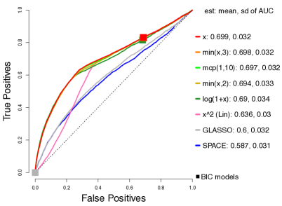
Figure 3: Average ROC curves of our estimator with various choices of $h$, compared to SPACE and GLASSO, for the truncated centered Gaussian case. $n=80$, $m=100$. Squares indicate average true positive rate (TPR) and false positive rate (FPR) of models picked by eBIC (with refitting) for the estimator in the same color. eBIC is introduced in Section 4.4.

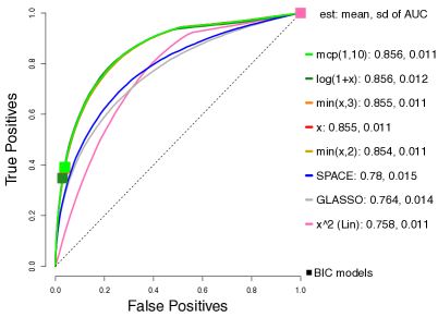
Figure 4: Same setting as in Figure 3, with $n=1000$.

A few representative ROC (receiver operating characteristic) curves for edge recovery are plotted in Figures 3 and 4, using $m=100$ and $n=80$ or $n=1000$, respectively. Each curve corresponds to the average of 50 ROCs obtained from estimation of $\mathbf{K}$ from $\mathbf{x}$ generated using 5 different true precision matrices $\mathbf{K}_{0}$, each with 10 trials. The averaging method is mean AUC-preserving and is introduced as vertical averaging and outlined in Algorithm 3 in Fawcett (2006). The construction of $\mathbf{K}_{0}$ is the same as in Section 4.2 of Lin et al. (2016): a graph with $m=100$ nodes with 10 disconnected subgraphs containing the same number of nodes, i.e. $\mathbf{K}_{0}$ is block-diagonal. In each sub-matrix, we generate each lower triangular element to be $0$ with probability $\pi\in(0,1)$, and from a uniform distribution on interval $[0.5,1]$ with probability $1-\pi$. The upper triangular elements are set accordingly by symmetry. The diagonal elements of $\mathbf{K}_{0}$ are chosen to be a common positive value so that the minimum eigenvalue of $\mathbf{K}_{0}$ is $0.1$. We choose $\pi=0.2$ for $n=80$ and $\pi=0.8$ for $n=1000$.

For clarity, we only plot some top-performing representatives of the functions we considered. However, all of the alternative functions $h$ we considered perform better than $h(x)=x^{2}$ from Hyvärinen (2007) and Lin et al. (2016).

5.3 Truncated Non-Centered GGMs

Next we generate data from a truncated non-centered Gaussian distribution with both parameters $\bm{\mu}$ and $\mathbf{K}$ unknown. Consider $\hat{\mathbf{K}}$ as part of the estimated $\hat{\bm{\Xi}}$ as discussed in Section 4.3. In each trial we form the true $\mathbf{K}_{0}$ as in Section 5.2, and we generate each component of $\bm{\mu}_{0}$ independently from the normal distribution with mean $0$ and standard deviation $0.5$.

As discussed in Section 4.3, we assume the ratio of the tuning parameters for $\mathbf{K}$ and $\bm{\eta}$ to be fixed. Shown in Figure 5 are average ROC curves (over 50 trials as in Section 5.2) for truncated non-centered GGM estimators with $h(x)=\min(x,3)$; each curve corresponds to a different ratio ${\lambda_{\mathbf{K}}}/{\lambda_{\bm{\eta}}}$, where “Inf” indicates $\lambda_{\bm{\eta}}\equiv 0$. Here, $n=1000$ and $m=100$.

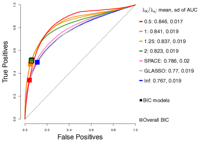
Figure 5: Performance of the non-centered estimator with $h(x)=\min(x,3)$; each curve corresponds to a different choice of fixed $\lambda_{\mathbf{K}}/\lambda_{\bm{\eta}}$. $n=1000$, $m=100$.

Clearly, as the ratio increases, the performance improves, and after a certain threshold it deteriorates. The AUC for the profiled estimator with $\lambda_{\bm{\eta}}=0$ is among the worst, so there indeed is a lot to be gained from tuning an extra tuning parameter, although there is a tradeoff between time and performance.

In Figure 6 we compare the performance of the profiled estimator with different $h$, to SPACE and GLASSO, each with 50 trials as before. It can be seen that even without tuning the extra parameter, the estimators, except for $h(x)=x^{2}$, still work as well as SPACE and GLASSO, and outperform Lin et al. (2016).

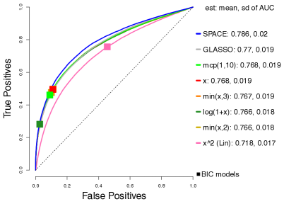
Figure 6: Performance of the non-centered profiled estimators using various $h$, $n=1000$, $m=100$.

6 DISCUSSION

In this paper we proposed a generalized version of the score matching estimator of Hyvärinen (2007) which avoids the calculation of normalizing constants. For estimation of the canonical parameters of exponential families, our generalized loss retains the nice property of being quadratic in the parameters. Our estimator offers improved estimation properties through various scalar or vector-valued choices of function $\bm{h}$.

For high-dimensional exponential family graphical models, following the work of Meinshausen and Bühlmann (2006), Yuan and Lin (2007) and Lin et al. (2016), we add an $\ell_{1}$ penalty to the generalized score matching loss, giving a solution that is almost surely unique under regularity conditions and has a piecewise linear solution path.

In the case of multivariate truncated Gaussian distribution, where the conditional independence graph is given by the inverse covariance parameter, the sample size required for the consistency of our method is $\Omega(d^{2}\log m)$, where $m$ is the dimension and $d$ is the maximum node degree in the corresponding independence graph. This matches the rates for GGMs in Ravikumar et al. (2011) and Lin et al. (2016), and lasso with linear regression (Bühlmann and van de Geer, 2011).

A potential problem for future work would be adaptive choice of the function $\bm{h}$ from data, or to develop a summary score similar to eBIC that can be used to compare not just different tuning parameters but also across different models.

References

See pages - of Supp

References

- Bühlmann and van de Geer (2011) P. Bühlmann and S. van de Geer. Statistics for high-dimensional data: methods, theory and applications. Springer Science & Business Media, 2011.
- Chen and Chen (2008) J. Chen and Z. Chen. Extended Bayesian information criteria for model selection with large model spaces. Biometrika, 95(3):759–771, 2008.
- Chen et al. (2014) S. Chen, D. M. Witten, and A. Shojaie. Selection and estimation for mixed graphical models. Biometrika, 102(1):47–64, 2014.
- Dobra and Lenkoski (2011) A. Dobra and A. Lenkoski. Copula Gaussian graphical models and their application to modeling functional disability data. The Annals of Applied Statistics, 5(2A):969–993, 2011.
- Drton and Maathuis (2017) M. Drton and M. H. Maathuis. Structure learning in graphical modeling. Annual Review of Statistics and Its Application, 4:365–393, 2017.
- Drton and Perlman (2004) M. Drton and M. D. Perlman. Model selection for Gaussian concentration graphs. Biometrika, 91(3):591–602, 2004.
- Fan and Li (2001) J. Fan and R. Li. Variable selection via nonconcave penalized likelihood and its oracle properties. Journal of the American Statistical Association, 96(456):1348–1360, 2001.
- Fawcett (2006) T. Fawcett. An introduction to ROC analysis. Pattern Recognition Letters, 27(8):861–874, 2006.
- Fellinghauer et al. (2013) B. Fellinghauer, P. Bühlmann, M. Ryffel, M. Von Rhein, and J. D. Reinhardt. Stable graphical model estimation with random forests for discrete, continuous, and mixed variables. Computational Statistics & Data Analysis, 64:132–152, 2013.
- Foygel and Drton (2010) R. Foygel and M. Drton. Extended Bayesian information criteria for Gaussian graphical models. In Advances in Neural Information Processing Systems, pages 604–612, 2010.
- Friedman et al. (2008) J. Friedman, T. Hastie, and R. Tibshirani. Sparse inverse covariance estimation with the graphical lasso. Biostatistics, 9(3):432–441, 2008.
- Hyvärinen (2005) A. Hyvärinen. Estimation of non-normalized statistical models by score matching. Journal of Machine Learning Research, 6(4), 2005.
- Hyvärinen (2007) A. Hyvärinen. Some extensions of score matching. Computational Statistics & Data Analysis, 51(5):2499–2512, 2007.
- Khare et al. (2015) K. Khare, S.-Y. Oh, and B. Rajaratnam. A convex pseudolikelihood framework for high dimensional partial correlation estimation with convergence guarantees. Journal of the Royal Statistical Society: Series B (Statistical Methodology), 77(4):803–825, 2015.
- Lauritzen (1996) S. L. Lauritzen. Graphical models, volume 17. Clarendon Press, 1996.
- Lin et al. (2016) L. Lin, M. Drton, and A. Shojaie. Estimation of high-dimensional graphical models using regularized score matching. Electronic Journal of Statistics, 10(1):806–854, 2016.
- Liu et al. (2009) H. Liu, J. Lafferty, and L. Wasserman. The nonparanormal: Semiparametric estimation of high dimensional undirected graphs. Journal of Machine Learning Research, 10(Oct):2295–2328, 2009.
- Liu et al. (2012) H. Liu, F. Han, M. Yuan, J. Lafferty, L. Wasserman, et al. High-dimensional semiparametric gaussian copula graphical models. The Annals of Statistics, 40(4):2293–2326, 2012.
- Meinshausen and Bühlmann (2006) N. Meinshausen and P. Bühlmann. High-dimensional graphs and variable selection with the lasso. Ann. Statist., 34(3):1436–1462, 2006.
- Parry et al. (2012) M. Parry, A. P. Dawid, and S. Lauritzen. Proper local scoring rules. The Annals of Statistics, 40(1):561–592, 2012.
- Peng et al. (2009) J. Peng, P. Wang, N. Zhou, and J. Zhu. Partial correlation estimation by joint sparse regression models. Journal of the American Statistical Association, 104(486):735–746, 2009.
- Ravikumar et al. (2010) P. Ravikumar, M. J. Wainwright, and J. D. Lafferty. High-dimensional Ising model selection using -regularized logistic regression. Ann. Statist., 38(3):1287–1319, 2010.
- Ravikumar et al. (2011) P. Ravikumar, M. J. Wainwright, G. Raskutti, and B. Yu. High-dimensional covariance estimation by minimizing -penalized log-determinant divergence. Electronic Journal of Statistics, 5:935–980, 2011.
- Tibshirani (1996) R. Tibshirani. Regression shrinkage and selection via the lasso. Journal of the Royal Statistical Society. Series B (Methodological), pages 267–288, 1996.
- Tibshirani et al. (2012) R. Tibshirani, J. Bien, J. Friedman, T. Hastie, N. Simon, J. Taylor, and R. J. Tibshirani. Strong rules for discarding predictors in lasso-type problems. Journal of the Royal Statistical Society: Series B (Statistical Methodology), 74(2):245–266, 2012.
- Voorman et al. (2013) A. Voorman, A. Shojaie, and D. Witten. Graph estimation with joint additive models. Biometrika, 101(1):85–101, 2013.
- Yang et al. (2015) E. Yang, P. Ravikumar, G. I. Allen, and Z. Liu. Graphical models via univariate exponential family distributions. Journal of Machine Learning Research, 16(1):3813–3847, 2015.
- Yu et al. (2016) M. Yu, M. Kolar, and V. Gupta. Statistical inference for pairwise graphical models using score matching. In Advances in Neural Information Processing Systems, pages 2829–2837, 2016.
- Yuan and Lin (2007) M. Yuan and Y. Lin. Model selection and estimation in the Gaussian graphical model. Biometrika, 94(1):19–35, 2007.
- Zhang (2010) C.-H. Zhang. Nearly unbiased variable selection under minimax concave penalty. The Annals of Statistics, 38(2):894–942, 2010.