CGC/saturation approach: an impact-parameter dependent model for diffraction production in DIS.

Abstract

In the paper we discussed the evolution equations for diffractive production in the framework of CGC/saturation approach, and found the analytical solutions for several kinematic regions. The most impressive features of these solutions are, that diffractive production does not exibit geometric scaling behaviour i.e. being a function of one variable.

Based on these solutions, we suggest an impact parameter dependent saturation model, which is suitable for describing diffraction production both deep in the saturation region, and in the vicinity of the saturation scale.

Using the model we attempted to fit the combined data on diffraction production from H1 and ZEUS collaborations. We found that we are able describe both $x_{I\!\!P}$ and $\beta$ dependence, as well as $Q$ behavior of the measured cross sections. In spite of the sufficiently large $\chi^{2}/d.o.f.$ we believe that our description provides an initial impetus to find a fit of the experimental data, based on the solution of the CGC/saturation equation, rather than on describing the diffraction system in simplistic manner, assuming that only quark-antiquark pair and one extra gluons, are produced.

I Introduction.

In this paper we discuss diffractive production in the deep inelastic scattering in the framework of CGC/saturation approach (see Ref.KOLEB for review). In spite of the fact that the equations for the diffractive production in this approach, were proven long ago KOLE (see also Ref.HWS ; HIMST ; KLW ) the intensive study, during the past two decades, has been concentrated on the simplified model in which the diffractive production of quark-antiquark pair and one additional gluon has been considered (see Refs.GBKW ; GOLEDD ; SATMOD0 ; KOML ; MUSCH ; MASC ; MAR ; KLMV ). Such models described the experimental data quite well, giving the impression that we do not need to search for the solution of the general equations. Indeed, we found only two attempts to solve the equations of Ref.KOLE numerically (see Refs,LELUDD ; LELUDD1 ).

The main goal of this paper is to investigate the non-linear equations for diffractive production in DIS, and to find an analytical solution in different kinematic regions. Based on these analytical solutions we will suggest an impact parameter dependent model in the spirit of Refs.CLP1 ; CLP which is based on Color Glass Condensate/saturation effective theory for high energy QCD.

The paper consists of two parts. In the first part, which is the most important contribution in this paper, we found the analytical solutions of the evolution equations for diffraction productionKOLE in different kinematic regions, mostly using the approach developed in Ref.LETU . In the second part of the paper, we suggest an interpolation formula which satisfies two limits found analytically: deep in the saturation region, and in the vicinity of the saturation scale, putting into practice the key ideas of Ref.IIM . This formula exhibits the main features of the DIS amplitude , given in Refs.CLP1 ; CLP ; CLM , but it is different from the interpolation procedure that have been used in numerous attempts to build a such model in Refs. IIM ; SATMOD0 ; SATMOD1 ; BKL ; SATMOD2 ; SATMOD3 ; SATMOD4 ; SATMOD5 ; SATMOD6 ; SATMOD7 ; SATMOD8 ; SATMOD9 ; SATMOD10 ; SATMOD11 ; SATMOD12 ; SATMOD13 ; SATMOD14 ; SATMOD15 ; SATMOD16 ; SATMOD17 . We will attempt to describe the HERA data in the region of small $x_{I\!\!P}$ and small $\beta$.HERADATA .

Unfortunately, we are still doomed to build models to introduce the main features of the CGC/saturation approach, since the CGC/saturation equations do not reproduce the correct behavior of the scattering amplitude at large impact parameter (see Ref. KW ; FIIM ). Real progress in theoretical understanding of the confinement of quarks and gluon has not yet been achieved and, as a result, we do not know how to formulate the CGC/saturation equations to incorporate the phenomenon of confinement. We have to build a model which includes both the theoretical knowledge that stems from the CGC/saturation equations, and the phenomenological large $b$ behavior that does not contradict theoretical restrictions FROI ; BRLE . In our modeling of the large $b$ behaviour of the scattering amplitude, we follow the main ideas of all saturation models on the market (see for example Refs.IIM ; SATMOD0 ; SATMOD1 ; BKL ; SATMOD2 ; SATMOD3 ; SATMOD4 ; SATMOD5 ; SATMOD6 ; SATMOD7 ; SATMOD8 ; SATMOD9 ; SATMOD10 ; SATMOD11 ; SATMOD12 ; SATMOD13 ; SATMOD14 ; SATMOD15 ; SATMOD16 ; SATMOD17 ): and only introduce the non-perturbative behaviour in the $b$-dependence of the saturation scale.

For the $b$ behavior we use the procedure, suggested in Ref. CLP :

$$Q^{2}_{s}\left(Y,b\right)\,=\,Q^{2}_{0}\left(S\left(b,m\right)\right)^{\frac{1}{\bar{\gamma}}}\,e^{\lambda\,Y}$$ (1)

where $S\left(b\right)$ is the Fourier image of $S\left(Q_{T}\right)=1/\left(1+\frac{Q^{2}_{T}}{m^{2}}\right)^{2}$, and we will discuss below the value of $\bar{\gamma}$. Eq. (1) leads to the scattering amplitude which is proportional $\exp\left(-mb\right)$ at $b\gg 1/m$ in accord with the Froissart theorem FROI . In addition, we reproduce the large $Q_{T}$ dependence of this amplitude, which is proportional to $Q^{-4}_{T}$ and follows from the perturbative QCD calculation BRLE . This impact parameter behaviour is the main phenomenological assumption that we used.

II Theoretical input

In this section we discuss our theoretical input that follows from the Colour Glass Condensate(CGC)/saturation effective theory of QCD at high energies(see Ref.KOLEB for the basic introduction).

II.1 The evolution equation for diffraction production in the framework of CGC.

A sketch of the process of diffraction production in DIS is shown in Fig. 1-c, from this figure one can see that the main formula takes the form

$$\sigma^{\rm diff}(Y,Y_{0},Q^{2})\,\,\,=\,\,\int\,\,d^{2}r_{\perp}\int\,dz\,\,|\Psi^{\gamma^{*}}(Q^{2};r_{\perp},z)|^{2}\,\,\sigma_{\rm dipole}^{diff}(r_{\perp},Y,Y_{0})\,,$$ (2)

where $Y=\ln\left(1/x_{Bj}\right)$ and $Y_{0}$ is the minimum rapidity gap for the diffraction process (see Fig. 1-c). In other words, we consider diffraction production, in which all produced hadrons have rapidities larger than $Y_{0}$. For $\sigma_{\rm dipole}^{diff}(r_{\perp},Y,Y_{0})$ we have a general expression

$$\sigma_{\rm dipole}^{diff}(r_{\perp},Y,Y_{0})\,\,=\,\,\,\,\int\,d^{2}b\,d^{2}b^{\prime}\,N^{D}(r_{\perp},Y,Y_{0};\boldsymbol{b})\,,$$ (3)

where the structure of the amplitude $N^{D}$ is shown in Fig. 1-a.

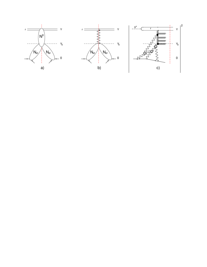
Figure 1: The graphic representation of the processes of diffraction production

For $N^{D}$ the evolution equation has been derived in Ref.KOLE in the leading log(1/x) approximation (LLA) of perturbative QCD(see Ref.KOLEB for details and general descriptions of the LLA). Hence, we hope to describe the experimental data only in the kinematic region where both $\beta$ and $x_{I\!\!P}$ are very small ($Y-Y_{0}\,=\,\ln(1/\beta)\,\gg\,1$ and $Y_{0}=\ln(1/x_{pom}\,gg\,1$ are large. We are aware, that it is sufficient to describe most of th experimental data by only taking into account $q\bar{q}$ and $q\bar{q}G$ final states in diffraction production. Because of this, our main goal is not to describe the current experiments, but to study the solution to the equations in the LLA, which introduces the screening corrections to all the channels of the diffraction production. By comparing with the experimental data, we wish to determine in which kinematic region the shadowing corrections will become important, both for the elastic amplitudes in Fig. 1, as well as for the diffractive production of the large number of gluons.

The equation as has been shown in Ref.KOLE , can be written in two forms. First, it turns out that for the new function

$${\cal N}\left(Y,Y_{0};r_{\perp},b\right)\,\,\equiv\,\,2N_{\rm el}\left(Y;r_{\perp},b\right)\,\,-\,\,N^{D}(r_{\perp},x,x_{0};b)$$ (4)

the equation has the same form as Balitsky-Kovchegov equationBK : viz.

$$\displaystyle{\frac{\partial{\cal N}\left(Y,Y_{0};\boldsymbol{x}_{01},\boldsymbol{b}\right)}{\partial Y}}\, = \,\displaystyle{\frac{\bar{\alpha}_{S}}{\pi}\int d^{2}{\mathbf{x_{2}}}\frac{{\mathbf{x^{2}_{01}}}}{{\mathbf{x^{2}_{02}}}\,{\mathbf{x^{2}_{12}}}}\Bigg{\{}{\cal N}\left(Y,Y_{0};\boldsymbol{x}_{02},\boldsymbol{b}-\frac{1}{2}\boldsymbol{x}_{12}\right)+{\cal N}\left(Y,Y_{0};\boldsymbol{x}_{12},\boldsymbol{b}-\frac{1}{2}\boldsymbol{x}_{02}\right)\,-\,{\cal N}\left(Y,Y_{0};\boldsymbol{x}_{01},\boldsymbol{b}\right)}\,$$ (5)

$$- \,\displaystyle{{\cal N}\left(Y,Y_{0};\boldsymbol{x}_{02},\boldsymbol{b}-\frac{1}{2}\boldsymbol{x}_{12}\right){\cal N}\left(Y,Y_{0};\boldsymbol{x}_{12},\boldsymbol{b}-\frac{1}{2}\boldsymbol{x}_{02}\right)\Bigg{\}}}$$

Note, that $\boldsymbol{r}=\boldsymbol{x}_{01}$ and the kernel of the equation describe the decay of a dipole to two dipoles: $\boldsymbol{x}_{01}\,\to\,\boldsymbol{x}_{02}\,+\,\boldsymbol{x}_{12}$. The initial condition for Eq. (5) has the following form:

$${\cal N}\left(Y=Y_{0},Y_{0};\boldsymbol{x}_{01},\boldsymbol{b}\right)\,\,=\,\,2\,N_{\rm el}\left(Y=Y_{0};\boldsymbol{x}_{01},\boldsymbol{b}\right)\,-\,N^{2}_{\rm el}\left(Y=Y_{0};\boldsymbol{x}_{01},\boldsymbol{b}\right)$$ (6)

Re-writing Eq. (5) as the equation for $N^{D}$ we obtain the second form of the set of the equations:

$$\frac{\partial N^{D}\left(Y,Y_{0};\boldsymbol{x}_{01},\boldsymbol{b}\right)}{\partial Y}\,=$$ (7)

$$\,\frac{\bar{\alpha}_{S}}{\pi}\int\,d^{2}\boldsymbol{x}_{2}\frac{{\mathbf{x^{2}_{01}}}}{{\mathbf{x^{2}_{02}}}\,{\mathbf{x^{2}_{12}}}}\Bigg{\{}\,N^{D}\left(Y,Y_{0};\boldsymbol{x}_{02},\boldsymbol{b}-\frac{1}{2}\boldsymbol{x}_{12}\right)+N^{D}\left(Y,Y_{0};\boldsymbol{x}_{12},\boldsymbol{b}-\frac{1}{2}\boldsymbol{x}_{02}\right)\,-\,N^{D}\left(Y,Y_{0};\boldsymbol{x}_{01},\boldsymbol{b}\right)$$

$$+\,\,N^{D}(Y,Y_{0};\boldsymbol{x}_{02},\boldsymbol{b}-\frac{1}{2}\boldsymbol{x}_{12})N^{D}(Y,Y_{0};\boldsymbol{x}_{12},\boldsymbol{b}-\frac{1}{2}\boldsymbol{x}_{02})-4\,N^{D}(Y,Y_{0};\boldsymbol{x}_{02},\boldsymbol{b}-\frac{1}{2}\boldsymbol{x}_{12})N_{\rm el}(Y;\boldsymbol{x}_{12},\boldsymbol{b}-\frac{1}{2}\boldsymbol{x}_{02})$$

$$+2\,N_{\rm el}(Y;\boldsymbol{x}_{02},\boldsymbol{b}-\frac{1}{2}\boldsymbol{x}_{12})N_{\rm el}(Y;\boldsymbol{x}_{12},\boldsymbol{b}-\frac{1}{2}\boldsymbol{x}_{02})]\,\Bigg{\}}.$$

The initial conditions are

$$N^{D}\left(Y=Y_{0},Y_{0};\boldsymbol{x}_{01},\boldsymbol{b}^{\prime}\right)\,\,=\,\,N^{2}_{\rm el}(Y_{0};\boldsymbol{x}_{01},\boldsymbol{b})$$ (8)

A general feature, is that the amplitude with fixed rapidity gap can be calculate as follows

$$n^{D}\left(Y,\mbox{ rapidity gap}=Y_{0};\boldsymbol{x}_{01},\boldsymbol{b}\right)\,=\,-\frac{\partial N^{D}\left(Y,Y_{0};\boldsymbol{x}_{01},\boldsymbol{b}\right)}{\partial Y_{0}}\,=\,\frac{\partial{\cal N}\left(Y,Y_{0};\boldsymbol{x}_{01},\boldsymbol{b}\right)}{\partial Y_{0}}\,$$ (9)

From Fig. 1 one can see that $n^{D}\left(Y,\mbox{ rapidity gap}=Y_{0};\boldsymbol{x}_{01},\boldsymbol{b}\right)\,\,=\,\,\int d^{2}b^{\prime}{\nu}^{D}\left(Y,\mbox{ rapidity gap}=Y_{0};\boldsymbol{x}_{01},\boldsymbol{b,\boldsymbol{b}^{\,{}^{\prime}}}\right)$ where $\boldsymbol{b}^{\,{}^{\prime}}$ is the conjugate variable to the momentum transfer in Fig. 1 for the amplitudes $N_{el}$.

II.2 $N^{D}$ deep in the saturation region: $r^{2}Q^{2}_{s}\left(Y_{0}\right)\,\gg\,1$ and $r^{2}Q^{2}_{s}\left(Y-Y_{0}\right)\,\gg\,1$, and a violation of the geometric scaling behavior

First, we consider the kinematic region, where $r^{2}Q^{2}_{s}\left(Y_{0}\right)\,\gg\,1$ and $r^{2}Q^{2}_{s}\left(Y-Y_{0}\right)\,\gg\,1$. Note, that $r^{2}Q^{2}_{s}\left(Y\right)\,\gg\,1$ stems from the above restrictions.

In this region where both $Y$ and $Y_{0}$ as well as the difference between them are large, we can expect that both $N^{D}$ and $N_{\rm el}$ are close to 1. Therefore, we can use the procedure suggested in Ref. LETU . In this region we can replace

$${\cal N}^{D}\left(Y,Y_{0},\boldsymbol{x}_{01},\boldsymbol{b}\right)\,\,=\,\,1\,-\,\Delta^{D}\left(Y,Y_{0},\boldsymbol{x}_{01},\boldsymbol{b}\right);~{}~{}~{}~{}~{}~{}~{}~{}~{}~{}~{}~{}N_{\rm el}\left(Y,\boldsymbol{x}_{01},\boldsymbol{b}\right)\,\,=\,\,1\,-\,\Delta_{\rm el}\left(Y,\boldsymbol{x}_{01},\boldsymbol{b}\right);$$ (10)

and linearize Eq. (5), neglecting $\left(\Delta^{D}\right)^{2}$ terms. Indeed, Eq. (5) takes the form

$${\frac{\partial\Delta^{D}_{01}}{\partial Y}}=\displaystyle{\frac{\bar{\alpha}_{S}}{\pi}\int d^{2}x_{2}\frac{x^{2}_{01}}{x^{2}_{02}x^{2}_{21}}[\Delta^{D}_{02}\Delta^{D}_{12}-\Delta^{D}_{10}]}$$ (11)

where we use notation $\Delta^{D}_{ik}\equiv\Delta^{D}\left(Y,Y_{0},\boldsymbol{x}_{ik},\boldsymbol{b}\right)$ and considered in Eq. (11) the impact parameter $|\boldsymbol{b}|\,\gg\,|\boldsymbol{x}_{02}|$ and $|\boldsymbol{x}_{12}|$. The initial condition to Eq. (11), given by Eq. (6), can be re-written in the form

$$\Delta^{D}(Y=Y_{0},\boldsymbol{x}_{10},\boldsymbol{b})\,\,=\,\,\mbox{C}^{2}\,\displaystyle{\exp\left\{-\frac{\ln^{2}\left(x^{2}_{10}\,Q^{2}_{s}\left(Y_{0};b\right)\right)}{\kappa}\right\}}$$ (12)

In Eq. (12) we use the solution given in Re.LETU for $\Delta_{\rm el}$ which has the form

$$\Delta_{\rm el}(Y;\boldsymbol{x}_{10},\boldsymbol{b})\,\,=\,\,\mbox{C}\,\displaystyle{\exp\left\{-\frac{\ln^{2}\left(x^{2}_{10}\,Q^{2}_{s}\left(Y;b\right)\right)}{2\,\kappa}\right\}}$$ (13)

In Eq. (12) and Eq. (13) $Q_{s}\left(Y,b\right)$ is the saturation scale. Both these equations show the geometric scaling behaviour of the scattering amplitude GS ; IIML ; LETU , which depends on a single variable

$$z\,\, = \,\,\ln\left(x^{2}_{10}\,Q^{2}_{s}\left(Y,b\right)\right)\,\,=\,\,\bar{\alpha}_{S}\,\kappa\,Y\,+\,\ln\left(Q^{2}_{s}\left(Y=0,b\right)\,x^{2}_{10}\right);$$

$$z_{0}\, = \,\ln\left(x^{2}_{10}\,Q^{2}_{s}\left(Y_{0},b\right)\right)\,\,=\,\,\bar{\alpha}_{S}\,\kappa\,Y_{0}\,+\,\ln\left(Q^{2}_{s}\left(Y=0,b\right)\,x^{2}_{10}\right);$$

$$\kappa = \,\,\frac{\chi\left(1-\gamma_{cr}\right)}{1-\gamma_{cr}};\,\,\,\,\chi\left(\gamma\right)\,=\,2\psi\left(1\right)-\psi\left(\gamma\right)-\psi\left(1-\gamma\right);$$ (14)

where $\psi(x)=d\ln\Gamma(x)/dx$ and $\Gamma$ is the Euler gamma function RY . In this paper we will use the value of $\gamma_{cr}$ which comes from the leading order estimates: $\gamma_{cr}\,\approx\,\,0.37$.

Neglecting the term proportional to $(\Delta^{D})^{2}$ in Eq. (5) and integrating over $\boldsymbol{x}_{2}$ from $1/Q_{s}\left(Y,b\right)$ to $\boldsymbol{x}^{2}_{10}$. The linear equation can be multiplied by arbitrary function of $Y_{0}$ and $x_{10}$. Bearing this in mind, the solution has the following form:

$${\Delta^{D}(Y,Y_{0};x_{10})=G(Y_{0},x^{2}_{10})\,\,e^{-z^{2}/2\kappa}}$$ (15)

Note that function $G$ can be found from the initial condition of Eq. (12), leading to the final answer:

$$\Delta^{D}\left(Y,Y_{0};x_{10}\right)\,\,=\,\,\mbox{C}^{2}\exp\left(-\frac{z^{2}_{0}}{2\,\kappa}-\frac{z^{2}}{2\kappa}\right);$$ (16)

The most impressive feature of the solution is that the function does not show the geometric scaling behaviour i.e. being a function of one variable. The solution is the product of two functions: one has a geometric scaling behaviour depending on one variable $z$, and the second depends on $z_{0}$, showing geometric scaling behaviour in the same way, as elastic scattering amplitude at $Y=Y_{0}$.

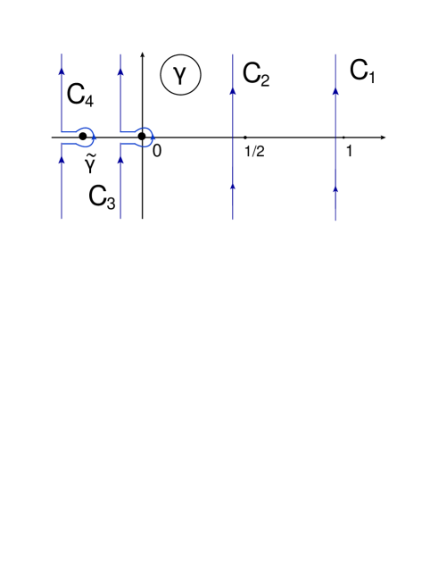
Figure 2: The contours of integration over $\gamma$

II.3 Vicinity of the saturation scale at $r^{2}\,Q^{2}_{s}\left(Y_{0},b\right)\,\approx\,1$

In this subsection we consider the kinematic region in which $N_{\rm el}\left(Y_{0},\boldsymbol{x}_{01},\boldsymbol{b}\right)$ is in the vicitity of the saturation scale $Q_{s}\left(Y_{0},b\right)$, but at $x^{2}_{01}\,Q^{2}_{s}\left(Y_{0},b\right)\,<\,1$. As it was found in Ref. IIML we have geometric scaling behaviour in this region, and the amplitude behaves as

$${N_{\rm el}\left(Y_{0},\boldsymbol{x}_{01},\boldsymbol{b}\right)\,\,\propto\,\,\left(x^{2}_{10}\,Q^{2}_{s}\left(Y_{0},b\right)\right)^{1-\gamma_{cr}}}$$ (17)

If $Y$ is close to $Y_{0}$, we can neglect the non-linear terms in Eq. (7), and we can solve the linear equation for $N^{D}$ with the initial condition of Eq. (8)

$${N^{D}\left(Y_{0},Y_{0};\boldsymbol{x}_{01},\boldsymbol{b}\right)\,\,=\,\,\mbox{c}^{2}\,\left(x^{2}_{10}\,Q^{2}_{s}\left(Y_{0},b\right)\right)^{2(1-\gamma_{cr})}};$$ (18)

II.3.1 Solution in the region where $N_{\rm el}\,\,<\,\,1$

Considering Eq. (18), one can see that in this kinematic region we can in general neglect the expression of Eq. (7) two terms: the term which is proportional to $\left(N^{D}\right)^{2}$ at $Y-Y_{0}\ll Y_{0}$, since it is of the order of $N^{4}_{\rm el}$, and the term which is proportional to $N^{D}N_{\rm el}\propto N^{3}_{\rm el}$, while we have to keep all other terms.

Therefore, the equation takes the form:

$$\frac{\partial N^{D}\left(Y,Y_{0};\boldsymbol{x}_{01},\boldsymbol{b}\right)}{\partial Y}\,=$$ (19)

$$\,\frac{\bar{\alpha}_{S}}{\pi}\int\,d^{2}\boldsymbol{x}_{2}\frac{{\mathbf{x^{2}_{01}}}}{{\mathbf{x^{2}_{02}}}\,{\mathbf{x^{2}_{12}}}}\Bigg{\{}\,N^{D}\left(Y,Y_{0};\boldsymbol{x}_{02},\boldsymbol{b}-\frac{1}{2}\boldsymbol{x}_{12}\right)+N^{D}\left(Y,Y_{0};\boldsymbol{x}_{12},\boldsymbol{b}-\frac{1}{2}\boldsymbol{x}_{02}\right)\,-\,N^{D}\left(Y,Y_{0};\boldsymbol{x}_{01},\boldsymbol{b}\right)$$

$$+2\,N_{\rm el}(Y;\boldsymbol{x}_{02},\boldsymbol{b}-\frac{1}{2}\boldsymbol{x}_{12})N_{\rm el}(Y;\boldsymbol{x}_{12},\boldsymbol{b}-\frac{1}{2}\boldsymbol{x}_{02})]\,\Bigg{\}}.$$

In this equation we take into account the corrections of the order $N^{2}_{el}$, but neglected the terms of the order of $N^{3}_{el}$ and $N^{4}_{el}$, assuming they are small. We believe that this equation will allow us to take into account the correction for $N_{el}\approx 0.4-0.5$,

Taking derivatives with respect to $Y_{0}$, we re-write Eq. (19) for the amplitude $n^{D}\left(Y,Y_{0},\boldsymbol{x}_{01},\boldsymbol{b}\right)$ that has been introduced in Eq. (9). It takes the form of the linear equation:

$$\frac{\partial n^{D}\left(Y,Y_{0};\boldsymbol{x}_{01},\boldsymbol{b}\right)}{\partial Y}\,=$$ (20)

$$\,\frac{\bar{\alpha}_{S}}{\pi}\int\,d^{2}\boldsymbol{x}_{2}\frac{{\mathbf{x^{2}_{01}}}}{{\mathbf{x^{2}_{02}}}\,{\mathbf{x^{2}_{12}}}}\Bigg{\{}\,n^{D}\left(Y,Y_{0};\boldsymbol{x}_{02},\boldsymbol{b}-\frac{1}{2}\boldsymbol{x}_{12}\right)+n^{D}\left(Y,Y_{0};\boldsymbol{x}_{12},\boldsymbol{b}-\frac{1}{2}\boldsymbol{x}_{02}\right)\,-\,n^{D}\left(Y,Y_{0};\boldsymbol{x}_{01},\boldsymbol{b}\right)\Bigg{\}}$$

The initial condition for this equation is the following:

$$n^{D}\left(Y=Y_{0},Y_{0};\boldsymbol{x}_{01},\boldsymbol{b}\right)\,\,=\,\,\frac{\partial}{\partial Y_{0}}N^{2}_{el}\left(Y_{0},\boldsymbol{x}_{01},\boldsymbol{b}\right)$$ (21)

The elastic amplitude has the form:

$$N_{\rm el}(Y;x_{10},b)\,\,=\,\,{\rm c}\left(x^{2}_{10}\,Q^{2}_{s}\left(Y,b\right)\right)^{\bar{\gamma}}\,\,\equiv\,\,{\rm c}\,\left(\frac{Q^{2}_{s}\left(Y_{0},b\right)}{Q^{2}_{0}}\right)^{\bar{\gamma}}\,e^{\bar{\gamma}\left(\bar{\alpha}_{S}\kappa\left(Y-Y_{0}\right)\,-\,\xi\right)}$$ (22)

where $\xi\,\equiv\,\ln\left(1/\left(x^{2}_{10}\,Q^{2}_{0}\right)\right)$.

Taking the double Mellin transform, and defining $\bar{Y}=\bar{\alpha}_{S}Y$

$${n^{D}\left(Y,Y_{0},\xi,b\right)\,\,=\,\,\,\int_{C_{1}}\frac{d\gamma d\omega}{(2\pi i)^{2}}\,\phi(\omega,\gamma)\,e^{\omega\left(\bar{Y}-\bar{Y}_{0}\right)\,\,+\,\,\left(\gamma-1\right)\xi}}$$ (23)

we obtain the solution to the equation of Eq. (20) in the following form:

$${n^{D}\left(Y,Y_{0},\xi,b\right)\,\,=\,\,\,\int_{C_{1}}\frac{d\gamma d\omega}{(2\pi i)^{2}}\,\frac{\phi_{in}\left(\gamma,Y_{0},\boldsymbol{b}^{\prime}\right)}{\omega-\chi\left(\gamma\right)}\,e^{\omega\left(\bar{Y}-\bar{Y}_{0}\right)\,\,+\,\,\left(\gamma-1\right)\xi}}$$ (24)

where $\phi_{in}$ has to be determined from the initial condition of Eq. (36), and it has the form

$$\phi_{in}\left(\gamma,Y_{0},\boldsymbol{b}^{\prime}\right)\,\,=\,\,2\bar{\gamma}\kappa\,\Big{(}\frac{Q^{2}_{s}\left(Y_{0},b^{\prime}\right)}{Q^{2}_{0}}\Big{)}^{2\bar{\gamma}}\,\frac{c^{2}}{\gamma-\tilde{\gamma}}$$ (25)

Therefore, the solution takes the form (see Fig. 1 for notations):

$${n^{D}\left(Y,Y_{0},\xi,b\right)\,\,=\,\,2\bar{\alpha}_{S}\,\bar{\gamma}\,\kappa\,c^{2}\Big{(}\frac{Q^{2}_{s}\left(Y_{0},b^{\prime}\right)}{Q^{2}_{0}}\Big{)}^{2\bar{\gamma}}\int_{C_{1}}\frac{d\gamma}{2\pi i}\,\frac{1}{\gamma-\tilde{\gamma}}\,e^{\chi\left(\gamma\right)\left(\bar{Y}-\bar{Y}_{0}\right)\,\,+\,\,\left(\gamma-1\right)\xi}}$$ (26)

with $\gamma_{cr}=0.37$ and $\bar{\gamma}\,=\,\,1-\gamma_{cr}=0.63$ ,$\tilde{\gamma}=-1+2\gamma_{cr}=-0.26$. $\chi\left(\gamma\right)$ is given by Eq. (II.2).

The choice of the contour of integration over $\gamma$ (see Fig. 2) is standard for the solution of the BFKL Pomeron, and correctly reproduces the calculation of the gluon emission in perturbative QCD.

The contour of integration ($C_{1}$) is shown in Fig. 2. Since $\xi>0$ we can safely move this contour, and for large values of $\delta Y=Y-Y_{0}$ and $\xi$, we can take the integral using the method of steepest decent. For $\alpha_{S}\delta Y\,\gg\,\xi$ we evaluate the integral by this method, integrating along the contour $C_{2}$ which crosses the real axis at $\gamma$ close to $\frac{1}{2}$. At $\xi\,\gg\,\bar{\alpha}_{S}\,\delta Y$, we can integrate by the same method, but moving contour $C_{2}$ closer to $y$-axis in Fig. 2. For $\delta Y=0$ we can close the counter over pole $\gamma=\bar{\gamma}$. However, for $\delta Y\sim 1$ we cannot use the same method, since at $\gamma=0$ we have singularities in the kernel $\chi(\gamma)$. We cannot use the method of steepest decent for such small values of $\delta Y$.

II.3.2 Solution in the saddle point approximation

Using solution of Eq. (26) we can find the saturation momentum for the process of diffraction production, calculating the integral over $\gamma$ by the method of steepest descent. $Q_{s}$ can be determined from the following two equations:

$$\bar{\alpha}_{S}\frac{d\chi\left(\gamma\right)}{d\gamma}\left(Y-Y_{0}\right)\,\,+\,\,\xi = \,\,0;$$ (27)

$$\bar{\alpha}_{S}\chi\left(\gamma\right)\left(Y-Y_{0}\right)\,\,+\,\,\left(\gamma-1\right)\xi = \,\,0;$$ (28)

Eq. (27) is the equation for the saddle point while Eq. (28) is the condition that the solution is a constant on the critical line $x^{2}_{10}=1/Q_{s}^{2}$. The solution of these two equation is well known $\gamma=\gamma_{cr}=0.37$ and $Q^{2}_{s}\left(Y\right)\,=\,Q^{2}\left(Y_{0}\right)\,\exp\left(\bar{\alpha}_{S}\kappa\left(Y-Y_{0}\right)\right)$ with $\kappa=\chi\left(\gamma_{cr}\right)/(1-\gamma_{cr})$. In the vicinity of the saturation scale Eq. (26) behaves as

$$\frac{2\,\bar{\alpha}_{S}\,\bar{\gamma}\,\kappa\,c^{2}}{\gamma_{cr}-\tilde{\gamma}}\,\left(\frac{Q^{2}\left(Y_{0},b^{\prime}\right)}{Q^{2}_{0}}\right)^{2\,\bar{\gamma}}\left(x^{2}_{10}\,Q^{2}_{s}\left(Y-Y_{0},\boldsymbol{b}-\boldsymbol{b}^{\prime}\right)\right)^{1-\gamma_{cr}}$$ (29)

One can see that there is no geometric scaling behavior of the scattering amplitude $n^{D}$, even at large $Y-Y_{0}$. We can also see that the solution does not satisfy the initial condition. It stems from Eq. (27) and Eq. (28), which both are correct only if $\delta Y\,\gg\,1$, assuming that the saddle point value of $\gamma$ is not close to $\tilde{\gamma}$. We need to re-write these equations to take into account the possibility that $\gamma_{SP}\to\tilde{\gamma}$ taking into account the factor $1/(\gamma-\tilde{\gamma})$. The equations for the saddle point take the form:

$$\bar{\alpha}_{S}\frac{d\chi\left(\gamma\right)}{d\gamma}\left(Y-Y_{0}\right)\,\,+\,\,\xi\,\,+\,\,\frac{1}{\gamma-\tilde{\gamma}} = \,\,0;$$ (30)

$$\bar{\alpha}_{S}\chi\left(\gamma\right)\left(Y-Y_{0}\right)\,\,+\,\,\left(\gamma-1\right)\xi\,-\,\ln\left(\gamma-\tilde{\gamma}\right) = \,\,0;$$ (31)

The contribution of the additional term is essential, only if $\gamma_{SP}\to\tilde{\gamma}$, but even $\gamma=0$ which corresponds the integration with the contour $C_{3}$ (see Fig. 2), is still not close to $\tilde{\gamma}$. Bearing this in mind, we prefer to treat $\delta Y\ll 1$ without using the method of steepest descent.

II.3.3 Solution for $\delta Y\ll 1$.

In this section we will return to the discussion of Eq. (26) at $\delta Y=Y-Y_{0}\,\leq\,1$. In this kinematic region, we cannot use the method of steepest descent, and have to look for a different approach. First, let us analyze the solution iterating the equation keeping $\delta Y\,\,\ll\,1$. To obtain the solution as a sum of $\left(\delta Y\right)^{n}$ contributions we need to expand

$$e^{\bar{\alpha}_{S}\chi\left(\gamma\right)\left(Y-Y_{0}\right)}\,\,=\,\,\sum^{\infty}_{n=0}\,\frac{\left(\bar{\alpha}_{S}\chi(\gamma)\,\delta Y\right)^{n}}{n!}\,\xrightarrow{\gamma\to 0}\,\sum^{\infty}_{n=0}\,\frac{1}{n!}\left(\frac{\bar{\alpha}_{S}\,\delta Y}{\gamma}\right)^{n}$$ (32)

For each term of this series, we need to plug in our solution and integrate it over $\gamma$. This integral takes the following form for the third term in Eq. (26) for $n\,\geq\,1$:

$$\oint_{C_{3}}\,d\gamma\,\left(\frac{\bar{\alpha}_{S}\,\delta Y}{\gamma}\right)^{n}\frac{e^{\left(\gamma-1\right)\xi}}{\gamma-\tilde{\gamma}}\,\,=\,\,\left(\bar{\alpha}_{S}\,\delta Y\right)^{n}\Bigg{\{}\frac{1}{\tilde{\gamma}}\frac{1}{(n-1)!}\left(\frac{e^{\left(\gamma-1\right)\xi}}{\gamma-\tilde{\gamma}}\right)^{(n)}_{\gamma,\gamma\to 0}\,+\,\frac{1}{\tilde{\gamma}^{n}}\,e^{\left(\tilde{\gamma}-1\right)\xi}\Bigg{\}}$$ (33)

For $n=0$, we have the contribution only of the second term in Eq. (33).

In Eq. (32) we evaluated the integral, closing the contour over the singularities of the BFKL kernel, which is the pole at $\gamma=0$, and over the pole $\gamma=\tilde{\gamma}$. The BFKL kernel also has poles at $\gamma\,=\,-n,\,n=1,2,3\dots$, but their contributions are exponentially suppressed with $\xi$ leading to the next twists contributions. Eq. (33) can be re-written as follows

$$\oint_{C_{3}}\,d\gamma\,\left(\frac{\bar{\alpha}_{S}\,\delta Y}{\gamma}\right)^{n}\frac{e^{\left(\gamma-1\right)\xi}}{\gamma-\tilde{\gamma}}\,\,=\,\,\left(\frac{\bar{\alpha}_{S}\,\delta Y}{\tilde{\gamma}}\right)^{n}\,e^{-\xi}\,\Bigg{\{}\frac{1}{\tilde{\gamma}}\frac{1}{(n-1)!}\,\sum_{k=0}^{n-1}\frac{\left(\tilde{\gamma}\,\xi\right)^{k}}{k!}\,\,+\,\,e^{\tilde{\gamma}\,\xi}\Bigg{\}}$$ (34)

The last term in Eq. (34) is the contribution at the pole $\gamma=\tilde{\gamma}$, while the first term is the sum of logs term giving the leading twist perturbative series.

Bearing this in mind we can re-write Eq. (26) in the following form

$$n^{D}\left(Y,Y_{0},\xi,b\right)\,\,=\\ \,\,2\bar{\alpha}_{S}\bar{\gamma}\,\kappa\,\,c^{2}\,\left(\frac{Q^{2}\left(Y_{0},b^{\prime}\right)}{Q^{2}_{0}}\right)^{2\bar{\gamma}}\Bigg{\{}\int_{C_{1}-C_{4}}\frac{d\gamma}{2\pi i}\,\frac{1}{\gamma-\tilde{\gamma}}\,e^{\chi\left(\gamma\right)\left(\bar{Y}-\bar{Y}_{0}\right)\,\,+\,\,\left(\gamma-1\right)\xi}\,\,+\,\,e^{\left(\tilde{\gamma}-1\right)\xi}\,e^{\bar{\alpha}_{S}\chi\left(\tilde{\gamma}\right)\,\left(Y-Y_{0}\right)}\Bigg{\}}$$ (35)

The first term in Eq. (35) is the difference between two integrals with contour $C_{1}$ and $C_{4}$, while the last term is the result of integrating over $\gamma$, with the contour $C_{4}$. The advantage of this form for the equation, is that it satisfies the initial condition, since the first term is equal to zero at $\delta Y=0$, and the first term generates all perturbative logs with respect to the dipole sizes.

In the situation when $\bar{\alpha}_{S}\xi\,\gg\,1$ while $\bar{\alpha}_{S}\,\ll\,1$ the first term reduces to the double log approximation generating the contribution

$$n^{D}_{\rm 1-st\,term\,of\,{Eq.~{}(\ref{CR2})}}\left(Y,Y_{0},r\right)\,\,=$$ (36)

$$2\bar{\alpha}_{S}\bar{\gamma}\,\kappa\,c^{2}\,\left(\frac{Q^{2}\left(Y_{0},b^{\prime}\right)}{Q^{2}_{0}}\right)^{2\bar{\gamma}}\frac{\bar{\alpha}_{S}\delta Y}{\bar{\gamma}}\,e^{-\xi}\,\sum^{\infty}_{n=1}\frac{1}{n!(n-1)!}\left(\bar{\alpha}_{S}\delta Y\xi\right)^{n-1}\,=\,2c^{2}\,\left(\frac{Q^{2}\left(Y_{0},b^{\prime}\right)}{Q^{2}_{0}}\right)^{2\bar{\gamma}}\frac{1}{\bar{\gamma}}\frac{1}{2}\sqrt{\frac{\bar{\alpha}_{S}\delta Y}{\xi}}\,e^{-\xi}I_{1}\left(2\sqrt{\bar{\alpha}_{S}\delta Y\,\xi}\right)\,$$

which stems from the term with $\xi^{n-1}$ in Eq. (34).

Finally the double log contribution takes the form:

$$n^{D}\left(Y,Y_{0},r\right)\,\,=$$ (37)

$$\,2\bar{\alpha}_{S}\,\bar{\gamma}\,\kappa\,c^{2}\,\left(\frac{Q^{2}\left(Y_{0},b\right)}{Q^{2}_{s}\left(Y_{\rm in}\right)}\right)^{2\bar{\gamma}}\frac{1}{\bar{\gamma}}\Bigg{\{}\frac{1}{2}\sqrt{\frac{\bar{\alpha}_{S}\delta Y}{\xi}}\,e^{-\xi}I_{1}\left(2\sqrt{\bar{\alpha}_{S}\delta Y\,\xi}\right)\,+\,\,e^{\left(\tilde{\gamma}-1\right)\xi}\,e^{\bar{\alpha}_{S}\chi\left(\tilde{\gamma}\right)\,\left(Y-Y_{0}\right)}\Bigg{\}}$$

In appendix A we remove the assumption that $\bar{\alpha}_{S}\xi\gg\,1$.

II.3.4 Solution in the region where $N_{\rm el}\,\sim\,1$

In this kinematic region we need to keep the term which is proportional to $N_{el}\,N^{D}$ in Eq. (6) and solve the equation which takes the form

$$\frac{\partial n^{D}\left(Y,Y_{0};\boldsymbol{x}_{01},\boldsymbol{b}\right)}{\partial Y}\,=$$ (38)

$$\,\frac{\bar{\alpha}_{S}}{\pi}\int\,d^{2}\boldsymbol{x}_{2}\frac{{\mathbf{x^{2}_{01}}}}{{\mathbf{x^{2}_{02}}}\,{\mathbf{x^{2}_{12}}}}\Bigg{\{}\,n^{D}\left(Y,Y_{0};\boldsymbol{x}_{02},\boldsymbol{b}-\frac{1}{2}\boldsymbol{x}_{12}\right)+n^{D}\left(Y,Y_{0};\boldsymbol{x}_{12},\boldsymbol{b}-\frac{1}{2}\boldsymbol{x}_{02}\right)\,-\,n^{D}\left(Y,Y_{0};\boldsymbol{x}_{01},\boldsymbol{b}\right)$$

$$-\,4\,n^{D}(Y,Y_{0};\boldsymbol{x}_{02},\boldsymbol{b}-\frac{1}{2}\boldsymbol{x}_{12})\,\,N_{\rm el}(Y;\boldsymbol{x}_{12},\boldsymbol{b}-\frac{1}{2}\boldsymbol{x}_{02})\,\Bigg{\}}.$$

Therefore, we took into account terms $n^{D}\,N_{el}$ in comparison with the previous sections. We consider that $n^{D}\,N^{D}$ are sufficiently small, so that we can neglect the contributions $n^{D}\,N^{D}\,\sim N^{4}_{el}\,\ll 1$.

This equation looks simpler in the momentum representation:

$$N\left(x_{10},b,Y\right)\,\,\equiv\,\,x^{2}_{10}\int d^{2}\,k_{T}e^{i\boldsymbol{k}_{T}\cdot\boldsymbol{x}_{10}}N\left(k_{T},b,Y\right)$$ (39)

In the momentum representation Eq. (7) takes the form:

$$\frac{\partial n^{D}\left(Y,Y_{0};\boldsymbol{k}_{T},\boldsymbol{b}\right)}{\partial Y}\,=$$ (40)

$$\,\frac{\bar{\alpha}_{S}}{\pi}\int\,d^{2}\boldsymbol{k}^{\prime}_{T}\frac{1}{\left(\boldsymbol{k}^{\prime}_{T}-\boldsymbol{k}_{T}\right)^{2}}\Bigg{\{}\,n^{D}\left(Y,Y_{0};\boldsymbol{k^{\prime}}_{T},\boldsymbol{b}\right)-\,\frac{k^{2}_{T}}{\left(\boldsymbol{k}^{\prime}_{T}-\boldsymbol{k}_{T}\right)^{2}+k^{\prime 2}_{T}}\,n^{D}\left(Y,Y_{0};\boldsymbol{k}_{T},\boldsymbol{b}\right)\Bigg{\}}\,$$

$$\,+\,\bar{\alpha}_{S}\,2n^{D}\left(Y,Y_{0};\boldsymbol{k}_{T},\boldsymbol{b}\right)N^{D}\left(Y,Y_{0};\boldsymbol{k}_{T},\boldsymbol{b}\right)\,\,-\bar{\alpha}_{S}\,\,4\,n^{D}(Y,Y_{0};\boldsymbol{k}_{T},\boldsymbol{b})N_{\rm el}(Y;\boldsymbol{k}_{T},\boldsymbol{b})\,$$

We solve this equation using the semi-classical approach. In this approach we are looking for the solution in the form

$$n^{D}\left(Y,Y_{0};k_{T},b\right)\,\,\equiv\,\,n^{D}\left(Y,Y_{0};\rho=\ln\left(k^{2}_{T}/Q^{2}_{0}\right),b\right)\,=\,e^{S\left(Y,Y_{0},\rho,b\right)}$$ (41)

with

$$\,\,\,S\,=\,\omega\left(Y,Y_{0},\rho,b\right)\left(Y-Y_{0}\right)\,-\,\left(1-\gamma\left(Y,Y_{0},\rho,b\right)\right)\,\rho$$ (42)

where

$$\frac{\partial S\left(Y,Y_{0},\rho,b\right)}{\partial Y}\,\,=\,\,\omega\left(Y,Y_{0},\rho,b\right);~{}~{}~{}~{}~{}~{}~{}~{}~{}~{}~{}~{}~{}\frac{\partial S\left(Y,Y_{0},\rho,b\right)}{\partial\rho}\,\,=\,\,\gamma\left(Y,Y_{0},\rho,b\right)-1;$$ (43)

are smooth functions of $Y$ and $\rho$, and the following conditions are assumed:

$$\frac{\partial\,\omega(Y,Y_{0},\rho,b)}{\partial Y}\hskip 8.5359pt\ll\hskip 8.5359pt\omega^{2}(Y,Y_{0},\rho,b);\,\,\,\,\frac{\partial\,\omega(Y,Y_{0},\rho,b)}{\partial\rho}\hskip 8.5359pt\ll\hskip 8.5359pt\omega(Y,Y_{0},\rho,b)\,\left(1-\gamma(Y,Y_{0},\rho,b\right);\,\,\,$$ (44)

$$\frac{\partial\,\gamma(Y,Y_{0},\rho,b)}{\partial\rho}\hskip 8.5359pt\ll\hskip 8.5359pt\left(1-\gamma(Y,Y_{0},\rho,b)\right)^{2};\,\,\,\,\,\frac{\partial\,\gamma(Y,Y_{0},\rho,b)}{\partial Y}\hskip 8.5359pt\ll\hskip 8.5359pt\omega(Y,Y_{0},\rho,b)\,\left(1-\gamma(Y,Y_{0},\rho,b)\right);$$ (45)

Plugging Eq. (41) and Eq. (42) in Eq. (36) we have

$$\omega\left(Y,Y_{0},\rho,b\right)\,\,=\,\,\bar{\alpha}_{S}\,\left(\chi\left(\gamma\left(Y,Y_{0},\rho,b\right)\right)\,\,-\,\,4N_{\rm el}(Y;\rho,b)\right)\,\,$$ (46)

For the equation in the form

$$F(Y,\rho,S,\gamma,\omega)=0$$ (47)

where $S$ is given by Eq. (42), we can introduce the set of characteristic lines on which $\rho(t),Y(t),S(t),$ $\omega(t),$ and $\gamma(t)$ are functions of the variable $t$ (which we call artificial time), that satisfy the following equations:

$$(1.)\,\,\,\,\,\,\,\frac{d\rho}{d\,t}\,\,=\,\,F_{\gamma}\,\,=\,-\,\bar{\alpha}_{S}\,\frac{d\chi(\gamma)}{d\gamma}$$

$$(2.)\,\,\,\,\,\,\,\frac{d\,Y}{d\,t}\,\,=\,\,F_{\omega}\,\,=\,\,1\,\,\,\,\,\,\,$$ (48)

$$(3.)\,\,\,\,\,\,\,\frac{d\,\tilde{S}}{d\,t}\,\,=\,\,(\gamma\,-\,1)\,F_{\gamma}\,+\,\omega\,F_{\omega}\,\,=\,\,\bar{\alpha}_{S}\,\left(1\,-\,\gamma\right)\,\frac{d\chi(\gamma)}{d\gamma}\,\,+\,\,\omega$$

$$(4.)\,\,\,\,\,\,\,\frac{d\,\gamma}{d\,t}\,\,=\,\,-(\,F_{\rho}\,+\,(\gamma\,-\,1)\,F_{S}\,)\,\,=\,\,4\bar{\alpha}_{S}(1-\gamma_{cr})\,N_{\rm el}(Y;\rho,b)$$

$$(5.)\,\,\,\,\,\,\,\frac{d\,\omega}{d\,t}\,\,=\,\,-\,(\,F_{Y}\,+\,\omega\,F_{S}\,)\,\,=-\,\,4\bar{\alpha}_{S}^{2}\kappa\bar{\gamma}\,N_{\rm el}(Y;\rho,b)\,$$

In Eq. (48) we consider that

$$N^{2}_{\rm el}(Y;\rho,b)\,\,=\,\,{\rm c}\left(\frac{Q^{2}_{s}\left(Y,b\right)}{k^{2}_{T}}\right)^{\bar{\gamma}}\,\,\equiv\,\,{\rm c}\,\left(\frac{Q^{2}\left(Y_{0},b\right)}{Q^{2}_{0}}\right)^{\bar{\gamma}}\,e^{\bar{\gamma}\left(\bar{\alpha}_{S}\kappa\left(Y-Y_{0}\right)\,-\,\rho\right)}$$ (49)

with $\kappa=\chi\left(\gamma_{cr}\right)/(1-\gamma_{cr})$.

In Fig. 3 we plotted the numerical solutions of Eq. (48). One can see that the solution gives $\gamma\left(Y\right)$, which approach a constant at large $Y-Y_{0}$. This feature stem from Eq. (48)-4 since $N_{el}\to 0$ at large $\rho$.

Bearing this in mind one can see that Eq. (46) and Eq. (48) degenerate to Eq. (19) in the semiclassical approach, at large $Y$. Indeed, Fig. 4 shows that the solution to Eq. (19) shown in dashed lines in Fig. 4, is close to the solution of Eq. (47) for $Y\geq 2$.

Therefore, we need to consider the solution of Eq. (26) in the entire kinematic region where we can neglect the term proportional to $\left(N^{D}\right)^{2}$ in Eq. (7).

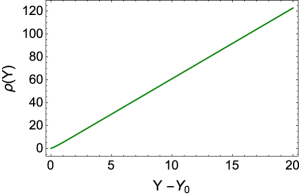
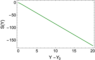
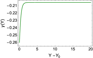
Fig. 3-a	Fig. 3-b	Fig. 3-c

Figure 3: The numerical solution to Eq. (48). Constant ${\rm c}$ in Eq. (39) is chosen ${\rm c}$=0.05 in accord with the description of the HERA data in Ref.CLP . $\alpha_{S}=0.25$. $\chi\left(\gamma\right)=2\psi(1)-\psi(\gamma)-\psi(1-\gamma)$, where $\psi(z)=d\ln\Gamma(z)/dz$ and $\Gamma$ is Euler gamma-function. $N_{\rm el}\left(Y_{0},\rho\right)={\rm c}\left(Q^{2}_{s}\left(Y_{0}\right)/k^{2}_{T}\right)^{\bar{\gamma}}$.

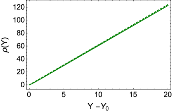
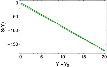
Fig. 4-a	Fig. 4-b

Figure 4: The comparison of the numerical solution to Eq. (48) and to Eq. (19) in semi-classical approximation. The solid lines denote the solution to Eq. (48) shown in Fig. 3, while the dashed lines describe the solution to Eq. (19) in the semi-classical approximation. For $\xi$ at $Y=0$ we use $\xi$= 0 in the solution to Eq. (48) and $\xi$=3 in the solution to Eq. (19). Constant ${\rm c}$ in Eq. (39) is chosen ${\rm c}$=0.05. $\alpha_{S}=0.25$. $\chi\left(\gamma\right)=2\psi(1)-\psi(\gamma)-\psi(1-\gamma)$, where $\psi(z)=d\ln\Gamma(z)/dz$ and $\Gamma$ is Euler gamma-function. $N_{\rm el}\left(Y_{0},\rho\right)={\rm c}\left(Q^{2}_{s}\left(Y_{0}\right)/k^{2}_{T}\right)^{\bar{\gamma}}$.

II.4 Solution in the region where $N_{\rm el}\,\ll\,1$

In this section we consider the solution, in the region where $N_{\rm el}\left(Y_{0},x_{01},b\right)$ is a solution to the linear BFKL equation, which has the following general form

$$N_{\rm el}\left(Y_{0},x_{01},b\right)\,\,=\,\,\int^{\epsilon+i\infty}_{\epsilon+i\infty}\frac{d\gamma}{2\,\pi\,i}\,n_{\rm in}\left(\gamma,b\right)\,e^{\chi\left(\gamma\right)\,Y_{0}\,+\,\left(\gamma-1\right)\xi}$$ (50)

where $n_{\rm in}\left(\gamma,b\right)$ should be found from the initial condition at $Y_{0}=0$. Recall, that $Y_{0}\equiv\bar{\alpha}_{S}Y_{0}$, as we have discussed above and $\xi=\ln\left(1/(x^{2}_{10}Q^{2}_{0}\right)$. In the region of large $Y_{0}$, we take only the leading term in $\chi\left(\gamma\right)\xrightarrow{\gamma\ll 1}1/\gamma$ into account, and take the integral by the method of steepest descent. As the result we obtain a solution in the double log approximation (DLA) of perturbative QCD. At large $Y_{0}$ we can re-write $N^{2}_{\rm el}\left(Y_{0},x_{01},b\right)$ in the form

$$N^{2}_{\rm el}\left(Y_{0},x_{01},b\right)\,\, = \,\,\int^{\epsilon+i\infty}_{\epsilon+i\infty}\frac{d\gamma d\gamma^{\prime}}{(2\,\pi\,i)^{2}}\,n_{\rm in}\left(\gamma-\gamma^{\prime},b\right)\,n_{\rm in}\left(\gamma^{\prime},b\right)\,e^{\left(\chi\left(\gamma-\gamma^{\prime}\right)\,+\,\chi\left(\gamma^{\prime}\right)\right)\,Y_{0}\,+\,\left(\gamma-2\right)\xi}$$

$$\mbox{MOSD for integration over~{}~{}}\gamma^{\prime} \,=\, \,\,\int^{\epsilon+i\infty}_{\epsilon+i\infty}\frac{d\gamma}{2\,\pi\,i}\,n^{2}_{\rm in}\left(\gamma/2,b\right)\,e^{2\chi\left(\gamma/2\right)\,Y_{0}\,+\,\left(\gamma-2\right)\xi}$$ (51)

where MOSD means the method of steepest descent.

Bearing Eq. (II.4) in mind, we obtain the solution to the BFKL equation for $N^{D}$ in the form

$$n^{D}\,\left(Y,Y_{0},\xi,b\right)\,\,=\,\,\int^{\epsilon+i\infty}_{\epsilon+i\infty}\frac{d\gamma}{2\,\pi\,i}\,n^{D}\left(Y_{0},\gamma\right)\,e^{\chi\left(\gamma\right)\left(Y-Y_{0}\right)\,+\,\left(\gamma-1\right)\xi}$$ (52)

Calculating $n^{D}\left(Y_{0},\gamma\right)$ from Eq. (II.4) we obtain

$$n^{D}\,\left(Y,Y_{0},\xi,b\right)\,\,=\,\,\,=\,\int^{\epsilon+i\infty}_{\epsilon+i\infty}\frac{d\gamma}{2\,\pi\,i}\,n^{2}_{\rm in}\left(\frac{\gamma+1}{2},b\right)\,e^{2\chi\left(\frac{1}{2}(\gamma+1)\right)\,Y_{0}+\chi\left(\gamma\right)\left(Y-Y_{0}\right)\,+\,\left(\gamma-1\right)\xi}$$ (53)

Taking the integral over $\gamma$ in the DLA, the equation for the saddle point takes the form

$$\xi\,\,=\,\,\frac{Y-Y_{0}}{\gamma^{2}_{\rm SP}}\,\,+\,\,\frac{4\,Y_{0}}{\left(\gamma_{\rm SP}+1\right)^{2}},$$ (54)

Eq. (54) has four solutions (see Fig. 5). Two of them have imaginary parts while other two are real. At $Y-Y_{0}\,\ll\,\xi-4Y_{0}$ and $\gamma_{\rm SP}\to\sqrt{\frac{Y-Y_{0}}{\xi\,-\,4\,Y_{0}}}$. At $Y-Y_{0}\,\ll\,Y_{0}\,\ll\,\xi$ one can find: $\gamma_{\rm SP}\,\,\to\,\,-1\,+\,\sqrt{\frac{4Y_{0}}{\xi-(Y-Y_{0})}}$. In this limit we see that our solution satisfies the initial conditions in the DLA.

For large $Y-Y_{0}$ the solution has then form

$$N^{D}_{\rm DLA}\left(Y,Y_{0},\xi,b\right)\,\,=\,\,\sqrt{\frac{\pi(Y-Y_{0})}{\xi^{3}}}\,n^{2}_{\rm in}\left(\gamma_{SP}=\frac{1}{2}\sqrt{\frac{Y-Y_{0}}{\xi}},b\right)\,e^{2\sqrt{\left(Y-Y_{0}\right)\xi}\,\,-\,\,\,\xi}$$ (55)

From Eq. (55) one can see that the solution reaches the saturation bound at

$$\xi_{\rm sat}\,=\,4\left(Y-Y_{0}\right)\,~{}~{}~{}~{}~{}~{}~{}~{}~{}~{}~{}Q^{2}_{s}\left(Y,Y_{0}\right)\,=\,Q^{2}_{0}\,e^{\left(Y-Y_{0}\right)}\,\,=\,\,Q^{2}_{s}\left(Y-Y_{0}\right)$$ (56)

and behaves in the vicinity of this bound as

$$n^{D}_{\rm DLA}\left(Y,Y_{0},\xi,b\right)\,\,\propto\,\,\left(x^{2}_{10}\,Q^{2}_{s}\left(Y-Y_{0}\right)\right)^{\frac{1}{2}}$$ (57)

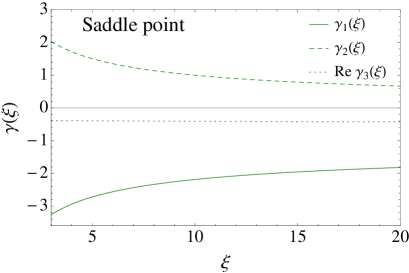
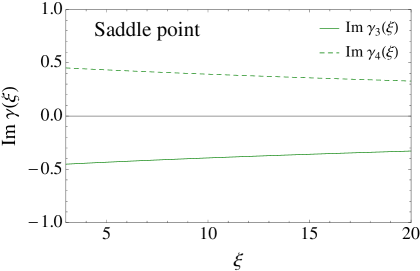
Fig. 5-a		Fig. 5-b

Figure 5: $\gamma_{\rm SP}\left(\xi,Y,Y_{0}\right)$ versus $\xi$ at $Y_{0}$ = 3, $Y$=10.

III The model

As we have discussed, the main idea of building the saturation model has been formulated in Ref.IIM : it is the matching of two analytical solutions in the vicinity of the saturation scale, and deep inside of the saturation domain.

III.1 The input: $N_{el}\left(r,Y\right)$ in our saturation model

As we have mentioned, the initial condition for the equation for $N^{D}$ (see Eq. (8)) is determined by $N_{el}$, which we have found from the HERA data for the deep inelastic structure function in Ref.CLP . For completeness of presentation we describe the main formulae of this model which illustrates our procedure for the model building.

In the vicinity of the saturation scale or, in other words, for the dipole size $r$ in the region: $\tau\,\equiv\,r^{2}\,Q^{2}_{s}\left(Y_{0},b\right)\,\,\to\,\,1$ we use the CGC formula for $N_{el}\left(r,Y_{0}\right)$KOLEB ; IIML ; MUT

$$N^{\tau\to 1}_{el}\left(r,Y_{0}\right)\,\,=\,\,N_{0}\,\left(r^{2}\,\,Q^{2}_{s}\left(Y_{0}\right)\right)^{1-\gamma_{cr}}$$ (58)

where $N_{0}$ is the phenomenological parameter that has been found in Ref.CLP .

$Q_{s}$ is the saturation momentum which we will discuss below. The values of $\gamma_{cr}$ can be found from the following equation:

$$\frac{\chi\left(\gamma_{cr}\right)}{1-\gamma_{cr}}\,\,=\,\Big{|}\frac{d\chi\left(\gamma_{cr}\right)}{d\gamma_{cr}}\Big{|}$$ (59)

In Eq. (59) $\chi\left(\gamma\right)$ is the BFKL kernel that takes the form

$$\chi\left(\gamma\right)\,=\,2\,\psi\left(1\right)\,-\,\psi\left(\gamma\right)\,-\,\psi\left(1-\gamma\right)$$ (60)

where $\psi\left(z\right)$ is the digamma function.

Deep inside of the saturation domain, where $\tau\,\equiv\,r^{2}\,Q^{2}_{s}\left(Y,b\right)\,\gg\,1$, we use the analytical solution to the non-linear equation given in Ref.LETU

$$N^{\tau\gg 1}_{el}\left(r,Y_{0}\right)\,\,=\,1\,\,-\,\,2\,A\,\exp\left(-\frac{z^{2}}{2\,\lambda}\right)$$ (61)

where

$$z\,\,=\,\,\ln\left(r^{2}\,Q^{2}_{s}\left(Y,b\right)\right)\,\,=\,\,\ln\left(r^{2}Q^{2}\left(Y=Y_{in},b\right)\right)\,\,+\,\,\lambda\left(Y-Y_{in}\right)\,\,=\,\,\xi\,\,+\,\,\lambda\,\left(Y-Y_{0}\right)$$ (62)

where $\xi$ and $\lambda$ are related to the behaviour of the saturation scale

$$Q^{2}_{s}\left(Y_{0},b\right)\,\,=\,\,Q^{2}\left(Y=Y_{in},b\right)e^{\lambda\,\left(Y_{0}-Y_{in}\right)}\,\,=\,\,Q^{2}\left(Y=Y_{in},b\right)\left(\frac{x_{in}}{x}\right)^{\lambda}$$ (63)

where $Y_{in}=\ln(1/x_{in})$ shows the initial value of $x$ from which we start low $x$ evolution. This is a phenomenological parameter of the model. The phenomenological dependence on $b$ of the initial saturation scale $Q^{2}\left(Y=Y_{in},b\right)$ we have discussed in the introduction (see Eq. (1)). Finally, we use the following $Q^{2}\left(Y=Y_{in},b\right)$

$$Q^{2}\left(Y=Y_{in},b\right)\,\,=\,\,Q^{2}_{0}\,S\left(b\right)\,\,=\,\,Q^{2}_{0}\,\left(m\,b\,K_{1}\left(m\,b\right)\right)^{\frac{1}{1-\gamma_{cr}}}$$ (64)

Using Eq. (II.2)-Eq. (64) one can see that $\xi\,=\,\,\ln\left(r^{2}\,Q^{2}\left(Y_{in};b\right)\right)$ in Eq. (II.2). The value of $\lambda$ can be calculated and it is equal to $\lambda\,=\,\bar{\alpha}_{S}\,\chi\left(\gamma_{cr}\right)/(1-\gamma_{cr})$. However, in describing the experimental data in Ref.CLP , we consider $\lambda$ as the independent fitting parameter, since the next-to-leading correction turns out to be large.

Parameter $A$ in Eq. (61) should be found from the matching procedure of two solution at $z=z_{m}$:

$$N^{\tau\to 1}\left(z=z_{m}\right)\,=\,N^{\tau\gg 1}\left(z=z_{m}\right);~{}~{}~{}~{}~{}~{}~{}~{}~{}~{}~{}\frac{dN^{\tau\,\to\,1}\left(z=z_{m}\right)}{dz_{m}}\,=\,\frac{dN^{\tau\gg 1}\left(z=z_{m}\right)}{dz_{m}};$$ (65)

However, it turns out that Eq. (61) cannot satisfy Eq. (65). In Ref.CLM the correction to Eq. (61) has been found. The amplitude of Eq. (61) with the corrections takes the form:

$$N^{\tau\,\gg\,1}\left(z\right) \,=\, 1-2\,Ae^{-{\cal Z}}\,\,-\,\sqrt{2\lambda}\,A^{2}\,\frac{1}{\sqrt{{\cal Z}}}e^{-2{\cal Z}}\,\,+\,\,{\cal O}\left(e^{-3{\cal Z}}\right)$$ (66)

$${\cal Z} = \frac{\left(z-\frac{1}{2}A\sqrt{\lambda\pi/2}-2\psi(1)\right)^{2}}{2\lambda}$$

which has been used in the Eq. (65).

It should be stressed that all phenomenological parameters for the elastic amplitude has been extracted from the experimental data for $F_{2}$ at HERA (see Table 1).

$\lambda$	$N_{0}$	m ($GeV$)	$Q^{2}_{0}$ ($GeV^{2}$)	$m_{u}$(MeV)	$m_{d}$(MeV)	$m_{s}$(MeV)	$m_{c}$(GeV)	$\chi^{2}/d.o.f.$
0.197	0.34	0.75	0.145	2.3	4.8	95	1.4	178/155 =1.15
0.184	0.46	0.75	0.118	140	140	140	1.4	176/154 = 1.14

Table 1: Parameters of the model which has been extracted from DIS experiment in Ref.CLP . $\lambda$, $N_{0}$, $m$ and $Q^{2}_{0}$ ($Q^{2}_{0}\,=\,m^{2}\,x^{\lambda}_{in}$) are fitted parameters. The masses of quarks are not considered as fitted parameters and two sets of parameters, that are shown in the table, relate to two choices of the quark masses: the current masses and the masses of light quarks are equal to $140\,MeV$ which is the typical infra-red cutoff in our approach.

III.2 $N^{D}\left(r,Y,Y_{0}\right)$ in the model: matching procedure

III.2.1 $\tau_{0}\,=\,r^{2}\,Q^{2}_{s}\left(Y_{0},b^{\prime}\right)\,\to\,1$

In the kinematic region where $\tau_{0}\,=\,r^{2}\,Q^{2}_{s}\left(Y_{0},b^{\prime}\right)\,\to\,1$ , $\tau\,=\,r^{2}\,Q^{2}_{s}\left(Y,b\right)\,\to\,1$ and $\tau_{D}\,=\,r^{2}\,Q^{2}_{s}\left(Y-Y_{0},\boldsymbol{b}-\boldsymbol{b}^{\prime}\right)\,\leq\,1$ we suggest to use Eq. (37) which we re-write as follows

$$n^{D}_{\tau_{0}\to 1,\tau\to 1,\tau_{D}\leq 1}\left(Y,Y_{0},\xi,b\right)\,\,=$$ (67)

$$\,\,2\bar{\gamma}\,\lambda\,\Bigg{\{}\Bigg{(}\int d^{2}b^{\prime}\,\left(\frac{Q^{2}_{s}\left(Y_{0},b^{\prime}\right)}{Q^{2}_{0}}\right)^{2\bar{\gamma}}N_{1}\,\left(Y-Y_{0}\right)\left(r^{2}\,Q^{2}_{s}\left(Y-Y_{0},\boldsymbol{b}-\boldsymbol{b}^{\prime}\right)\right)^{\bar{\gamma}}\Bigg{)}\,\,+\,\,e^{-\lambda_{1}\left(Y-Y_{0}\right)}N^{2}_{el}\left(Y,r,b\right)\Bigg{\}}$$

The first term in Eq. (67) corresponds to the first term in Eq. (37), which we simplify taking into account the experience in the description of the elastic amplitude (see IIM ; SATMOD0 ; SATMOD1 ; BKL ; SATMOD2 ; SATMOD3 ; SATMOD4 ; SATMOD5 ; SATMOD6 ; SATMOD7 ; SATMOD8 ; SATMOD9 ; SATMOD10 ; SATMOD11 ; SATMOD12 ; SATMOD13 ; SATMOD14 ; SATMOD15 ; SATMOD16 ; SATMOD17 ; CLP ; CLP1 ). It was shown in these papers that we can describe the solution to the evolution equation taking the amplitude in the form of Eq. (58) replacing $1-\gamma_{cr}$ in Eq. (58) and in Eq. (67) by the following expression

$$1\,-\,\gamma_{cr}\,\,\to\,\,1\,-\,\gamma_{cr}\,\,-\,\,\frac{1}{2\,\kappa\,\lambda\,Y}\,\ln\ \left(r^{2}\,Q^{2}_{s}\left(b\right)\right)$$ (68)

where $\lambda=\bar{\alpha}_{S}\left(\chi\left(\gamma_{cr}\right)/\left(1-\gamma_{cr}\right)\right)$ and $\kappa\,=\,\chi^{\prime\prime}\left(\gamma_{cr}\right)/\chi^{\prime}\left(\gamma_{cr}\right)$. The factor $Y-Y_{0}$ is introduced to reflect the general features of the first term in Eq. (37) which is proportional to this factor. The saturation momentum $Q_{s}\left(Y-Y_{0},\boldsymbol{b}-\boldsymbol{b}^{\prime}\right)$ in QCD has the general form

$$Q^{2}_{s}\left(Y-Y_{0},\boldsymbol{b}-\boldsymbol{b}^{\prime}\right)\,\,=\,\,Q^{2}_{s}\left(Y_{0},b^{\prime}\right)\,e^{\kappa\,\left(Y-Y_{0}\right)}$$ (69)

where $Q_{s}\left(Y_{0},b^{\prime}\right)$ is the initial transverse momentum at $Y=Y_{0}$. However, as we have discussed above, we introduce the non-perturbative corrections in the behaviour at large impact parameter in the $b$-dependence of the saturation scale. Bearing this in mind we use the following parameterization of $Q_{s}\left(Y-Y_{0},\boldsymbol{b}-\boldsymbol{b}^{\prime}\right)$

$$Q^{2}_{s}\left(Y-Y_{0},\boldsymbol{b}-\boldsymbol{b}^{\prime},\boldsymbol{b}^{\prime}\right)\,\,=\,\,Q^{2}_{0}\,S\left(\boldsymbol{b}^{\prime}\right)\,e^{-m_{1}\,|\boldsymbol{b}-\boldsymbol{b}^{\prime}|}\,e^{\lambda\,Y}$$ (70)

where parameters $Q_{0}$, $\lambda$ and mass $m$ in $S\left(b\right)$ (see Eq. (64)) have been determined in our previous paper CLP from the fit of the elastic data. The parameter $m_{1}$ has to be extracted from the fit of the diffraction production as well as parameters $N_{1}$ and $\lambda_{1}$. In the leading order of perturbative QCD $\lambda_{1}=\chi\left(\tilde{\gamma}\right)$, but as well as for the energy behaviour of the saturation momentum, the higher order corrections are large, and we view these two parameters: $\lambda$ and $\lambda_{1}$ as the phenomenological parameters which we have to extract from the experimental data.

We need to use the matching procedure analogous to Eq. (65) for $n^{D}\,=\,-\,d{\cal N}^{D}dY_{0}$ using Eq. (15) in the form

$${{\cal N}^{D}_{\tau_{0}\to 1,\tau\gg 1}(Y,Y_{0};r)\,\,=\,\,1\,-\,G\left(\tau_{0}\,=\,r^{2}\,Q^{2}_{s}\left(Y_{0};b\right),Y_{0}\right)\,\,e^{-z^{2}/2\kappa}};~{}~{}n^{D}_{\tau_{0}\to 1,\tau\gg 1}(Y,Y_{0};r)\,\,=\,\,\tilde{G}\left(\tau_{0},Y_{0}\right)\,\,e^{-z^{2}\left(b\right)/2\kappa}$$ (71)

The matching equations take the form:

$$n^{D}_{\tau_{0}\to 1,\tau\to 1,\tau_{D}\leq 1}\left(\tau_{0}^{m},\tau^{m}\,,\tau_{D}^{m}\right)\,\, = \,\,n^{D}_{\tau_{0}\to 1,\tau\gg 1}\left(\tau_{0}^{m},\tau^{m},\tau_{D}^{m}\right)\,;$$

$$\frac{\partial}{\partial\ln\tau}n^{D}_{\tau_{0}\to 1,\tau\to 1,\tau_{D}\leq 1}\left(\tau_{0}^{m},\tau^{m},\,\tau^{m}_{D}\right)\,\, = \,\,\frac{\partial}{\partial\ln\tau}n^{D}_{\tau_{0}\to 1,\tau\gg 1}\left(\tau_{0}^{m},\tau^{m},\tau_{D}^{m}\right)\,;$$

$$\frac{\partial}{\partial\ln\tau_{0}}n^{D}_{\tau_{0}\to 1,\tau\to 1,\tau_{D}\leq 1}\left(\tau_{0}^{m},\tau^{m},\tau^{m}_{D}\right)\,\, = \,\,\frac{\partial}{\partial\ln\tau_{0}}n^{D}_{\tau_{0}\to 1,\tau\gg 1}\left(\tau_{0}^{m},\tau^{m},\tau^{m}_{D}\right)\,;$$ (72)

Eq. (III.2.1) allow us to specify function $\tilde{G}\left(\tau_{0},Y_{0}\right)$ in Eq. (71).

We re-write Eq. (67) using $\tau(b)$ to simplify Eq. (III.2.1) in the form:

$$n^{D}_{\tau_{0}\to 1,\tau\to 1,\tau_{D}\leq 1}\left(Y,Y_{0},\xi,b,b^{\prime}\right)\,\,=$$ (73)

$$\,\,~{}~{}2\bar{\gamma}\,\lambda\,\Bigg{\{}\Bigg{(}\int d^{2}b^{\prime}e^{\bar{\gamma}\lambda Y_{0}}\Bigg{(}\frac{S^{3}(b^{\prime})\,e^{-m_{1}|\boldsymbol{b}-\boldsymbol{b}^{\prime}|}}{S\left(b\right)}\Bigg{)}^{\bar{\gamma}}N_{1}\,\left(Y-Y_{0}\right)\left(r^{2}\,Q^{2}_{s}\left(Y,\boldsymbol{b}\right)\right)^{\bar{\gamma}}\Bigg{)}\,\,+\,\,e^{-\lambda_{1}\left(Y-Y_{0}\right)}N^{2}_{el}\left(Y,r,b\right)\Bigg{\}}$$

$$=\,\,2\bar{\gamma}\,\lambda\,\Bigg{\{}\Bigg{(}\int d^{2}b^{\prime}e^{\bar{\gamma}\,\lambda\,Y_{0}}\Bigg{(}\frac{S^{3}(b^{\prime})\,e^{-m_{1}|\boldsymbol{b}-\boldsymbol{b}^{\prime}|}}{S\left(b\right)}\Bigg{)}^{\bar{\gamma}}\,N_{1}\left(Y-Y_{0}\right)\,e^{\bar{\gamma}\,z\left(b\right)}\Bigg{)}\,\,+\,\,e^{-\lambda_{1}\left(Y-Y_{0}\right)}N^{2}_{el}\left(Y,r,b\right)\Bigg{\}}$$

From Eq. (73) we see that function $\tilde{G}\left(\tau_{0},Y_{0},\boldsymbol{b},\boldsymbol{b}^{\prime}\right)$ can be written as

$$\tilde{G}\left(\tau_{0},Y_{0},\boldsymbol{b}\right)\,\,=\,\,2\,\int d^{2}b^{\prime}\,\,\bar{\gamma}\,\lambda\,e^{\bar{\gamma}\,\lambda\,Y_{0}}\Bigg{(}\frac{S^{3}(b^{\prime})\,e^{-m_{1}|\boldsymbol{b}-\boldsymbol{b}^{\prime}|}}{S\left(b\right)}\Bigg{)}^{\bar{\gamma}}\,N_{2}$$ (74)

Eq. (III.2.1) degenerate to the following matching conditions for $\lambda_{1}\,\left(Y-Y_{0}\right)\,\gg\,1$:

$$N_{1}\,e^{\bar{\gamma}\,z_{m}}\,\,=\,\,N_{2}\,\,e^{-z^{2}_{m}/2\kappa}\,;~{}~{}~{}~{}~{}\bar{\gamma}\,N_{1}\,e^{\bar{\gamma}\,z_{m}}\,\,=\,\,-\,N_{2}\,\frac{z_{m}}{\kappa}\,e^{-z^{2}_{m}/2\kappa}\,;$$ (75)

One can see that Eq. (75) does not have a solutions for $z_{m}>0$. It has been found in Ref.CLM that the solution deep inside of the saturation scale has more general form than we used in Eq. (71):

$$n^{D}_{\tau_{0}\to 1,\tau\gg 1}(z,Y_{0};b)\,\,=\,\,\tilde{G}\left(\tau_{0},Y_{0}\right)\,\,e^{-\left(z\left(b\right)-B\left(b\right)\right)^{2}/2\kappa}$$ (76)

where

$$B\left(b\right)\,=\,\int^{\infty}_{0}dz^{\prime}n^{D}_{\tau_{0}\to 1,\tau\gg 1}(z^{\prime},Y_{0};b)\,+\,2\,\psi(1)$$ (77)

Eq. (75) takes the form

$$N_{1}\,e^{\bar{\gamma}\,z_{m}}\,\,=\,\,N_{2}\,\,e^{-\left(z_{m}-B\right)^{2}/2\kappa}\,;~{}~{}~{}~{}~{}\bar{\gamma}\,N_{1}\,e^{\bar{\gamma}\,z_{m}}\,\,=\,\,\,N_{2}\,\frac{-z_{m}+B}{\kappa}\,e^{-\left(z_{m}-B\right)^{2}/2\kappa}\,;$$ (78)

The solution to Eq. (78) is

$$B-z_{m}=\kappa\bar{\gamma};~{}~{}~{}~{}~{}~{}~{}~{}~{}~{}~{}~{}N_{2}=N_{1}e^{\bar{\gamma}\,z_{m}}\Big{/}e^{-\frac{1}{2}\kappa\bar{\gamma}^{2}};$$ (79)

We can use Eq. (77) to determine the value of $B$. However, bearing in mind the many simplifications that we have assumed , we decided to view $z_{m}$ as a free parameter, which we will find from the fit of the experimental data.

III.2.2 $\tau_{0}\,=\,r^{2}\,Q^{2}_{s}\left(Y_{0},b^{\prime}\right)\,>\,1$

In this region we use Eq. (16), which for $n^{D}$ takes the form:

$$n^{D}\left(Y,Y_{0};r;\boldsymbol{b}\right)\,\,=\,\,\frac{z_{0}\left(b\right)}{\kappa}\mbox{C}^{2}\exp\left(-\frac{z^{2}_{0}\left(b\right)}{\,\kappa}\right)$$ (80)

where $z\left(b\right)$ is defined in Eq. (II.2). The elastic amplitude is equal to

$$N_{el}\left(Y,r,b\right)\,\,=\,\,1\,-\,\Delta_{\rm el}(Y;r,\boldsymbol{b})~{}~{}\mbox{with}~{}~{}\Delta_{\rm el}(Y;r,\boldsymbol{b})\,\,=\,\,\mbox{C}\,e^{-\frac{z^{2}\left(b\right)}{2\,\kappa}}$$ (81)

For practical purpose we define this region as $z\left(b\right)\,\geq\,z_{m}$, where $z_{m}$ is the matching point for DIS.

III.2.3 Kinematics and observables

The experimental data for diffractive production in DIS (see Ref.HERADATA ) are presented using the following set of the kinematic variables:

$$\beta\,=\,\frac{Q^{2}}{Q^{2}+M^{2}_{X}};~{}~{}~{}~{}~{}x_{Bj}\,=\,\beta\,x_{{I\!\!P}};$$ (82)

where $Q^{2}$ is the virtuality of the photon and $M_{X}$ is the produced mass. The set of kinematic variables, that we used, has the following relation to Eq. (82):

$$Y\,\,=\,\,\ln\left(\frac{1}{x_{Bj}}\right)\,;~{}~{}~{}~{}Y_{0}\,\,=\,\,\ln\left(\frac{1}{x_{I\!\!P}}\right)\,;~{}~{}~{}~{}Y-Y_{0}\,\,=\,\,\ln\left(\frac{1}{\beta}\right)\,;$$ (83)

The main formulae that we use to calculate the experimental cross sections are given by Eq. (2) and Eq. (3). Eq. (3) can be re-written in the form, which includes the integration over impact parameter $\boldsymbol{b}^{\prime}$, in the form

$$\sigma_{\rm dipole}^{diff}(r_{\perp},x,x_{0})\,\,=\,\,\,\,\int\,d^{2}b\,d^{2}b^{\prime}\,n^{D}(Y,Y_{0},r,\boldsymbol{b},\boldsymbol{b}^{\prime})\,,$$ (84)

The expression for $(\Psi^{*}\Psi)^{\gamma^{*}}\equiv\Psi_{\gamma^{*}}\left(Q,r,z\right)\,\Psi_{\gamma^{*}}\left(Q,r,z\right)$ in Eq. (2) is well known (see Ref.KOLEB and references therein)

$$(\Psi^{*}\Psi)_{T}^{\gamma^{*}} =\frac{2N_{c}}{\pi}\alpha_{\mathrm{em}}\sum_{f}e_{f}^{2}\left\{\left[z^{2}+(1-z)^{2}\right]\epsilon^{2}K_{1}^{2}(\epsilon r)+m_{f}^{2}K_{0}^{2}(\epsilon r)\right\},$$ (85)

$$(\Psi^{*}\Psi)_{L}^{\gamma^{*}} =\frac{8N_{c}}{\pi}\alpha_{\mathrm{em}}\sum_{f}e_{f}^{2}Q^{2}z^{2}(1-z)^{2}K_{0}^{2}(\epsilon r),$$ (86)

where T(L) denotes the polarization of the photon and $f$ is the flavours of the quarks. $\epsilon^{2}\,\,=\,\,m^{2}_{f}\,\,+\,\,Q^{2}z(1-z)$.

III.3 Description of the HERA data

Using Eq. (66) we attempted to describe the combined set of the inclusive diffractive cross sections measured by H1 and ZEUS collaboration at HERAHERADATA . The measured cross sections were expressed in terms of reduced cross sections , $\sigma_{r}^{D(4)}$, which is related to the measured $ep$ cross section by

$$\frac{{\rm d}\sigma^{ep\rightarrow eXp}}{{\rm d}\beta{\rm d}Q^{2}{\rm d}\boldsymbol{x}_{I\!\!P}{\rm d}t}=\frac{4\pi\alpha^{2}}{\beta Q^{4}}\ \ \left[1-y+\frac{y^{2}}{2}\right]\ \ \sigma_{r}^{D(4)}(\beta,Q^{2},x_{I\!\!P},t)\ .$$ (87)

In the paper, the table of $x_{I\!\!P}\sigma_{r}^{D(3)}(\beta,Q^{2},x_{I\!\!P})=x_{I\!\!P}\int dt\,\,\sigma_{r}^{D(4)}(\beta,Q^{2},x_{I\!\!P},t)$ are presented at different values of $Q,\beta$ and $x_{I\!\!P}$. This cross section is equal to $\,\frac{Q^{2}}{4\pi^{2}}\,\sigma^{\rm diff}\left(Y,Y_{0},Q^{2}\right)$ where $\sigma^{\rm diff}\left(Y,Y_{0},Q^{2}\right)$ is given by Eq. (2).

We view this paper as the next step in building the saturation model based on the CGC approach. The first step have been done in Refs.CLP where we build the saturation model for the DIS. The parameters that we found from this fit and which are shown in Table 1 we use for the diffractive production as given and we are not going to change them. The additional parameters that we used to parametrize the diffraction production cross section are $N_{1}$, $m_{1}$ and $\lambda_{1}$. $N_{1}$ is proportional to $\bar{\alpha}_{S}$ which indicates that the typical values of $N_{1}$ is small. $\lambda_{1}\,\,=\,\,\bar{\alpha}_{S}\,\chi\left(\tilde{\gamma}\right)\,\approx\,3.67\,\bar{\alpha}_{S}$ in the leading order of perturbative QCD. However, we consider this as a fitting parameter since we expect that it will be heavily affected by the next order calculation. Recall, that the value of $\lambda$ which is equal to $\lambda\,=\,\bar{\alpha}_{S}\chi\left(\gamma_{cr}\right)/(1-\gamma_{cr})\,\approx\,4.88\,\bar{\alpha}_{S}$ came out $\lambda\,\approx\,0.2$ from the fit and this value is in accord with the next to leading estimates.

First, we found a fit within parameters are equal $N_{1}=7.7\,10^{-4}$, $\lambda_{1}=1.58$ and $m_{1}=2\,GeV$. The large value of $m_{1}$ which describes the non-perturbative behavior of $Q_{s}\left(Y-Y_{0},\boldsymbol{b}-\boldsymbol{b}^{\prime}\right)$ led us to the idea that even the non-perturbative behavior of this saturation momentum stems from the CGC physics and determined by $Q_{s}\left(Y_{0},b\right)$. Therefore, we fitted the data fixing $m_{1}=Q_{s}\left(Y_{0},b\right)$. It turns out that with the parameters of the fit: $N_{1}=7.\,10^{-4}$ and $\lambda_{1}=1.48$, we found the description of the experimental data shown in Fig. 6. Actually, the first fit give the description of the data of the same quality as the second one; and the resulting curves for both fits look the same and cannot be differentiated in the figures. In spite of the fact that the quality of the fit is not good we see that Eq. (66) reproduces both $x_{I\!\!P}$ and $Q$ dependence.

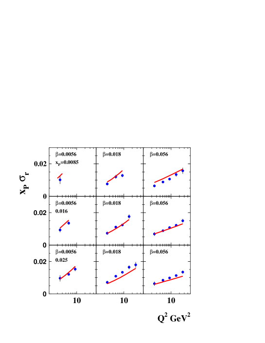
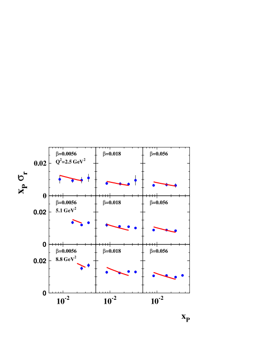
Fig. 6-a	Fig. 6-b

Figure 6: $\sigma^{\rm diff}\left(Y,Y_{0},Q^{2}\right)=x_{I\!\!P}\,\sigma_{r}$ versus $Q^{2}$ at fixed $\beta$ and $x_{I\!\!P}$ (Fig. 6-a) and versus $x_{I\!\!P}$ at fixed $\beta$ and $Q^{2}$ (Fig. 6-b). The data are taken from Ref.HERADATA . The red curves show the results of the fit with $m_{1}=Q_{s}\left(Y_{0},b\right)$. The fit in which $m_{1}$ was a fitted parameter turns out to be so close to this fit that cannot be clearly shown in the picture in spite of the fact that has higher value of $\chi^{2}/d.o.f.$.

We do not expect a good description of the data as we have mentioned. As was expected the values of parameter $\lambda_{1}$ turns out to be quite different from the leading order estimates in perturbative QCD, which illustrate the need for the next to leading order corrections. We notice that in the experimental kinematic region $\tau_{D}=r^{2}Q^{2}\left(Y-Y_{0},\boldsymbol{b}-\boldsymbol{b}^{\prime}\right)\,\leq\,1$. Therefore, the most data are in the region which is outside of the saturation domain. Hence, Eq. (37) and Eq. (101), which sums the emission of several gluons in perturbative QCD, has to be tried to describe the data. The success of the simple model for diffraction production: production of $q\bar{q}$ and $q\bar{q}G$ statesGBKW ; GOLEDD ; SATMOD0 ; KOML ; MUSCH ; MASC ; MAR ; KLMV , indicates, that taking into account the emission of several gluons, we will be able to describe the data. We are going to try in a separate further publications. On the other hand we see that the main contribution stems from the gluon emission. Indeed, in Fig. 7 we plot the two different terms of Eq. (66) writing it as $n^{D}=n^{D}_{1}+n^{D}_{2}$ where $n^{D}_{2}\propto N^{2}_{el}$. One can see that the emission of gluons (the term $n^{D}_{1}$) is certainly larger than the contribution of the diffractive production of quark-antiquark state (term $n^{D}_{2}$). We view this fact as an argument that we have to take into account a large number of emitted gluons.

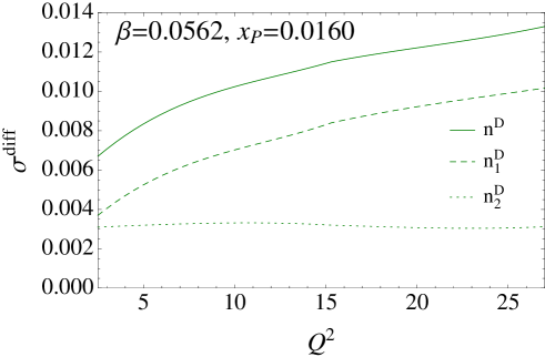
Figure 7: Contributions of two different sources of the diffractive production: the production of quark-antiquark state ($n^{D}_{2}$) and the multi-gluon production ($n^{D}_{1}$).

It should be mentioned that we have some hidden parameters which mostly specify the region of the applicability of the perturbative QCD estimates. For example, even in the case of deep inelastic processes, we can trust the wave function of perturbative QCD only, at rather large values of $Q^{2}\,\geq\,Q^{2}_{0}$ with $Q^{2}_{0}\approx 0.7GeV^{2}$ since for smaller $Q$ it will be affected by the non-perturbative contributions. As we have mentioned that we consider the matching point $z_{m}$ of Eq. (78) as a fitting parameter due to a large uncertainty in the calculation of $B$ given by Eq. (77). From the fit we specify them as $\beta\,\leq\,0.056$,$x_{I\!\!P}\,\leq 0.025$, $0.7\leq Q^{2}\leq 27\,GeV^{2}$. We found that the fit does not depend on the value of the matching point $z_{m}$. This confirms that the data are outside of the saturation region.

IV Conclusions

In the paper we discussed the evolution equations for the diffractive production in the framework of CGC/saturation approach that have been proposed in Ref.KOLE and found the analytical solutions in the several kinematic regions. The most impressive features of these solutions are that the diffractive production does not show the geometric scaling behaviour being a function of one variable. Even deep in the saturation regions for both diffractive and elastic amplitude the solution turns out to be the product of two functions: one has a geometric scaling behaviour depending on one variable $z$, and the second depends on $z_{0}$ showing the geometric scaling behaviour in the same way as elastic scattering amplitude at $Y-Y_{0}$.

Based on these solutions we suggest a impact parameter dependent saturation model which is suited for the describing the diffraction production both deep in the saturation region and in the vicinity of the saturation scale. Since we are dealing in the diffraction production with two saturation scales: $Q\left(Y,b\right)$ and $Q\left(Y-Y_{0},\boldsymbol{b}-\boldsymbol{b}^{\prime}\right)$, where $Y=\ln(1/(x_{I\!\!P}\beta)$ and $Y_{0}=\ln(1/\beta)$, the model includes more information from the theoretical part of the paper than it has been needed for the inclusive DIS. However, the main key assumptions of the model are the same as for inclusive DIS: the non-perturbative impact parameter behavior is absorbed into two saturation scales.

Using the model we tried to fit the combined data on diffraction production from H1 and ZEUS collaborationsHERADATA . We fond that we are able describe both $x_{I\!\!P}$ and $\beta$ dependence as well as $Q$ behavior of the measured cross sections. In spite of the sufficiently large $\chi^{2}/d.o.f.$ we believe that our description give the starting impetus to find a fit of the experimental data based on the solution of the CGC/saturation equation rather than on describing the diffraction system in smlistic way assuming that onle quark=antiquark pair and one extra gluons are produced.

Ae the result of the fit we found out that the experimental data are concentrated in the region outside the saturation domain for the produced diffractive system and we intend to try to sum the multi-gluon production in perturbative QCD approach using the formulae which we found in this paper. We are going to publish the result of this kind of approach elsewhere.

We believe that this paper will revive the interest to the process of the diffractive production which is a unique process which description needs the understanding both the multi-particle generation process and the elastic (diffractive) rescattering at high energy.

V Acknowledgements

We thank our colleagues at Tel Aviv university and UTFSM for encouraging discussions. Our special thanks go to Asher Gotsman, Alex Kovner and Misha Lublinsky for elucidating discussions on the subject of this paper.

This research was supported by the BSF grant 2012124, by Proyecto Basal FB 0821(Chile), Fondecyt (Chile) grants 1140842, 1170319 and 1180118 and by CONICYT grant PIA ACT1406.

Appendix A Solution for $\delta Y\ll 1$ but $\bar{\alpha}_{S}\xi\sim 1$.

In this appendix we obtain the cross section for the diffractive production in the kinematic region, where $r^{2}Q^{2}_{s}(Y_{0},b)\approx 1$ and $\delta Y\ll 1$, but do not use the assumption, that $\bar{\alpha}_{S}\xi\gg 1$ which we used in section IIC-3. As in this section we are dealing with the integral

$${\sum_{n=0}^{\infty}(\bar{\alpha}_{S}\delta Y)^{n}\int_{C_{3}}\frac{d\gamma}{2\pi i}\dfrac{1}{\gamma^{n}}\dfrac{e^{(\gamma-1)\xi}}{\gamma-\tilde{\gamma}}.}$$ (88)

We wish to calculate this integral using the special function in the most compact and economic way. First, we note that for $n=0$ we can take the integral closing the contour of the integration over the pole $\gamma=\tilde{\gamma}$. For each $n\geq 1$, we can write the contribution as the convolution integral

$${\int_{C_{3}}\frac{d\gamma}{2\pi i}\dfrac{1}{\gamma^{n}}\dfrac{e^{(\gamma-1)\xi}}{\gamma-\tilde{\gamma}}}\,\,=\,\,\displaystyle{e^{\tilde{\gamma}-1}\int_{x}^{1}\dfrac{1}{\Gamma(n)}(-\ln(t))^{n-1}t^{\tilde{\gamma}}\dfrac{dt}{t}},$$ (89)

with $x=e^{-\xi}$.

Plugging (89) into (88) we obtain the following expression

$$n^{D}(Y,Y_{0},\xi,b)\,=\,\,C\left(Y_{0},b\right)\,e^{(\tilde{\gamma}-1)\xi}\left(1+\displaystyle{\int_{x}^{1}\dfrac{\bar{\alpha}_{S}\delta Y}{\sqrt{\bar{\alpha}_{S}\delta Y\ln(1/t)}}I_{1}(2\sqrt{\bar{\alpha}_{S}\delta Y\ln(1/t)})t^{\tilde{\gamma}}\dfrac{dt}{t}}\right).$$ (90)

with

$$C\left(Y_{0},b\right)\,\,=\,\,2\bar{\alpha}_{S}\,\bar{\gamma}\,\kappa\,c^{2}\,\left(\frac{Q^{2}\left(Y_{0},b\right)}{Q^{2}_{s}\left(Y_{\rm in}\right)}\right)^{2\bar{\gamma}}$$ (91)

The next step is to express the integral on the r.h.s. in term of Lommel’s function. Using that

$$\dfrac{d}{dt}I_{0}(2\sqrt{\bar{\alpha}_{S}\delta Y\ln(1/t)})=-\dfrac{\bar{\alpha}_{S}\delta Y}{\sqrt{\bar{\alpha}_{S}\delta Y\ln(1/t)}}I_{1}(2\sqrt{\bar{\alpha}_{S}\delta Y\ln(1/t)})\dfrac{1}{t}.$$ (92)

the expression in (90) can be written as follows

$$n^{D}(Y,Y_{0},\xi,b)\,=\,C\left(Y_{0},b\right)\,e^{(\tilde{\gamma}-1)\xi}\left(1+\displaystyle{\int_{x}^{1}\dfrac{d}{dt}I_{0}(2\sqrt{\bar{\alpha}_{S}\delta Y\ln(1/t)})t^{\tilde{\gamma}}dt}\right).$$ (93)

Taking integration by parts into (93) we obtain

$$n^{D}(Y,Y_{0},\xi,b)\,=\,C\left(Y_{0},b\right)\,e^{-\xi}I_{0}(2\sqrt{\bar{\alpha}_{S}\delta Y\xi})+\tilde{\gamma}e^{(\tilde{\gamma}-1)\xi}\int_{x}^{1}I_{0}(2\sqrt{\bar{\alpha}_{S}\delta Y\ln(1/t)})t^{\tilde{\gamma}}\dfrac{dt}{t}.$$ (94)

Using $u=\sqrt{\ln(1/t)/\ln(1/x)}$, the integral in the above expression can be rewritten as

$$n^{D}(Y,Y_{0},\xi,b)=e^{-\xi}I_{0}(2\sqrt{\bar{\alpha}_{S}\delta Y\xi})+2\tilde{\gamma}\xi e^{-\xi}\int_{0}^{1}e^{\tilde{\gamma}\xi(1-u^{2})}I_{0}(2\sqrt{\bar{\alpha}_{S}\delta Y}u)udu.$$ (95)

Introducing $z=2i\sqrt{\bar{\alpha}_{S}\delta Y\xi}$, $w=-2i\tilde{\gamma}\xi$ into (95) yields the following representation

$$n^{D}(Y,Y_{0},\xi,b)=\,C\left(Y_{0},b\right)\,\Bigg{(}e^{-\xi}I_{0}(2\sqrt{\bar{\alpha}_{S}\delta Y\xi})+e^{-\xi}\dfrac{1}{i}\left(U_{1}(w,z)-iU_{2}(w,z)\right)\Bigg{)},$$ (96)

where $U_{\nu}(w,z)$ denotes the Lommel function of two variables. The series representation

$$\begin{array}[]{rcl}U_{1}(w,z)&=&i\displaystyle{\sum_{m=0}^{\infty}\left(-\dfrac{\tilde{\gamma}\xi}{\sqrt{\bar{\alpha}_{S}\delta Y\xi}}\right)^{2m+1}I_{2m+1}(2\sqrt{\bar{\alpha}_{S}\delta Y\xi})}\\ U_{2}(w,z)&=&-\displaystyle{\sum_{m=0}^{\infty}\left(-\dfrac{\tilde{\gamma}\xi}{\sqrt{\bar{\alpha}_{S}\delta Y\xi}}\right)^{2m+2}I_{2m+2}(2\sqrt{\bar{\alpha}_{S}\delta Y\xi})}\end{array}$$ (97)

becomes

$$n^{D}(Y,Y_{0},\xi,b)=\,C\left(Y_{0},b\right)\,\left(e^{-\xi}I_{0}(2\sqrt{\bar{\alpha}_{S}\delta Y\xi})+e^{-\xi}\displaystyle{\sum_{m=1}^{\infty}(-1)^{m}\left(-\dfrac{\tilde{\gamma}\xi}{\sqrt{\bar{\alpha}_{S}\delta Y\xi}}\right)^{m}I_{m}(2\sqrt{\bar{\alpha}_{S}\delta Y\xi})}\right).$$ (98)

As $\xi\gg 1$, the expression (98) it is not a suitable representation for the asymptotic analysis. This problem is resolved considering the generating function of the Bessel functions that can be written as follows

$$e^{(z/2)\left(t+t^{-1}\right)}=\displaystyle{\sum_{m=-\infty}^{\infty}t^{m}I_{m}(z)}$$ (99)

Introducing Eq. (99) into Eq. (98), and using that $I_{m}(z)=I_{-m}(z)$, we obtain

$$n^{D}(Y,Y_{0},\xi,b)=\,C\left(Y_{0},b\right)\,\left(e^{(\tilde{\gamma}-1)\xi+\dfrac{\bar{\alpha}_{S}\delta Y}{\tilde{\gamma}}}-\displaystyle{e^{-\xi}\sum_{m=1}^{\infty}\left(\dfrac{1}{\tilde{\gamma}}\sqrt{\dfrac{\bar{\alpha}_{S}\delta Y}{\xi}}\right)^{m}I_{m}(2\sqrt{\bar{\alpha}_{S}\delta Y\xi}).}\right)$$ (100)

At large $\bar{\alpha}_{S}\delta Y\xi$, Eq. (100) takes the form

$$n^{D}(Y,Y_{0},\xi,b)=\,C\left(Y_{0},b\right)\,\left(e^{(\tilde{\gamma}-1)\xi+\dfrac{\bar{\alpha}_{S}\delta Y}{\tilde{\gamma}}}-2\sqrt{\pi}\displaystyle{\left(\dfrac{(\bar{\alpha}_{S}\delta Y)^{3}}{\xi}\right)^{1/4}\dfrac{e^{-\xi+2\sqrt{\bar{\alpha}_{S}\delta Y\xi}}}{\tilde{\gamma}-\sqrt{\bar{\alpha}_{S}\delta Y/\xi}}.}\right)$$ (101)

One can see that this equation coincides with Eq. (37) if we replace $\chi\left(\gamma\right)$ by $1/\gamma$ and consider $\sqrt{\bar{\alpha}_{S}\delta Y/\xi}$ being much larger than $\tilde{\gamma}$.

References

- (1) Yuri V Kovchegov and Eugene Levin, “ Quantum Choromodynamics at High Energies", Cambridge Monographs on Particle Physics, Nuclear Physics and Cosmology, Cambridge University Press, 2012 .
- (2) Y. V. Kovchegov and E. Levin, Nucl. Phys. B 577 (2000) 221, [hep-ph/9911523].
- (3) M. Hentschinski, H. Weigert and A. Schafer, Phys. Rev. D 73 (2006) 051501, [hep-ph/0509272].
- (4) Y. Hatta, E. Iancu, C. Marquet, G. Soyez and D. N. Triantafyllopoulos, Nucl. Phys. A 773 (2006) 95, [hep-ph/0601150].
- (5) A. Kovner, M. Lublinsky and H. Weigert, Phys. Rev. D 74 (2006) 114023, [hep-ph/0608258].
- (6) K. J. Golec-Biernat and J. Kwiecinski, Phys. Lett. B 353 (1995) 329, [hep-ph/9504230].
- (7) E. Gotsman, E. Levin and U. Maor, Nucl. Phys. B 493 (1997) 354, [hep-ph/9606280].
- (8) K. J. Golec-Biernat and M. Wusthoff, Phys. Rev. D 60 (1999) 114023 [hep-ph/9903358]; Phys. Rev. D 59 (1998) 014017; [hep-ph/9807513].
- (9) Y. V. Kovchegov and L. D. McLerran, Phys. Rev. D 60 (1999) 054025 Erratum: [Phys. Rev. D 62 (2000) 019901], [hep-ph/9903246].
- (10) S. Munier and A. Shoshi, Phys. Rev. D 69 (2004) 074022, [hep-ph/0312022].
- (11) C. Marquet and L. Schoeffel, Phys. Lett. B 639 (2006) 471, [hep-ph/0606079].
- (12) C. Marquet, Phys. Rev. D 76 (2007) 094017, [arXiv:0706.2682 [hep-ph]].
- (13) H. Kowalski, T. Lappi, C. Marquet and R. Venugopalan, Phys. Rev. C 78 (2008) 045201, [arXiv:0805.4071 [hep-ph]].
- (14) E. Levin and M. Lublinsky, Nucl. Phys. A 712 (2002) 95, [hep-ph/0207374].
- (15) E. Levin and M. Lublinsky, Eur. Phys. J. C 22 (2002) 64, [hep-ph/0108239].
- (16) C. Contreras, E. Levin, R. Meneses and I. Potashnikova, Phys. Rev. D 94 (2016) no.11, 114028; [arXiv:1607.00832 [hep-ph]].
- (17) C. Contreras, E. Levin and I. Potashnikova, Nucl. Phys. A 948 (2016) 1, [arXiv:1508.02544 [hep-ph]].
- (18) E. Levin and K. Tuchin, Nucl. Phys. B 573, 833 (2000) [hep-ph/9908317]; Nucl. Phys. A 691, 779 (2001) [hep-ph/0012167]; 693, 787 (2001) [hep-ph/0101275].
- (19) E. Iancu, K. Itakura and S. Munier, Phys. Lett. B 590 (2004) 199 [hep-ph/0310338].
- (20) C. Contreras, E. Levin and R. Meneses, JHEP 1410 (2014) 138 [arXiv:1406.1212 [hep-ph]].
- (21) A. Kovner and U. A. Wiedemann, Phys. Rev. D 66, 051502 (2002) [hep-ph/0112140]; Phys. Rev. D 66, 034031 (2002) [hep-ph/0204277]; Phys. Lett. B 551, 311 (2003) [hep-ph/0207335].
- (22) J. Bartels, K. J. Golec-Biernat and H. Kowalski, Phys. Rev. D 66 (2002) 014001 [hep-ph/0203258].
- (23) S. Bondarenko, M. Kozlov and E. Levin, Nucl. Phys. A 727 (2003) 139 [hep-ph/0305150].
- (24) H. Kowalski and D. Teaney, Phys. Rev. D 68 (2003) 114005 [hep-ph/0304189].
- (25) H. Kowalski, L. Motyka and G. Watt, Phys. Rev. D 74 (2006) 074016 [hep-ph/0606272].
- (26) H. Kowalski, T. Lappi and R. Venugopalan, Phys. Rev. Lett. 100 (2008) 022303 [arXiv:0705.3047 [hep-ph]].
- (27) H. Kowalski, T. Lappi, C. Marquet and R. Venugopalan, Phys. Rev. C 78 (2008) 045201 [arXiv:0805.4071 [hep-ph]].
- (28) G. Watt and H. Kowalski, Phys. Rev. D 78 (2008) 014016 [arXiv:0712.2670 [hep-ph]].
- (29) E. Levin and A. H. Rezaeian, Phys. Rev. D 82 (2010) 014022 [arXiv:1005.0631 [hep-ph]].
- (30) A. H. Rezaeian, Phys. Lett. B 718 (2013) 1058 [arXiv:1210.2385 [hep-ph]].
- (31) E. Levin and A. H. Rezaeian, Phys. Rev. D 83 (2011) 114001 [arXiv:1102.2385 [hep-ph]].
- (32) E. Levin and A. H. Rezaeian, Phys. Rev. D 82 (2010) 054003 [arXiv:1007.2430 [hep-ph]].
- (33) D. Boer, M. Diehl, R. Milner, R. Venugopalan, W. Vogelsang, D. Kaplan, H. Montgomery and S. Vigdor et al., arXiv:1108.1713 [nucl-th].
- (34) T. Lappi and H. Mantysaari, Phys. Rev. C 83 (2011) 065202 [arXiv:1011.1988 [hep-ph]].
- (35) T. Toll and T. Ullrich, Phys. Rev. C 87 (2013) 2, 024913 [arXiv:1211.3048 [hep-ph]].
- (36) P. Tribedy and R. Venugopalan, Nucl. Phys. A 850 (2011) 136 [Nucl. Phys. A 859 (2011) 185] [arXiv:1011.1895 [hep-ph]].
- (37) P. Tribedy and R. Venugopalan, Phys. Lett. B 710 (2012) 125 [Phys. Lett. B 718 (2013) 1154] [arXiv:1112.2445 [hep-ph]].
- (38) A. H. Rezaeian, M. Siddikov, M. Van de Klundert and R. Venugopalan, PoS DIS 2013 (2013) 060 [arXiv:1307.0165 [hep-ph]]; Phys. Rev. D 87 (2013) 3, 034002 [arXiv:1212.2974].
- (39) A. H. Rezaeian and I. Schmidt, Phys. Rev. D 88 (2013) 074016 [arXiv:1307.0825 [hep-ph]].
- (40) F. D. Aaron et al. [H1 and ZEUS Collaborations], Eur. Phys. J. C 72 (2012) 2175, [arXiv:1207.4864 [hep-ex]].
- (41) E. Ferreiro, E. Iancu, K. Itakura and L. McLerran, Nucl. Phys. A 710, 373 (2002) [hep-ph/0206241].
-
(42)
M. Froissart,
Phys. Rev. 123 (1961) 1053;
A. Martin, “Scattering Theory: Unitarity, Analitysity and Crossing." Lecture Notes in Physics, Springer-Verlag, Berlin-Heidelberg-New-York, 1969. - (43) G. P. Lepage and S. J. Brodsky, Phys. Rev. Lett. 43 (1979) 545; Phys. Rev. Lett. 43 (1979) 1625.
- (44) I. Balitsky, [arXiv:hep-ph/9509348]; Phys. Rev. D60, 014020 (1999) [arXiv:hep-ph/9812311]; Y. V. Kovchegov, Phys. Rev. D60, 034008 (1999), [arXiv:hep-ph/9901281].
- (45) J. Bartels, E. Levin, Nucl. Phys. B387 (1992) 617-637; A. M. Stasto, K. J. Golec-Biernat, J. Kwiecinski, Phys. Rev. Lett. 86 (2001) 596-599, [hep-ph/0007192]; L. McLerran, M. Praszalowicz, Acta Phys. Polon. B42 (2011) 99, [arXiv:1011.3403 [hep-ph]] B41 (2010) 1917-1926, [arXiv:1006.4293 [hep-ph]]; M. Praszalowicz, Acta Phys. Polon. B 42 (2011) 1557 [arXiv:1104.1777 [hep-ph]]; M. Praszalowicz and T. Stebel, JHEP 1303 (2013) 090 [arXiv:1211.5305 [hep-ph]]; L. McLerran, M. Praszalowicz and B. Schenke, Nucl. Phys. A 916 (2013) 210 [arXiv:1306.2350 [hep-ph]]; M. Praszalowicz, Phys. Lett. B 727 (2013) 461 [arXiv:1308.5911 [hep-ph]]; L. McLerran and M. Praszalowicz, Phys. Lett. B 741 (2015) 246 [arXiv:1407.6687 [hep-ph]].
- (46) E. Iancu, K. Itakura and L. McLerran, Nucl. Phys. A 708 (2002) 327 [hep-ph/0203137].
- (47) A. H. Mueller and D. N. Triantafyllopoulos, Nucl. Phys. B 640 (2002) 331 [hep-ph/0205167];
- (48) I. Gradstein and I. Ryzhik, Table of Integrals, Series, and Products, Fifth Edition, Academic Press, London, 1994.
- (49) A. Polyanin, A. Manzhinov, Handbook of integral equations Second edition, Chapman Hall/CRC Taylor Francis Group
- (50) G. N. Watson, A tratise on the theory of Bessel function, Cambridge University Press