Efficiency and power of minimally nonlinear irreversible heat engines with broken time-reversal symmetry

Abstract

We study the minimally nonlinear irreversible heat engines in which the time-reversal symmetry for the systems may be broken. The expressions for the power and the efficiency are derived, in which the effects of the nonlinear terms due to dissipations are included. We show that, as within the linear responses, the minimally nonlinear irreversible heat engines enable attainment of Carnot efficiency at positive power. We also find that the Curzon-Ahlborn limit imposed on the efficiency at maximum power can be overcomed if the time-reversal symmetry is broken.

PACS number(s): 05.70.Ln

I Introduction

Heat engines as energy converters provide a good platform for studying the nature of thermodynamics, in addition to its relation with utilization of energy resources. Exploring the efficient heat engines at large power is therefore an issue of significance in thermodynamics. The second law of thermodynamics tells us that the efficiency of a heat engine working between two heat reservoirs of constant temperatures $T_{h}$ and $T_{c}(<T_{h})$ is bounded by the Carnot efficiency $\eta_{C}=1-T_{c}/T_{h}$. As the Carnot engine needs infinite time for completing a cycle and produces null power, practically a heat engine needs to be speeded up. Starting with Curzon and Ahlborn model Cur75 , the issue of the efficiency at maximum power and its possible universal bounds was intensively studied in the literature Wu04 ; Tu14 ; Liu15 ; Hol16 ; Sei17 ; Bro05 ; Bra15 ; Esp09 ; Esp10 ; Wang15 ; Wang14 ; Rez06 ; Ape12 ; Gon17 ; Fel03 ; Chen13 ; Bai18 ; Abah12 . Another increasing interesting topic is the attainable maximum efficiency at nonvanishing power for the heat engines and it has attracted much attention recently Ben11 ; All13 ; Whit14 ; Pol15 ; Pro15 ; Joh17 ; Lee17 ; Cam16 .

In the seminal paper Ben11 the bounds on efficiency for a specific model of steady state heat engine with broken time-reversal symmetry caused, for example, by an external magnetic field were investigated. It was shown that, within the linear response regime, this time-reversal antisymmetry can significantly boost the performance and enable attainment of Carnot limit at nonzero power. The performance of the steady state heat engine working in the linear response regime, with broken time-reversal symmetry, raised issues that deserve to be addressed. For instance, is there the improvement of performance in cyclic heat engines induced by broken time-reversal symmetry? Can heat engines beyond the linear response regime allow the Carnot limit at positive power, with or without broken time-reversal symmetry? How to identify the relations between the power, efficiency, and unavoidable dissipations? The time-reversal symmetry was found to boost the performance of cyclic heat engines in the linear responses Pro15 ; Bra15 . The general relations between the efficiency, power and dissipations were analyzed in the regimes of linear Jiang14 ; Bau16 ; Pro16 and nonlinear Iyy18 responses. In another recent paper Cam16 , the attainable maximum efficiency of heat engines is studied that does not require broken time-reversal symmetry. It was found that enhancement of specific heat via phase transition can significantly boost the performance of a heat engine and enable the realization of Carnot limit at nonzero power, even beyond linear response regime.

In the present paper, we investigate the questions of whether the maximum efficiency can approach the Carnot limit at positive power and whether the Curzon-Ahlborn limit for the efficiency at maximum power can be exceeded in the nonlinear response regime. We propose a minimally nonlinear irreversible heat engine Izu12 , in which the local dissipations are included Izu12 ; Izu13 , and study its efficiency and power for the case of broken time-reversal symmetry. We show that the maximum efficiency can reach the Carnot value at nonzero power and the Curzon-Ahlborn limit on the efficiency at maximum power is overcomed in the time-reversal antisymmetry.

II minimally nonlinear irreversible heat engine with Broken Time-Reversal Symmetry

The heat engine model under consideration, which may be cyclic or steady state and where broken time-reversal symmetry may be induced, for instance, by interaction with an external magnetic field B. The working substance is in contact with a hot reservoir and a cold one of temperatures $T_{h}$ and $T_{c}(<T_{h})$. In order to describe the minimally nonlinear irreversible heat engines in which only a second-order nonlinear term is added in the linear Onsager relations to describe the inevitable dissipations, we adopt the extended Onsager relations Izu12 ; Izu13 with inclusion of external field B,

$$J_{1}(\textbf{B})=L_{11}(\textbf{B})X_{1}+L_{12}(\textbf{B})X_{2},,$$ (1)

$$J_{2}(\textbf{B})=L_{21}(\textbf{B})X_{1}+L_{22}(\textbf{B})X_{2}-\gamma_{h}J_{1}^{2}(\textbf{B}),$$ (2)

where the nonlinear term $\gamma_{h}J_{1}^{2}$ denotes heat dissipation into the hot reservoir and ${\gamma_{h}(\geq 0)}$ indicates the dissipation strength. Noteworthy, the time-reversal symmetry will be broken due to the external field B, thereby leading to the Onsager coefficients $L_{12}(\textbf{B})\neq L_{21}(\textbf{B})$ for the heat engines under consideration, though the Onsager-Casimir relation $L_{12}(\textbf{B})=L_{21}(-\textbf{B})$ is satisfied. For sake of convenience, the following formula will include the external field but without explicitly writing B.

In the heat engine the heat flux $\dot{Q}_{h}$ is extracted from the hot heat reservoir at the temperature $T_{h}$, and there must be a certain heat current $\dot{Q}_{c}$ injected to the cold heat reservoir of temperature $T_{c}$, with corresponding production of power output $P=\dot{Q}_{h}+\dot{Q}_{c}$. Throughout the paper the dot means the quantity per unit time for steady-state heat engines or the quantity divided by the cycle time duration for cyclic machines. Since the entropy production of a steady-state or a cyclic heat engine merely contributed from the two heat reservoirs, and its rate thus reads

$$\dot{\sigma}=-\left(\frac{\dot{Q_{h}}}{T_{h}}+\frac{\dot{Q_{c}}}{T_{c}}\right)=-\frac{P}{T_{c}}+\dot{Q_{h}}\left(\frac{1}{T_{c}}-\frac{1}{T_{h}}\right).$$ (3)

Without loss of generality, the power output $P$ can be expressed as $P=F\dot{x}$, where $F$ is an external force and $x$ is its corresponding thermodynamically conjugate variable. As the entropy production rate can be expressed in terms of the thermodynamic fluxes J and forces X: $\dot{\sigma}=\textbf{J}\textbf{X}$, from Eq. (3) we have

$$\dot{\sigma}=J_{1}X_{1}+J_{2}X_{2}$$ (4)

through defining the thermodynamic fluxes $J_{1}\equiv\dot{x}$ and $J_{2}\equiv\dot{Q_{h}}$, with conjugate affinities $X_{1}=F/T_{c}$ and $X_{2}=1/T_{c}-1/T_{h}$. The power output can thus be expressed as

$$P=-J_{1}X_{1}T_{c}.$$ (5)

Based on Eqs. (1) and (2), we can rewrite $J_{2}$ as

$$J_{2}=\frac{L_{21}}{L_{11}}J_{1}+L_{22}\left(1-\frac{L_{12}L_{21}}{L_{11}L_{22}}\right)X_{2}-\gamma_{h}J_{1}^{2}.$$ (6)

Let $J_{3}\equiv\dot{Q}_{c}$, we have $J_{3}=\dot{Q_{h}}-P=J_{1}X_{1}T_{c}+J_{2},$ which takes the form of

$$J_{3}=\frac{L_{21}-L_{12}X_{2}T_{c}}{L_{11}}J_{1}+L_{22}\left(1-\frac{L_{12}L_{21}}{L_{11}L_{22}}\right)X_{2}-\gamma_{c}J_{1}^{2},$$ (7)

where $\gamma_{c}=T_{h}/L_{11}-\gamma_{h}$ has been used and it represents the strength of the power dissipation into the cold reservoir. With consideration of Eqs. (1), (4) and (6), we find that the Onsager coefficients must be constrained by

$$L_{11}\geq 0,~{}L_{22}\geq 0,~{}L_{11}L_{22}-{L_{11}L_{22}\alpha\eta_{C}}-{(L_{12}+L_{21})^{2}}/{4}+{L_{12}L_{21}\alpha\eta_{C}}\geq 0,$$ (8)

due to the nonnegativity of the entropy production rate ($\dot{\sigma}\geq 0)$. Here and hereafter we define $\alpha\equiv 1/(1+\gamma_{c}/\gamma_{h})$ and take $\alpha$ rather than $\gamma_{c}/\gamma_{h}$ as the dissipation ratio for simplicity. The asymmetric dissipation limits $\gamma_{c}/\gamma_{h}\rightarrow\infty$ and $\gamma_{c}/\gamma_{h}\rightarrow 0$ correspond to $\alpha=0$ and $\alpha=1$, respectively. The symmetrical dissipation case when $\gamma_{h}=\gamma_{c}$ leads to $\alpha=1/2$. When the entropy production rate tends to be zero ($\dot{\sigma}=0$), we have $L_{11}L_{22}-{L_{11}L_{22}\alpha\eta_{C}}-{(L_{12}+L_{21})^{2}}/{4}+{L_{12}L_{21}\alpha\eta_{C}}=0.$

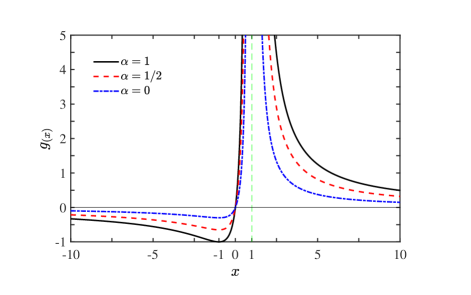
Figure 1: The function $g(x)$ as a function of the asymmetry parameter $x$, with dissipation parameter $\alpha=1$ (black solid line), $\alpha=1/2$ (red dashed line), and $\alpha=0$ (blue dot-dashed line). The vertical asymptote of $g(x)$ at $x=1$ is indicated by green dotted line (When $\alpha\neq 0$, $\eta_{C}=0.7$ is adopted).

III maximum efficiency

As the efficiency $\eta$ takes the form of

$$\eta=\frac{P}{J_{2}}=\frac{-J_{1}X_{1}T_{c}}{L_{21}X_{1}+L_{22}X_{2}-\gamma_{h}(L_{11}X_{1}+L_{12}X_{2})^{2}}.$$ (9)

the derivation of $\eta$ with respect to $X_{1}$ gives rise to the expression of the maximum efficiency,

$$\eta_{\mathrm{max}}=\eta_{C}\frac{y+2-2\sqrt{y+1-\alpha\eta_{C}yx}}{4\alpha\eta_{C}+{y}/{x}},$$ (10)

at the thermodynamic force

$$X_{1}=\frac{L_{11}X_{2}(L_{22}-L_{12}^{2}X_{2}\gamma_{h})-\sqrt{L_{11}(L_{11}L_{22}-L_{12}L_{21})X_{2}^{2}(L_{22}-L_{12}^{2}X_{2}\gamma_{h})}}{L_{11}(-L_{21}+L_{11}L_{12}X_{2}\gamma_{h})},$$ (11)

where we have introduced two parameters $x={L_{12}}/{L_{21}},$ and $y={L_{12}L_{21}}/{(L_{11}L_{22}-L_{12}L_{21})}.$

Since no restriction is imposed on the attainable values of the asymmetry parameter $x$, the relation (8) yields

$$g(x)\leq y\leq 0~{}~{}~{}~{}~{}(x\leq 0),$$ (12a)

$$0\leq y\leq g(x)~{}~{}~{}~{}~{}(x>0),$$ (12b)

where we have defined

$$g(x)\equiv\frac{4(1-\alpha\eta_{C})x}{(x-1)^{2}}.$$ (13)

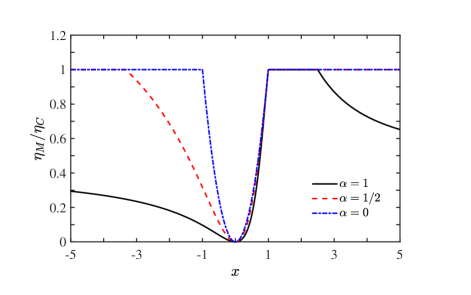
Figure 2: (Color online) Ratio $\eta_{M}/\eta_{C}$ as a function of the asymmetry parameter $x$. The dissipation ratios are $\alpha=1$ (black solid line), $\alpha=1/2$ (red dashed line), and $\alpha=0$ (blue dot-dahsed line) (when $\alpha\neq 0$, $\eta_{C}=0.7$ is adopted).

It reduces to $g(x)=4x/(x-1)^{2}$ obtained in the linear response regime Ben11 , if the dissipation vanishes $\gamma_{h}\rightarrow 0$ as well as $\alpha\rightarrow 0$. We stress that direct use of $g(x)=4x/(x-1)^{2}$ as done in Ref. Bai18 would yield nonphysical, negative entropy production rate for the nonlinear case with $\alpha\neq 0$. The effects of nonvanishing dissipation ($\alpha\neq 0)$ on the bound function $g(x)$ are of significance for any $x$, as shown in Fig. 1. For a given asymmetry parameter $x$, the maximum value $\eta_{\mathrm{M}}$ of Eq. (10) is achieved if $y=h(x)$. Considering Eqs. (12) and (13), we can obtain the maximum efficiency $\eta_{\mathrm{M}}$ via simple algebra as follows: (1) when $\alpha\eta_{C}\leq 1/2$,

$$\eta_{\mathrm{M}}= \eta_{C}\frac{x^{2}(1-\alpha\eta_{C})}{(x-2)x\alpha\eta_{C}+1} (\frac{1}{2\alpha\eta_{C}-1}\leq x\leq 1)$$ , (14a)

$$\eta_{\mathrm{M}}= \eta_{C} (x\leq\frac{1}{2\alpha\eta_{C}-1}~{}\mathrm{and}~{}x\geq 1)$$ , (14b)

and when $1/2<\alpha\eta_{C}\leq 1$,

$$\eta_{\mathrm{M}}= \eta_{C}\frac{x^{2}(1-\alpha\eta_{C})}{(x-2)x\alpha\eta_{C}+1} (x\geq\frac{1}{2\alpha\eta_{C}-1}~{}\mathrm{and}~{}x\leq 1)$$ , (15a)

$$\eta_{\mathrm{M}}= \eta_{C} (1\leq x\leq\frac{1}{2\alpha\eta_{C}-1})$$ . (15b)

If, in particular, $\alpha\rightarrow 0$ as the dissipation vanishes $\gamma_{h}\rightarrow 0$, Eqs. (14b) and (14a) simplify to

$$\eta_{\mathrm{M}}= \eta_{C}x^{2} (\big{|}x\big{|}\leq 1)$$ , (16a)

$$\eta_{\mathrm{M}}= \eta_{C} (\big{|}x\big{|}\geq 1)$$ , (16b)

which were obtained within the framework of linear irreversible thermodynamics Ben11 ; Bra15 . Besides $\eta_{C}$, the function depends on $\eta_{\mathrm{M}}$ both $x$ and $\alpha$ if the dissipation exists with $\alpha\neq 0$. For $\alpha\leq(2\eta_{C})^{-1}$, the Carnot efficiency can be approached when $x\geq 1$ and when $x\leq({2\alpha\eta_{C}-1})^{-1}$; whereas for $(2\eta_{C})^{-1}<\alpha\leq\eta_{C}^{-1}$, the range in which the Carnot limit is reached becomes $1\leq x\leq({2\alpha\eta_{C}-1})^{-1}$. The ratio $\eta_{\mathrm{M}}/\eta_{C}$ for different values of $\alpha$ is drawn in Fig. 2, where $\eta_{C}=0.7$ for $\alpha\neq 0$ is adopted. Let us consider two special cases: (1) when $\alpha=1$ and thus $\alpha\eta_{C}=0.7$, the Carnot limit is reached during the range of $1\leq x\leq 2.5$, and $\eta_{\mathrm{M}}=\eta_{C}\{3x^{2}/[1+0.7(x-2)x]\}$ when $x\geq 2.5$ or $x\leq 1$; (2) when $\alpha=1/2$ and $\alpha\eta_{C}=0.35$, the Carnot limit is obtained in the region of $x\leq-3.33$ and $x\geq 1$. The former and latter cases are indicted by the black solid line and the red dashed one, respectively, in Fig. 2 where the linear irreversible case ($\alpha=0$) is represented by the blue dot-dashed line. Since the Carnot efficiency is obtained under the condition $y=g(x)$, we find that $\mathrm{det}(\mathbf{L})=(L_{12}-L_{21})^{2}/[4(1-\alpha\eta_{C})]$, and the entropy production rate $\dot{\sigma}=0$. The Carnot limit and $L_{12}\neq L_{21}$ yields $\mathrm{det}(\mathbf{L})>0$, showing that the Carnot efficiency could be realized only in the non-tight coupling case.

We find from Eqs. (5) and (11) that the power at maximum efficiency reads

$$P_{m\eta}=\eta_{C}X_{2}L_{21}^{2}\frac{\big{|}\left(x-1\right)\left[\left(1-2\alpha\eta_{C}\right)x+1\right]\big{|}\left(\big{|}x-1\big{|}-\big{|}\left(1-2\alpha\eta_{C}\right)x+1\big{|}\right)^{2}}{16L_{11}\left(1-\alpha\eta_{C}\right)^{2}\left(1-\alpha\eta_{C}x\right)^{2}},$$ (17)

which is always positive and simplifies for $0\leq\alpha\eta_{C}\leq 1/2$ and $1/2<\alpha\eta_{C}\leq 1$ to

$$P_{m\eta}= \eta_{C}x^{2}X_{2}L_{21}^{2}\frac{(1-x)[(1-2\alpha\eta_{C})x+1]}{4L_{11}(1-\alpha\eta_{C}x)^{2}} (\frac{1}{2\alpha\eta_{C}-1}\leq x\leq 1)$$ , (18a)

$$P_{m\eta}= \eta_{C}X_{2}L_{21}^{2}\frac{(x-1)[(1-2\alpha\eta_{C})x+1]}{4L_{11}(1-\alpha\eta_{C})^{2}} (x\leq\frac{1}{2\alpha\eta_{C}-1}~{}\mathrm{and}~{}x\geq 1)$$ , (18b)

and

$$P_{m\eta}= \eta_{C}x^{2}X_{2}L_{21}^{2}\frac{(1-x)[(1-2\alpha\eta_{C})x+1]}{4L_{11}(1-\alpha\eta_{C}x)^{2}} (x\geq\frac{1}{2\alpha\eta_{C}-1}~{}\mathrm{and}~{}x\leq 1)$$ , (19a)

$$P_{m\eta}= \eta_{C}X_{2}L_{21}^{2}\frac{(x-1)[(1-2\alpha\eta_{C})x+1]}{4L_{11}(1-\alpha\eta_{C})^{2}} (1\leq x\leq\frac{1}{2\alpha\eta_{C}-1})$$ , (19b)

respectively. From Eqs. (14b), (15b), (18b), and (19b), we see that for $0\leq\alpha\eta_{C}\leq 1/2$ the Carnot efficiency is attained at positive power in the range of $x\geq 1$ and $x\leq(1-2\alpha\eta_{C})^{-1}$, and that for $1/2\leq\alpha\eta_{C}\leq 1$ the Carnot limit can also be reached with nonzero power if $1\leq x\leq{(2\alpha\eta_{C}-1)}^{-1}$. The special case of the linear response regime when $\alpha=0$ results into the fact that the Carnot efficiency is achieved only when $\big{|}x\big{|}\geq 1$, as expected. We emphasize here that the nonzero power at the Carnot efficiency is found by using $y=g(x)$, which implies vanishing entropy production rate ($\dot{\sigma}=0$).

IV efficiency at maximum power

We now turn to the maximum power output $P_{\mathrm{max}}$ and its corresponding efficiency $\eta_{mp}$. It follows, using Eq. (5) and setting $\partial P/\partial{X_{1}}=0$, that the power output achieves its maximum value,

$$P_{\mathrm{max}}=\frac{\eta_{C}L_{12}^{2}}{4L_{11}}X_{2},$$ (20)

at

$$X_{1}=-\frac{L_{12}}{2L_{11}}{X_{2}}.$$ (21)

Substituting Eq. (21) into Eq. (9), we find that the efficiency at maximum power is

$$\eta_{mp}=\frac{\eta_{C}}{2}\frac{2xy}{4+y(2-x\alpha\eta_{C})},$$ (22)

whose maximum value $\eta_{mp}^{*}$ is obtained when and only when $y=g(x)$. By substitution of Eq. (12) into Eq. (22) we then arrive at

$$\eta_{mp}^{*}=\eta_{C}\frac{1-\alpha\eta_{C}}{{(\alpha\eta_{C}-{x^{-1}})^{2}}-\alpha\eta_{C}+1}.$$ (23)

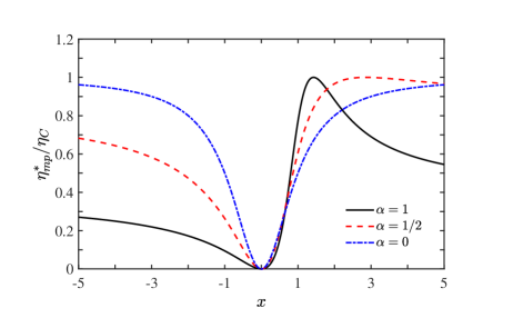
Figure 3: (Color online) Ratio $\eta_{mp}^{*}/\eta_{C}$ as a function of the asymmetry parameter $x$, with dissipation ratios $\alpha=1$ (black solid line), $\alpha=1/2$ (red dashed line) and $\alpha=0$ (blue dot-dashed line) (when $\alpha\neq 0$, $\eta_{C}=0.7$ is adopted).

We note that, for $x=1/(\alpha\eta_{C})$ or $\big{|}x\big{|}\rightarrow\infty$, $\eta_{mp}^{*}=\eta_{C}$, so the Carnot efficiency $\eta_{C}$ and the maximum power $P_{max}$ can be attained simultaneously. It is therefore indicated that the limit imposed on the efficiency at maximum power for systems with time-reversal symmetry is overcomed in the systems without this symmetry. If nonlinear term vanishes ($\gamma_{h}\rightarrow 0$ and $\alpha\rightarrow 0$), the efficiency at maximum power $\eta_{mp}^{*}=\eta_{C}x^{2}/(1+x^{2})$ in the linear situation is recovered and $\eta_{mp}^{*}\rightarrow\eta_{C}$ as $\big{|}x\big{|}\rightarrow\infty$. Figure 3 shows that the efficiency at maximum power $\eta_{mp}^{*}$ (for given $\alpha$) expressed by Eq. (23). Insight can be gained into the condition of attainment of the Carnot efficiency by seeing first from Fig. 3 that for $\alpha=1$ and $\eta_{C}=0.7$ efficiency at maximum power $\eta_{mp}^{*}=\eta_{C}$ can be achieved at the point $x=1/0.7\simeq 1.428$ (or $\big{|}x|\rightarrow\infty$ which is not shown in the figure). Second, from Fig. 1, we note that for $x<0$ the efficiency $\eta^{*}_{mp}$ increase more slowly to approach the Carnot limit in the minimally nonlinear response regime than in the linear response case.

We also emphasize that, for the time-reversal symmetry ($x=1$), the efficiency at maximum power (23) becomes

$$\eta^{*}_{mp}=\frac{\eta_{C}}{2-\alpha\eta_{C}},$$ (24)

which is situated between $\eta_{C}/2\leq\eta_{mp}^{*}\leq\eta_{C}/(2-\eta_{C})$ as $0\leq\alpha\leq 1$. The upper bounds and lower bounds were obtained earlier in the low-dissipation Carnot heat engines Esp10 and the minimally nonlinear irreversible heat engines Izu12 satisfying the tight-coupling condition at the asymmetrical dissipation limits. In the dissipation symmetric limit $\alpha=1/2$, we find that the maximum efficiency at maximum power is $\eta_{mp}^{*}=\eta_{C}/(2-\eta_{C}/2)$, and its expansion in terms of $\eta_{C}$ up to third order is $\eta_{mp}^{*}=\eta_{C}/2+\eta_{C}^{2}/8+3\eta_{C}^{3}/32+\mathcal{O}(\eta_{C}^{4})$, which agrees well with the expansion of the famous Curzon-Ahlborn efficiency, $\eta_{CA}=1-\sqrt{T_{c}/T_{h}}=\eta_{C}/2+\eta_{C}^{2}/8+\eta_{C}^{3}/16+\mathcal{O}(\eta_{C}^{4})$, indicating that they have the same universality of $\eta_{C}/2+\eta_{C}^{2}/8$.

V conclusions

For systems with broken time-reversal symmetry, we have investigated the performance of minimally nonlinear irreversible heat engines (based on these systems). For these nonlinear irreversible heat engines, the maximum efficiency can tend to be Carnot limit at nonzero power and efficiency at maximum power can go beyond the Curzon-Ahlborn limit when the asymmetric parameter $x$ satisfies a certain condition. Our results hold for both cyclic heat engines and steady state ones. Our analytical results provides a theoretical framework for understanding of minimally nonlinear heat engines, but should also be helpful for studying the heat devices in which higher nonlinear terms due to dissipations are involved.

Acknowledgements We acknowledge the financial support from NSFC(Grant Nos. 11505091, 11265010, and 11365015), the Major Program of Jiangxi Provincial NSF (Grant No. 20161ACB21006), and the Open Project Program of State Key Laboratory of Theoretical Physics, Institute of Theoretical Physics, Chinese Academy of Sciences (Grant No. Y5KF241CJ1).

References

- (1) F. L. Curzon and B. Ahlborn, Efficiency of a Carnot engine at maximum power output, Am. J. Phys 43, 22 (1975).
- (2) C. Wu, L. Chen, and J. Chen, Advances in Finite-Time Thermodynamics: Analysis and Optimization (Nova Science, New York, 2004).
- (3) T. Feldmann and R. Kosloff, Quantum four-stroke heat engine: Thermodynamic observables in a model with intrinsic friction, Phys. Rev. E 68, 016101 (2003).
- (4) Y. Rezek and R. Kosloff, Irreversible performance of a quantum harmonic heat engine, New J. Phys. 8, 83 (2006).
- (5) Y. Apertet, H. Ouerdane, C. Goupil, and Ph. Lecoeur, Efficiency at maximum power of thermally coupled heat engines, Phys. Rev. E 85, 041144 (2012).
- (6) O. Abah, J. Roßnagel, G. Jacob, S. Deffner, F. Schmidt-Kaler, K. Singer, and E. Lutz, Single-ion heat engine at maximum power, Phys. Rev. Lett. 109, 203006 (2012).
- (7) J. Guo, J. Wang, Y. Wang, and J. Chen, Universal efficiency bounds of weak-dissipative thermodynamic cycles at the maximum power output, Phys. Rev. E 87, 012133 (2013).
- (8) S. Q. Sheng and Z. C. Tu, Weighted reciprocal of temperature, weighted thermal flux, and their applications in finite-time thermodynamics, Phys. Rev. E 89, 012129 (2014).
- (9) R. Long and W. Liu, Unified trade-off optimization for general heat devices with nonisothermal processes, Phys. Rev. E 91, 042127 (2015).
- (10) A. Ryabov and V. Holubec, Maximum efficiency of steady-state heat engines at arbitrary power, Phys. Rev. E 93, 050101(R) (2016).
- (11) R. Zhang, W. Liu, Q. W. Li, L. Zhang, L. Bai, Optimal performance at arbitrary power of minimally nonlinear irreversible thermoelectric generators with broken time-reversal symmetry, Phys. Lett. A 382, 20 (2018).
- (12) P. Pietzonka and U. Seifert, Universal trade-off between power, efficiency and constancy in steady-state heat engines, arXiv:1705.05817.
- (13) C. Van den Broeck, Thermodynamic Efficiency at Maximum Power, Phys. Rev. Lett. 95, 190602 (2005).
- (14) K. Brandner, K. Saito, and U. Seifert, Thermodynamics of Micro- and Nano-Systems Driven by Periodic Temperature Variations, Phys. Rev. X 5, 031019 (2015).
- (15) M. Esposito, K. Lindenberg, and C. Van den Broeck, Universality of Efficiency at Maximum Power, Phys. Rev. Lett. 102, 130602 (2009).
- (16) M. Esposito, R. Kawai, K. Lindenberg, and C. Van den Broeck, Efficiency at Maximum Power of Low-Dissipation Carnot Engines, Phys. Rev. Lett. 105, 150603 (2010).
- (17) J. H. Wang, Z. L. Ye,Y. M. Lai, W. S. Li, and J. Z. He, Efficiency at maximum power of a quantum heat engine based on two coupled oscillators, Phys. Rev. E 91, 062134 (2015).
- (18) F. L. Wu, J. Z. He, Y. L. Ma, and J. H. Wang, Efficiency at maximum power of a quantum Otto cycle within finite-time or irreversible thermodynamics, Phys. Rev. E 90, 062134 (2014).
- (19) J. Gonzalez-Ayala, A. C. Hernádez, and J. M. M. Roco, From maximum power to a trade-off optimization of low-dissipation heat engines: Influence of control parameters and the role of entropy generation, Phys. Rev. E 95, 022131 (2017).
- (20) G. Benenti, K. Saito, and G. Casati, Thermodynamic bounds on efficiency for systems with broken time-reversal symmetry, Phys. Rev. Lett. 106, 230602 (2011).
- (21) A. E. Allahverdyan, K. V. Hovhannisyan, A. V. Melkikh, and S. G. Gevorkian, Carnot cycle at finite power: Attainability of maximal efficiency, Phys. Rev. Lett. 111, 050601 (2013).
- (22) R. S. Whitney, Most efficient quantum thermoelectric at finite power output, Phys. Rev. Lett. 112, 130601 (2014).
- (23) M. Polettini, G. Verley, and M. Esposito, Efficiency statistics at all times: Carnot limit at finite power, Phys. Rev. Lett. 114, 050601 (2015).
- (24) K. Proesmans and C. Van den Broeck, Onsager coefficients in periodically driven systems Phys. Rev. Lett. 115, 090601 (2015).
- (25) M. Campisi and R. Fazio, The power of a critical heat engine, Nat. Commu. 7, 11895 (2016).
- (26) C. V. Johnson, Approaching the Carnot limit at finite power: an exact solution, arXiv:1703.06119v2.
- (27) J. S. Lee and H. Park, Carnot efficiency is reachable in an irreversible process, Sci. Rep. 7, 10725 (2017).
- (28) J.-H Jiang, Thermodynamic bounds and general properties of optimal efficiency and power in linear responses, Phys. Rev. E 90, 042126 (2014).
- (29) M. Bauer, K. Brandner, and U. Seifert, Optimal performance of periodically driven, stochastic heat engines under limited control, Phys. Rev. E 93, 042112 (2016).
- (30) K. Proesmans, B. Cleuren, and C. Van den Broeck, Power-efficiency-dissipation relations in linear thermodynamics, Phys. Rev. Lett. 116, 220601 (2016).
- (31) I. Iyyappan and M. Ponmurugan, General relations between the power, efficiency, and dissipation for the irreversible heat engines in the nonlinear response regime, Phys. Rev. E 97, 012141 (2018).
- (32) Y. Izumida and K. Okuda, Efficiency at maximum power of minimally nonlinear irreversible heat engines, Europhys. Lett. 97, 10004(2012).
- (33) Y. Izumida, K. Okuda, and A. C. Hernández, and J. M. M. Roco, Coefficient of performance under optimized figure of merit in minimally nonlinear irreversible refrigerator, Europhys. Lett. 101, 10005 (2013).