Algebraic non-integrability of magnetic billiards on the Sphere and Hyperbolic plane

Abstract.

We consider billiard ball motion in a convex domain on a constant curvature surface influenced by the constant magnetic field. We examine the existence of integral of motion which is polynomial in velocities. We prove that if such an integral exists then the boundary curve of the domain determines an algebraic curve in $\mathbf{C}^{3}$ which must be nonsingular. Using this fact we deduce that for any domain different from round disc for all but finitely many values of the magnitude of the magnetic field billiard motion does not have Polynomial in velocities integral of motion.

1. Introduction

In this paper we consider a magnetic billiard inside a convex domain $\Omega\subset\Sigma$ of the surface $\Sigma$ of constant curvature $\pm 1$. The domain is assumed to be bounded by a simple smooth closed curve $\gamma$. We consider the influence of a magnetic field of constant magnitude $\beta>0$ on the billiard motion, so that the particle moves inside $\Omega$ with unit speed along a Larmor circle of constant geodesic curvature $\beta$ and geodesic radius $r$ where $\beta$ and $r$ are related as follows. In the spherical case $\beta=\cot r$ , while in the case of Hyperbolic plane the condition that the trajectories of the magnetic flow are circles means precisely that $\beta>1$ and $\beta=\coth r$. It is important to mention that Larmor circles come with the orientation so that the disc they are bounding lies to the left.

Upon hitting the boundary of $\Omega$, the billiard particle is reflected according to the law of geometric optics. We call such a model a magnetic Birkhoff billiard.

Throughout the paper we shall assume that the boundary $\gamma$ of $\Omega$ satisfies

$$\beta<\min_{\gamma}k,$$

where $k$ is the curvature. Under this condition the billiard ball dynamics is correctly defined for all times. Notice that in the Hyperbolic case the condition in particular means that $\gamma$ is convex with respect to horocycles.

Remark 1.1.

It is plausible that the results below can be generalized to other ranges of the magnitude $\beta$, but we couldn’t verify this by our methods. It is especially interesting to treat the case of billiards on the Hyperbolic plane with $0<\beta\leq 1$.

Billiards is a very rich and interesting subject (see the books [17], [16]). Magnetic Birkhoff billiards were studied in many papers; see, e.g., [1], [2], [6], [13], [18]. The question of existence of Polynomial integrals is very natural and surprisingly deep (see for example the survey [15]). In our recent paper [10] we studied the question of polynomial integrability of magnetic billiard in the plane. We used there the ideas from our recent papers on ordinary Birkhoff billiards [8], [9] extending previous results of [3] and [19].

In the present paper we continue even further and examine algebraic integrability of magnetic billiards on the surfaces of constant curvature. As one can guess the result in this case interpolates planar magnetic case and ordinary billiard on the constant curvature case. Interestingly, our approach combines differential geometry on constant curvature surfaces with the algebraic geometry of curves. Algebraic integrability of ordinary Birkhoff billiards on constant curvature surfaces were studied in [4] and recently in [9] and [12]. It is very plausible that using the ideas of [11], [12] one can complete the algebraic version of magnetic Birkhoff conjecture for the plane and constant curvature surfaces.

In this paper we are concerned with the existence of first integrals polynomial in the velocities for magnetic billiards. The polynomial integrals are defined as follows:

Definition 1.2.

Let $\Phi:T_{1}\Omega\rightarrow\mathbf{R}$ be a function on the unit tangent bundle which is a polynomial in the components of the unit tangent vector $v$ with respect to a coordinate system $(\varphi,\psi)$ on $\Sigma$

$$\Phi(x,v)=\sum_{k+l=0}^{N}a_{kl}(\varphi,\psi)v_{\varphi}^{k}v_{\psi}^{l}$$

with coefficients continuous up to the boundary, $a_{kl}\in C(\overline{\Omega}).$ We call $\Phi$ a polynomial integral of the magnetic billiard if the following conditions hold.

1. $\Phi$ is an integral of the magnetic flow $g^{t}$ inside $\Omega$,

$$\Phi(g^{t}(x,v))=\Phi(x,v);$$

2. $\Phi$ is preserved under the reflections at the boundary $\partial\Omega$: for any $x\in\partial\Omega,$

$$\Phi(x,v)=\Phi(x,v-2\langle n,v\rangle n),$$

for any $v\in T_{x}\Omega,|v|=1,$ where $n$ is the unit normal to $\partial\Omega$ at $x$.

Notice that the definition of polynomial integral does not depend on the choice of coordinates on $\Sigma$. Using algebraic-geometry tools we shall prove the following:

Theorem 1.3.

For any non-circular domain $\Omega$ on $\Sigma$, the magnetic billiard inside $\Omega$ is not algebraically integrable for all but finitely many values of $\beta$.

Moreover we shall show below in Theorem 3.8 that for the existence of Polynomial integral of motion, the parallel curves $\gamma_{\pm r}$ of the boundary $\gamma=\partial\Omega$ must be non-singular algebraic curves in $\mathbf{C}^{3}$.

In what follows, we realize $\Sigma$ in $\mathbf{R}^{3}$ as the standard unit sphere with the induced metric from $\mathbf{R}^{3}$, for the case of $K=1$, and as the upper sheet of the hyperboloid $\{x_{1}^{2}+x_{2}^{2}-x_{3}^{2}=-1\}$ endowed with the metric $ds^{2}=dx_{1}^{2}+dx_{2}^{2}-dx_{3}^{2}$, for the case $K=-1.$ It is convenient to introduce the diagonal matrices for the spherical and hyperbolic case respectively:

$$A=\rm{diag}\{1,1,1\},\quad\quad A=\rm{diag}\{1,1,-1\}.$$

Then the upper sheet of the hyperboloid gets the form:

$$\{<Ax,x>=-1\}\subset\mathbf{R}^{3},\quad ds^{2}=<Adx,dx>$$

endowed with Lorentzian metric. In what follows we fix the orientation on $\Sigma$ by the unite normal which at the point $x$ equals $x$. The corresponding complex structure on $\Sigma$ will be denoted by $J$.

2. Parallel curves

Let $\gamma$ be an oriented (the domain $\Omega$ bounded by $\gamma$ lies to the left) simple closed curve on $\Sigma$ parametrized by the arc-length $s$. In what follows the central role is played by the curves $\gamma_{+t},\gamma_{-t}$ on $\Sigma$ defined for any given $t>0$ by the formulas:

(1) $$\gamma_{+t}=\exp(tJ\gamma^{\prime}(s)),\quad\gamma_{-t}=\exp(-tJ\gamma^{\prime}(s)),$$

where $J$ is the complex structure (rotation by $\pi/2$ in the tangent plane with respect to the orientation determined by the normal to $\Sigma$; the normal at the point $x$ equals $x$) and $\exp$ is the exponential map of $\Sigma$. Here and below, we write $\gamma^{\prime}$ and $\dot{Y}$ for the derivatives with respect to $s$ and $t$ respectively.

These curves $\gamma_{\pm t}$ have many names. They are called parallel curves, equidistant curves, fronts or offset curves. Let $\rho$ denotes geodesic curvature radius of $\gamma$. Then, $k=\cot\rho$ for $K=+1$, as for $K=-1$ for $\gamma$ which is convex with respect to horocycles, we have $k=\coth\rho$.

The following perestroika occurs for any non-circular convex curve $\gamma$ on $\Sigma$:

Proposition 2.1.

1. If $0<t<\rho_{min}$ then parallel curves $\gamma_{+t}$ are smooth convex curves.

2. If $\rho_{min}\leq t\leq\rho_{max}$ then $\gamma_{+t}$ necessarily has singularities.

3. If $\rho_{max}<t<\pi/2$ for the case $K=+1$ and $\rho_{max}\leq t$ for $K=-1$ then $\gamma_{+t}$ is smooth again.

4. The curve $\gamma_{-t}$ is smooth and convex for any $t\in(0,\pi/2)$ in the case $K=1$ and for any positive $t$ for $K=-1$.

Figure 1. Singularities of the front $\gamma_{t}$

Proof.

Consider the family of geodesics $\gamma_{s}(t)=\exp(tJ\gamma^{\prime}(s))$. Zeros of the Jacobi field $Y(s,t):=\partial_{s}\gamma_{s}(t)$ corresponding to this family is responsible for singularities of parallel curves. We have

$$\ddot{Y}+KY=0,\quad Y(s,0)=1,\quad\dot{Y}(s,0)=-k(s).$$

So we have

$$Y(s,t)=\cos t-k(s)\sin t,\quad for\quad K=1,$$

$$Y(s,t)=\cosh t-k(s)\sinh t,\quad for\quad K=-1.$$

Then

$$Y=0\Leftrightarrow\cot t=k(s),$$

for the case $K=+1$ and

$$Y=0\Leftrightarrow\coth t=k(s),$$

for the case $K=-1$. This fact implies all the cases of Proposition 2.1. ∎

Moreover one can easily derive the formulas for the geodesic curvature of the parallel curves for $t=\pm r$:

Proposition 2.2.

1. $K=+1\Rightarrow$

   $$k_{+r}=\frac{\cot\rho\cot r+1}{\cot\rho-\cot r}=\frac{k\beta+1}{k-\beta},\ k_{-r}=\frac{\cot\rho\cot r-1}{\cot\rho+\cot r}=\frac{k\beta-1}{k+\beta}.$$

2. $K=-1\Rightarrow$

   $$k_{+r}=\frac{\coth\rho\coth r-1}{\coth\rho-\coth r}=\frac{k\beta-1}{k-\beta},\ k_{-r}=\frac{\coth\rho\coth r+1}{\coth r+\coth\rho}=\frac{k\beta+1}{k+\beta}.$$

Proof.

It is enough to prove the formulas for circles, because at any point $\gamma$ can be approximated by the osculating circle. For the circles the formulas follow immediately from the trigonometry formulas of addition for the functions $\cot,\coth$. ∎

The following inequalities are immediate and will be crucial:

Proposition 2.3.

1. $K=1,\ k>\beta\quad\Rightarrow\quad k_{+r}>\beta,\quad k_{-r}<\beta,$

2. $K=-1,\ k>\beta>1\quad\Rightarrow\quad k_{+r}>\beta,\quad 1<k_{-r}<\beta.$

   In particular, in both Spherical and Hyperbolic cases

   $$k_{\pm r}\neq\beta.$$

3. Larmor circles; the phase space of the magnetic billiard on $\Sigma$

Recall that for the constant magnetic field of magnitude $\beta$, the trajectories of the magnetic flows are geodesic circles of radius $r$.

Throughout this paper we shall use the following construction. Denote by $J$ the standard complex structure on $\Sigma$ and introduce the mapping

(2) $${\mathcal{L}}:T_{1}\Omega\rightarrow\Sigma,\quad{\mathcal{L}}(x,v)=\exp_{x}(rJv),$$

which assigns to every unit tangent vector $v\in T_{x}{\Omega}$ the center of the unique Larmor circle passing through $x$ in the direction of $v$. Varying the unit vector $v$ in $T_{x}{\Omega}$, for a fixed point $x\in\Omega$, the corresponding Larmor centers form a geodesic circle of radius $r$ centered at $x$. The domain swept by all these circles when $x$ runs over $\Omega$ will be denoted by $\Omega_{r}.$ Vice versa, for any circle of radius $r$ lying in $\Omega_{r}$ its center necessarily belongs to $\Omega$.

The domain $\Omega_{r}\subset\Sigma$ is a bounded domain homeomorphic to an annulus and the curves $\gamma_{\pm r}$, are exactly the boundaries of $\Omega_{r}.$ Here $\gamma_{-r}$ lies on the outer boundary of the annulus, and $\gamma_{+r}$ lies on the inner boundary. Moreover it follows from Proposition 2.2 that any circle of radius $r$ with the center at $\gamma(s)$ is tangent to the outer boundary from inside at $\exp_{\gamma(s)}(-rJ{\gamma}^{\prime}(s))$, and to the inner boundary from outside at the point $\exp_{\gamma(s)}(rJ{\gamma}^{\prime}(s)).$ Moreover, apart from these tangencies, this circle remains entirely inside $\Omega_{r}$ (see Fig. 2).

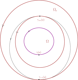
Figure 2. Circle of radius $r$ centered at $\gamma(s)$ is tangent to the boundary curves at $\gamma_{+r}(s)$ and $\gamma_{-r}(s)$

In the sequel we need the formulas calculating the Larmor centers in the Spherical and Hyperbolic geometries. For the case of the standard unite sphere in $\mathbf{R}^{3}$ we choose positive normal at $x$ to be $x$ and have for the Larmor center:

(3) $$\mathcal{L}(x,v)=\frac{\beta}{\sqrt{\beta^{2}+1}}x+\frac{1}{\sqrt{\beta^{2}+1}}[x,v]=\cos r\cdot x+\sin r[x,v],$$

where $[x,v]$ is just a positive unit normal vector to $v$ on $\Sigma$.

In the case of hyperboloid we choose again the positive normal to $\Sigma$ equal to $x$ and positive normal vector to $v$ on $\Sigma$ equals in this case $A[x,v]$. So in the Hyperbolic case we have the formula:

(4) $$\mathcal{L}(x,v)=\frac{\beta}{\sqrt{\beta^{2}-1}}x+\frac{1}{\sqrt{\beta^{2}-1}}A[x,v]=\cosh r\cdot x+\sinh rA[x,v].$$

Moreover, we introduce the mapping

$$\mathcal{M}:\Omega_{r}\rightarrow\Omega_{r}$$

by the following rule: Let $C_{-}$ and $C_{+}$ be two Larmor circles centered at $P_{-}$ and $P_{+}$, respectively. We define

$$\mathcal{M}(P_{-})=P_{+}\iff\ C_{-}\quad\textrm{is\ transformed \ to}\quad C_{+}$$

after billiard reflection at the boundary $\partial\Omega.$

It then follows easily that $\mathcal{M}:\Omega_{r}\rightarrow\Omega_{r}$ preserves the standard symplectic form (area form) of $\Sigma$ and thus $\Omega_{r}$ naturally becomes the phase space of the magnetic Birkhoff billiard. We shall call $\mathcal{M}$ the magnetic billiard map.

Given a polynomial integral $\Phi$ of the magnetic billiard, we define the function $F:\overline{\Omega}_{r}\rightarrow\overline{\Omega}_{r}$ by the requirement

(5) $$F\circ{\mathcal{L}}=\Phi.$$

This is a well-defined construction, since $\Phi$ is an integral of the magnetic flow, and therefore takes constant values on any Larmor circle. Moreover, since $\Phi$ is invariant under the billiard flow, $F$ is invariant under the billiard map $\mathcal{M}$:

(6) $$F\circ\mathcal{M}=F.$$

Notice that since $\Phi$ is a polynomial in $v$ of degree $N$, the function $F$ satisfies the following property: $F$ restricted to any circle of geodesic radius $r$ lying in $\Omega_{r}$ is a trigonometric polynomial of degree at most $N$. Indeed, the Larmor circle centered at $x$ is obtained when the unit tangent vector $v$ varies in $T_{x}\Sigma$. Choosing local coordinates $(\varphi,\psi)$ which are Euclidean at the point $x\in\Sigma$ we have

$$\Phi=\sum_{k+l=0}^{N}a_{kl}(x)v_{\varphi}^{k}v_{\psi}^{l},\quad v_{\varphi}=\cos t,v_{\psi}=\sin t,$$

so $F$ indeed becomes a trigonometric polynomial in $t$. The next theorem claims that in such a case $F$ is a restriction to $\Sigma$ of a polynomial function in $\mathbf{R}^{3}$. This theorem holds true both for Spherical and Hyperbolic case.

Theorem 3.1.

Let $\Omega_{r}$ be a domain in $\Sigma$ which is the union of all circles of radius $r$ whose centers run over a domain $\Omega$. Let $F:\overline{\Omega}_{r}\rightarrow\mathbf{R}$ be a continuous function such that the restriction of $F$ to any circle of radius $r$ of $\Omega_{r}$ is a trigonometric polynomial of degree at most $N.$ Then $F$ coincides with a restriction to $\Sigma$ of a polynomial function $\hat{F}$ in $(x_{1},x_{2},x_{3})$ of degree at most $N.$

We shall prove this theorem below in Section 9.

Moreover, we will prove the following consequence of Theorem 3.1 which enables one to apply algebraic geometry methods:

Proposition 3.2.

Suppose that the magnetic billiard in $\Omega$ admits a polynomial integral $\Phi$ and let $\hat{F}$ be the corresponding polynomial. Then

$$\hat{F}|_{\gamma_{\pm r}}={\rm const}.$$

Corollary 3.3.

If magnetic billiard in $\Omega$ has integral $\Phi$ which is linear in velocities, then $\Omega$ is a round disc on $\Sigma$.

Proof.

Indeed, by Theorem 3.1 $\hat{F}$ also has degree 1 and therefore by Proposition 3.2 the closed curves $\gamma_{\pm r}$ are intersections of $\Sigma$ with 2-planes, thus circles. Hence also $\gamma$ is a circle. ∎

In view of the Corollary 3.3 we shall assume everywhere below that the degree $N>1$.

Remark 3.4.

One can assume that the polynomial $\hat{F}$ is such that the ${\rm constant}$ in Proposition 3.2 is $0,$ for both parallel curves $\gamma_{\pm r}$. Indeed, if $\hat{F}|_{\gamma_{-r}}=c_{1}$ and $\hat{F}|_{\gamma_{+r}}=c_{2},$ one can replace $\hat{F}$ by $\hat{F}^{2}-(c_{1}+c_{2})\hat{F}+c_{1}\cdot c_{2}$ to annihilate both constants $c_{1},c_{2}.$

Since the curves $\gamma_{\pm r}$ lie in $\{\hat{F}=0\}\cap\{\Lambda-1=0\}$ we have:

Corollary 3.5.

The curves ${\gamma}_{\pm r}$ and hence also ${\gamma}$ determine irreducible algebraic sets denoted by $\hat{\gamma}_{\pm r}$ and $\hat{\gamma}$ in $\mathbf{C}^{3}$.

Next we use the folkloric fact that a curve of bidegree $(m,m)$ on a quadric is a complete intersection, i.e., intersection of the quadric with a surface of degree $m$ (we refer to [5] for more details). Moreover, using an appropriate version of Noether theorem ([22], p. 226, Chapter VIII) we can summarize the needed algebraic-geometry facts:

Theorem 3.6.

1. The ideal of irreducible algebraic sets $\hat{\gamma}_{\pm r}$ is generated by two polynomials $F_{\pm r}$ and $(\Lambda-1)$, where $F_{\pm r}$ is irreducible in the ring
   $\mathbf{C}[x_{1},x_{2},x_{3}]/{\rm mod}(\Lambda-1)$.

2. In addition we have:

   (7) $$\hat{F}=F_{\pm r}^{k}\cdot g_{\pm}\ {\rm mod}(\Lambda-1),$$

   where polynomials $g_{\pm}$ do not vanish on $\hat{\gamma}_{\pm r}$ but in finitely many points.

3. At all but finitely many points of $\hat{\gamma}_{\pm r}$ the differentials $DF_{\pm r}$ and $D\Lambda$ are not proportional, which means that the differential of the function $F_{\pm r}|_{\Sigma}$ does not vanish on $\hat{\gamma}_{\pm r}$.

In the sequel we shall use the following homogenization. Given a polynomial function on $\Sigma$ we extend it to the homogeneous function in the space away from the cone $\{\Lambda=0\}$. The extended homogeneous function we shall write with tilde. Thus for $\hat{F}=\sum_{k=0}^{N}\hat{F}_{k}$ which is a sum of homogeneous components $\hat{F}_{k}$ of degree $k$, we define

(8) $$\tilde{F}=\sum_{k=0}^{N}\hat{F}_{k}\sqrt{\Lambda}^{N-k},$$

where as above $\Lambda=(x_{1}^{2}+x_{2}^{2}+x_{3}^{2})$ for the sphere, and $\Lambda=(-x_{1}^{2}-x_{2}^{2}+x_{3}^{2})$ for the hyperboloid. Then obviously, $\tilde{F}$ is a homogeneous function of degree $N$ and

$$\tilde{F}|_{\Sigma}=\hat{F}|_{\Sigma}=F.$$

Similarly we define homogeneous functions $\tilde{F}_{\pm r}$ and $\tilde{g}_{\pm}$. So equation (7) in homogeneous form reads:

(9) $$\tilde{F}=\tilde{F}_{\pm r}^{k}\cdot\tilde{g}_{\pm}$$

Moreover from the very construction the functions

$$\tilde{F};\tilde{F}_{\pm r};\tilde{g}_{\pm}$$

all have the form

(10) $$p+q\sqrt{\Lambda},$$

where $p$, $q$ are some homogeneous polynomials with the degree of $q$ is by one less than that of $p$. Therefore we have an important:

Remark 3.7.

Function $\tilde{F}$ is analytic away from the absolute $\{\Lambda=0\}$.

3.1. Main result and example

We now turn to the formulation of our main result:

Theorem 3.8.

Let $\Omega$ be a convex bounded domain on $\Sigma$ with smooth boundary $\gamma=\partial\Omega$ which has curvature at least $\beta$ ($\beta>1$ in the Hyperbolic case). Suppose that the magnetic billiard in $\Omega$ admits a polynomial integral $\Phi.$ Then the curves $\hat{\gamma}_{\pm r}$ are smooth algebraic curves in $\mathbf{C}^{3}$.

Having this result it is easy to give a proof of Theorem 1.3 .

Proof of Theorem 1.3.

Indeed, it is easy to check that the polynomials ${F}_{\pm r}$ depend on the variable $d=\tan r$ (in the Hyperbolic case $d=\tanh r)$ in a polynomial way, so ${F}_{\pm r}$ is a polynomial in $x_{1},x_{2},x_{3}$, and $d$. Moreover, since $\gamma$ has positive curvature bounded from below by $\beta$, there is a whole open interval $r\in(\rho_{\min},\rho_{\max})$ where by Proposition 2.1 the parallel curve $\gamma_{+r}$ does have real singularities. Hence, the system of equations

$$\partial_{x_{1}}\tilde{F}_{+r}=\partial_{x_{2}}\tilde{F}_{+r}=\partial_{x_{3}}\tilde{F}_{+r}=\tilde{F}_{+r}=\Lambda-1=0$$

defines an algebraic set in ${\mathbf{C}}^{4}$ and its projection on the $d$-coordinate line is a Zariski open set. It then follows that singularities persist for all but finitely many $d.$ ∎

Example. Let $\Omega$ be the interior of the ellipse on the sphere, i.e. the intersection of the sphere with a quadratic cone

$$\partial\Omega=\left\{\frac{x_{1}^{2}}{a^{2}}+\frac{x_{2}^{2}}{b^{2}}=x_{3}^{2}\right\},\quad 0<b<a.$$

The equation of parallel curves for the ellipse is defined by the polynomial $\hat{F}$ of degree eight (see Appendix). The curve $\{\hat{F}=0\}$ on the sphere is singular for arbitrary $a$ and $b$. For $a=2,b=1$ we have

$$\hat{F}=((d^{2}-4)^{2}-10(4+5d^{2}+d^{4})x_{1}^{2}+25(1+d^{2})^{2}x_{1}^{4})(5x_{1}^{2}+d^{2}(3+5x_{1}^{2})-3)^{2}+$$

$$4(1+d^{2})(5(1+d^{2})(124+70d^{2}+31d^{4})x_{1}^{2}-3(32+60d^{2}-45d^{4}+7d^{6})-375(1+d^{2})^{2}\times$$

$$(3+d^{2})x_{1}^{4}+625(1+d^{2})^{3}x_{1}^{6})x_{2}^{2}+4(1+d^{2})^{2}(73d^{4}-248d^{2}-32-150(4+7d^{2}+3d^{4})x_{1}^{2}+$$

$$825(1+d^{2})^{2}x_{1}^{4})x_{2}^{4}+64(1+d^{2})^{3}(8-7d^{2}+25(1+d^{2})x_{1}^{2})x_{2}^{6}+256(1+d^{2})^{4}x_{2}^{8}.$$

By direct calculation we checked that the curve $\{\hat{F}=0\}$ is irreducible in the ring $\mathbf{C}[x_{1},x_{2},x_{3}]/{\rm mod}(\Lambda-1)$. Hence, by Theorem 3.8 the magnetic billiard inside the ellipse is algebraically non-integrable for any magnitude of the magnetic field. It is plausible that the curve $\hat{F}=0$ is irreducible for arbitrary $a$ and $b$.

4. Proof of the main theorem

The main step in the proof of main Theorem 3.8 is the following result. We stick to notations of Section 3.

Theorem 4.1.

Let $\tilde{F}$ be a homogeneous function of degree $N$ which coincides with $F$ on $\Sigma$. Assume $\nabla\tilde{F}$ does not vanish on $\gamma_{\pm r}$ except for finitely many points. Then the identity

(11) $$\frac{\rm Hess\ \tilde{F}}{(N-1)^{2}}\mp\beta|\nabla\tilde{F}|^{3}=\operatorname{const}$$

holds true for all points on the curve $\gamma_{\pm r}$.

Moreover the constant in the RHS of (11) is not zero.

We shall prove Theorem 4.1 in Section 7. Now we are in position to complete the proof of the main Theorem 3.8.

Proof of Theorem 3.8.

In order to fulfill the assumption of Theorem 4.1 we need to pass from $\tilde{F}$ to $\tilde{F}^{\frac{1}{k}}$ and use equation (9). Notice that $\tilde{F}^{\frac{1}{k}}$ is also conserved by the map $\mathcal{M}$. In the proof we consider the curve $\gamma_{+r}$ (the proof for the curve $\gamma_{-r}$ is identical). It then follows from Theorem 3.6 that we can write

$$\tilde{F}=\tilde{F}_{+r}^{k}\cdot\tilde{g}_{+},$$

for some integer $k\geq 1$, so that $\nabla\tilde{F}_{+r}$ and $\tilde{g}_{+}$ do not vanish on $\gamma_{+r}$ except for finitely many points. Let us take some arc $\delta$ of $\gamma_{+r}$ with this property. We may assume that $\tilde{g}_{+}$ is positive on $\delta$ (otherwise we change the signs). Therefore the equation (11) can be derived in the same manner for the function

$$\tilde{F}^{\frac{1}{k}}=\tilde{F}_{+r}\cdot\tilde{g}_{+}^{\frac{1}{k}},$$

for all points of the arc $\delta$. This function is homogeneous of degree

$$p=N/k>1.$$

Thus we have instead of (11):

(12) $$\frac{1}{(p-1)^{2}}{\rm Hess}(\tilde{F}_{+r}\cdot\tilde{g}_{+}^{\frac{1}{k}})+\beta|\nabla(\tilde{F}_{+r}\cdot\tilde{g}_{+}^{\frac{1}{k}})|^{3}={\rm const},\quad(x_{1},x_{2},x_{3})\in\delta.$$

Moreover the constant on the RHS of (12) is not zero, by Theorem 4.1. Using the identities

$${\rm Hess}(\tilde{F}_{+r}\cdot\tilde{g}_{+}^{\frac{1}{k}})=\tilde{g}_{+}^{\frac{3}{k}}{\rm Hess}(\tilde{F}_{+r}),\quad\nabla(\tilde{F}_{+r}\cdot\tilde{g}_{+}^{\frac{1}{k}})=\tilde{g}_{+}^{\frac{1}{k}}\nabla(\tilde{F}_{+r}),$$

which are valid for all $(x_{1},x_{2},x_{3})\in\{\tilde{F}_{+r}=0\}$, we obtain from (12) that

(13) $$\tilde{g}_{+}^{\frac{3}{k}}\left({\frac{1}{(p-1)^{2}}\rm Hess}(\tilde{F}_{+r})+\beta|\nabla\tilde{F}_{+r}|^{3}\right)={\rm const},\quad(x_{1},x_{2},x_{3})\in\delta.$$

Raising back to the power $k$ we get

(14) $$\tilde{g}_{+}^{{3}}\left({\frac{1}{(p-1)^{2}}\rm Hess}(\tilde{F}_{+r})+\beta|\nabla\tilde{F}_{+r}|^{3}\right)^{k}={\rm const},\ (x_{1},x_{2},x_{3})\in\delta.$$

Let us prove now, that the curve $\hat{\gamma}_{+r}$ is non-singular in $\mathbf{C}^{3}$. We argue by contradiction. Suppose, there exist a singular point $P$ of $\hat{\gamma}_{+r}\subset\{\Lambda-1=0\}\subset\mathbf{C}^{3}$. Pick any point $Q\in\delta$, and consider a path $\alpha$ on the algebraic curve $\hat{\gamma}_{+r}$ going from $Q$ to $P$ avoiding the singular points of $\tilde{F}_{+r}$. Using the particular form of $\tilde{F}_{+r}$ and $\tilde{g}_{+}$ given by Theorem 3.5 we see that the equation (14) remains valid for analytic continuation of the functions $\tilde{F}_{+r}$, $\tilde{g}_{+}$ along the path $\alpha$. Hence it remains valid also at the point $P$. But this is impossible, because the LHS is zero at $P$ while the constant is not zero at the RHS. The proof is completed. ∎

5. Boundary values of the integral.

In this Section we prove Proposition 3.2.

Take a point $x$ on $\gamma$. Let $v$ be a positive unit tangent vector to $\gamma$. Let $C_{-}$ and $C_{+}$ be the incoming and outgoing circles with the unit tangent vectors $v_{-}$ and $v_{+}$ at the impact point $x$. We are interested in the two cases when the reflection angle between $v$ and $v_{-}$ is close to $0$ or to $\pi$. These two possibilities correspond to the following cases:

(15) $$(a)\quad\quad v_{-}=R_{-\varepsilon}v,\quad\ \quad v_{+}=R_{\varepsilon}v,$$

$$(b)\quad v_{-}=R_{\varepsilon}(-v),\quad v_{+}=R_{-\varepsilon}(-v),$$

where $R_{\varepsilon}$ is the counterclockwise rotation of the tangent plane $T_{x}\Sigma$ by a small angle $\varepsilon$, see Fig. 3.

We define

$$P_{-}(\varepsilon)={\mathcal{L}}(x,v_{-})=\exp_{x}(rJ(v_{-})),\quad P_{+}(\varepsilon)={\mathcal{L}}(x,v_{+})=\exp_{x}(rJ(v_{+})).$$

In the case (a) we have

(16) $$P_{-}(\varepsilon)=\exp_{x}(rJ(R_{-\varepsilon}v)),\quad P_{+}(\varepsilon)=\exp_{x}(rJ(R_{\varepsilon}v)).$$

In the case (b),

(17) $$P_{-}(\varepsilon)=\exp_{x}(-rJ(R_{\varepsilon}v)),\quad P_{+}(\varepsilon)=\exp_{x}(-rJ(R_{-\varepsilon}v)).$$

We write:

$$P_{-}:=P_{-}(\varepsilon),\ P_{+}:=P_{+}(\varepsilon),P_{0}:=P_{-}(0)=P_{+}(0).$$

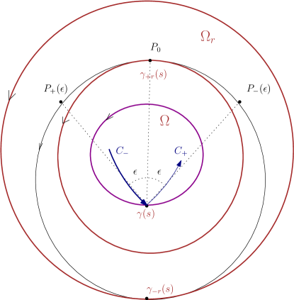
Figure 3. The center $P_{-}$ of the circle $C_{-}$ is mapped by $\mathcal{M}$ to the center $P_{+}$ of $C_{+}$

Notice that in case (a) the middle point of the short arc that connects the points $P_{-}(\varepsilon)$ and $P_{+}(\varepsilon)$ is $P_{0}=\exp_{x}(rJ(v))\in\gamma_{+r}$, while for the case (b) the middle point is $P_{0}=\exp_{x}(rJ(-v))\in\gamma_{-r}$.

Proof of Proposition 3.2.

The condition 2. of Definition 1.2 reads in terms of $F$

(18) $$F(P_{-}(\varepsilon))=F(P_{+}(\varepsilon)).$$

Differentiating this equality with respect to $\varepsilon$ at $\varepsilon=0$ we compute in the case (a):

$$\frac{d}{d\varepsilon}{|_{{}_{\varepsilon=0}}}F(P_{-}(\varepsilon))=dF|_{P_{0}}\left(\frac{d}{d\varepsilon}{|_{{}_{\varepsilon=0}}}P_{-}(\varepsilon)\right)=dF|_{P_{0}}(Y(r)),$$

$$\frac{d}{d\varepsilon}|_{\varepsilon=0}F(P_{+}(\varepsilon))=dF|_{P_{0}}\left(\frac{d}{d\varepsilon}{|_{{}_{\varepsilon=0}}}P_{+}(\varepsilon)\right)=dF|_{P_{0}}(-Y(r)),$$

where $Y(t)$ is an orthogonal Jacobi field along the geodesic $\exp_{x}(tJv)$ corresponding to the radial family of geodesics $\exp_{x}(tR_{\varepsilon}Jv)$. Thus $Y(r)$ is tangent to $\gamma_{+r}$ at the point $P_{0}$. The last two equalities together imply :

$$dF|_{P_{0}}(Y(r))=0,$$

so $F$ has a constant value on $\gamma_{+r}$. Analogously one treats the case (b). This completes the proof of Proposition 3.2 ∎

6. Remarkable equation

In this Section we deduce the remarkable equation expressing (6) for a function $F:\overline{\Omega}_{r}\rightarrow\overline{\Omega}_{r}$ invariant under the map $\mathcal{M}$. This equation is valid for those $F$ which have non-vanishing gradient at a point on the boundary of $\Omega_{r}$. Moreover we may assume that $n_{\pm r}=A\frac{\nabla F}{|\nabla F|}$ is a positive unite normal to $\gamma_{\pm r}$, i.e. the basis $(\dot{\gamma}_{\pm r},n_{\pm r})$ is positive (otherwise we change the sign of $F$). In order to perform computations we need to rewrite the equation (6) and hence (18) in terms of the homogeneous function $\tilde{F}$ defined by (8).

We fix a point $(x_{0},\pm v_{0}),\ v_{0}=\dot{\gamma},\ n_{0}=Jv_{0}$ and rewrite (18):

(19) $$F({\mathcal{L}}(x_{0},R_{-\varepsilon}(\pm v_{0})))=F({\mathcal{L}}(x_{0},R_{+\varepsilon}(\pm v_{0}))),$$

where the sign $+$ and $-$ correspond to the cases (a) and (b) in (15) respectively.

In what follows we develop (23) in $\varepsilon$ at $\varepsilon=0$. This will contain derivatives $\tilde{F}$ at the point $P_{0}={\mathcal{L}}(x_{0},v_{0})$ for the case (a) (at $P_{0}={\mathcal{L}}(x_{0},-v_{0})$ for the case (b)). We shall denote by $y_{0}$ the point $P_{0}$ viewed in $\mathbf{R}^{3}$. Notice that since $\gamma_{\pm r}$ are parallel curves to $\gamma$ their tangent vector at $P_{0}$ viewed in $\mathbf{R}^{3}$ is exactly $\mp v_{0}$. Moreover it follows from Euler formula for $\tilde{F}$ that the positive unite normal to $\gamma_{\pm r}$ at $P_{0}$ as a vector of $\mathbf{R}^{3}$ equals

$$n_{\pm r}(y_{0})=A\frac{\nabla\tilde{F}}{|\nabla\tilde{F}|}\left(y_{0}\right).$$

In addition,

(20) $$v_{0}=-A\frac{[y_{0},A\nabla\tilde{F}]}{|\nabla\tilde{F}|}\left(y_{0}\right).$$

One more thing we need is to rewrite positive normal vector $n_{0}$ to $\gamma$ at $x_{0}$ via $\tilde{F}$ at the point $y_{0}$. This can be done as follows. Vectors $n_{0}$ and $n_{\pm r}$ are unite vectors which are tangent (with opposite orientation) to the same geodesic $\exp_{x_{0}}(tJv_{0})$ at the points which are at distance $r$ apart. Then we compute in the spherical case:

(21) $$n_{0}=\pm(-\cos r\cdot n_{\pm r}(y_{0})+\sin r\cdot y_{0})=\pm(-\cos r\cdot\frac{\nabla\tilde{F}}{|\nabla\tilde{F}|}\left(y_{0}\right)+\sin r\cdot y_{0}).$$

In the hyperbolic case this formula reads:

(22) $$n_{0}=\pm(-\cosh r\cdot n_{\pm r}(y_{0})-\sinh r\cdot y_{0})=\pm(-\cosh r\cdot A\frac{\nabla\tilde{F}}{|\nabla\tilde{F}|}\left(y_{0}\right)-\sinh r\cdot y_{0}).$$

Now we shall substitute into (19) the expression

$$R_{\varepsilon}(\pm v_{0})=\cos\varepsilon(\pm v_{0})+\sin\varepsilon(\pm n_{0})$$

together with the explicit formulas (20), (21), (22).

We shall consider the cases of sphere and hyperboloid separately.

Case 1. In the case of sphere we get by the substitution the RHS of (19) :

(23) $$F({\mathcal{L}}(x_{0},R_{+\varepsilon}(\pm v_{0})))=\tilde{F}\left(\cos rx_{0}+\sin r[x_{0},R_{\varepsilon}(\pm v_{0})]\right)=$$

$$=\tilde{F}\left(\cos rx_{0}+\sin r[x_{0},(\cos\varepsilon(\pm v_{0})+\sin\varepsilon(\pm n_{0}))]\right)=$$

$$=\tilde{F}\left(y_{0}+\sin r\bigl{(}\cos{\varepsilon}-1)[x_{0},(\pm v_{0})]+\sin r\sin\varepsilon[x_{0},(\pm n_{0})]\right)=$$

$$=\tilde{F}\left(y_{0}\pm\sin r\bigl{(}\cos{\varepsilon}-1)n_{0}\mp\sin r\sin\varepsilon v_{0}\right)=$$

$$=\tilde{F}\left(y_{0}+\sin r\bigl{(}\cos{\varepsilon}-1)\left(-\cos r\cdot\frac{\nabla\tilde{F}}{|\nabla\tilde{F}|}\left(y_{0}\right)+\sin r\cdot y_{0}\right)\pm\right.$$

$$\left.\sin r\sin\varepsilon\frac{[y_{0},\nabla\tilde{F}]}{|\nabla\tilde{F}|}\left(y_{0}\right)\right).$$

So finally we can rewrite equation (19) as

(24) $$\tilde{F}\left(y_{0}+\sin r\bigl{(}\cos{\varepsilon}-1)\left(-\cos r\cdot\frac{\nabla\tilde{F}}{|\nabla\tilde{F}|}\left(y_{0}\right)+\sin r\cdot y_{0}\right)\mp\right.$$

$$\left.\sin r\sin\varepsilon\frac{[y_{0},\nabla\tilde{F}]}{|\nabla\tilde{F}|}\left(y_{0}\right)\right)$$

$$=\tilde{F}\left(y_{0}+\sin r\bigl{(}\cos{\varepsilon}-1)\left(-\cos r\cdot\frac{\nabla\tilde{F}}{|\nabla\tilde{F}|}\left(y_{0}\right)+\sin r\cdot y_{0}\right)\pm\right.$$

$$\left.\sin r\sin\varepsilon\frac{[y_{0},\nabla\tilde{F}]}{|\nabla\tilde{F}|}\left(y_{0}\right)\right).$$

Case 2. In the hyperbolic case formulas are similar:

(25) $$F({\mathcal{L}}(x_{0},R_{+\varepsilon}(\pm v_{0})))=\tilde{F}\left(\cosh rx_{0}+\sinh rA[x_{0},R_{\varepsilon}(\pm v_{0})]\right)=$$

$$=\tilde{F}\left(\cosh rx_{0}+\sinh rA[x_{0},(\cos\varepsilon(\pm v_{0})+\sin\varepsilon(\pm n_{0}))]\right)=$$

$$=\tilde{F}\left(y_{0}+\sinh r\bigl{(}\cos{\varepsilon}-1)A[x_{0},(\pm v_{0})]+\sinh r\sin\varepsilon A[x_{0},(\pm n_{0})]\right)=$$

$$=\tilde{F}\left(y_{0}\pm\sinh r\bigl{(}\cos{\varepsilon}-1)n_{0}\mp\sinh r\sin\varepsilon v_{0}\right)=$$

$$=\tilde{F}\left(y_{0}-\sinh r\bigl{(}\cos{\varepsilon}-1)\left(\sinh r\cdot y_{0}+\cosh r\cdot A\frac{\nabla\tilde{F}}{|\nabla\tilde{F}|}\left(y_{0}\right)\right)\pm\right.$$

$$\left.\sinh r\sin\varepsilon A\frac{[y_{0},A\nabla\tilde{F}]}{|\nabla\tilde{F}|}\left(y_{0}\right)\right).$$

Thus in the hyperbolic case we get finally:

(26) $$\tilde{F}\left(y_{0}-\sinh r\bigl{(}\cos{\varepsilon}-1)\left(\sinh r\cdot y_{0}+\cosh r\cdot A\frac{\nabla\tilde{F}}{|\nabla\tilde{F}|}\left(y_{0}\right)\right)\mp\right.$$

$$\left.\sinh r\sin\varepsilon A\frac{[y_{0},A\nabla\tilde{F}]}{|\nabla\tilde{F}|}\left(y_{0}\right)\right)=$$

$$=\tilde{F}\left(y_{0}-\sinh r\bigl{(}\cos{\varepsilon}-1)\left(\sinh r\cdot y_{0}+\cosh r\cdot A\frac{\nabla\tilde{F}}{|\nabla\tilde{F}|}\left(y_{0}\right)\right)\pm\right.$$

$$\left.\sinh r\sin\varepsilon A\frac{[y_{0},A\nabla\tilde{F}]}{|\nabla\tilde{F}|}\left(y_{0}\right)\right).$$

7. Terms of $\varepsilon^{3}$ and proof of Theorem 4.1.

In this Section we compute and put in a very compact form terms of order $\varepsilon^{3}$ of equations (24), (26). Then we prove Theorem 4.1.

In order to write the terms of order $\varepsilon^{3}$ of the equations (24), (26) we first rewrite the argument of (24):

(27) $$y_{0}+\sin r\bigl{(}\cos{\varepsilon}-1)\left(-\cos r\cdot\frac{\nabla\tilde{F}}{|\nabla\tilde{F}|}\left(y_{0}\right)+\sin r\cdot y_{0}\right)\mp\sin r\sin\varepsilon\frac{[y_{0},\nabla\tilde{F}]}{|\nabla\tilde{F}|}\left(y_{0}\right)=$$

$$\left.=y_{0}(1-2\sin^{2}r\sin^{2}(\varepsilon/2))+2\sin r\cos r\sin^{2}(\varepsilon/2)\frac{\nabla\tilde{F}}{|\nabla\tilde{F}|}(y_{0})\mp\right.$$

$$\sin r\sin\varepsilon\frac{[y_{0},\nabla\tilde{F}]}{|\nabla\tilde{F}|}\left(y_{0}\right)=$$

$$(1-2\sin^{2}r\sin^{2}(\varepsilon/2))\left(y_{0}+\frac{\nabla\tilde{F}}{|\nabla\tilde{F}|}\frac{2\sin r\cos r\sin^{2}(\varepsilon/2)}{1-2\sin^{2}r\sin^{2}(\varepsilon/2)}\mp\right.$$

$$\left.\frac{\sin r\sin\varepsilon}{1-2\sin^{2}r\sin^{2}(\varepsilon/2)}\frac{[y_{0},\nabla\tilde{F}]}{|\nabla\tilde{F}|}\right).$$

We can neglect the factor in front of the brackets, since the function $\tilde{F}$ is homogeneous. So up to order $\varepsilon^{3}$ we have for the argument :

$$y_{0}+\frac{\sin r\cos r}{2}\varepsilon^{2}\frac{\nabla\tilde{F}}{|\nabla\tilde{F}|}\mp\left(\sin r\varepsilon+\left(\frac{1}{2}\sin^{3}r-\frac{1}{6}\sin r\right)\varepsilon^{3}\right)\cdot\frac{[y_{0},\nabla\tilde{F}]}{|\nabla\tilde{F}|}.$$

Using this one can write the third order expansion for (24) and analogously for (26). It turns out that the terms of order $\varepsilon^{3}$ in the equations (24), (26) can be organized so that they are complete derivatives along the tangent vector $v$ to the curves $\gamma_{\pm r}$ (it is given through $F$ by formula(20)). On the Sphere this reads:

(28) $$L_{v}\left(\frac{\rm Hess\ \tilde{F}}{(N-1)^{2}}\mp\cot r|\nabla\tilde{F}|^{3}\right)=0.$$

As for the Hyperbolic case:

(29) $$L_{v}\left(\frac{\rm Hess\ \tilde{F}}{(N-1)^{2}}\mp\coth r|\nabla\tilde{F}|^{3}\right)=0.$$

So in both cases we can write (28) and (29) as

(30) $$L_{v}\left(\frac{\rm Hess\ \tilde{F}}{(N-1)^{2}}\mp\beta|\nabla\tilde{F}|^{3}\right)=0.$$

Now we are in position to prove Theorem 4.1.

Proof of Theorem 4.1.

The identity (11) follows from (30). We need to show that the constant in the RHS of (30) is not zero. For the proof we need the following important formula for the geodesic curvature of curves on $\Sigma$ which we prove in Section 8.

Lemma 7.1.

Let $\tilde{F}$ be a homogeneous function in $\mathbf{R}^{3}$ of degree $N>1$. The geodesic curvature of the curve $\{\tilde{F}=0\}$ on $\Sigma$ (with respect to the normal $A\frac{\nabla\tilde{F}}{|\nabla\tilde{F}|}$) at a non-singular point is given in both geometries by the same formula:

(31) $$k=\frac{\rm Hess\ \tilde{F}}{(N-1)^{2}|\nabla\tilde{F}|^{3}}.$$

We prove the Lemma in Section 8.

It follows from Lemma 7.1 that if the constant in (11) is zero then the geodesic curvature of the curve $\gamma_{\pm r}$ equals $\pm\beta$. But this cannot happen due to the inequality of Proposition 2.3. This completes the proof of Theorem 4.1. ∎

8. Geodesic curvature in homogeneous coordinates.

Proof of Lemma 7.1.

Set positive normal and the tangent vector to the curve at the point $x$:

(32) $$n=A\frac{\nabla\tilde{F}}{|\nabla\tilde{F}|},\quad v=-A\frac{[x,A\nabla\tilde{F}]}{|\nabla\tilde{F}|}.$$

Then we use the formula for geodesic curvature on $\Sigma$ using Frenet formula:

$$k=-<\nabla_{v}n,Av>,$$

where $\nabla$ is the standard flat connection on $\mathbf{R}^{3}$.

$$k=-\left<\nabla_{v}\left(A\frac{\nabla\tilde{F}}{|\nabla\tilde{F}|}\right),Av\right>=-\frac{1}{|\nabla\tilde{F}|}<\nabla_{v}\nabla\tilde{F},v>=-\frac{1}{|\nabla\tilde{F}|}<Hv,v>,$$

where $H$ denotes the matrix of second derivatives of $\tilde{F}$. Notice that we omitted another term containing the derivative of $\frac{1}{|\nabla\tilde{F}|}$ using the fact that $<A\nabla\tilde{F},Av>=0$. Next we use Euler identities for the derivatives of $\tilde{F}$:

(33) $$Hx=(N-1)\nabla\tilde{F}.$$

Thus we continue using (32), (33):

$$k=-\frac{1}{|\nabla\tilde{F}|^{3}}<H[Ax,\nabla\tilde{F}],[Ax,\nabla\tilde{F}]>=$$

$$=-\frac{1}{(N-1)^{2}|\nabla\tilde{F}|^{3}}<H[Ax,Hx],[Ax,Hx]>=$$

$$=-\frac{{\rm Hess}\tilde{F}}{(N-1)^{2}|\nabla\tilde{F}|^{3}}<[Ax,Hx],[H^{-1}Ax,x]>=$$

$$=-\frac{{\rm Hess}\tilde{F}}{(N-1)^{2}|\nabla\tilde{F}|^{3}}\left(<Ax,H^{-1}Ax><Hx,x>-<Ax,x><Hx,H^{-1}Ax>\right),$$

where ${\rm Hess}\tilde{F}$ is the determinant of $H$.

At last we notice that

$$<Hx,x>=(N-1)<\nabla\tilde{F},x>=(N-1)N\cdot\tilde{F}(x)=0,$$

by Euler identity. Thus we get

$$k=\frac{{\rm Hess}\tilde{F}}{(N-1)^{2}|\nabla\tilde{F}|^{3}}<Ax,x>^{2}=\frac{{\rm Hess}\tilde{F}}{(N-1)^{2}|\nabla\tilde{F}|^{3}},$$

which yields (31). ∎

9. Proof of Theorem 3.1

In the proof we follow our strategy from [10].

Proof.

Let us assume first that $F$ is a $C^{\infty}$-function. We shall say that $F$ has property $P_{N}$ if the restriction of $F$ to any circle of radius $r$ lying in $\Omega_{r}$ is a trigonometric polynomial of degree at most $N$. The proof of Theorem 3.1 goes by induction on the degree $N$.

1) For $N=0$, the lemma obviously holds, since if $F$ has property $P_{0}$, then $F$ is a constant on any circle of radius $r$ and hence must be a constant on the whole $\Omega_{r}$, because any two points of $\Omega_{r}$ can be connected by a union of a finite number of circular arcs of radius $r$.

2) Assume now that any function satisfying property $P_{N-1}$ is a restriction to $\Sigma$ of a polynomial function in $(x_{1},x_{2},x_{3})$ of degree at most $N-1.$

Let $F$ be any smooth function on $\Omega_{r}$ with property $P_{N}$. Fix a point $x_{*}\in\Omega$ and consider the circle $C_{0}$ of radius $r$ centered in $x_{*}$. Applying an appropriate isometry of $\Sigma$ we may assume that

$$x_{*}=(0,0,1)\in\mathbf{R}^{3}\quad{\rm and}\quad C_{0}=\{x_{3}=h\},$$

where $h=\cos r$ in the spherical case and $h=\cosh r$ for hyperboloid. Obviously there exists a polynomial $\hat{F}_{0}$ in $(x_{1},x_{2},x_{3})$ of degree at most $N$ such that satisfying ${F}|_{C_{0}}=\hat{F}_{0}|_{C_{0}}.$ Then applying Hadamard’s lemma to the function $F-\hat{F}_{0}$ one can find a $C^{\infty}$ function $G:\Omega_{r}\rightarrow\mathbf{R}$ such that

(34) $$F(x)-\hat{F_{0}}(x)=(x_{3}-h)G(x),\quad\forall x\in\Omega_{r}.$$

Let us show now that $G$ has property $P_{N-1}$. Then by induction we will have that $G$ is a restriction to $\Sigma$ of a polynomial $\hat{G}$ of degree $(N-1)$ and thus by (34), $F$ is a polynomial of degree at most $N$. Thus we need to show that the function $g:=G|_{C}$ is a trigonometric polynomial of degree at most $N-1$, for any circle $C$ of radius $r$ lying in $\Omega_{r}$. We can apply suitable rotation along the $x_{3}$-axes so that the center of $C$ has $x_{1}=0$. Let us denote by $\alpha$ the geodesic distance between the centers of $C_{0}$ and $C$ in $\Omega$.

We shall split the proof in two cases.

Case 1. If $\Sigma$ is the sphere, we can write $C$ as follows

$$C=R_{\alpha}C_{0},\quad R_{\alpha}=\begin{pmatrix}1&0&0\\ 0&\cos\alpha&-\sin\alpha\\ 0&\sin\alpha&\cos\alpha\end{pmatrix}.$$

Therefore parametrizing $C_{0}$ we compute the parametrization of $C$ as follows

$$C_{0}=(\sin r\sin t,\sin r\cos t,\cos r)\Rightarrow C=(*,*,\ \sin r\cos t\sin\alpha+\cos\alpha\cos r).$$

Then we compute $(x_{3}-h)|_{C}$:

(35) $$(x_{3}-h)|_{C}=\sin r\cos t\sin\alpha+\cos\alpha\cos r-\cos r=$$

$$=\sin r\sin\alpha\left(\frac{e^{it}+e^{-it}}{2}\right)-\cos r(1-\cos\alpha).$$

Substituting (35) into (34) we get

$$(F-\hat{F}_{0})|_{C}=(\sin r\sin\alpha\left(\frac{e^{it}+e^{-it}}{2}\right)-\cos r(1-\cos\alpha))\cdot G|_{C}.$$

Expanding the left- and the right-hand sides in Fourier series we get

$$\sum_{-\infty}^{+\infty}f_{k}e^{ikt}=(\sin r\sin\alpha\left(\frac{e^{it}+e^{-it}}{2}\right)-\cos r(1-\cos\alpha))\sum_{-\infty}^{+\infty}g_{k}e^{ikt},$$

where $f_{k}$ are Fourier coefficients of $(F-\hat{F}_{0})|_{C}$. Moreover, we have

$$f_{k}=0,\quad|k|>N,$$

since both $F$ and $\hat{F}_{0}$ have property $P_{N}.$ Thus we obtain a linear recurrence relation for the coefficients $g_{k}$:

$$\sin\alpha\sin r\cdot g_{k+1}-4\cos r\sin^{2}(\alpha/2)\cdot g_{k}+\sin\alpha\sin r\cdot g_{k-1}=0,\quad|k|>N.$$

The characteristic polynomial of this difference equation,

$$\lambda^{2}-2\cot r\tan(\alpha/2)\lambda+1=0,$$

has the discriminant

$$D=\cot^{2}r\tan^{2}(\alpha/2)-1$$

which is strictly negative due to the inequality $\alpha/2<r$, which holds true for the following reason: the inequality of our setup, $\cot r=\beta<k$ implies that the distance between any two points of $\Omega$ is less than $2r$, in particular $\alpha<2r$. Therefore the characteristic equation has two complex conjugate roots $\lambda_{1,2}=e^{\pm i\varphi}$ and therefore we can write

$$g_{N+l}=c_{1}e^{il\varphi}+c_{2}e^{-il\varphi},\quad l\geq 2,$$

where

$$c_{1}+c_{2}=g_{N},\quad c_{1}e^{i\varphi}+c_{2}e^{-i\varphi}=g_{N+1}.$$

It is obvious now that if at least one of the coefficients $g_{N}$ or $g_{N+1}$ does not vanish, then at least one of the constants $c_{1},c_{2}$ does not vanish, and therefore the sequence $\{g_{N+l}\}$ does not converge to $0$ when $l\rightarrow+\infty$. This contradicts the continuity of $g$. Therefore, both $g_{N}$ and $g_{N+1}$ must vanish, and so $g$ is a trigonometric polynomial of degree at most $N-1$, proving that $G$ has property $P_{N-1}$. This completes the proof of Theorem 3.1 for $C^{\infty}$-case for the sphere.

Case 2. If $\Sigma$ is the upper sheet of the hyperboloid, we can write $C$ as follows

$$C=Rh_{\alpha}C_{0},\quad Rh_{\alpha}=\begin{pmatrix}1&0&0\\ 0&\cosh\alpha&\sinh\alpha\\ 0&\sinh\alpha&\cosh\alpha\end{pmatrix}.$$

Therefore parametrizing $C_{0}$ we compute the parametrization of $C$ as follows

$$C_{0}=(\sinh r\sin t,\sinh r\cos t,\cosh r)\Rightarrow C=(*,*,\ \sinh r\cos t\sinh\alpha+\cosh\alpha\cosh r).$$

Then we compute $(x_{3}-h)|_{C}$:

(36) $$(x_{3}-h)|_{C}=\sinh r\cos t\sinh\alpha+\cosh\alpha\cosh r-\cosh r=$$

$$=\sinh r\sinh\alpha\left(\frac{e^{it}+e^{-it}}{2}\right)-\cosh r(1-\cosh\alpha).$$

Substituting (36) into (34) we get

$$(F-\hat{F}_{0})|_{C}=(\sinh r\sinh\alpha\left(\frac{e^{it}+e^{-it}}{2}\right)-\cosh r(1-\cosh\alpha))\cdot G|_{C}.$$

Expanding again the left- and the right-hand sides in Fourier series we get

$$\sum_{-\infty}^{+\infty}f_{k}e^{ikt}=(\sinh r\sinh\alpha\left(\frac{e^{it}+e^{-it}}{2}\right)-\cosh r(1-\cosh\alpha))\sum_{-\infty}^{+\infty}g_{k}e^{ikt},$$

where $f_{k}$ are Fourier coefficients of $(F-\hat{F}_{0})|_{C}$. Moreover, we have

$$f_{k}=0,\quad|k|>N,$$

since both $F$ and $\hat{F}_{0}$ have property $P_{N}.$ Thus the linear recurrence relation in Case 2 reads:

$$\sinh\alpha\sinh r\cdot g_{k+1}-4\cosh r\sinh^{2}(\alpha/2)\cdot g_{k}+\sinh\alpha\sinh r\cdot g_{k-1}=0,\quad|k|>N.$$

The characteristic polynomial of this difference equation,

$$\lambda^{2}-2\coth r\cdot\tanh(\alpha/2)\lambda+1=0,$$

has the discriminant

$$D=\coth^{2}r\cdot\tanh^{2}(\alpha/2)-1$$

which is again strictly negative due to the inequality $\alpha/2<r$ as in the previous case. Therefore the characteristic equation has two complex conjugate roots and we finish exactly as in the Case 1. This completes the proof of Theorem 3.1 for $C^{\infty}$-case for the hyperboloid.

The general case when $F$ is only continuous, can be proven by a limiting argument exactly as we did in [10]. We omit the details. ∎

10. Appendix

Let $\Omega$ be the interior of the ellipse on the sphere, i.e. the intersection of the sphere with a quadratic cone

$$\partial\Omega=\left\{\frac{x_{1}^{2}}{a^{2}}+\frac{x_{2}^{2}}{b^{2}}=x_{3}^{2}\right\},\quad 0<b<a.$$

The equation of the parallel curves for an ellipse reads $\hat{F}=0$, where

$$\hat{F}=(a^{4}(x_{2}^{2}+d^{2}(x_{2}^{2}-1))^{2}((1+a^{2})^{2}(1+d^{2})^{2}x_{1}^{4}+2(1+a^{2})(1+d^{2})x_{1}^{2}\times$$

$$(x_{2}^{2}-a^{2}+d^{2}(x_{2}^{2}-1))+(a^{2}+x_{2}^{2}+d^{2}(x_{2}^{2}-1))^{2})+2a^{2}b^{2}(a^{6}((1+d^{2})^{2}x_{2}^{4}-d^{2}-$$

$$(1+d^{2})^{2}x_{2}^{2})-(1+a^{2})^{2}(1+d^{2})^{2}x_{1}^{4}(3d^{2}(a^{2}+d^{2})+(1+d^{2})(a^{2}(3+d^{2})-d^{2})x_{2}^{2}-$$

$$(2+a^{2})(1+d^{2})^{2}x_{2}^{4})+a^{4}(d^{4}+d^{2}(2+5d^{2}+3d^{4})x_{2}^{2}-3(1+d^{2})^{2}(1+2d^{2})x_{2}^{4}+$$

$$3(1+d^{2})^{3}x_{2}^{6})+(1+a^{2})(1+d^{2})x_{1}^{2}(3a^{4}d^{2}+2a^{2}d^{4}+3d^{6}+(1+d^{2})(3a^{2}d^{2}(d^{2}-1)-$$

$$5d^{4}+a^{4}(3+2d^{2}))x_{2}^{2}-(1+d^{2})^{2}(2a^{4}-d^{2}+a^{2}(6d^{2}-1))x_{2}^{4}+(1+3a^{2})(1+d^{2})^{3}x_{2}^{6})+$$

$$a^{2}(d^{2}-2(1+d^{2})^{2}x_{2}^{2}+2(1+d^{2})^{2}x_{2}^{4})(x_{2}^{2}+d^{2}(x_{2}^{2}-1))^{2}+d^{2}(x_{2}^{2}+d^{2}(x_{2}^{2}-1))^{3}+$$

$$(1+a^{2})^{3}(1+d^{2})^{3}x_{1}^{6}(x_{2}^{2}+d^{2}(1+x_{2}^{2})))+b^{8}((1+d^{2})x_{2}^{2}-1)^{2}((1+a^{2})^{2}(1+d^{2})^{2}x_{1}^{4}+$$

$$2(1+a^{2})(1+d^{2})x_{1}^{2}(a^{2}((1+d^{2})x_{2}^{2}-1)-d^{2})+(d^{2}+a^{2}((1+d^{2})x_{2}^{2}-1))^{2})+$$

$$b^{4}((1+a^{2})^{4}(1+d^{2})^{4}x_{1}^{8}+a^{8}((1+d^{2})x_{2}^{2}-1)^{2}+2(1+a^{2})^{3}(1+d^{2})^{3}x_{1}^{6}((1+a^{2})\times$$

$$(1+d^{2})x_{2}^{2}-2(a^{2}+d^{2}))+(1+a^{2})^{2}(1+d^{2})^{2}x_{1}^{4}(6a^{4}+10a^{2}d^{2}+6d^{4}+2(1+d^{2})\times$$

$$(a^{2}(1+d^{2})-3a^{4}-3d^{2})x_{2}^{2}+(1+8a^{2}+a^{4})(1+d^{2})^{2}x_{2}^{4})+2a^{6}(d^{2}+(3+5d^{2}+2d^{4})x_{2}^{2}-$$

$$3(1+d^{2})^{2}(2+d^{2})x_{2}^{4}+3(1+d^{2})^{3}x_{2}^{6})+2a^{2}d^{2}(d^{4}+d^{2}(2+5d^{2}+3d^{4})x_{2}^{2}-3(1+d^{2})^{2}\times$$

$$(1+2d^{2})x_{2}^{4}+3(1+d^{2})^{3}x_{2}^{6})+2a^{4}((1+d^{2})^{2}(3+10d^{2}+3d^{4})x_{2}^{4}-3d^{4}-4(d+d^{3})^{2}x_{2}^{2}-$$

$$6(1+d^{2})^{4}x_{2}^{6}+3(1+d^{2})^{4}x_{2}^{8})+d^{4}(x_{2}^{2}+d^{2}(x_{2}^{2}-1))^{2}-2(1+a^{2})(1+d^{2})x_{1}^{2}(a^{6}(2-$$

$$3(1+d^{2})x_{2}^{2}+(1+d^{2})^{2}x_{2}^{4})+d^{2}(2d^{4}-3d^{2}(1+d^{2})x_{2}^{2}+(1+d^{2})^{2}x_{2}^{4})+a^{2}(4d^{4}+d^{2}(3+$$

$$8d^{2}+5d^{4})x_{2}^{2}-(1+d^{2})^{2}(2d^{2}-3)x_{2}^{4}-3(1+d^{2})^{3}x_{2}^{6})+a^{4}(4d^{2}+(5+8d^{2}+3d^{4})x_{2}^{2}+$$

$$(1+d^{2})^{2}(3d^{2}-2)x_{2}^{4}-3(1+d^{2})^{3}x_{2}^{6})))+2b^{6}(a^{6}((1+d^{2})x_{1}^{2}-1+(1+d^{2})x_{2}^{2})^{2}\times$$

$$((1+d^{2})x_{2}^{2}-1+(1+d^{2})x_{1}^{2}(1+(1+d^{2})x_{2}^{2}))+(x_{1}^{2}+d^{2}(x_{1}^{2}-1))^{2}((1+d^{2})^{2}x_{2}^{4}-d^{2}-$$

$$(1+d^{2})^{2}x_{2}^{2}+(1+d^{2})x_{1}^{2}(1+(1+d^{2})x_{2}^{2}))+a^{2}(3(1+d^{2})^{3}x_{1}^{6}(1+(1+d^{2})x_{2}^{2})+$$

$$(1+d^{2})^{2}x_{1}^{4}(4(1+d^{2})^{2}x_{2}^{4}-(1+7d^{2}+6d^{4})x_{2}^{2}-3-6d^{2})+d^{2}(d^{2}+(3+5d^{2}+2d^{4})x_{2}^{2}-$$

$$3(1+d^{2})^{2}(2+d^{2})x_{2}^{4}+3(1+d^{2})^{3}x_{2}^{6})+(1+d^{2})x_{1}^{2}((3+2d^{2}+2d^{4}+3d^{6})x_{2}^{2}+$$

$$d^{2}(2+3d^{2})-(1+d^{2})^{2}(6+d^{2})x_{2}^{4}+3(1+d^{2})^{3}x_{2}^{6}))+a^{4}(3(1+d^{2})^{3}x_{1}^{6}(1+(1+d^{2})x_{2}^{2})+$$

$$((1+d^{2})x_{2}^{2}-1)^{2}(d^{2}-2(1+d^{2})^{2}x_{2}^{2}+2(1+d^{2})^{2}x_{2}^{4})+(1+d^{2})^{2}x_{1}^{4}((1-2d^{2}-3d^{4})x_{2}^{2}$$

$$-3(2+d^{2})+5(1+d^{2})^{2}x_{2}^{4})+(1+d^{2})x_{1}^{2}(3+2d^{2}-(2+5d^{2}+3d^{4})x_{2}^{2}+$$

$$(d^{2}-5)(1+d^{2})^{2}x_{2}^{4}+4(1+d^{2})^{3}x_{2}^{6})))).$$

The curve on the sphere defined by the equation $\hat{F}=0$ is singular. For example, it has the following singular points

$$\left(\pm\frac{\sqrt{(a^{2}-b^{2})(b^{2}-d^{2})}}{b\sqrt{(1+a^{2})(1+d^{2})}},0,\pm\sqrt{\frac{2+8d^{2}}{5+5d^{2}}}\right).$$

References

• [1] Berglund, N., Kunz, H. Integrability and ergodicity of classical billiards in a magnetic field. J. Statist. Phys. 83 (1996), no. 1–2, 81 -126.
• [2] Bialy, M. On totally integrable magnetic billiards on constant curvature surface. Electron. Res. Announc. Math. Sci. 19 (2012), 112–119.
• [3] Bolotin, S.V. Integrable Birkhoff billiards. (Russian) Vestnik Moskov. Univ. Ser. I Mat. Mekh. 1990, no. 2, 33–36
• [4] Bolotin, S.V. Integrable billiards on surfaces of constant curvature. (Russian) Mat. Zametki 51 (1992), no. 2, 20–28, 156; translation in Math. Notes 51 (1992), no. 1-2, 117–123
• [5] Hartshorne, R. Algebraic Geometry. Springer, NY, 1977
• [6] Robnik, M., Berry, M.V. Classical billiards in magnetic fields. J. Phys. A 18 (1985), no. 9, 1361 -1378.
• [7] Bialy, M.L. Rigidity for periodic magnetic fields. Ergodic Theory Dynam. Systems 20 (2000), no. 6, 1619 -1626.
• [8] Bialy, M., Mironov, A.E. Angular Billiard and Algebraic Birkhoff conjecture. Adv. Math. 313 (2017), 102–126.
• [9] Bialy, M., Mironov, A.E. Algebraic Birkhoff conjecture for billiards on Sphere and Hyperbolic plane. J. Geom. Phys. 115 (2017), 150–156.
• [10] Bialy, M., Mironov, A.E. Algebraic non-integrability of magnetic billiards. J. Phys. A 49 (2016), no. 4, 18 pp.
• [11] Glutsyuk, A. On algebraically integrable Birkhoff and angular billiards. arXiv:1706.04030
• [12] Glutsyuk, A., Shustin, E. On polynomially integrable planar outer billiards and curves with symmetry property. arXiv:1607.07593
• [13] Gutkin, B. Hyperbolic magnetic billiards on surfaces of constant curvature. Comm. Math. Phys. 217 (2001), no. 1, 33- 53.
• [14] Gutkin, E., Tabachnikov, S. Billiards in Finsler and Minkowski geometries. J. Geom. Phys. 40 (2002), no. 3–4, 277- 301.
• [15] Kozlov, V.V. Polynomial conservation laws for the Lorentz gas and the Boltzmann–Gibbs gas. Russian Math. Surveys, 71 (2016), no. 2, 253–290.
• [16] Kozlov, V.V., Treshchev, D.V. Billiards. A genetic introduction to the dynamics of systems with impacts. Translations of Mathematical Monographs, 89, Amer. Math. Soc., Providence, RI, 1991.
• [17] Tabachnikov, S. Billiards, Panor. Synth. 1 (1995).
• [18] Tabachnikov, S. Remarks on magnetic flows and magnetic billiards, Finsler metrics and a magnetic analog of Hilbert’s fourth problem. in Modern dynamical systems and applications, 233 -250, Cambridge Univ. Press, Cambridge, 2004.
• [19] Tabachnikov, S. On algebraically integrable outer billiards. Pacific J. Math. 235 (2008), no. 1, 89–92.
• [20] Treschev, D.V. On a Conjugacy Problem in Billiard Dynamics. Proc. Steklov Inst. Math., 289 (2015), 291–299.
• [21] Veselov, A. Confocal surfaces and integrable billiards on the sphere and in the Lobachevsky space. J. Geom. Phys. 7 (1990), no. 1, 81 -107.
• [22] B. L. van der Waerden. Einfuerung in die algebraische Geometrie. Springer, Berlin, 1939.