Spiral density waves and vertical circulation in protoplanetary discs

Abstract

Spiral density waves dominate several facets of accretion disc dynamics — planet-disc interactions and gravitational instability (GI) most prominently. Though they have been examined thoroughly in two-dimensional simulations, their vertical structures in the non-linear regime are somewhat unexplored. This neglect is unwarranted given that any strong vertical motions associated with these waves could profoundly impact dust dynamics, dust sedimentation, planet formation, and the emissivity of the disc surface. In this paper we combine linear calculations and shearing box simulations in order to investigate the vertical structure of spiral waves for various polytropic stratifications and wave amplitudes. For sub-adiabatic profiles we find that spiral waves develop a pair of counter-rotating poloidal rolls. Particularly strong in the nonlinear regime, these vortical structures issue from the baroclinicity supported by the background vertical entropy gradient. They are also intimately connected to the disk’s g-modes which appear to interact nonlinearly with the density waves. Furthermore, we demonstrate that the poloidal rolls are ubiquitous in gravitoturbulence, emerging in the vicinity of GI spiral wakes, and potentially transporting grains off the disk midplane. Other than hindering sedimentation and planet formation, this phenomena may bear on observations of the disk’s scattered infrared luminosity. The vortical features could also impact on the turbulent dynamo operating in young protoplanetary discs subject to GI, or possibly even galactic discs.

1 Introduction

Spiral density waves participate in several processes controlling the evolution and structure of accretion discs. They transport appreciable angular momentum, while also actively changing the observable structure of the system. Waves can also serve as diagnostics, telling us information about the disk and the perturbers that generate them. Spiral waves have been directly observed in various gaseous protoplanetary (PP) disks (e.g. MWC 758, HD 142527, HD 135344B, Elias 2-27; Grady et al., 2013; Christiaens et al., 2014; Stolker et al., 2016; Pérez et al., 2016), and may be excited by a secondary body or a massive planet forming in-situ (Lin & Papaloizou, 1979; Goldreich & Tremaine, 1979; Ward, 1986), by gas inflow from an external envelope (Lesur et al., 2015), or by gravitational instability (GI) (Toomre, 1964; Gammie, 2001; Durisen et al., 2007). In particular, $50\%$ of Class I PP discs and $20\%$ of Class II are believed to be gravitationally unstable (Tobin et al., 2013; Mann et al., 2015), which suggests that spiral waves certainly prevail during the early life of such objects.

Recent observations of PP discs in scattered light indicate that micron-size dust is dispersed over a large range of altitudes (typically 3 or 4 disc heightscale) in the vicinity of spiral arms (Perrin et al., 2009; Benisty et al., 2015). In addition, direct mapping of gas emission and velocity dispersion in CO reveal complicated structures within the spiral wave (Christiaens et al., 2014). Vertical circulation associated with the waves or turbulence arising from instabilities (Bae et al., 2016; Riols et al., 2017) might account for the observations because these motions could induce a vertical diffusion of small dust particles. This mixing will also impede dust concentration and sedimentation, necessary ingredients in planet formation (Chiang & Youdin, 2010). Note that most disc models that describe the launching of spiral waves by embedded planets (Zhu et al., 2015; Dong et al., 2015) neglect the effect of dust circulation or mixing when estimating the wave contrast in scattered light, possibly resulting in an overestimation of the planet mass.

This paper is devoted to exploring the properties and origin of the vertical motions associated with 3D nonlinear spiral density waves. We focus especially on the role of the disk thermodynamics and the context of GI turbulence. The 3D structure of spiral waves has been extensively studied in the framework of linear theory (Loska, 1986; Lubow & Pringle, 1993; Korycansky & Pringle, 1995; Ogilvie, 1998; Lubow & Ogilvie, 1998), whereas numerical simulations have only just started to explore their nonlinear behaviour. Hydraulic jumps (i.e. the loss of hydrostatic balance behind a spiral shock) are one example of nonlinear effects known to produce a rapid vertical expansion of the gas and vortical flows (or ‘rolls’) (Boley & Durisen, 2006). Vertical rolls may also be generated indirectly via waves’ deposition of heat and subsequent convective instability, as demonstrated in some simulations of GI (Boley et al., 2006) and embedded planets (Lyra et al., 2016). Finally, recent local simulations of GI in convectively stable discs by Shi et al. (2010); Riols et al. (2017) show that strong vertical motions accompany spiral shocks on scales $\gtrsim H$. This circulation exhibits a coherent but complex dynamics, with an incompressible and rotational part similar in strength to the horizontal compressible motions. Other physics that may be relevant but remains poorly understood includes wave ‘breathing’ (i.e. the interaction with the free surface), couplings with buoyancy motions (g-modes), and disk stratification generally. Currently there is no general theory tying together these diverse threads. This paper aims to be a step in such a direction.

We first analyse the vertical motions of spiral density waves, for different disc thermal stratifications. To that end, we combine linear axisymmetric calculations and PLUTO shearing box simulations of forced individual spiral waves. In the case of a vertically sub-adiabatic (convectively stable) disk, a pair of large-scale coherent rolls emerge in the low-amplitude regime and we associate these features with g-modes excited alongside the density waves. In the nonlinear regime the rolls are much more developed and, importantly, extend all the way to the midplane. The circulation issues from the baroclinicity of the flow (misalignment between the pressure and density gradients). When the wave-amplitude is sufficiently large, rolls emerge even for an adiabatic stratification with no vertical entropy gradient. They arise from the shock wave structure itself, but remain marginal and rather shorted-lived.

Second, we test the robustness of our result in less idealised gravitoturbulent disc simulations, where spiral density waves are excited naturally by GI. These simulations, characterising the early phase of PP discs, show that pairs of coherent poloidal rolls are created just above the spiral patterns and are supported by the background entropy gradient of the disc. We discuss later the implications of these motions for astrophysical discs, in particular their relative importance in vertical mixing, dust settlement, and dynamo action.

2 Model and numerical setup

2.1 Governing equations

To study the spiral waves dynamics, we use a local Cartesian model of the disc (Goldreich and Lynden-Bell 1965, Latter and Papaloizou 2017). In this model, the differential rotation is approximated locally by a linear shear flow and a uniform rotation rate $\bm{\Omega}=\Omega\,\mathbf{e}_{z}$, with shear rate $S=(3/2)\,\Omega$ for a Keplerian equilibrium. We denote $(x,y,z)$ as the shearwise, streamwise and spanwise directions respectively, corresponding to the radial, azimuthal and vertical directions. We refer to the $(x,z)$ projections of vector fields as their poloidal components. In most of the simulations, we assume that the gas orbiting around the central object is ideal, its pressure $P$ and density $\rho$ related by $\gamma P=\rho c_{s}^{2}$, where $c_{s}$ is the sound speed and $\gamma=5/3$ the ratio of specific heats (an isothermal gas with $\gamma=1$ will be occasionally used, in particular in section 4.2.1). We also denote by $S=c_{V}\ln({P}/\rho^{\gamma})$ the entropy of a fluid element with $c_{V}$ the heat capacity at constant volume. The evolution of density ${\rho}$, total velocity field $\mathbf{v}$, and pressure $P$ follows:

$$\dfrac{\partial\rho}{\partial t}+\nabla\cdot\left(\rho\mathbf{v}\right)=0,$$ (1)

$$\frac{\partial{\mathbf{v}}}{\partial{t}}+\mathbf{v}\cdot\mathbf{\nabla v}+2\bm{\Omega}\times\mathbf{v}=-\nabla\Phi-\dfrac{\mathbf{\nabla}{P}}{\rho},$$ (2)

$$\dfrac{\partial P}{\partial t}+\nabla\cdot(P\mathbf{v})=-P(\gamma-1)\nabla\cdot\mathbf{v}-\Lambda^{-}.$$ (3)

In the shearing sheet model, the total velocity field can be decomposed into a mean shear and a perturbation $\mathbf{u}$:

$$\mathbf{v}=-\tfrac{3}{2}x\,\mathbf{e}_{y}+\mathbf{u}.$$ (4)

$\Phi$ is the sum of the tidal gravitational potential induced by the central object in the local frame $\Phi_{c}=\frac{1}{2}\Omega^{2}z^{2}-\frac{3}{2}\Omega^{2}\,x^{2}$ plus an additional term, which can be either an external potential $\Phi_{\text{ext}}$ (see Section 4) or the gravitational potential induced by the disc itself $\Phi_{s}$ (see Section 5) which satisfies the Poisson equation

$$\mathbf{\nabla}^{2}\Phi_{s}=4\pi G\rho.$$ (5)

In the energy equation, we introduce a cooling term $\Lambda^{-}$, necessary to simulate a gravito-turbulent disc in Section 5. We neglect viscosity and thermal conductivity. Finally, $\Omega^{-1}=1$ defines our unit of time and $H_{0}=1$ our unit of length. $H_{0}$ is the standard hydrostatic disc scale height defined as the ratio $c_{s_{0}}/\Omega$ where $c_{s_{0}}$ is the midplane sound speed.

2.2 Vorticity equation and baroclinicity

To study the geometry of the flow associated with spiral waves, the most useful quantity is the vorticity:

$$\bm{\omega}=\nabla\times\mathbf{u}.$$ (6)

In this paper, we mainly focus on the vortex dynamics in the poloidal plane which is quantified by the $y$-component of $\bm{\omega}$. The equation governing the dynamics of $\omega_{y}$ in the rotating frame is

$$\dfrac{D\omega_{y}}{Dt}=-\omega_{y}(\nabla\cdot\mathbf{u})+\left(\left[\bm{\omega}+2\Omega\mathbf{e}_{z}\right]\cdot\nabla\right)u_{y}+\frac{\left(\nabla\rho\times\nabla P\right)_{y}}{\rho^{2}}$$ (7)

where $D/Dt$ denotes the Lagrangian derivative. On the right-hand side, the different terms from left to right correspond to the stretching by compressible motions, incompressible gradients, and baroclinicity. The last term is due to a misalignment of density and pressure gradient in the poloidal plane. If initially the gas is adiabatic with $P\propto\rho^{\gamma}$ and does not dissipate energy into shocks during its evolution, then it remains barotropic. Note that the baroclinic term can be re-written as the cross product of temperature and entropy gradients ${\nabla T\times\nabla S}$. To produce baroclinic flows, entropy has to be added to the system, via shocks or other dissipative processes.

2.3 Background equilibrium

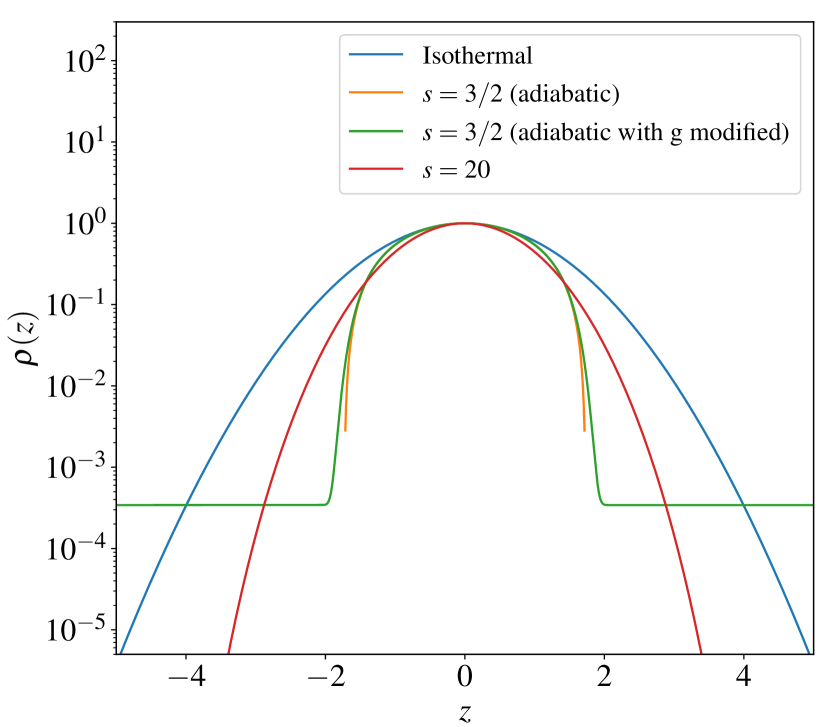
Figure 1: Density equilibrium profiles used in Section 3 and 4, serving as a background support for the spiral density waves. The green curve corresponds to an adiabatic profile with a modified gravity so that that the density converges toward a small constant value at large $z$. It is used in order to avoid a density floor in the adiabatic simulations of Section 4.

In Section 3 and 4, we neglect self-gravity and assume that waves propagate through a polytropic disc equilibrium, in which the pressure is given by

$$P=K\rho^{1+1/s},\quad\quad\text{with}\quad K=\dfrac{c_{s_{0}}^{2}}{\gamma\rho_{0}^{1/s}},$$ (8)

where the subscript “0" denotes the quantities in the midplane. We emphasize that this polytropic relation is adopted only as an initial equilibrium and does not account for the equation of state The case $\gamma=1$, $s=\infty$ corresponds to an isothermal atmosphere. An adiabatic atmosphere corresponds to $\gamma=1+1/s=5/3$ (i.e $s=3/2$), while for a general polytrope with stable stratification, we have $s<3/2$. The entropy gradient is zero in the adiabatic case, while in the polytropic case it is related to the Brunt-Väisälä frequency $N^{2}$ through

$$\dfrac{ds}{dz}=\dfrac{c_{V}\gamma N^{2}}{g(z)}=c_{V}(1+1/s-\gamma)\dfrac{d\log{\rho}}{dz}.$$ (9)

Taking a general vertical gravity ${g}(z)$ and applying the vertical hydrostatic balance, the density profile of the equilibrium can be integrated analytically:

$$\rho(z)=\rho_{0}\left(1-\dfrac{1/s}{(1+1/s)\Omega^{2}}\dfrac{\gamma}{H_{0}^{2}}\int^{z}_{0}\mid{g}(z)\mid dz\right)^{s}.$$ (10)

For almost all cases considered we use the thin disc approximation, for which the vertical gravity induced by the central object is

$$g(z)=-\Omega^{2}z.$$ (11)

Figure 1 shows some density profiles corresponding to the isothermal case, to $s=3/2$, and to $s=20$. Note that for an isothermal equation of state, Eq. (10) does not apply and the profile is the classical Gaussian $\propto\exp(-z^{2}/H_{0}^{2})$. For the other profiles, the density goes to 0 at a finite distance $H_{c}=\sqrt{2(s+1)/\gamma}\,H_{0}$ from the midplane.

2.4 Numerical methods

In Section 3, we linearise equations (1)-(3) and solve for the free axisymmetric modes by using an eigensolver based on a Chebyshev collocation method on a Gauss-Lobatto grid. This method results in a matrix eigenvalue problem that can be solved using the QZ algorithm (Golub & Van Loan, 1996; Boyd, 2001). Numerical convergence is guaranteed by comparing eigenvalues at different grid resolutions and eliminating the spurious ones. We apply a free surface boundary condition at the vertical domain boundaries $z=L_{z}/2$ and $-L_{z}/2$ with zero Lagrangian pressure, as in Korycansky & Pringle (1995, hereafter KP95). We tested our solver by comparing eigenvalues and eigenfunctions with those of KP95 and found very good agreement; in addition some of the calculations were repeated with a shooting method similar to that of KP95 .

In Section 4 and 5, direct simulations of equations (1)-(3) are performed using the Godunov-based PLUTO code (Mignone et al., 2007). The numerical scheme employs a conservative finite-volume method that solves the approximate Riemann problem at each inter-cell boundary. Our simulations are computed in a shearing box of size $(L_{x},L_{y},L_{z})$ and resolution $(N_{X},N_{Y},N_{Z})$. Note that because PLUTO conserves the total energy, the heat equation Eq.(3) is not solved directly. The code, consequently, captures the irreversible heat produced by shocks due to numerical diffusion, consistent with the Rankine Hugoniot conditions. Boundary conditions are periodic in $y$ and shear-periodic in $x$. In the vertical direction we use a standard outflow condition for the velocity field but compute a hydrostatic balance in the ghost cells for pressure. As the problem studied varies from Section 4 to Section 5, more details about box size, resolution, initialization, and others parameters are given in the corresponding sections.

3 Linear axisymmetric theory and roll structure

In order to set the scene, this section briefly revisits the linear theory of unforced axisymmetric waves in a polytropic disc without self-gravity and highlight their vertical structure. Though obviously not spiral waves, they nevertheless encapsulate most of the physics we are interested in, especially when in the tightly wound limit. Direct connections with simulated spiral density waves will be made in Section 4.

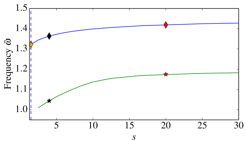
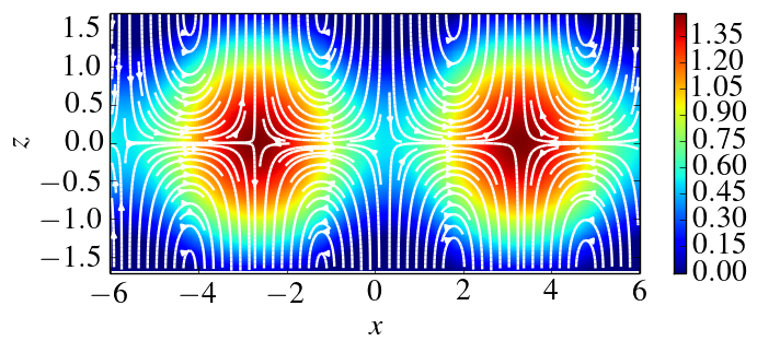
Figure 2: Top: Frequencies of the fundamental axisymmetric p-mode and g-mode $(n=0)$ as a function of the polytropic index $s$ and for $k_{x}=(\pi/3)H_{0}^{-1}$. Bottom: density and poloidal streamlines of the fundamental axisymmetric p-mode in an adiabatic atmosphere ($s=3/2$) for the same $k_{x}$. The density shown here is $\rho_{e}+0.6\hat{\rho}$

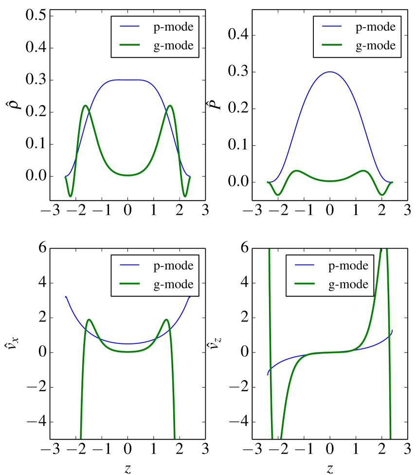
Figure 3: Eigenfunctions of the fundamental p-mode (blue) and g-mode (green) for $s=4$ and $k_{x}=(\pi/3)H_{0}^{-1}$. Top panels: perturbed density (left) and pressure (right). Bottom panels: perturbed radial (left) and vertical (right) velocities

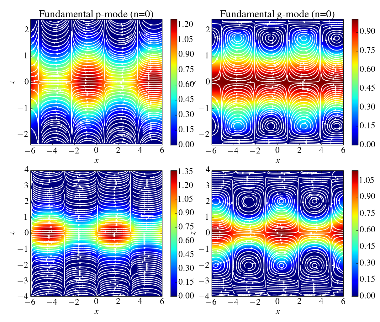
Figure 4: Density and poloidal streamlines of the fundamental axisymmetric p-mode (left) and g-mode (right) for $k_{x}=(\pi/3)H_{0}^{-1}$. Top panels are for $s=4$ while bottom panels are for $s=20$. The density shown here is $\rho_{e}+0.6\hat{\rho}$.

We denote by ${\rho}_{e}(z)$ and $P_{e}(z)$ the equilibrium profiles of density and pressure, defined in Section 2.3. We add density, velocity, and pressure perturbations of the form $\left[\hat{\rho}(z),\,\hat{\mathbf{u}}(z),\hat{{P}}(z)\right]\,\exp(\text{i}k_{x}x-\text{i}\omega t)$. The densities (background and perturbations) are then normalised by the midplane density $\rho_{0}$, velocities by the uniform sound speed $c_{s_{0}}$, and pressure by $\rho_{0}c_{s_{0}}^{2}$. Finally we introduce the dimensionless wave frequency $\bar{\omega}=\omega/\Omega$ and wavelength $\bar{k}_{x}=k_{x}H_{0}$ with $H_{0}=c_{s_{0}}/\Omega$. The linearised and normalized system of equations reads

$$-\text{i}\bar{\omega}\hat{\rho}+\text{i}\bar{k}_{x}\rho_{e}\hat{u}_{x}+\dfrac{d}{d\bar{z}}(\rho_{e}\hat{u}_{z})=0,$$ (12)

$$\rho_{e}(-\text{i}\bar{\omega}\hat{u}_{x}-2\hat{u}_{y})=-\text{i}\bar{k}_{x}\hat{P},$$ (13)

$$\rho_{e}(-\text{i}\bar{\omega}\hat{u}_{y}+\dfrac{1}{2}\hat{u}_{x})=0,$$ (14)

$$\rho_{e}(-\text{i}\bar{\omega}\hat{u}_{z})=-\dfrac{d\hat{P}}{d\bar{z}}-\hat{\rho}\bar{z},$$ (15)

$$-\text{i}\bar{\omega}\hat{P}+\text{i}\bar{k}_{x}P_{e}\hat{u}_{x}+\dfrac{d}{d\bar{z}}(P_{e}\hat{u}_{z})=-P_{e}(\gamma-1)(\dfrac{d\hat{u}_{z}}{d\bar{z}}+\text{i}\bar{k}_{x}\hat{u}_{x}).$$ (16)

Solutions to these equations have been obtained by KP95 and Ogilvie (1998). The system supports three solution families: one at “low" frequency with $\bar{\omega}<1$, which corresponds to inertial modes (r-modes), and two at “high" frequency with $\bar{\omega}>1$, which correspond to acoustic modes (p-modes) and buoyancy modes (g-modes). Each family is composed of a countable set of branches, where each branch is labelled by an integer $n$ characterising the mode vertical wavenumber. The two fundamental even $n=0$ and odd $n=1$ p-modes are often referred as f-modes or free surface oscillations, though they are also the 3D manifestation of 2D density waves and their properties are very different from the stellar f-modes (KP95, Mamatsashvili & Rice, 2010)

We focus on the $n=0$ fundamental p and g-modes for a wavenumber $k_{x}=\pi/3$; thus the waves are radially large-scale. The heat capacity ratio is set to $\gamma=5/3$. The numerical domain extends from $z=0$ to $z=L_{z}=H_{c}=\sqrt{2(s+1)/\gamma}$, the latter corresponding to the disc surface beyond which $\rho_{e}$ and $P_{e}$ are precisely 0. The eigenfunctions are resolved by 300 points in the $z$ direction.

Figure 2 (top) shows the angular frequencies of the fundamental $n=0$ p-mode (blue curve, upper branch) and g-mode (green curve, lower branch) as a function of the polytropic index $s$. We first analyse the p-mode in the adiabatic case $s=3/2$ (yellow diamonds on the top branch). Fig. 2 (bottom) shows the total density (background plus perturbations) and the poloidal streamlines associated with the eigenmode. The streamlines show non-circulating vertical motions, which can be interpreted as a free surface oscillation characteristic of the large-scale density wave. We should emphasise at this point that streamlines are not pathlines, and so the fluid displacements associated with the waves will be small on account of them being in the (low-amplitude) linear regime.

We next plot the shape of the fundamental p-mode and g-mode for $s=4$ (black markers in Fig. 2). Appearing in Fig. 3 are the normalized eigenfunctions for both modes and in Fig. 4 (top), the total density and poloidal streamlines of the corresponding mode. Clearly, the p-mode has the same shape as in the adiabatic case, while the g-mode exhibits roll structures located below the disc surface. Fig. 3 (bottom) shows that the same behaviour is obtained for larger $s=20$. We remind the reader that self gravity has been omitted in these calculations. We checked independently that these structures are also obtained when solving for the linear g-modes of a self-gravitating disc with Toomre $Q=1.6$.

In conclusion, low amplitude axisymmetric waves exhibit vertical circulation (rolls) in the sub-adiabatic regime. These are most pronounced in the profiles of the (stable) g-modes, whereas the modes associated with low-amplitude density waves do not exhibit such vortical structures.

4 Vertical structure of spiral waves forced by a potential

In this section, we treat forced, non-axisymmetric, and highly nonlinear waves, such as those excited by tidal interactions or GI. For that purpose, we simulate in the shearing box the behaviour of individual 3D spiral waves excited by an external potential.

4.1 Simulation setup and wave excitation

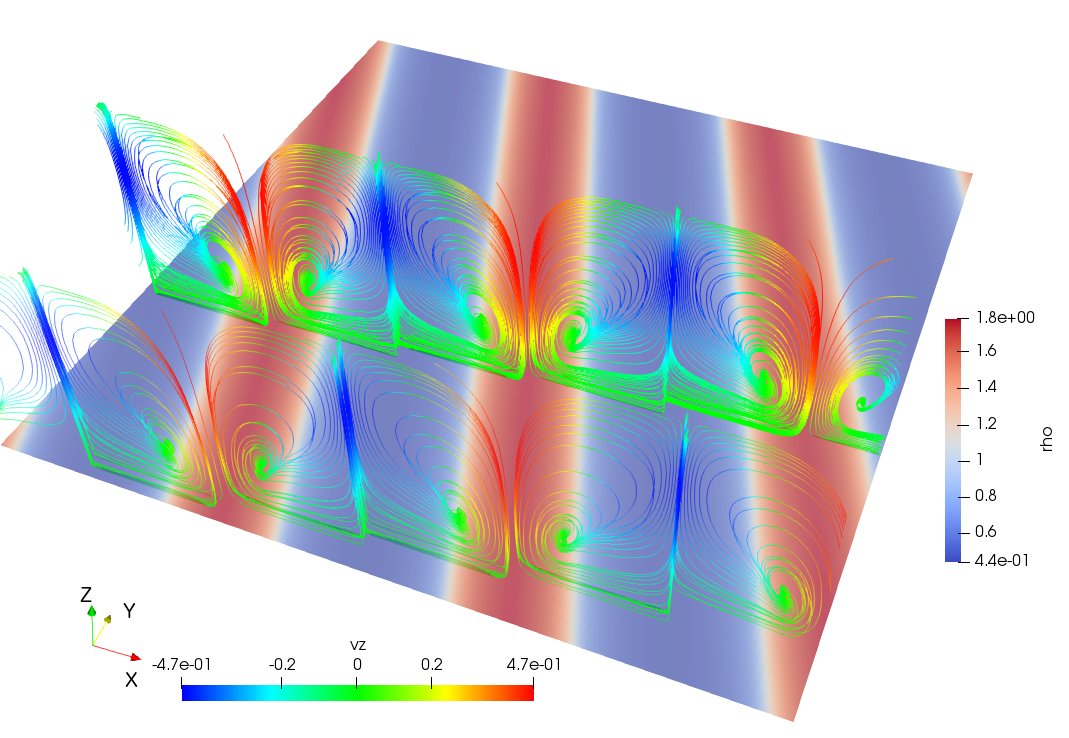
Figure 5: Top: 3D view of a spiral wave structure simulated with PLUTO in a polytropic disc atmosphere with $s=20$, and forcing amplitude $A=0.25$ (nonlinear regime). The wave density is represented in the midplane while the coloured lines are the streamlines projected in the poloidal plane. The colour of the streamlines denote the vertical velocity.

In order to characterize the fundamental motions associated with these waves, we restrict ourselves to a simple configuration, omitting self-gravity and retaining very basic thermodynamics (no cooling law). Our box spans $10H_{0}$ in the radial and azimuthal directions, and $\pm 3H_{0}$ in the vertical direction. We start the simulations with different hydrostatic equilibria: isothermal, adiabatic, and polytropic (described in Section 2.3). Note that in the case of an adiabatic profile, $H_{c}\approx 1.73H_{0}$ is small compared to the vertical extent of the simulation domain $z=\pm 3H_{0}$, meaning that in most of the box the density is strictly zero, a numerical difficulty. One way to circumvent this problem is to impose a density floor beyond the altitudes $\pm H_{c}$. But doing so generates a strong shock associated with downfalling material. This shock produces a spurious entropy gradient capable of artificially producing vertical rolls. A better alternative to the density floor is to use a slightly modified gravitational acceleration (in the adiabatic case only), such as

$$g(z)=-\Omega^{2}z\exp(-z^{16}/r_{0}^{16}),$$ (17)

with $r_{0}=1.78\,H_{0}$. The resulting density profile, shown in Fig. 1 is indiscernible from the original (thin disk) profile for $z<1.73\,H_{0}$ and tends toward a fixed value of $\sim 3\times 10^{-4}$ at higher altitude. No spurious entropy is generated and yet the sharp density drop is well approximated at $z\simeq 1.73\,H_{0}$.

Once the equilibrium is given, the spiral waves are excited by an external potential of the form:

$$\Phi_{\text{ext}}=A\,\cos\left[k_{x}(t)x+mk_{y_{0}}y\right],$$ (18)

where $A$ is the amplitude of the forcing and $k_{x}(t)=-k_{x_{0}}+Sk_{y_{0}}t$, with $k_{x_{0}}=2\pi/L_{x}$ and $k_{y_{0}}=2\pi/L_{y}$ the fundamental wavenumbers of the numerical domain. We voluntarily impose no vertical dependence on the potential, so that no vertical motions are directly forced. To a first approximation, this potential reproduces the stirring of the gas by a 2D self-gravitating potential as witnessed in simulations of gravitoturbulence. Therefore, if vertical motions appear, they result logically from the intrinsic spiral wave dynamics.

The non-axisymmetric waves excited are not periodic solutions of the fluid equations, but are rather dynamical. They are first amplified by the potential during their leading phase ($k_{x}(t)k_{y}<0$, between $t=0$ and $t=S^{-1}L_{y}/L_{x}=2/3\,\Omega^{-1}$) and then becomes trailing. After a few $\Omega^{-1}$, they reach a maximum and then decay because of the shear and numerical dissipation. An example spiral wave is shown in Fig. 5 at $t=2.5\Omega^{-1}$ (during the late trailing phase), for a disc polytropic index $s=20$ and a forcing amplitude $A=0.25$.

Figure 6: Poloidal structure of spiral density waves in the isothermal (top), adiabatic ($s=3/2$, middle) and sub-adiabatic atmosphere ($s=20$, bottom). The amplitude of the forcing in the left panels is $A=0.05$ (linear forcing). In the right panels, this amplitude is larger, $A=0.4$, $A=1$, $A=0.25$ from top to bottom respectively (nonlinear forcing). The colourmap indicates the density while the cyan curves are the streamlines in the poloidal plane. Snapshots are taken at $t\simeq 2.5\,\Omega^{-1}$.

Figure 7: Top: density and poloidal streamlines for $A=1$ in an adiabatic atmosphere ($s=3/2$). Bottom: vorticity in the $y$ direction; the arrows represent the direction of the temperature (white) and entropy (black) gradients. Right and left panels are at $t=2.4\Omega^{-1}$ and $t=2.7\Omega^{-1}$ respectively.

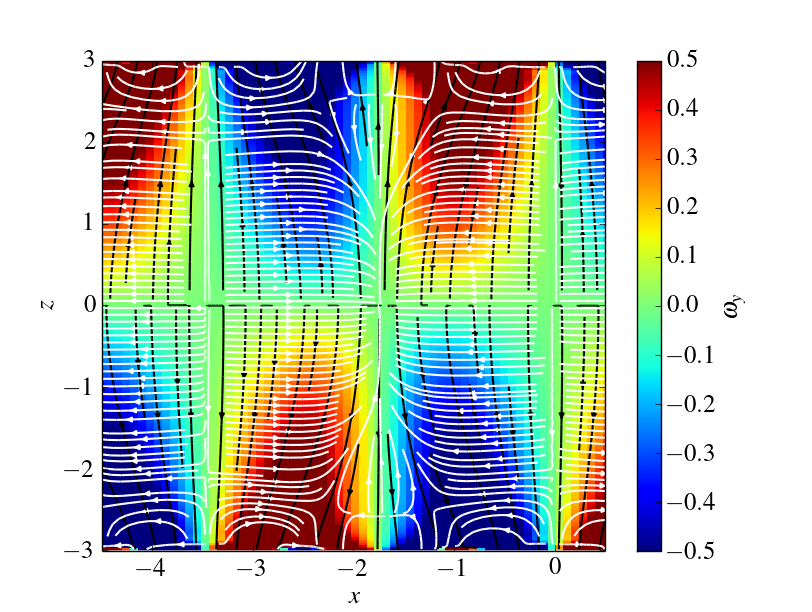
Figure 8: Vorticity in the $y$ direction for the case $s=20$ and $A=0.05$ (top) and $A=0.3$ (bottom); the snapshot is zoomed in on one spiral arm of Fig. 6. The arrows represent the direction of the temperature (white) and entropy (black) gradients.

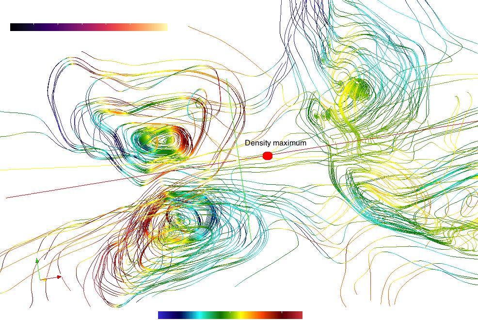
Figure 9: Streamlines associated with a spiral wave in a shearing box simulation of GI. The top panel is a view from the top (looking down to the midplane) while the bottom panel is a poloidal cut (view from the disc midplane) with the angular momentum vector pointing upward. The red line in the bottom panel indicates the midplane $z=0$. The colour of the streamlines represent in both cases the amplitude of the velocity component $v_{z}$

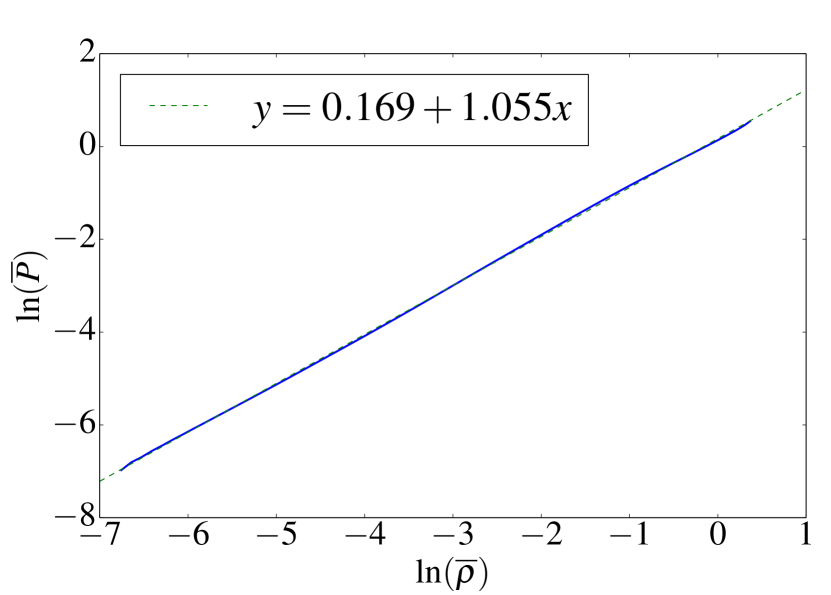
Figure 10: Disc stratification in the gravito-turbulent simulation of Riols et al. (2017). The plain blue curve represents the mean pressure profile in $z$ as a function of the mean density profile in $z$, calculated from the turbulent data (in log space). The dashed green curve is a linear fit of the plain curve. Clearly, $\overline{P}\propto\overline{\rho}^{1.05}$.

4.2 Linear regime

We first perform simulations of 3D spiral waves in the linear regime, with a weak forcing $A=0.05$ and a resolution $N_{X}=N_{Y}=128$ and $N_{Z}=256$.

4.2.1 Isothermal

When using an isothermal equation of state and an initial Gaussian hydrostatic profile, the forced spiral waves exhibit a relatively simple vertical structure. Their poloidal motion consists of simple compression/expansion and the streamlines remain purely horizontal, as shown in the top left corner of Fig. 6. (Higher order p-mode harmonics (larger $n$) display non-negligible vertical displacements but these do not emerge naturally from a pure horizontal forcing, nor could be classified as ‘density waves’.) If we leave aside the non-axisymmetry, the mode forced here is similar to the free two-dimensional acoustic–inertial mode $n=0$, which is the first mode that becomes unstable to GI in isothermal disc (see Appendix B in Riols et al., 2017).

4.2.2 Adiabatic

In contrast to the isothermal case, waves in an adiabatic stratification (with $s=3/2$) rapidly develop vertical motions. Between $t=0$ and $t=2\,\Omega^{-1}$, the gas undergoes vertical ascending motion at the radius where the density is maximum and a descending motion where it is minimum (see centre-left panel of Figure 6). The flow configuration resembles that of the unforced axisymmetric wave (see bottom panel of Fig. 2 for a comparison). In the highly compressed region $\nabla\cdot\mathbf{\delta u}<0$ and the pressure work is positive. It induces a $\delta P>0$ with positive vertical gradient $\nabla\delta P>0$, making the flow rise up. On the other hand, in the expanding region, $\nabla\cdot\mathbf{\delta u}>0$ and the pressure fluctuation is negative but smaller in the corona. In this case, the pressure difference drives the flow toward the midplane. It must be said, however, that it is inappropriate to designate the motion as “circulating" because the flow does not form closed loops and turns parallel at large $z$.

Ultimately, after $t=2\Omega^{-1}$ (not shown here), the topology of the flow alters and the streamlines change their orientation because the gas expands in the densest regions. In the bulk of the disc ($z<H_{0}$), the vertical motions become oriented toward the midplane. All streamlines converge to the same point which corresponds to the density minimum. We checked that no vortical structure appears during the late trailing phase of the linear wave.

4.2.3 Sub-Adiabatic

Fig. 6 (bottom left) shows the poloidal streamlines for $s=20$ which corresponds to a sub-adiabatic stratification. This profile mimics a disc in which the corona is heated by an external source or by turbulent motions rather than pressure work. As we will show later in Section 5, it adequately describes simulations of GI turbulent discs, which usually show flat temperature profiles.

In this regime, we found that in the linear regime, spiral waves exhibit large-scale poloidal rolls, orbiting or spiralling toward a central point. Each density maximum is surrounded by four counter-rotating cells, symmetric about the midplane. These coherent motions are maintained for $\sim 1\,\Omega^{-1}$. By scanning other polytropic indices, we found that proper rolls (with closed streamlines) also emerge for smaller $s$.

The vortical structures are similar to those exhibited by the unforced linear axisymmetric g-modes ($m=0$, see Fig. 4 for comparison). Note however that the density maxima in the simulated forced waves are located at the intersections of the rolls, but not in the unforced (free) linear axisymmetric calculation. Our explanation is that the gravitational forcing excites both the fundamental p-mode (density waves) and the fundamental g-mode. The density patterns are mainly due to the p-mode while the velocity components above the midplane are the expression of the g-mode. These two superimposed modes possibly interact weakly each other via nonlinear terms, providing the observed shape. The phase lag may result from this weak coupling. The physical origin of the rolls is discussed in Section 4.4.

4.3 Nonlinear regime

We now explore strongly nonlinear waves, for which the amplitude $A$ is adjusted in order to obtain a local Mach number $u/c_{s}$ larger than 1. We keep the same resolution as in the previous section.

In the pure isothermal case, increasing the amplitude of the forcing potential does not help the formation of vertical structures. For an amplitude $A\simeq 0.4$, Fig. 6 (top right) shows that the streamlines, projected in the poloidal plane, remains horizontal.

In the adiabatic atmosphere we examine two forcing amplitudes: $A=0.4$ and $A=1$. Figure 6 (centre-right panel) reveals that for a large amplitude $A=1$, the vertical wave structure at $t=2.5\Omega^{-1}$ is more complex than in the linear regime. A pair of rolls is produced and take the form of butterfly wings. However, the latter remain relatively short-lived and are less developed than in the linear sub-adiabatic regime. Fig. 7 (top panels) shows the streamlines before and after $t=2.5\Omega^{-1}$. As the flow rises up during the early trailing phase (left panel), a shock forms and deflects the streamline, producing vorticity (see next section). Later (right panel), the shock has been advected by the vertical circulation and almost disappears. At a smaller forcing amplitude $A=0.4$, corresponding approximatively to the transonic regime, the same behaviour is observed, but only marginally and the vortical motions generated are much less pronounced.

Finally, in the case of a subadiabatic polytrope with $s=20$ and a forcing of $A=0.3$, the spiral wave is characterised by well-developed vertical cells as shown in Figure 6 (bottom right). They are much stronger than in the nonlinear adiabatic case and expand further away into the corona. A weak shock is present and tends to bend the streamlines, preventing the rolls from being circular. It is important to note that, unlike the linear regime, the rolls extend all the way to the midplane and are probably much more efficient at mixing disc material throughout the vertical column. The 3D view in Fig. 5 shows that the poloidal wave pattern in the nonlinear regime maintains a translational symmetry along the density wake.

4.4 Physical origin of the rolls

In the adiabatic case, rolls appear only if the local Mach number of the wave exceeds unity. Figure 7 shows the poloidal streamlines (top panels) at two successive times, $t=2.4$ and $t=2.7\,\Omega^{-1}$, when the forcing is $A=1$. In the left panel, a shock is clearly visible and separates the expanding region (where the flow rises up) and the compressed region (where the flow converges toward the density maximum). Observe that the shock is not fixed but advected by the ascending flow. Therefore, the postshock region (or downstream velocity) is located above, where the gas expands. The bottom panels of Fig. 7 shows the vorticity and orientation of the entropy (black lines) and temperature (white lines) gradients. Vorticity is produced across the entropy jump at the shock interface. The misalignment between entropy and temperature gradients in the post-shock region contributes also to the vorticity production in this region via the baroclinic term $\mathbf{\nabla}S\times\mathbf{\nabla}T$ (see Eq. 7). The other terms in Eq. 7 are subdominant during this phase. In summary, rolls motions are driven by a nonlinear baroclinic effect, mediated by the entropy production across the shock wave.

In the sub-adiabatic case, the mechanism differs, since rolls emerge even in the linear theory; we argued in Section 4.2.3 that they are the signatures of large-scale g-modes excited alongside the density wave. But what is the physical mechanism driving these rolls? Fig. 8 (top) shows that for a small forcing amplitude $A=0.05$, vorticity is concentrated along butterfly “wings" where entropy and temperature gradient are orthogonal. The poloidal rolls are then clearly produced through the baroclinic term. Unlike the adiabatic case, a vertical entropy gradient is already present, inherited from the background stratification. No shocks are required. The temperature gradient has a strong radial component, resulting from the pressure work due to wave compression. Fig. 8 (bottom) shows that the same patterns are seen in the nonlinear regime, although the temperature gradients are less horizontal, in particular near the shock region. Additional vorticity is provided by the entropy jump across the discontinuity and tends to deflect the streamlines, in a manner similar to the adiabatic case.

5 Spiral waves in gravito-turbulent discs

In this section, we study the vertical dynamics of spiral density waves excited by GI. Our goal is to check if the vertical motions described in the previous section are robust and can be obtained in a turbulent background with cooling typical of young PP discs.

5.1 Initial condition and simulation setup

To begin, we performed a turbulent disc simulation with GI. The simulation is initialized from a 3D gravito-turbulent state obtained from Riols et al. (2017) (the run is labelled PL20-512 in the corresponding paper). The numerical methods and simulation setup are detailed in the related paper. We remind the reader that self-gravity is computed by solving the Poisson equation numerically (Eq. 5). To solve this equation, we perform a decomposition of the density and potential in 2D Fourier space ($k_{x}$,$k_{y}$) for each slice in $z$. The boundary conditions in the vertical direction are non-periodic and given in Riols et al. (2017). The vertical domain extends from $-3H_{0}$ to $3H_{0}$ and the horizontal box size is $L_{x}=L_{y}=20\,H_{0}$. The resolution is $512\times 512\times 64$, so that one scale-height is resolved by $\sim 26$ points. To make a steady gravito-turbulent state possible, we introduced a cooling law $\Lambda^{-}=P/\tau_{c}$ in the internal energy equation (3) where $\tau_{c}=20\,\Omega^{-1}$ is a typical timescale referred to as the ‘cooling time’. This prescription is not necessarily realistic but allows us to control the rate of energy loss via a single parameter.

5.2 Spiral waves and vertical rolls

The gravito-turbulent simulation describes a flow composed of large-scale spiral density waves, small-scale incompressible waves, and clumpy structures. We focus here on the dynamics around one spiral wave chosen randomly within the turbulent flow. Fig 9 shows the 3D topology of the streamlines around this spiral wave. The density wake can be seen in the coloured rendering of the density $\rho$ in the top panel, which appears bright and pale when high, and dark in more evacuated regions. Superimposed upon the wake are the flow streamlines coloured according to the magnitude (and sign) of $v_{z}$. The bottom panel is a poloidal cut of the same wake, with the red straight line indicating the midplane and the green straight line the vertical axis. The green axis cuts through the centre of the density wake in the upper panel.

In the bottom panel, we can clearly distinguish on the left of the density wake two (somewhat tangled) large rolls, with streamlines forming closed loops. The sign of $v_{z}$ indicates the the upper roll rotates counter-clockwise, while the lower roll rotates clockwise. Both are of scale $H$ and symmetric (on average) about the midplane. On the right of the density wake, the flow is much more disorganised but again one can discern two roll-like structures; they are fainter and rotating in the opposite direction. Overall, the streamlines form a pattern similar to those depicted in Fig. 5 and Fig. 6 (bottom). They are however more disorganised, somewhat understandably, as they emerge from a turbulent background.

To make a comparison with our simple atmosphere model of Section 4, we estimate the typical index $s$ measuring the disc stratification in our GI simulations. Figure 10 shows the mean vertical pressure profile $\overline{P}$ as a function of the mean density profile $\overline{\rho}$, in logarithm scale. Each profile is averaged over time, $x$ and $y$. The result shows a clear linear trend, suggesting that the polytropic model is an excellent fit to the mean gravito-turbulent vertical structure. The slope of the curve gives $1+1/s\simeq 1.05$, i.e $s\simeq 20$, which is the polytropic index used in Section 4. Therefore, there is clear indication that the vertical rolls are driven by the vertical entropy gradient naturally generated by the turbulent motions in these discs. However, we emphasize that this gradient might be sensitive to the cooling law and numerical details of the simulations. It is probably an under-estimate, given that a real disc is usually irradiated by FUV radiation, X-rays, and cosmic rays, physics that is not taken into account in our simulations.

Finally, we checked that these structures appear in other spiral arms and occur frequently in the simulation. We point out that the roll structures do not survive more than a few $\Omega^{-1}$, and die once their parent density waves break down. The rolls motions are transonic and represent a large fraction of the r.m.s velocity. They account for most of the vertical kinetic energy in the disc corona and are clearly responsible for the increase of both the r.m.s radial and vertical velocity with altitude (see Fig . 2 of Riols et al. (2017)). Note that in addition to the large scale rolls, a small-scale vertical component arising from a parametric instability has been also identified in this simulation (see Riols et al., 2017).

6 Discussion and conclusions

In summary, we have shown using shearing-box simulations that large-scale spiral waves in astrophysical discs exhibit vertical and vortical gas motions of size comparable to the disc height-scale. For an adiabatic atmosphere $1+1/s=\gamma=5/3$, these structures appear if the wave achieves shock amplitudes, but they are rather difficult to produce and have a short lifetime. When the polytropic index is lower ($1+1/s<\gamma$), vortical structures are much easier to trigger: they appear even in the subsonic regime and live longer. In this case, the flow is characterised by four counter-rotating cells, symmetric about the midplane, potentially transporting material from overdense regions towards the surface. These structures are enhanced in the nonlinear regime and penetrate to the midplane. Finally, we found that roll motions are ubiquitous in gravito-turbulent disc simulations and are clearly related to the spiral wave dynamics induced by the gravitational instability. They appear to resist the small-scale turbulent background characterising these types of flows (see Riols et al. (2017)).

We investigated the origin of these motions and found that they issue from the baroclinicity possible in the system. The effect is enhanced if the disc is sub-adiabatic (stably stratified) with a large scale (stable) entropy gradient. In contrast, rolls in adiabatic disks requires sufficiently large wave amplitudes and associated shocks. Our semi-analytic and linear axisymmetric calculations reveal that the rolls are associated with the fundamental (buoyancy) g-mode, which appears to emerge alongside the density wave. The alternative mechanisms mentioned in the introduction (vertical breathing/splashing, convection) might be also relevant for the spiral wave dynamics but are not essential in the production of rolls of typical size $\gtrsim H$.

Our results have several implications for young protoplanetary disks especially. Poloidal rolls may convey small grains (with stopping times much less than $\Omega^{-1}$) as far as the corona if the associated density waves are of sufficient amplitude and live sufficiently long. Obviously, this physics could bear directly on dust concentration and sedimentation processes in those PP discs subject to GI or disturbances originating from embedded planets and binary companions. In particular, vertical circulation may interfere with dust agglomeration in gravitoturbulence. Current simulations of GI-induced filamentary structure are 2D (Gibbons et al., 2012, 2014, 2015; Shi et al., 2016) and cannot describe the 3D vertical circulation revealed here. Quite separately, dust can also be mixed in the upper atmosphere by a parametric instability attacking the spiral waves themselves (Bae et al., 2016; Riols et al., 2017), and this could also affect the agglomeration process.

The roll motions could have an indirect impact on the scattered infra-red luminosity measured from observations. If the vertical lofting is efficient, dust may settle above the spiral patterns at the disc surface, altering its emission properties. In discs with an embedded planet this could bear on the estimation of the density contrast of the spiral arm and the subsequent inference of the planet’s mass (see Juhász et al., 2015, for more details on the original problem). We, however, emphasize that there are two main caveats to this effect. First there is generally a relative azimuthal velocity between dust particles and the spiral wave front. In that case, the lift will be significant if the time dust spends within the spiral structure is comparable to the rolls’ turnover time. This is probably true in the co-rotation region of the spiral wave (near the planet) but less obvious further away where the relative azimuthal velocity between dust particles and the wave front is significant. In gravitoturbulence, this issue is probably less important since spiral waves are almost co-rotating with the disc and are excited almost uniformly in the unstable region. Second, we stress that streamlines are different than pathlines, since the spiral waves propagate radially. For instance, in the linear regime, the motion of a test particle does not follow the vertical rolls and by definition, has only a small displacement. Thus, the wave needs to be sufficiently strong for the dust to rise. To quantify these different effects and make more accurate predictions, simulations of the dust-gas interaction in the vicinity of spiral waves or in 3D gravitoturbulence need to be performed and will be the object of a future paper.

A final application of this result is to the question of large-scale magnetic field generation in astrophysical discs generally. Recent simulations by Riols & Latter (2017) revealed that the spiral wave dynamics induced by GI can act as a powerful dynamo. The four counter-rotating roll motions identified in this study (combined with the shear) provides large-scale helicity and hence may efficiently amplify a seed magnetic field. In fact, the velocity structures are similar to the Ponomarenko or Roberts flows, which are known to provide kinematic dynamo action. One could then imagine a large-scale dynamo based on the successive action of spiral waves, although further work is required to understand if such a dynamo could work in gravito-turbulent discs, especially in the presence of the non-ideal MHD regimes relevant for PP disks.

References

- Bae et al. (2016) Bae J., Nelson R. P., Hartmann L., 2016, ApJ, 833, 126
- Benisty et al. (2015) Benisty M., et al., 2015, AAp, 578, L6
- Boley & Durisen (2006) Boley A. C., Durisen R. H., 2006, ApJ, 641, 534
- Boley et al. (2006) Boley A. C., Mejía A. C., Durisen R. H., Cai K., Pickett M. K., D’Alessio P., 2006, ApJ, 651, 517
- Boyd (2001) Boyd J. P., 2001, Courier Dover
- Chiang & Youdin (2010) Chiang E., Youdin A. N., 2010, Annual Review of Earth and Planetary Sciences, 38, 493
- Christiaens et al. (2014) Christiaens V., Casassus S., Perez S., van der Plas G., Ménard F., 2014, ApJl, 785, L12
- Dong et al. (2015) Dong R., Zhu Z., Rafikov R. R., Stone J. M., 2015, ApJl, 809, L5
- Durisen et al. (2007) Durisen R. H., Boss A. P., Mayer L., Nelson A. F., Quinn T., Rice W. K. M., 2007, Protostars and Planets V, pp 607–622
- Gammie (2001) Gammie C. F., 2001, ApJ, 553, 174
- Gibbons et al. (2012) Gibbons P. G., Rice W. K. M., Mamatsashvili G. R., 2012, MNRAS, 426, 1444
- Gibbons et al. (2014) Gibbons P. G., Mamatsashvili G. R., Rice W. K. M., 2014, MNRAS, 442, 361
- Gibbons et al. (2015) Gibbons P. G., Mamatsashvili G. R., Rice W. K. M., 2015, MNRAS, 453, 4232
- Goldreich & Tremaine (1979) Goldreich P., Tremaine S., 1979, ApJ, 233, 857
- Golub & Van Loan (1996) Golub G., Van Loan C., 1996, Matrix Computations. Johns Hopkins Studies in the Mathematical Sciences, Johns Hopkins University Press, https://books.google.fr/books?id=mlOa7wPX6OYC
- Grady et al. (2013) Grady C. A., et al., 2013, ApJ, 762, 48
- Juhász et al. (2015) Juhász A., Benisty M., Pohl A., Dullemond C. P., Dominik C., Paardekooper S.-J., 2015, MNRAS, 451, 1147
- Korycansky & Pringle (1995) Korycansky D. G., Pringle J. E., 1995, MNRAS, 272, 618
- Lesur et al. (2015) Lesur G., Hennebelle P., Fromang S., 2015, AAp, 582, L9
- Lin & Papaloizou (1979) Lin D. N. C., Papaloizou J., 1979, MNRAS, 186, 799
- Loska (1986) Loska Z., 1986, ACTAA, 36, 43
- Lubow & Ogilvie (1998) Lubow S. H., Ogilvie G. I., 1998, ApJ, 504, 983
- Lubow & Pringle (1993) Lubow S. H., Pringle J. E., 1993, ApJ, 409, 360
- Lyra et al. (2016) Lyra W., Richert A. J. W., Boley A., Turner N., Mac Low M.-M., Okuzumi S., Flock M., 2016, ApJ, 817, 102
- Mamatsashvili & Rice (2010) Mamatsashvili G. R., Rice W. K. M., 2010, MNRASs, 406, 2050
- Mann et al. (2015) Mann R. K., Andrews S. M., Eisner J. A., Williams J. P., Meyer M. R., Di Francesco J., Carpenter J. M., Johnstone D., 2015, ApJ, 802, 77
- Mignone et al. (2007) Mignone A., Bodo G., Massaglia S., Matsakos T., Tesileanu O., Zanni C., Ferrari A., 2007, ApJs, 170, 228
- Ogilvie (1998) Ogilvie G. I., 1998, MNRAS, 297, 291
- Pérez et al. (2016) Pérez L. M., et al., 2016, Science, 353, 1519
- Perrin et al. (2009) Perrin M. D., Schneider G., Hines D. C., Wisniewski J. P., Grady C. A., HST GO-11155 Team 2009, in American Astronomical Society Meeting Abstracts #213. p. 208
- Riols & Latter (2017) Riols A., Latter H., 2017, preprint, (arXiv:1709.06845)
- Riols et al. (2017) Riols A., Latter H., Paarekooper S.-J., 2017, MNRAS, pp 2223–2237
- Shi et al. (2010) Shi J., Krolik J. H., Hirose S., 2010, ApJ, 708, 1716
- Shi et al. (2016) Shi J.-M., Zhu Z., Stone J. M., Chiang E., 2016, MNRAS, 459, 982
- Stolker et al. (2016) Stolker T., et al., 2016, AAp, 595, A113
- Tobin et al. (2013) Tobin J. J., et al., 2013, ApJ, 779, 93
- Toomre (1964) Toomre A., 1964, ApJ, 139, 1217
- Ward (1986) Ward W. R., 1986, Icarus, 67, 164
- Zhu et al. (2015) Zhu Z., Dong R., Stone J. M., Rafikov R. R., 2015, ApJ, 813, 88