Finding Influential Training Samples for Gradient Boosted Decision Trees

Abstract

We address the problem of finding influential training samples for a particular case of tree ensemble-based models, e.g., Random Forest (RF) or Gradient Boosted Decision Trees (GBDT). A natural way of formalizing this problem is studying how the model’s predictions change upon leave-one-out retraining, leaving out each individual training sample. Recent work has shown that, for parametric models, this analysis can be conducted in a computationally efficient way. We propose several ways of extending this framework to non-parametric GBDT ensembles under the assumption that tree structures remain fixed. Furthermore, we introduce a general scheme of obtaining further approximations to our method that balance the trade-off between performance and computational complexity. We evaluate our approaches on various experimental setups and use-case scenarios and demonstrate both the quality of our approach to finding influential training samples in comparison to the baselines and its computational efficiency.

1 Introduction and Background

As machine learning-based models become more widespread and grow in both scale and complexity, methods of interpreting their predictions are increasingly attracting attention from the machine learning community. Some of the applications and benefits of employing these methods outlined in previous work (Ancona et al., 2017) include (1) “debugging” the model to expose ways of model failures not discoverable via conventional test set performance measuring (e.g., data or target leakages); (2) boosting developer’s trust in the model’s performance in scenarios when on-line evaluation is not available before deployment; and (3) increasing user satisfaction and/or confidence in provided predictions, etc . Various problem setups (Palczewska et al., 2013; Tolomei et al., 2017; Fong & Vedaldi, 2017) and interpretation methods, both model-agnostic (Ribeiro et al., 2016; Lundberg & Lee, 2017) and model-specific (Shrikumar et al., 2017; Tolomei et al., 2017; Sundararajan et al., 2017), have recently been proposed in the literature.

A common trait shared by the majority of these methods is that they treat the provided model as a fixed function of input objects and study which features had the largest effect on the prediction, how the model responds to feature perturbations, etc. However useful they are, the obtained interpretations do not provide a way of automatically improving the model, since the model is fixed; the main use-case thus becomes manual analytics by the user or the developer, which is both time and resource-consuming. It is thus desirable to derive a framework for obtaining actionable insights into the model’s behavior allowing us to automatically improve a model’s performance.

One such framework has recently been introduced by Koh & Liang (2017); it deals with finding the most influential training objects. They formalize the notion of “influence” via an infinitesimal approximation to leave-one-out retraining: the core question that this work aims to answer is “how would the model’s performance on a test object $\mathbf{x}_{test}$ change if the weight of a training object $\mathbf{x}_{train}$ is perturbed?” Assuming a smooth parametric model family (e.g., linear models or neural networks), the authors employ the Influence Functions framework from classical statistics (Cook & Weisberg, 1980) to show that this quantity can be estimated much faster than via straightforward model retraining, which makes their method tractable in a real-world scenario. A natural use-case of such a framework is to consider individual test objects (or groups of them) on which the model performs poorly and either remove the most “harmful” training objects or prioritize a batch of new objects for labeling based on which ones are expected to be the most “helpful,” akin to active learning.

Unfortunately, the method suggested by Koh & Liang (2017) heavily relies on the smooth parametric nature of the model family. While this is a large class of machine learning models, it is by far not the only one. In particular, decision tree ensembles such as Random Forests (Ho, 1995, RF) and Gradient Boosted Decision Trees (Friedman, 2001, GBDT) are probably the most widely used model family in industry, largely due to their state-of-the-art performance on structured and/or multimodal data. Thus, it is important to extend the aforementioned Influence Functions framework to tree ensembles.

In this paper, we propose a way of doing so, while focusing specifically on GBDT. We consider two proxy metrics for the informal notion of influence. For the first one, leave-one-out retraining, we utilize the inner mechanics of fitting decision trees (in particular, assuming that a small training sample perturbation does not change the trees’ structures) to derive LeafRefit and FastLeafRefit, a well-founded family of approximations to leave-one-out retraining that trade off approximation accuracy for computational complexity. For the second, analogously to the Influence Functions framework, we consider infinitesimal training sample weight perturbations and derive LeafInfluence and FastLeafInfluence, methods for estimating gradients of the model’s predictions with respect to training objects’ weights. From a theoretical perspective, LeafInfluence and FastLeafInfluence allow us to deal with the discontinuous dependency of tree structure on training sample perturbations; from a practical one, they allow us to further reduce computational complexity due to the possibility of precomputing certain derivatives.

In our experiments we (1) study the conditions under which our methods, FastLeafRefit and FastLeafInfluence, successfully approximate their proxy metrics, (2) demonstrate our methods’ ability to target training objects which are influential for specific test objects, and (3) show that our algorithms run much faster than straightforward retraining, which makes them applicable in practical scenarios.

Table 1: Mathematical notations used in the paper.

Notation	Description
$\mathbf{x}=(x,y)$	Data point
$\mathbf{X}=\{(x_{i},y_{i})\}_{i=1}^{n}$	Training/test sample
$L(y_{true},y_{pred})$	Loss function
$\mathbf{w}=(w_{1},...,w_{n})$	Weights of training samples
$P(x)=(i_{1},...,i_{T})$	Path (leaf indices) of $x$
$F(x)$	GBDT prediction at point $x$
$f_{l}^{t}$	Value in leaf $l$ at step $t$
$I_{l}^{t}$	Training points belonging to leaf $l$ at step $t$
$\mathbf{A^{t}}=\{A_{i}^{t}:=\sum_{\tau=1}^{t}f_{P(x_{i})_{\tau}}^{\tau}\}_{i=1}^{n}$	Intermediate predictions on $\{x_{i}\}_{i=1}^{n}$
$g^{t}_{i}(A_{i}^{t-1}):=\frac{\partial L(y_{i},z)}{\partial z}|_{z=A_{i}^{t-1}}$	$i$-th first derivative at training step $t$
$h^{t}_{i}(A_{i}^{t-1}):=\frac{\partial^{2}L(y_{i},z)}{\partial z^{2}}|_{z=A_{i}^{t-1}}$	$i$-th second derivative at training step $t$
$k^{t}_{i}(A^{t-1}_{i}):=\frac{\partial^{3}L(y_{i},z)}{\partial z^{3}}|_{z=A_{i}^{t-1}}$	$i$-th third derivative at training step $t$
$G^{t}_{l}(\mathbf{A^{t-1}}):=\sum_{j\in I_{l}^{t}}w_{j}g^{t}_{j}(A_{j}^{t-1})$	Sum of leaf derivatives
$H^{t}_{H;l}(\mathbf{A^{t-1}}):=\sum_{j\in I_{l}^{t}}w_{j}h^{t}_{j}(A_{j}^{t-1})$	Sum of leaf second derivatives
$H^{t}_{G;l}(\mathbf{A^{t-1}}):=\sum_{j\in I_{l}^{t}}w_{j}$	Sum of leaf weights
$\mathit{Inf_{grad}}(\mathbf{x}_{1},\mathbf{x}_{2})$	Influence of object $\mathbf{x}_{1}$ on $\mathbf{x}_{2}$

2 Problem Definition

First, we formally define the problem setup. We consider standard supervised training of a GBDT ensemble $F(x;\mathbf{w}):=\sum_{t=1}^{T}f_{P(x)_{t}}^{t}(\mathbf{A^{t-1}})$ on a training sample $\mathbf{X}_{train}$. Learning consists of two separate stages: model structure selection and picking the optimal leaf values. The way of choosing the model structure is not important for our work; we refer the interested reader to existing implementations, e.g., Chen & Guestrin (2016); Dorogush et al. (2017). For picking optimal leaf values, we consider two most commonly used formulas:

Gradient: At leaf $l$ at step $t$, output negative average gradients (calculated at current predictions) over the leaf objects:

$$\begin{gathered}f_{G;l}^{t}(\mathbf{A^{t-1}}):=-\frac{G^{t}_{l}(\mathbf{A^{t-1}})}{H^{t}_{G;l}(\mathbf{A^{t-1}})}.\end{gathered}$$ (1)

This is equivalent to minimizing the empirical loss function w.r.t. the current leaf value by doing a single gradient step in function space (Chen & Guestrin, 2016).

Newton: At leaf $l$ at step $t$, output the negative total gradient divided by the total second derivative over the leaf objects:

$$\begin{gathered}f_{H;l}^{t}(\mathbf{A^{t-1}}):=-\frac{G^{t}_{l}(\mathbf{A^{t-1}})}{H^{t}_{H;l}(\mathbf{A^{t-1}})}.\end{gathered}$$ (2)

This is equivalent to minimizing the empirical loss function w.r.t. the current leaf value by doing a single Newton step in function space (Chen & Guestrin, 2016).

3 Approach

In this section, we describe our approach to efficiently calculating the influence of training points. Since the notion of “influence” is not rigorously defined and partly intuitive, we need to introduce a well-defined, measurable quantity that aims to capture the desired intuition; we refer to it as a proxy for influence. In this work, we follow the general framework of Koh & Liang (2017) and quantify influence through train set perturbations. We consider two proxies that reflect two natural variations of this approach. First, we describe an algorithm for faster exact leave-one-out retraining of GBDT under the assumption that the model structure remains fixed, and explain how to use that framework for estimating the influence of training points on specific test samples; we then introduce a general approach to obtaining approximations to this scheme for increased computational efficiency. Finally, we derive an iterative algorithm to compute gradients of GBDT predictions w.r.t. the weights of training sample and analyze the resulting expressions.

3.1 Leave-One-Out Retraining

For the first proxy, following Koh & Liang (2017), we quantify the (negative) influence of a training sample $\mathbf{x}_{train}$ on a model’s prediction on a test sample $F(x_{test};\mathbf{w})$ as the change of loss on $\mathbf{x}_{test}$ after retraining the model without $\mathbf{x}_{train}$:

Proxy 1.

$\mathit{Inf_{grad}}(\mathbf{x}_{train},\mathbf{x}_{test}):=L(y_{test},F(x_{test}))-L(y_{test},\hat{F}_{\backslash x_{train}}(x_{test})),$ where $\hat{F}_{\backslash x_{train}}$ is the model retrained without $x_{train}$.

Since, in order to rank the training points according to $\mathit{Inf_{grad}}(\mathbf{x}_{train},\mathbf{x}_{test})$, we would have to compute Proxy 1 for each $\mathbf{x}_{train}$, straightforward leave-one-out retraining would be prohibitively expensive even for moderately-sized datasets. Moreover, as mentioned in Section 1, the parametric model framework of Koh & Liang (2017) is not directly applicable here. Thus, a solution tailored specifically for tree ensembles is required.

3.1.1 LeafRefit

In the problem definition (Section 2) we noted that training each tree requires picking its structure and leaf values. Moreover, these two operations respond to small training set perturbations differently: the tree structure is piecewise constant (i.e., it either stays the same or changes abruptly), whereas leaf values change more smoothly. Thus, a natural assumption to make is:

Assumption 1.

The effect of removing a single training point can be estimated while treating each tree’s structure as fixed.

Under Assumption 1, it is thus sufficient to estimate how the leaf values of each tree are going to change. Since selecting optimal feature splits, e.g. via CART (Quinlan, 1986) or C4.5 (Quinlan, 2014) algorithms, is often the computational bottleneck in fitting decision trees, this observation already yields a significant complexity reduction.

Thus, our first algorithm for approximate leave-one-out retraining, LeafRefit, is equivalent to fixing the structure of every tree and fitting leaf values without the removed point. A formal listing of the resulting algorithm is given in Algorithm 1.

Algorithm 1 LeafRefit

1:  Input: training point index to remove $i_{0}$, sample-to-leaf assignments $\{I_{l}^{t}\}_{t=1,l=1}^{T,L}$, leaf formula type $\mathit{formula}$

2:  Output: new leaf values $\{\hat{f}_{l}^{t}\}_{t=1,l=1}^{T,L}$

3:  Initialize $\Delta_{i}^{0}\leftarrow 0,A_{i}^{0}\leftarrow\,0,\,\,i=1\dots~{}n$

4:  for $t=1$ to $T$ do

5:    $\hat{A}_{i}^{t-1}\leftarrow A_{i}^{t-1}+\Delta_{i}^{t-1},\,\,i=1\dots~{}n$

6:    for $l=1$ to $L$ do

7:       $\hat{I}_{l}^{t}\leftarrow I_{l}^{t}\setminus\{i_{0}\}$

8:       if $\mathit{formula}==\text{Gradient}$ then

9:          $\hat{f}_{l}^{t}\leftarrow f_{l}^{G;t}(\{\hat{A}_{i}^{t-1}\}_{i\in\hat{I}_{l}^{t}})$

10:       else

11:          $\hat{f}_{l}^{t}\leftarrow f_{l}^{N;t}(\{\hat{A}_{i}^{t-1}\}_{i\in\hat{I}_{l}^{t}})$

12:       end if

13:       $\Delta f_{l}^{t}\leftarrow\hat{f}_{l}^{t}-f_{l}^{t}$

14:       $\Delta_{i}^{t}\leftarrow\Delta_{i}^{t-1}+\Delta f_{l}^{t},i\in I_{l}^{t}$

15:    end for

16:  end for

17:  return $\{\hat{f}_{l}^{t}\}_{t=1,l=1}^{T,L}$

Note that the effect of removing a training object $\mathbf{x}_{i}$ is twofold: on each step, we have to (1) remove $\mathbf{x}_{i}$ from its leaf (Algorithm 1, line 7) and (2) recalculate the leaf values and record the resulting changes of intermediate predictions for each training object (line 14) . Thus, despite improving upon straightforward retraining by not having to search for the optimal tree splits, LeafRefit is still an expensive algorithm. Running it for each training sample has an asymptotic complexity of $O(Tn^{2})$; moreover, in practice, for each training step $t$ it involves an expensive routine of recalculating derivatives for each training point.

3.1.2 FastLeafRefit

We seek to limit the number of calculations at each step of LeafRefit. Note that, in LeafRefit, we generally cannot make any use of caching the original first and/or second derivatives, since any $\Delta_{i}^{t-1}$ (Algorithm 1, line 14) can be nonzero, which forces us to recompute the derivatives for each object. We build on the intuition that, in practice, a lot of $\Delta_{i}^{t-1}$ may be negligible; an extreme example is when training samples can be separated in disjoint cliques, i.e., $I_{l}^{t_{1}}=I_{l}^{t_{2}}\,\,\forall t_{1},t_{2}=1,\ldots,T$, $l=1\ldots L$. In this case, removing each training point only affects its clique $I_{l_{0}}:=I_{l_{0}}^{1}$, since objects not sharing leaves with $i$ will not be affected: $\Delta_{i}^{t-1}=0\,\,\forall t=1...T,i\notin I_{l_{0}}$. Thus, at each training step $t$, we may select a subset of training samples $U^{t}$ whose deltas we take into account, and suppose $\hat{A}_{i}^{t-1}=A_{i}^{t-1}\,\,\forall i\notin U^{t}$. We refer to $U^{t}$ as the update set. Combining this with caching the original $A_{i}^{t-1}$ and sums of derivatives in each leaf, we reduce the asymptotic complexity to $O(TnC)$, where $C=\max_{t}|U^{t}|$, which is a significant reduction if $C\ll n$. A formal listing of the resulting algorithm, FastLeafRefit, is given in Algorithm 2.

Algorithm 2 FastLeafRefit

  Input: $i_{0}$, $\{I_{l}^{t}\}_{t=1,l=1}^{T,L}$, $\{g^{t}_{i}(A_{i}^{t-1})\}_{t=1,i=1}^{T,n}$, $\{h^{t}_{i}(A_{i}^{t-1})\}_{t=1,i=1}^{T,n}$, $\{G^{t}_{l}(\mathbf{A^{t-1}})\}_{t=1,l=1}^{T,L}$, $\{H^{t}_{l}(\mathbf{A^{t-1}})\}_{t=1,l=1}^{T,L}$, leaf formula type $\mathit{formula}$

  Output: New leaf values $\{\hat{f}_{l}^{t}\}_{t=1,l=1}^{T,L}$

  Initialize $\Delta_{i}^{0}\leftarrow 0,i=1...n$

  for $t=1$ to $T$ do

    $U^{t}\leftarrow\text{UpdateSet(t)}$

    for $l=1$ to $L$ do

       $U^{t}_{l}\leftarrow U^{t}\cap I_{l}^{t}$

       $\hat{f}_{l}^{t}\leftarrow$ LeafRecalc$(t,l,\{I_{l}^{t}\}_{t=1,l=1}^{T,L},\{g^{t}_{i}(A_{i}^{t-1})\}_{t=1,i=1}^{T,n},$$\{h^{t}_{i}(A_{i}^{t-1})\}_{t=1,i=1}^{T,n},G^{t}_{l}(\mathbf{A^{t-1}}),H^{t}_{l}(\mathbf{A^{t-1}}),U^{t}_{l},\mathit{formula})$

       $\Delta f_{l}^{t}\leftarrow\hat{f}_{l}^{t}-f_{l}^{t}$

       $\Delta_{i}^{t}\leftarrow\Delta_{i}^{t-1}+\Delta f_{l}^{t},i\in I_{l}^{t}$

    end for

  end for

  return $\{\hat{f}_{l}^{t}\}_{t=1,l=1}^{T,L}$

Algorithm 3 LeafRecalc

  Input: boosting step $t$, leaf index $l$, $\{I_{l}^{t}\}_{t=1,l=1}^{T,L}$, $\{g^{t}_{i}(A_{i}^{t-1})\}_{t=1,i=1}^{T,n}$, $\{h^{t}_{i}(A_{i}^{t-1})\}_{t=1,i=1}^{T,n}$, $G^{t}_{l}(\mathbf{A^{t-1}})$, $H^{t}_{l}(\mathbf{A^{t-1}})$, $U^{t}_{l}$, leaf formula type $formula$

  Output: New leaf value $\hat{f}_{l}^{t}$

  $I\leftarrow I[i_{0}\in I_{l}^{t}]$

  $\Delta\,g^{t}_{j}\leftarrow g^{t}_{j}(A_{j}^{t-1}+\Delta_{j}^{t-1})-g^{t}_{j}(A_{j}^{t-1}),j\in U^{t}_{l}$

  $\hat{G}^{t}_{l}\leftarrow G^{t}_{l}(\mathbf{A^{t-1}})+\sum_{j\in U^{t}_{l}}w_{j}\Delta\,g^{t}_{j}-Iw_{i_{0}}g^{t}_{i_{0}}(A_{i_{0}}^{t-1})$

  if $formula==\text{Gradient}$ then

     $\hat{H}^{t}_{l}\leftarrow\sum_{j\in I_{l}^{t}\setminus\{i_{0}\}}w_{j}$

  else

     $\Delta\,h^{t}_{j}\leftarrow h^{t}_{j}(A_{j}^{t-1}+\Delta_{j}^{t-1})-h^{t}_{j}(A_{j}^{t-1}),j\in U^{t}_{l}$

     $\hat{H}^{t}_{l}\leftarrow H^{t}_{l}(\mathbf{A^{t-1}})+\sum_{j\in U^{t}_{l}}w_{j}\Delta\,h^{t}_{j}-Iw_{i_{0}}h^{t}_{i_{0}}(A_{i_{0}}^{t-1})$

  end if

  return $-\frac{\hat{G}^{t}_{l}}{\hat{H}^{t}_{l}}$

3.1.3 Selecting the update set

In Section 3.1.2, we introduced FastLeafRefit, an approximate algorithm potentially achieving lower complexity than LeafRefit. Its definition, however, allowed for an arbitrary choice of the update set $U^{t}$ telling us which training points’ prediction changes to take into account at boosting step $t$. It is intuitively clear that different strategies of selecting $U^{t}$ allow us to optimize the trade-off between computational complexity and quality of approximating leave-one-out retraining; thus, FastLeafRefit provides a principled way of obtaining approximations of different rigor to LeafRefit. Natural strategies for selecting the update set include:

SinglePoint: don’t update any points’ predictions and only ignore the derivatives of $i$ (the index of the training point to be removed) in each leaf, i.e., $U^{t}=\emptyset$. Also note that this strategy is equivalent to disregarding dependencies between consecutive trees in GBDT and treating the ensemble like a Random Forest. Its complexity is $O(Tn)$.

AllPoints: make no approximations and update each point at each step, i.e., $U^{t}=\{1,\ldots,|\mathbf{X}_{train}|\}$. This reduces FastLeafRefit to LeafRefit.

TopKLeaves(k): this heuristic builds on the observation that, at each step $t$, each $\Delta_{j}^{t},j\in I_{l}^{t}$ increases over $\Delta_{j}^{t-1}$ by the same amount $\Delta f^{t}_{l}$ across the leaf $l$ (see Algorithm 2). $\Delta f^{t}_{l}$’s magnitude, in turn, is expected to be larger for leaves where $\Delta_{j}^{t-1},j\in I_{l}^{t}$ (and, subsequently, $\Delta g^{t}_{j}$) are already large. Informally, the “snowball” effect holds: the larger the change accumulated in the leaf so far, the greater its value will change. Thus, to exploit this intuition, $\mathit{TopKLeaves}(k)$ only updates $\Delta_{j}^{t}$ of training points in $k$ leaves with the largest accumulated prediction change so far:

$$\begin{gathered}U^{t}=\{i\in I_{l}^{t}\mid l\in\{L^{t}_{j}\}_{j=1}^{k}\},\\ L^{t}=\text{argsort}\bigl{[}-\sum\nolimits_{i\in I_{l}^{t}}|\Delta_{i}^{t-1}|,l=1\dots L\bigr{]}\end{gathered}$$ (3)

Note: despite the speedup from omitting unimportant leaves, this strategy is formally still $O(Tn^{2})$ due to the fact that computing $U^{t}$ according to Eq. 3 takes $O(n)$. In practice, overhead for computing Eq. 3 may be negligible because, firstly, sums of $\Delta_{i}^{t-1}$ can be quickly computed in a parallel or vectorized fashion and, secondly, because the complexity of addition is negligible compared to, e.g., calculating derivatives. However, if this still poses a problem, a natural way of getting around it is sampling $m$ training points uniformly from $\mathbf{X}_{train}$ and using a sample estimator of Eq. 3. The complexity of FastLeafRefit thus becomes $O(Tn[C+m])$, which is useful if $m\ll n$.

3.2 Prediction gradients

In the previous sections we introduced LeafRefit and FastLeafRefit, fast methods of estimating the effect of a training sample on the GBDT ensemble, which can then be used to rank training points, e.g., by their influence on a test point of interest. Under Assumption 1, these methods are valid approximations of leave-one-out retraining, which gives them theoretical grounding. However, as shown in Section 4.3, when Assumption 1 is violated, LeafRefit and FastLeafRefit are no longer valid approximations to Proxy 1.

The intuition underlying Assumption 1, however, still holds: for a small enough perturbation to the training data, the structure will remain fixed, whereas leaf values will still be changing smoothly. Note that retraining the model without a sample $i$ is equivalent to setting $w^{new}_{i}=w^{old}_{i}+\Delta w_{i};\Delta w_{i}=-w^{old}_{i}$. This change may be large enough to trigger structural shifts in the ensemble; thus, we need a tool to study a model’s response to smaller (arbitrarily small) perturbations.

An obvious choice for such a tool is the derivative of a model’s prediction w.r.t. a sample’s weight, which was also a crucial tool in the Influence Functions framework from classical statistics (Cook & Weisberg, 1980):

Proxy 2.

$\mathit{Inf_{grad}}(\mathbf{x}_{train},\mathbf{x}_{test}):=\frac{\partial L(y_{test},F(x_{test}))}{\partial w_{i(x_{train})}},$ where $i(x_{train})$ is the index of $\mathbf{x}_{train}$ in $\mathbf{X}_{train}$.

3.2.1 LeafInfluence

As mentioned above, in the setup of Proxy 2 the statement of Assumption 1 is now guaranteed to hold and is no longer an assumption; we may consider the tree structures to be fixed and only study perturbations of leaf values, which smoothly depend on the weights. Using the chain rule

$$\frac{\partial L(y,F(x;\mathbf{w}))}{\partial w_{i}}=\frac{\partial L(y,z)}{\partial z}|_{z=F(x;\mathbf{w})}\cdot\frac{\partial F(x;\mathbf{w})}{\partial w_{i}},$$ (4)

we can then derive various counterfactuals (e.g., “how would the loss on a test point change if we upweight a training point $i$?”), similarly to Koh & Liang (2017). Since we have

$$\frac{\partial F(x;\mathbf{w})}{\partial w_{i}}=\sum_{t=1}^{T}\frac{\partial f_{P(x)_{t}}^{t}(\mathbf{A^{t-1}})}{\partial w_{i}},$$ (5)

for applying Eq. 4 to arbitrary $x$ (for a fixed $i$) it is necessary and sufficient to calculate $\frac{\partial f_{l}^{t}(\mathbf{A^{t-1}})}{\partial w_{i}},\,\,t=1\ldots T$, $l=1\ldots L$. Applying Eq. 4 can then be done by running $x$ though a new tree ensemble having $\{\frac{\partial f_{l}^{t}(\mathbf{A^{t-1}})}{\partial w_{i}}\}_{t=1,l=1}^{T,L}$ as leaf values.

Expressions for leaf value derivatives depend on the type of leaf formula:

Proposition 1.

Leaf value derivatives are given by:

$$\mbox{}\!\!\!\frac{\partial f_{G;l}^{t}}{\partial w_{i}} =-\textstyle{\frac{I^{t}_{l}(i)(f_{G;l}^{t}+g^{t}_{i})+\sum_{j\in I_{l}^{t}}w_{j}h^{t}_{j}J(\mathbf{A^{t-1}})_{ij}}{H^{t}_{G;l}}}\text{ and }$$ (6)

$$\mbox{}\!\!\!\frac{\partial f_{H;l}^{t}}{\partial w_{i}} =-\textstyle{\frac{I^{t}_{l}(i)(h^{t}_{i}f_{H;l}^{t}+g^{t}_{i})+\sum_{j\in I_{l}^{t}}w_{j}(k^{t}_{j}f_{H;l}^{t}+h^{t}_{j})J(\mathbf{A^{t-1}})_{ij}}{H^{t}_{H;l}}},$$

where $I_{l}^{t}(i):=I[i\in I_{l}^{t}]$ and $J(\mathbf{A^{t}})_{ij}:=\frac{\partial A_{j}^{t}(\mathbf{w})}{\partial w_{i}}$.

Proof.

First, let us derive the desired expression for $f_{G;l}^{t}(\mathbf{A^{t-1}}(\mathbf{w}),\mathbf{w})$:

$$\frac{\partial f_{G;l}^{t}(\mathbf{A^{t-1}}(\mathbf{w}),\mathbf{w})}{\partial w_{i}}=-\frac{\partial}{\partial w_{i}}\left[\frac{G^{t}_{l}(\mathbf{A^{t-1}}(\mathbf{w}),\mathbf{w})}{H^{t}_{G;l}(\mathbf{A^{t-1}}(\mathbf{w}),\mathbf{w})}\right]=$$ (7)

$$=-\frac{\frac{\partial G^{t}_{l}(\mathbf{A^{t-1}}(\mathbf{w}),\mathbf{w})}{\partial w_{i}}H^{t}_{G;l}(\mathbf{A^{t-1}}(\mathbf{w}),\mathbf{w})}{H^{t}_{G;l}(\mathbf{A^{t-1}}(\mathbf{w}),\mathbf{w})^{2}}+$$

$$+\frac{\frac{\partial H^{t}_{G;l}(\mathbf{A^{t-1}}(\mathbf{w}),\mathbf{w})}{\partial w_{i}}G^{t}_{l}(\mathbf{A^{t-1}}(\mathbf{w}),\mathbf{w})}{H^{t}_{G;l}(\mathbf{A^{t-1}}(\mathbf{w}),\mathbf{w})^{2}}$$

Let us calculate the derivatives of $G^{t}_{l}(\mathbf{A^{t-1}}(\mathbf{w}),\mathbf{w})$ and $H^{t}_{G;l}(\mathbf{A^{t-1}}(\mathbf{w}),\mathbf{w})$ separately:

$$\frac{\partial G^{t}_{l}(\mathbf{A^{t-1}}(\mathbf{w}),\mathbf{w})}{\partial w_{i}}=$$

$$=\sum_{j\in I_{l}^{t}}\left[\delta_{ij}g^{t}_{j}(A_{j}^{t-1}(\mathbf{w}))+w_{j}h^{t}_{j}(A_{j}^{t-1}(\mathbf{w}))J(\mathbf{A^{t-1}})_{ij}\right]=$$

$$=I_{l}^{t}(i)g^{t}_{i}(A_{i}^{t-1}(\mathbf{w}))+\sum_{j\in I_{l}^{t}}w_{j}h^{t}_{j}(A_{j}^{t-1}(\mathbf{w}))J(\mathbf{A^{t-1}})_{ij};$$

$$\frac{\partial H^{t}_{G;l}(\mathbf{A^{t-1}}(\mathbf{w}),\mathbf{w})}{\partial w_{i}}=I_{l}^{t}(i)$$

Plugging this back into Equations 7 and grouping terms with and without $I_{l}^{t}(i)$ separately, we get:

$$\frac{\partial f_{G;l}^{t}(\mathbf{A^{t-1}}(\mathbf{w}),\mathbf{w})}{\partial w_{i}}=-I_{l}^{t}(i)\frac{f_{G;l}^{t}+g^{t}_{i}(A_{i}^{t-1}(\mathbf{w}))}{H^{t}_{G;l}(\mathbf{A^{t-1}}(\mathbf{w}),\mathbf{w})}-$$

$$-\frac{\sum_{j\in I_{l}^{t}}w_{j}h^{t}_{j}(A_{j}^{t-1}(\mathbf{w}))J(\mathbf{A^{t-1}})_{ij}}{H^{t}_{G;l}(\mathbf{A^{t-1}}(\mathbf{w}),\mathbf{w})},$$

which proves the first part of Proposition 1.

For the second part, all we have to change is to substitute $H^{t}_{H;l}(\mathbf{A^{t-1}}(\mathbf{w}),\mathbf{w})$ for $H^{t}_{G;l}(\mathbf{A^{t-1}}(\mathbf{w}),\mathbf{w})$. Its derivative is given by

$$\frac{\partial H^{t}_{G;l}(\mathbf{A^{t-1}}(\mathbf{w}),\mathbf{w})}{\partial w_{i}}=$$

$$=\sum_{j\in I_{l}^{t}}\left[\delta_{ij}h^{t}_{j}(A_{j}^{t-1}(\mathbf{w}))+w_{j}k^{t}_{j}(A_{j}^{t-1}(\mathbf{w}))J(\mathbf{A^{t-1}})_{ij}\right]=$$

$$=I_{l}^{t}(i)h^{t}_{i}(A_{i}^{t-1}(\mathbf{w}))+\sum_{j\in I_{l}^{t}}w_{j}k^{t}_{j}(A_{j}^{t-1}(\mathbf{w}))J(\mathbf{A^{t-1}})_{ij}$$

Just like before, plugging it back into Equations 7 and grouping terms containing and not containing $I_{l}^{t}(i)$ separately, we get:

$$\frac{\partial f_{H;l}^{t}(\mathbf{A^{t-1}}(\mathbf{w}),\mathbf{w})}{\partial w_{i}}=-I_{l}^{t}(i)\frac{h^{t}_{i}(A_{i}^{t-1})f_{H;l}^{t}+g^{t}_{i}(A_{i}^{t-1})}{H^{t}_{H;l}(\mathbf{A^{t-1}}(\mathbf{w}),\mathbf{w})}-$$

$$-\frac{\sum_{j\in I_{l}^{t}}w_{j}(k^{t}_{j}(A_{j}^{t-1})f_{H;l}^{t}+h^{t}_{j}(A_{j}^{t-1}))J(\mathbf{A^{t-1}})_{ij}}{H^{t}_{H;l}(\mathbf{A^{t-1}}(\mathbf{w}),\mathbf{w})}.$$

This concludes the proof of Proposition 1. ∎

It can be seen from Eq. 6 that leaf value derivatives at step $t$ depend on the Jacobi matrix $J(\mathbf{A^{t-1}})_{ij}$. These values, in turn, are connected by a recursive relationship:

$$J(\mathbf{A^{t}})_{ij}=J(\mathbf{A^{t-1}})_{ij}+\frac{\partial f_{P(x_{j})_{t}}^{t}}{\partial w_{i}}.$$ (8)

Thus, we can calculate leaf value derivatives in an iterative fashion similar to LeafRefit. A formal listing of the resulting algorithm, LeafInfluence, can be found in Algorithm 4.

Algorithm 4 LeafInfluence

  Inputs: training point index $i_{0}$, sample-to-leaf assignments $\{I_{l}^{t}\}_{t=1,l=1}^{T,L}$, $\{g^{t}_{i}(A_{i}^{t-1})\}_{t=1,i=1}^{T,n}$, $\{h^{t}_{i}(A_{i}^{t-1})\}_{t=1,i=1}^{T,n}$, $\{k^{t}_{i}(A^{t-1}_{i})\}_{t=1,i=1}^{T,n}$, leaf formula type $\mathit{formula}$

  Outputs: leaf value derivatives $\{\frac{\partial f_{l}^{t}(\mathbf{A^{t-1}})}{\partial w_{i}}\}_{t=1,l=1}^{T,L}$

  $J(\mathbf{A^{0}})_{ij}\leftarrow 0,\,\,i=1\dots n,\,\,j=1\dots n$

  for $t=1$ to $T$ do

     $\frac{\partial f_{l}^{t}(\mathbf{A^{t-1}})}{\partial w_{i_{0}}}\leftarrow$/According to Eq. 6/, $l=1\dots L$

     $J(\mathbf{A^{t}})_{ij}\leftarrow$/According to Eq. 8/,$i=1\dots n,j=1\dots n$

  end for

  return $\{\frac{\partial f_{l}^{t}(\mathbf{A^{t-1}})}{\partial w_{i}}\}_{t=1,l=1}^{T,L}$

Besides providing means for analyzing small weight perturbations, two important traits yielding complexity reductions can be seen from Eq. 6:

A. Using Eq. 6, we can write out $\nabla_{w}f^{t}_{l}=\left(\frac{\partial f^{t}_{l}}{\partial w_{i}}\right)_{i=1}^{n}$ in vector form; since computing each $\frac{\partial f^{t}_{l}}{\partial w_{i}}$ involves addition and a vector dot product, $\nabla_{w}f_{l}^{t}$ can then be expressed via vector addition and matrix/vector product for easy parallelization/vectorization.

B. The derivatives $\{g^{t}_{j},h^{t}_{j},k^{t}_{j}\}_{t=1,j=1}^{T,n}$ used in Eq. 6 can now be precomputed only once during GBDT training and not for each training object $i$ whose influence we want to compute. This contrasts LeafInfluence with LeafRefit and FastLeafRefit, where these derivatives had to be recalculated for each $i$ depending on the values of $\Delta_{j}^{t-1}$, which change for different $i$.

3.2.2 FastLeafInfluence

The final step to be made is analogous to the transition from LeafRefit to FastLeafRefit: LeafInfluence is, again, $O(Tn^{2})$ because it has to compute matrix/vector products with the matrix $J(\mathbf{A^{t-1}})_{ij}$ for every $t$. The same approximation that powers FastLeafRefit can be made here as well: at each step, we can select an update set $U^{t}$ and only take into account the influences of a subset of training objects on $\mathbf{A^{t-1}}$. This is equivalent to assuming $J(\mathbf{A^{t-1}})_{ij}=0\,\,\forall\,\,j\notin U^{t}$, making $J(\mathbf{A^{t-1}})_{ij}$ a sparse matrix with the number of nonzero elements in each row bounded by $C:=\max_{t}|U^{t}|$. Strategies of selecting $U^{t}$ and the resulting asymptotics become the same as described in Section 3.1.3, with the additional benefit of being able to compute the derivatives “off-line.”

4 Experiments

4.1 Research Questions

The experiments that we conduct can be broadly categorized as serving two purposes: (1) studying the fundamentals of our framework and (2) evaluating its quality in two applied problem setups . For the first part, the research questions that we seek to answer are as follows:

RQ1. How well do the different methods introduced in Sections 3.1 and 3.2 approximate their respective influence proxies?

RQ2. Do smaller update sets significantly reduce the runtimes of FastLeafRefit and FastLeafInfluence? Does FastLeafInfluence yield a notable runtime speedup over FastLeafRefit?

For the second part, we proceed by considering two applied scenarios: (1) classification in the presence of label noise, and (2) classification with train/test domain mismatch. Specifically, the research questions for this part are:

RQ3. For Scenario 1, do our methods allow to detect noise in general and, more specifically, to identify training objects most harmful for specific test points?

RQ4. For Scenario 1, how do the proxies and their respective approximations compare in terms of quality?

RQ5. For Scenario 2, are our methods capable of detecting domain mismatch and, moreover, providing recommendations on how to fix it?

4.2 Datasets and Framework

For our experiments with GBDT, we use CatBoost(cat, 2018) an open-source implementation of GBDT by Yandex. The datasets used for evaluation are: (1) Adult Data Set (Adult, (dat, 1996)), (2) Amazon Employee Access Challenge dataset (Amazon, (dat, 2013)), (3) the KDD Cup 2009 Upselling dataset (Upselling, (dat, 2009)) and, for the domain mismatch experiment, (4) the Hospital Readmission dataset (Strack et al., 2014) . Dataset statistics and corresponding CatBoost parameters can be found in the supplementary material. Since we approach the problem as a search (for influential examples) problem, the main metrics we will be using are ranking metrics - specifically, DCG and NDCG(dcg, 2018) with linear gains.

4.3 Proxy Approximation Quality

Here, we evaluate how well do variations of FastLeafRefit and FastLeafInfluence match their respective Proxies 1 and 2. For that, we use the Adult Data Set. For LeafRefit, its validity heavily depends on whether Assumption 1 holds; thus, we split the training points into two disjoint sets based on whether they violate Assumption 1 (Changed in Table 2) or not. We then randomly sample $n=2000$ points from both groups to ensure that they are equal in size and, in both of them, for each test object, we rank the train points with respect to their influence on this test object. We then measure NDCG@100 with respect to the relevance labels produced by ground-truth rankings induced by the respective proxies for LeafRefit and FastLeafRefit, Proxy 1 and Proxy 2. Finally, we average the results over the test objects. Results are given in Table 2.

Table 2: NDCG@100 of proxy ranking approximation.

Method	FastLeafRefit		FastLeafInfluence
	Same	Changed	Same	Changed
SinglePoint	0.38	0.10	0.39	0.80
Top1Leaves	0.41	0.10	0.43	0.81
Top2Leaves	0.53	0.10	0.52	0.83
Top8Leaves	0.87	0.10	0.87	0.94
Top22Leaves	0.96	0.10	0.95	0.98
Top64Leaves	1.00	0.10	1.00	1.00

Analysis of Table 2 answers our RQ1. Firstly, as expected, LeafRefit and its faster variations only approximate Proxy 1 when Assumption 1 holds. When it does, the quality of FastLeafRefit uniformly increases with the update set size, reaching perfect results for Top64Leaves, which is equivalent to LeafRefit. On the other hand, LeafInfluence approximates Proxy 2 regardless of Assumption 1; the dependency of FastLeafInfluence on the update set is analogous to that of FastLeafRefit. This shows that LeafInfluence is more robust in approximating its corresponding proxy than LeafRefit.

4.4 Runtime Comparison

In this section, we compare different variations (update set choices) of FastLeafRefit and FastLeafInfluence in terms of their runtimes. For each dataset used in the study, we randomly pick $k=100$ training objects for influence evaluation, calculate the resulting change in the model (new leaf values for FastLeafRefit and leaf value derivatives for FastLeafInfluence), measure the total elapsed wall time and divide the result by $k$ to obtain the average time elapsed per one training object. The results are given in Fig. 1.

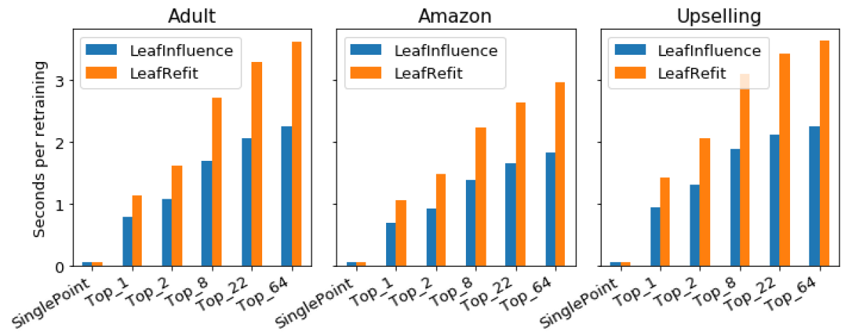
Figure 1: Wall times elapsed per training object for different variations of FastLeafRefitand FastLeafInfluence. Top_k denotes the TopKLeaves(k) update set.

Firstly, as expected, we observe that smaller update sets considerably reduce the runtimes of our algorithms, with the most radical speedup yielded by SinglePoint due to not having to recalculate any derivatives at all. Secondly, quite naturally, FastLeafInfluence performs much faster than FastLeafRefit, presumably due to vectorization and gradient precomputation (see end of Section 3.2.1). These observations confirm RQ2.

4.5 Harmful Object Removal

In this experiment, we consider a particular use-case scenario, classification in the presence of label noise, and evaluate whether our methods are able to identify training objects that are (1) noisy, (2) harmful for specific test objects . In order to do that, we randomly select $k$ training samples, flip their labels, and obtain GBDT’s predictions on test data before and after noise injection. We then conduct two experiments:

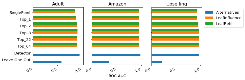
Figure 2: ROC-AUC of noise detection qualities.

(a) Logloss reduction on a particular test index.

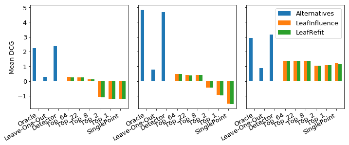
(b) Logloss reduction on the whole test set.

Figure 3: Mean DCG for relative Logloss reductions.

A. We sort the training points in ascending order of average influence on test objects and measure ROC-AUC of noise detection. In addition to variations of FastLeafRefit and FastLeafInfluence, we also compare against (1) A noise detection method exploiting the problem structure, which scores the training points using GBDT’s prediction in favor of the class opposite to its observed label (Detector), (2) actual loss changes after leave-one-out retraining (Leave-One-Out), and (3) ground-truth binary labels of the train object being noisy (Oracle) . The results are given in Fig. 2.

B. We select $n=50$ test points that suffered the largest Logloss increase, thus simulating problematic test objects. For each of these objects, we sort the training points in ascending order of influence and incrementally remove them from the training set in batches of $m=50$ objects; on each iteration we measure the relative Logloss reduction both on this given test object and on the whole test set $\mathbf{X}_{test}$ and, similarly to ranking, calculate DCG using these reductions as gains. Finally, we average these metrics over the $n$ test points. The results are given in Fig. 3(a) and 3(b).

Firstly, from Fig. 2, we note that all variations of FastLeafRefit and FastLeafInfluence perform strongly on the overall noise detection problem, where they score close to the top-performing Detector. Secondly, our methods greatly outperform their competitors (shown in blue on Fig. 3(a)) in targeting training objects harmful for a particular test object. These two observations confirm the hypothesis of RQ3. Finally, the two parts on Fig. 3 address RQ4 by clearly showing the way in which larger update sets increase quality: while all approximations score comparably in targeting particular test objects, smaller update sets lead to worsening the overall test quality (except for Upselling); in other words, smaller update sets lead to overfitting the targeted test object. Proper configurations of TopKLeaves, on the other hand, allow to “fix” a specific test object without overfitting it (k=8, 22, 64 for Adult and Amazon).

4.6 Debugging Domain Mismatch

A common issue in the supervised machine learning is domain mismatch. This is a situation, when the joint distribution of points in the test dataset $\mathbf{X}_{test}$ differs from the one in the labeled training dataset $\mathbf{X}_{train}$. Often in such scenarios, a model fine-tuned on the training dataset fails to produce accurate predictions on the test data. A standard way to cope with this problem is re-weighting $\mathbf{X}_{train}$.

In the following experiment we demonstrate that by identifying influential samples in $\mathbf{X}_{train}$ for certain subsamples in $\mathbf{X}_{test}$ we are able to detect domain mismatch and get a hint on how the distribution of points in $\mathbf{X}_{train}$ should be modified in order to match better the distribution of points in $\mathbf{X}_{test}$. The design of this experiment is a modification of the corresponding use-case of Koh & Liang (2017). We use the same Hospital dataset (see Section 4.2), with each point being a hospital patient represented by 127 features and the goal is to predict the readmission. To introduce domain mismatch we bias the distribution in the training dataset by filtering out a subsample of patients with $\mathrm{age}\in[40;50)$ and label $y=1$. Originally we had 169/1853 readmitted patients in this group and 2140/20000 overall; after we get 17/1601 in the $\mathrm{age}\in[40;50)$ group and 1988/19848 overall. Clearly, the distribution of labels in this specific age group becomes highly biased, while the proportion of positive labels in the whole dataset changes slightly (from 10.7% to 10.0%).

Training set $\mathbf{X}_{train}$ is naturally split into four parts $\{\mathbf{X}_{train}^{i}\}_{i=1}^{4}$ depending on the value of $y$ and whether $\mathrm{age}\in[40;50)$. One would expect that in the modified training dataset, samples with $\mathrm{age}\in[40;50)$ and $y=1$ are the most (positively) influential, so their removal will be the most harmful for the performance on the test dataset, while the removal of the samples with $\mathrm{age}\in[40;50)$ and $y=0$ might even be beneficial, since it is the most straightforward way to align the distributions in the test and train datasets. Below we confirm this expectation.

Let us focus on the subset $\mathbf{X}_{test}^{0}:=\{\mathbf{x}\in\mathbf{X}_{test}\,|\,\mathrm{age}(\mathbf{x})\in[40;50)\}$, since its elements are expected to be the most affected by the introduced domain mismatch. We sample 100 points from every part $\{\mathbf{X}_{train}^{i}\}_{i=1}^{4}$ (or take the whole part, if it has $<100$ points). For each of the methods FastLeafRefit and FastLeafInfluence with various update sets we compute the influence of the training samples on $\mathbf{X}_{test}^{0}$. Specifically, (a) with FastLeafRefit, for an element $\mathbf{x}\in\mathbf{X}_{train}$ we find the average Logloss reduction on $\mathbf{X}_{test}^{0}$, introduced by removing $\mathbf{x}$; (b) with FastLeafInfluence, for an element $\mathbf{x}\in\mathbf{X}_{train}$ we find the derivative of the average Logloss on $\mathbf{X}_{test}^{0}$ with respect to the weight $w$ of $\mathbf{x}$ at $w=1$.

Table 3 provides the average influence among the sampled train points with the fixed label $y\in\{0,1\}$ and the fixed indicator $I(\mathrm{age}\in[40;50))\in\{0,1\}$.

Table 3: Influence of the points in $\mathbf{X}_{train}$ on the loss on $\mathbf{X}_{test}^{0}$ averaged in the corresponding sampled group (LR=LeafRefit, LI=LeafInfluence).

	$\mathrm{age\in[40;50)}$		$\mathrm{age\not\in[40;50)}$
Method	$y=1$	$y=0$	$y=1$	$y=0$
LR SinglePoint	-0.525	0.151	0.084	0.141
LR Top1Leaves	-0.515	0.150	0.093	0.140
LR Top2Leaves	-0.489	0.150	0.103	0.139
LR Top8Leaves	-0.397	0.147	0.120	0.137
LR Top22Leaves	-0.385	0.146	0.124	0.137
LR Top64Leaves	-0.384	0.146	0.124	0.137
LI SinglePoint	-0.652	0.015	-0.052	0.005
LI Top1Leaves	-0.642	0.014	-0.043	0.004
LI Top2Leaves	-0.616	0.014	-0.033	0.003
LI Top8Leaves	-0.524	0.011	-0.015	0.001
LI Top22Leaves	-0.512	0.011	-0.012	0.001
LI Top64Leaves	-0.511	0.010	-0.011	0.001

As expected, with all methods, the samples of the same type, as the filtered samples, are consistently the most influential. Indeed, removal of these samples increases the most the loss on $\mathbf{X}_{test}$, and the derivative of the loss with respect to the weights of these samples is negative indicating that FastLeafInfluence favors upweighting them. In all cases removal of elements with $y=0$ and $\mathrm{age}\in[40;50)$ is estimated to be profitable, also confirming the initial expectations. These results allow us to answer RQ5 in the positive.

5 Conclusion

In this work, we addressed the problem of finding train objects that exerted the largest influence on the GBDT’s prediction on a particular test object. Building on the Influence Function framework for parametric models, we derived LeafRefit and LeafInfluence, methods for estimating influences based on their respective proxy metrics, Proxies 1 and 2. By utilizing the structure of tree ensembles, we also derived computationally efficient approximations to these methods, FastLeafRefit and FastLeafInfluence. In our experiments, through considering several applied scenarios, we showed the practical applicability of these approaches, as well as their ability to produce actionable insights allowing to improve the existing model.

Supplementary 1: Dataset Statistics and CatBoost Parameters

In this supplementary material, we specify the main statistics of the evaluation datasets (Table 1) and values of CatBoost parameters used in the experiments (Table 2):

Table 1: Dataset statistics.

Dataset	No. Features	Train size	Test size
Adult	14	32,561	16,281
Amazon	9	26,215	6,554
Upselling	214	35,000	15,000
Hospital	127	20,000	81,766

Table 2: Dataset CatBoost parameters.

Dataset	No. Trees	Depth	Learn rate	Formula
Adult	100	6	0.20	Newton
Amazon	100	6	0.15	Newton
Upselling	100	6	0.15	Newton

References

- dat (1996) Adult data set. https://archive.ics.uci.edu/ml/datasets/adult, 1996.
- dat (2009) Kdd cup 2009 upselling dataset. http://www.kdd.org/kdd-cup/view/kdd-cup-2009, 2009.
- dat (2013) Amazon employee access challenge dataset. https://www.kaggle.com/c/amazon-employee-access-challenge, 2013.
- cat (2018) Catboost - open-source gradient boosting library. https://catboost.yandex/, 2018.
- dcg (2018) Discounted cumulative gain. https://en.wikipedia.org/wiki/Discounted_cumulative_gain, 2018.
- Ancona et al. (2017) Ancona, Marco, Ceolini, Enea, Öztireli, Cengiz, and Gross, Markus. A unified view of gradient-based attribution methods for deep neural networks. arXiv preprint arXiv:1711.06104, 2017.
- Chen & Guestrin (2016) Chen, Tianqi and Guestrin, Carlos. Xgboost: A scalable tree boosting system. In Proceedings of the 22nd ACM SIGKDD International Conference on Knowledge Discovery and Data Mining, pp. 785–794. ACM, 2016.
- Cook & Weisberg (1980) Cook, R. Dennis and Weisberg, Sanford. Characterizations of an empirical influence function for detecting influential cases in regression. Technometrics, 22:495–508, 1980.
- Dorogush et al. (2017) Dorogush, Anna Veronika, Gulin, Andrey, Gusev, Gleb, Kazeev, Nikita, Prokhorenkova, Liudmila Ostroumova, and Vorobev, Aleksandr. Fighting biases with dynamic boosting. arXiv preprint arXiv:1706.09516, 2017.
- Fong & Vedaldi (2017) Fong, Ruth C and Vedaldi, Andrea. Interpretable explanations of black boxes by meaningful perturbation. arXiv preprint arXiv:1704.03296, 2017.
- Friedman (2001) Friedman, Jerome H. Greedy function approximation: a gradient boosting machine. Annals of statistics, pp. 1189–1232, 2001.
- Ho (1995) Ho, Tin Kam. Random decision forests. In Proceedings of the 3rd International Conference on Document Analysis and Recognition, pp. 278–282, Montreal, QC, 1995.
- Koh & Liang (2017) Koh, Pang Wei and Liang, Percy. Understanding black-box predictions via influence functions. arXiv preprint arXiv:1703.04730, 2017.
- Lundberg & Lee (2017) Lundberg, Scott M. and Lee, Su-In. Consistent feature attribution for tree ensembles. arXiv preprint arXiv:1706.06060, 2017.
- Palczewska et al. (2013) Palczewska, Anna, Palczewski, Jan, Robinson, Richard Marchese, and Neagu, Daniel. Interpreting random forest models using a feature contribution method. In Information Reuse and Integration (IRI), 2013 IEEE 14th International Conference on, pp. 112–119. IEEE, 2013.
- Quinlan (1986) Quinlan, J. Ross. Induction of decision trees. Machine learning, 1(1):81–106, 1986.
- Quinlan (2014) Quinlan, J Ross. C4. 5: programs for machine learning. Elsevier, 2014.
- Ribeiro et al. (2016) Ribeiro, Marco Tulio, Singh, Sameer, and Guestrin, Carlos. Why should I trust you?: Explaining the predictions of any classifier. In Proceedings of the 22nd ACM SIGKDD International Conference on Knowledge Discovery and Data Mining, pp. 1135–1144. ACM, 2016.
- Shrikumar et al. (2017) Shrikumar, Avanti, Greenside, Peyton, and Kundaje, Anshul. Learning important features through propagating activation differences. arXiv preprint arXiv:1704.02685, 2017.
- Strack et al. (2014) Strack, Beata, DeShazo, Jonathan P, Gennings, Chris, Olmo, Juan L, Ventura, Sebastian, Cios, Krzysztof J, and Clore, John N. Impact of hba1c measurement on hospital readmission rates: analysis of 70,000 clinical database patient records. BioMed research international, 2014, 2014.
- Sundararajan et al. (2017) Sundararajan, Mukund, Taly, Ankur, and Yan, Qiqi. Axiomatic attribution for deep networks. arXiv preprint arXiv:1703.01365, 2017.
- Tolomei et al. (2017) Tolomei, Gabriele, Silvestri, Fabrizio, Haines, Andrew, and Lalmas, Mounia. Interpretable predictions of tree-based ensembles via actionable feature tweaking. In Proceedings of the 23rd ACM SIGKDD International Conference on Knowledge Discovery and Data Mining, pp. 465–474. ACM, 2017.