Dynamical structure factor of the triangular antiferromagnet: the Schwinger boson theory beyond the mean field approach

Abstract

We compute the zero temperature dynamical structure factor $S({\bm{q}},\omega)$ of the triangular lattice Heisenberg model (TLHM) using a Schwinger boson approach that includes the Gaussian fluctuations ($1/N$ corrections) of the saddle point solution. While the ground state of this model exhibits a well-known 120^∘ magnetic ordering, experimental observations have revealed a strong quantum character of the excitation spectrum. We conjecture that this phenomenon arises from the proximity of the ground state of the TLHM to the quantum melting point separating the magnetically ordered and spin liquid states. Within this scenario, magnons are described as collective modes (two spinon-bound states) of a spinon condensate (Higgs phase) that spontaneously breaks the SU(2) symmetry of the TLHM. Crucial to our results is the proper account of this spontaneous symmetry breaking. The main qualitative difference relative to semi-classical treatments ($1/S$ expansion) is the presence of a high-energy spinon continuum extending up to about three times the single-magnon bandwidth. In addition, the magnitude of the ordered moment ($m=0.224$) agrees very well with numerical results and the low energy part of the single-magnon dispersion is in very good agreement with series expansions. Our results indicate that the Schwinger boson approach is an adequate starting point for describing the excitation spectrum of some magnetically ordered compounds that are near the quantum melting point separating this Higgs phase from the deconfined spin liquid state.

I Introduction

Novel quantum states in strongly interacting electron systems are boosting a new era of quantum materials. Tokura et al. (2017) Understanding their basic constituents is necessary to predict their behavior under different conditions and to derive low-energy theories that can describe the interplay between charge and spin degrees of freedom in doped magnets. It is then imperative to develop new approaches beyond the conventional paradigms. More specifically, the increasingly refined spectra produced by recent advances in inelastic neutron scattering Han et al. (2012); Zhou et al. (2012); Banerjee et al. (2016); Ma et al. (2016); Paddison et al. (2017); Ito et al. (2017) are demanding new theories that can account for multiple anomalies observed in dynamical spin structure factor $S({\bm{q}},\omega)$ of frustrated quantum antiferromagnets.

In the conventional paradigm, Landau (1937) magnetic order develops at low enough temperatures via spontaneous symmetry breaking. Anderson (1997) The elementary low-energy quasi-particles are spin one modes known as magnons. In the new paradigm Anderson (1973), zero-point or quantum fluctuations enhanced by magnetic frustration and/or low dimensionality may preclude conventional symmetry breaking, leading to a quantum spin liquid phase at $T=0.$ ed. by Lacroix C. (2010) Topologically ordered quantum spin liquids are different from simple quantum paramagnets because they cannot be adiabatically connected with any product state and they can support excitations with fractional quantum numbers. Wen (2002); Sachdev (2008); Normand (2009); Balents (2010); Savary and Balents (2017); Zhou et al. (2017) The first proposal of a topologically ordered quantum spin liquid was the resonant valence bond (RVB) state introduced by P. W. Anderson to describe the ground state of the TLHM. Anderson (1973) The RVB state is a linear superposition of different configurations of short range singlet pairs, whose resonant character leads to the decay of spin one modes into pairs of free $S=1/2$ spinons.

The nature of the ground state of the triangular Heisenberg antiferromagnet was a controversial topic for a long time. Zheng et al. (2006) Finally, a sequence of numerical works Huse and Elser (1988); Bernu et al. (1992); Singh and Huse (1992); Capriotti et al. (1999); White and Chernyshev (2007) provided enough evidence in favor of long range Néel magnetic order ($120^{\circ}$ ordering) with a relatively small ordered moment ($41\%$ of the full moment). Capriotti et al. (1999); Zheng et al. (2006); White and Chernyshev (2007) This sizable reduction of the ordered moment is indicative of strong quantum fluctuations and of the proximity to a quantum spin liquid phase. In a semi-classical treatment of the problem ($1/S$ expansion), the presence of strong quantum fluctuations manifests via a large $1/S$ correction of the magnon bandwidth along with single to two magnon decay in a large region of the Brillouin zone. Starykh et al. (2006); Chernyshev and Zhitomirsky (2006, 2009); Zhitomirsky and Chernyshev (2013)

Early studies of the low temperature properties based on an effective quantum field theory suggested the need of adopting alternative descriptions to the semiclassical approach. Read and Sachdev (1991); Sachdev and Read (1991); Chubukov et al. (1994) In particular, Chubukov et al. Chubukov et al. (1994) proposed that the AF triangular Heisenberg model is in the crossover region between a classical renormalized and a quantum critical regime of deconfined spinons at temperatures $T\sim 0.4J$. As shown in Fig. 1, this observation is consistent with the proximity of the $120^{\circ}$ Néel order to a zero temperature quantum melting point (QMP). If the quantum phase transition between the mangetically ordered state and the spin liquid phase turns out to be continuous (or quasi-continuous), the magnon modes should be described as weakly bounded two-spinon bound states in the proximity of the QMP. In other words, the two-spinon confinement length $\xi_{\rm conf}$ should become significantly larger than the lattice spacing ($\xi_{\rm conf}\gg a$) near the QMP. Indeed, it is known that the $J_{1}-J_{2}$ (nearest and next-nearest exchange coupling) triangular Heisenberg model exhibits a transition into a spin liquid state at $J_{2}/J_{1}\simeq 0.06$. Manuel and Ceccatto (1999); Mishmash et al. (2013); Kaneko et al. (2014); Li et al. (2015); Zhu and White (2015); Hu et al. (2015); Iqbal et al. (2016); Saadatmand and McCulloch (2016); Bauer and Fjærestad (2017); Gong et al. (2017); Zhu et al. (2018) Recent numerical studies Zhu et al. (2018) indicate that this is a continuous quantum phase transition between the $120^{\circ}$ Néel ordered state and the spin liquid phase.

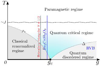
Figure 1: Schematic finite temperature phase diagram for $2D$ frustrated antiferromagnets. Coldea et al. (2003) $g$ is a generic measure of the zero point quantum fluctuations and $g_{c}$ connects continually a spiral magnetic state to quantum spin liquid state. The dashed lines indicate the crossover from the classical renormalized and the quantum disordered regimes to the quantum critical regime. The corresponding energy scales are the spin stiffness $\rho_{s}$ and the triplet excitation $\Delta$, respectively. The conjectured location of the spin-$\frac{1}{2}$ triangular Heisenberg model and the compound Ba₃CoSb₂O₉ are indicated by the vertical lines.

The above described picture is analogous to color confinement in quantum chromodynamics (QCD): hadrons are described as composite states of quarks, although quarks cannot be directly observed because they are confined by the gluon field that creates some kind of “string” between them. The analogy with a two-body problem with a linear interaction potential is an oversimplification because it does not account for the quantum nature of the gluon field: excited bound states of the linear potential (heavy hadron particles) are unstable and decay into lighter ones. Gell-Mann (1995); Greiner and Schafer (1994) A similar situation is expected for the above described quantum magnet: high-energy two-spinon bound states, corresponding to longitudinal modes, are expected to decay into multiple pairs of two-spinon bound states transforming the two-body problem of confinement into a many-body one. These processes should leave their fingerprint in the high-energy continuum of the dynamical spin susceptibility, which can be measured with inelastic neutron scattering (INS). Unlike other experimental techniques, INS can reveal the internal structure of the magnon modes. Identifying these signatures is then crucial to determine if a given compound provides a realization of this strong quantum mechanical effect.

Identifying condensed matter analogues of confined fractional particles is important for multiple reasons. In the first place, we can connect the original lattice or microscopic (high-energy) model with the effective (low-energy) field theory that is obtained in the long wavelength limit. Chubukov et al. (1994) Consequently, we can relate the parameters of the microscopic theory to the properties of the particles (such as hadron masses in the context of QCD) that emerge at low energies. The physics of spin ladders provides a simple 1D analog of this physics, Shelton et al. (1996); Lake et al. (1978) where the role of quarks is played by spinons, although there are also some obvious differences because the interaction between spinons is not usually attributed to gauge fields. In the second place, the emergence of gauge fields and fractionalized excitations in dimension higher than one could shed light on the unusual behavior of different classes of correlated electron materials in the proximity of a quantum critical point. Starykh and Reiter (1994); Powell and McKenzie (2011); Chubukov and Starykh (1995); Lee et al. (2006); Sachdev (2008); Vojta (2018)

Recent inelastic neutron scattering measurements performed in Ba₃CoSb₂O₉ Ma et al. (2016); Ito et al. (2017); Kamiya et al. (2018) –an experimental realization of a quasi-2D triangular $S=1/2$ antiferromagnet (AF)– are indeed suggesting that semi-classical approaches (large-$S$ expansion) do not reproduce several aspects of the dynamical structure factor $S({\bm{q}},\omega)$, despite the existence of magnetic long-range order. In particular, the magnon bandwidth $W$, the observed line broadening Ma et al. (2016) and, more importantly, the very unusual dispersive continuum extending up to $6W$ Ito et al. (2017) are the most salient features, which cannot be reproduced by linear spin wave theory (LSW) plus $1/S$ (LSW+$1/S$) corrections. Chernyshev and Zhitomirsky (2009); Mourigal et al. (2013) It is important to note that the easy-plane anisotropy and the finite inter-layer exchange of Ba₃CoSb₂O₉ preclude spontaneous single to two-magnon decay at the LSW+$1/S$ level,  which is obtained for the isotropic 2D Heisenberg model. Chernyshev and Zhitomirsky (2006, 2009) In other words, a low order $1/S$ expansion for the $S=1/2$ model relevant to Ba₃CoSb₂O₉ does not even anticipate strong quantum effects in this material. Then, as for the case of ${\mathrm{Cs}}_{2}\mathrm{Cu}{\mathrm{Cl}}_{4}$, Coldea et al. (2001, 2003); Isakov et al. (2005) it is natural to ask if the anomalies observed in the dynamical structure factor of Ba₃CoSb₂O₉ can be attributed to a long confinement length $\xi_{\rm conf}\gg a$ of spinons, as hypotesized in Fig. 1, and if a $1/N$ expansion ($N$ is the number of flavors of the fractional particles) can account for the observed anomalies.

The Schwinger boson (SB) theory –originally developed by Arovas and Auerbach Arovas and Auerbach (1988)– is an adequate technique to answer this question. The control parameter $N$ can be naturally introduced in the SB theory by increasing the number of flavors of the Schwinger bosons. Arovas and Auerbach (1988); Read and Sachdev (1991); Sachdev and Read (1991); Timm et al. (1998); Flint and Coleman (2009) The saddle point result becomes exact in the $N\to\infty$ limit. At this level, the system is described as a gas of non-interacting spinons and long range magnetic ordering manifests via a Bose condensation of the SBs. Hirsch and Tang (1989); Sarker et al. (1989); Chandra et al. (1990) The resulting dynamical spin structure factor, $S({\bm{q}},\omega)$, only includes a two-spinon continuum, which misses the true collective modes (magnons) of a magnetically ordered state. Auerbach and Arovas (1988); Chandra et al. (1990); Mila et al. (1991); Yoshioka and Miyazaki (1991); Sachdev (1992); Lefmann and Hedegård (1994); Mattsson (1995); Mezio et al. (2011) As we demonstrate in this work, magnons already arise at the Gaussian fluctuation level ($1/N$ corrections) as a result of the interaction with fluctuations of the emergent gauge fields. The crucial difference relative to previous formulations of this problem Arovas and Auerbach (1988) is that we compute $S({\bm{q}},\omega)$ on top of the spinon condensate (Higgs phase) that spontaneously breaks the SU(2) symmetry of the TLHM (broken symmetry ground state).

The broken symmetry spinon condensate is selected by adding an infinitesimal symmetry breaking field, $h$, which is sent to zero after taking the thermodynamic limit. The resulting local magnetization of the $120^{\circ}$ Néel ordering is $m=0.224$ which quantitatively agrees with quantum Monte Carlo (QMC) Capriotti et al. (1999) and density matrix renormalization group (DMRG) White and Chernyshev (2007) predictions. On the other hand, the excitation spectrum, revealed by $S(\bm{q},\omega)$, has a strong quantum character, which is not captured by low-order $1/S$ expansions. The low-energy magnons consist of two-spinon bound states confined by gauge fluctuations of the auxiliary fields. The good agreement with the relation dispersion predicted by series expansions Zheng et al. (2006) indicates that magnons may indeed have the composite nature predicted by the SB theory. Moreover, the resulting high-energy two-spinon continuum, which extends up to about three times the single-magnon bandwidth, may account for the first high-energy peak that is observed in Ba₃CoSb₂O₉. Ito et al. (2017) Furthermore, as we show in the next sections, the inclusion of Gaussian corrections removes other problems of the saddle point approximation, such as the spurious modes arising from unphysical density fluctuations of the bosonic field.

The article is organized as follows: in Sec. II we briefly review the Schwinger boson approach for treating AF Heisenberg models. Using the saddle point expansion, we derive the saddle point solution consisting of a spinon condensate that spontaneously breaks the SU(2) symmetry of the TLHM (Higgs phase) and the effect of Gaussian fluctuations of the auxiliary (gauge) fields on the ground state energy and the dynamical susceptibility. In Sec. III we show the main consequences of properly accounting for the spontaneous $SU(2)$ symmetry breaking. Sec. IV contains the results obtained for the TLHM, including the magnitude of the ordered moment, the dynamical structure factor, and the magnon dispersion relation along with a detailed analysis of the long wavelength limit. The physical implications of these results are discussed in Sec. V.

II Schwinger boson theory

In this section we present the path integral formulation of the Schwinger boson theory specialized for isotropic frustrated AF models whose ground states break the $SU(2)$ symmetry of the Heisenberg Hamiltonian. In particular, we consider the $S=1/2$ AF TLHM,

$${\cal H}=J\sum_{\langle{ij}\rangle}\bm{S}_{i}\cdot\bm{S}_{j},$$ (1)

whose ground state is known to exhibit 120^∘ magnetic ordering. Bernu et al. (1992); Huse and Elser (1988); Capriotti et al. (1999); White and Chernyshev (2007) We introduce the Schwinger boson representation of the spin $\bm{S}_{i}$ in terms of spin$-\frac{1}{2}$ boson operators $b_{i\sigma},$ through the relation

$$\bm{S}_{i}=\frac{1}{2}\bm{b}^{\dagger}_{i}\cdot\bm{\sigma}\cdot\bm{b}_{i},$$ (2)

where $\bm{b}^{\dagger}_{i}=\left(b^{\dagger}_{i\uparrow},b^{\dagger}_{i\downarrow}\right),$ $\bm{\sigma}=\left(\sigma^{x},\sigma^{y},\sigma^{z}\right)$ is the vector of Pauli matrices, and the bosons are subject to the number constraint,

$$\sum_{\sigma}b_{j\sigma}^{\dagger}b_{j\sigma}^{\;}=2S=1.$$ (3)

The Heisenberg interaction can be expressed as Ceccatto et al. (1993)

$${\bm{S}}_{i}\cdot{\bm{S}}_{j}=\,:\!{{B}_{ij}^{\dagger}{B}_{ij}}\!:\,-{A}_{ij}^{\dagger}{A}_{ij},$$ (4)

in terms of the SU(2) invariant bond operators

$${A}_{ij}=\frac{1}{2}\left(b_{i\uparrow}b_{j\downarrow}-b_{i\downarrow}b_{j\uparrow}\right),\;\;B_{ij}=\frac{1}{2}\left(b_{i\uparrow}b_{j\uparrow}^{\dagger}+b_{i\downarrow}b_{j\downarrow}^{\dagger}\right).$$

$A^{\dagger}_{ij}$ creates singlet states, while $B^{\dagger}_{ij}$ makes them resonate. These are the two key ingredients of the RVB theory proposed by P. W. Anderson. Anderson (1973) By using the operator identity $:\!{B}^{\dagger}_{ij}{B}_{ij}\!:\!+\!A^{\dagger}_{ij}{A}_{ij}=S^{2}$, the Heisenberg interaction was originally expressed in terms of the $A_{ij}$ operators only. Arovas and Auerbach (1988); Read and Sachdev (1991); Sachdev (1992) However, keeping the $A_{ij}$ and $B_{ij}$ operators in Eq. (4) for the saddle point approximation has two important advantages. It better accounts for non-collinear magnetic orderings, like the 120^∘ structure, that typically appear in frustrated magnets, Gazza and Ceccatto (1993); Manuel et al. (1994); Mezio et al. (2011, 2012) and it enables a proper extension from SU(2) $\simeq$ Sp(2) to Sp($N$), which is formally required to take the large $N$ limit with generators of the Lie algebra that are odd under time reversal. Flint and Coleman (2009) This two-singlet bond structure is currently used to classify quantum spin liquids based on the projective symmetry group. Wang and Vishwanath (2006); Messio et al. (2013)

The partition function for ${\cal H}$ is expressed in terms of the functional integral over coherent states: Auerbach (1994)

$$\mathcal{Z}[j]=\int D[\overline{b},b]D[\lambda]\ e^{\!-\int_{0}^{\beta}d\tau\!\left[\sum\limits_{i\sigma}\overline{b}_{i\sigma}^{\tau}\partial_{\tau}b_{i\sigma}^{\tau}+\ \mathcal{H}(\overline{b},b)\ +\mathcal{J}_{s}+\mathcal{J}_{b}\right]}\\ \times e^{-\int_{0}^{\beta}d\tau\ i\sum\limits_{i}\lambda_{i}^{\tau}\big{(}\sum\limits_{\sigma}\overline{b}_{i\sigma}^{\tau}b_{i\sigma}^{\tau}-2S\big{)}},$$ (5)

where

$$\mathcal{J}_{s}=\sum_{i}j_{i}^{\tau\mu}\ \bm{b}_{i}^{\tau\dagger}\cdot\sigma^{\mu}\cdot\bm{b}_{i}^{\tau},$$ (6)

represents the Zeeman coupling to a space ($i$) and time ($\tau$) dependent external field $j_{i}^{\tau\mu}$ ($\mu=x,y,z$), while

$$\mathcal{J}_{b}=\sum_{i}h_{i}^{\mu}\;\bm{b}_{i}^{\tau\dagger}\cdot\sigma^{\mu}\cdot\bm{b}_{i}^{\tau}$$ (7)

represents a linear coupling between the order parameter and a finite static symmetry breaking field $\bm{h}_{j}=\left(h\cos(\bm{Q}\cdot\bm{r}_{j}),h\sin(\bm{Q}\cdot\bm{r}_{j}),0\right)$ with $\bm{Q}=(\frac{2\pi}{3},\frac{2\pi}{\sqrt{3}})$, corresponding to the $120^{\circ}$ magnetic structure. The integration over the time and space dependent auxiliary field $\lambda_{i}^{\tau}$ accounts for the local constraint (3). The integration measures are $D[\overline{b},b]=\prod_{i\tau\sigma}\frac{d\bar{b}_{i\sigma}^{\tau}db_{i\sigma}^{\tau}}{2\pi i}$, and $D[\lambda]=\prod_{i\tau}\frac{d\lambda_{i}^{\tau}}{2\pi}$.

The Hamiltonian

$$\mathcal{H}=\frac{1}{2}\sum_{\langle ij\rangle}J_{ij}(\overline{A}_{ij}^{\tau}A_{ij}^{\tau}-\overline{B}_{ij}^{\tau}B_{ij}^{\tau})$$ (8)

is quartic in the complex numbers $\overline{b}$ and $b$. This terms can be decoupled into quadratic terms using a Hubbard-Stratonovich (HS) transformation that introduces auxiliary fields $\overline{W}^{A}$, $W^{A}$ and $\overline{W}^{B}$, $W^{B}$ to decouple the $\overline{A}A$ and $\overline{B}B$ terms, respectively:

$$e^{J_{ij}\overline{A}_{ij}^{\tau}A_{ij}^{\tau}} = \int D[\overline{W}^{A}\!,\!W^{A}]\ e^{-J_{ij}\overline{W}_{ij}^{A\tau}W_{ij}^{A\tau}}\times$$

$$\;\;\;\;\;\;\;\;\;\;\;\;\times\;e^{J_{ij}\left(\overline{W}_{ij}^{A\tau}A_{ij}^{\tau}+W_{ij}^{A\tau}\overline{A}_{ij}^{\tau}\right)},$$

and

$$e^{-J_{ij}\overline{B}_{ij}^{\tau}B_{ij}^{\tau}} = \int D[\overline{W}^{B}\!,\!W^{B}]\ e^{-J_{ij}\overline{W}_{ij}^{B\tau}W_{ij}^{B\tau}}\times$$

$$\;\;\;\;\;\;\;\;\;\;\;\;\times\;e^{J_{ij}\left(-\overline{W}_{ij}^{B\tau}B_{ij}^{\tau}+W_{ij}^{B\tau}\overline{B}_{ij}^{\tau}\right)},$$

with integration measure $D[\overline{W}^{r}\!,\!W^{r}]=\prod_{ij\tau}\frac{d\overline{W}_{ij}^{r\tau}dW_{ij}^{r\tau}}{2\pi i/J_{ij}}$, and $r=A,B$. After replacing Eqs. (II) and (II) in Eq. (5), the Gaussian integrals over $\overline{b}$ and $b$ can be formally carried out. The resulting partition function becomes

$$\mathcal{Z}[j]=\int D[\overline{W},W]D[\lambda]\ e^{-S_{\rm eff}(\overline{W},W,\lambda,j)},$$ (11)

where the effective action can be split into two terms,

$$S_{\rm eff}(\overline{W},W,\lambda,j)=S_{0}(\overline{W},W,\lambda)+S_{\rm bos}(\overline{W},W,\lambda,j),$$ (12)

with

$$S_{0}(\overline{W},W,\lambda)\!=\!\int_{0}^{\beta}d\tau\sum\limits_{ijr}J_{ij}\overline{W}_{ij}^{r\tau}W_{ij}^{r\tau}\!-\!2Si\sum_{i}\lambda_{i}^{\tau},$$ (13)

and

$$S_{\rm bos}(\overline{W},W,\lambda,j) \!=\! \frac{1}{2}\operatorname{Tr}\ln\left[\mathcal{G}^{-1}(\overline{W},W,\lambda,j)\right]=$$

$$\!=\! -\frac{1}{2}\ln\ \mathcal{Z}_{\rm bos}(\overline{W},W,\lambda,j).$$

$\overline{W}$ and $W$ are the HS fields $W_{ij}^{r\tau}$, $\overline{W}_{ij}^{r\tau}$ ($r=A,B$) and $\mathcal{G}^{-1}=\mathcal{M}$ is the bosonic dynamical matrix with the trace taken over space, time, and boson flavor indices. The bosonic partition function $\mathcal{Z}_{\rm bos}$ can be formally integrated out to get

$$\mathcal{Z}_{\rm bos}(\overline{W},W,\lambda,j)\!\! = \!\!\!\int\!D[\overline{b},b]e^{-\vec{b}^{\dagger}\cdot\mathcal{G}^{-1}(\overline{W},W,\lambda,j)\cdot\vec{b}}=$$

$$= \det\left[\mathcal{G}(\overline{W},W,\lambda,j)\right],$$

where $\vec{b}$ is a vector containing all the variables $b_{i\sigma}^{\tau}$.

The effective action (12) is invariant under the $U(1)$ gauge transformation $b_{i\sigma}^{\tau}\rightarrow b_{i\sigma}^{\tau}e^{i\theta^{\tau}_{i}}$ if the auxiliary fields transform as

$$W_{ij}^{r\tau} \rightarrow W_{ij}^{r\tau}e^{i(\theta^{\tau}_{i}\pm\theta^{\tau}_{j})},$$

$$\overline{W}_{ij}^{r\tau} \rightarrow \overline{W}_{ij}^{r\tau}e^{-i(\theta^{\tau}_{i}\pm\theta^{\tau}_{j})},$$ (15)

$$\lambda_{\bm{i}}^{\tau} \rightarrow \lambda_{\bm{i}}^{\tau}-\partial_{\tau}\theta^{\tau}_{i},$$

where the $+$ and $-$ signs hold for the $A$ and $B$ fields respectively. In other words, the phase fluctuations of the auxiliary fields represent the emergent gauge fluctuations of the SB theory.

The Fourier transformation to Matsubara frequency and momentum space is done using

$$f^{\tau}_{i}=\frac{1}{\sqrt{N_{s}\beta}}\sum_{\bm{k},i\omega_{n}}f_{\bm{k}}^{i\omega_{n}}e^{-i({\bm{k}}\cdot\bm{r}_{i}-\omega_{n}\tau)}$$ (16)

for any field $f^{\tau}_{i}$, where $i\omega_{n}=2\pi in/\beta$ are the bosonic Matsubara frequencies and $\bm{k}$ the momenta. For convenience, in what follows, we denote $f_{\bm{k}}^{i\omega_{n}}$ as $f_{\bm{k}}^{\omega}$. For simplicity, we perform a rotation to a local reference frame such that the magnetic ordering, and consequently ${\bm{h}}$, become spatially uniform. In this case the bosonic variables transform as $b_{\bm{k}\uparrow}^{\omega}\rightarrow b_{\bm{k}+\frac{\bm{Q}}{2}\uparrow}^{\omega}$ and $b_{\bm{k}\downarrow}^{\omega}\rightarrow b_{\bm{k}-\frac{\bm{Q}}{2}\downarrow}^{\omega}$. After introducing the representation $\vec{b}_{\bm{k},\omega}^{\dagger}=\left(\bar{b}_{\bm{k}\uparrow}^{\omega},b_{-\bm{k}\downarrow}^{-\omega},\overline{b}_{\bm{k}\downarrow}^{\omega},b_{-\bm{k}\uparrow}^{-\omega}\right)$, $\mathcal{G}^{-1}$ is

$$\mathcal{G}_{\bm{k,k^{\prime}}}^{-1\ \omega,\omega^{\prime}}=\left(\begin{array}[]{cccc}F_{\bm{Q}}^{B}(\bm{k,k^{\prime}},i\omega)&F_{\bm{Q}}^{A}(\bm{k,k^{\prime}})&-\frac{h}{2}\delta_{\bm{k,k^{\prime}}}&0\\ \\ \overline{F}_{\bm{Q}}^{A}(\bm{k^{\prime},k})&F_{\bm{Q}}^{B}(\bm{k^{\prime},k},-i\omega)&0&-\frac{h}{2}\delta_{\bm{k,k^{\prime}}}\\ \\ -\frac{h}{2}\delta_{\bm{k,k^{\prime}}}&0&F_{-\bm{Q}}^{B}(\bm{k,k^{\prime}},i\omega)&-F_{-\bm{Q}}^{A}(\bm{k,k^{\prime}})\\ \\ 0&-\frac{h}{2}\delta_{\bm{k,k^{\prime}}}&-\overline{F}_{-\bm{Q}}^{A}(\bm{k^{\prime},k})&F_{-\bm{Q}}^{B}(\bm{k^{\prime},k},-i\omega)\end{array}\right),$$ (17)

with matrix elements

$$F_{\bm{Q}}^{B}(\bm{k,k^{\prime}},i\omega)=\frac{1}{2}i\omega\ \delta_{\bm{k,k^{\prime}}}\delta_{\omega,\omega^{\prime}}+\frac{i\lambda_{k-k^{\prime}}^{\omega-\omega^{\prime}}}{2\sqrt{N_{s}\beta}}-\sum_{\delta>0}\frac{J_{\delta}}{4\sqrt{N_{s}\beta}}\left(W_{\bm{k-k^{\prime}},\delta}^{B\ \omega-\omega^{\prime}}e^{-i(\bm{k}^{\prime}+\frac{\bm{Q}}{2})\cdot\bm{\delta}}-\overline{W}_{\bm{k^{\prime}-k},\delta}^{B\ \omega^{\prime}-\omega}e^{i(\bm{k}+\frac{\bm{Q}}{2})\cdot\bm{\delta}}\right)\ ,$$ (18)

and

$$F_{\bm{Q}}^{A}(\bm{k,k^{\prime}})=\sum_{\delta>0}\frac{J_{\delta}}{4\sqrt{N_{s}\beta}}W_{\bm{k-k^{\prime}},\delta}^{A\ \omega-\omega^{\prime}}\left(e^{i(\bm{k}+\frac{\bm{Q}}{2})\cdot\bm{\delta}}-e^{-i(\bm{k}^{\prime}+\frac{\bm{Q}}{2})\cdot\bm{\delta}}\right)\ ,$$ (19)

where $\bm{\delta}$ represents (half of) the vectors connecting the nearest neighours of the triangular lattice.

II.1 The saddle point expansion

To evaluate Eq. (11) we expand the effective action $S_{\rm eff}$ about its saddle point, Auerbach (1994) defined by the set of saddle point equations

$$\frac{\partial S_{\rm eff}}{\partial\phi_{\alpha}}\bigg{|}_{\rm sp}=\frac{\partial\ S_{0}}{\partial\phi_{\alpha}}\bigg{|}_{\rm sp}+\frac{1}{2}\operatorname{Tr}\bigg{[}\mathcal{G}^{\rm sp}\frac{\partial\mathcal{G}^{-1}}{\partial\phi_{\alpha}}\bigg{]}=0,$$ (20)

where $\phi_{\alpha}$ denotes the fields $\left\{\overline{W}_{\bm{k},\delta}^{r\omega},\ W_{\bm{k},\delta}^{r\omega},\ \lambda_{\bm{k}}^{\omega}\right\}$ ($\alpha$ includes field, momentum, and frequency indices). The expansion of the effective action becomes

$$S_{\rm eff}=S^{\rm sp}_{\rm eff}+\sum_{\alpha_{1}\alpha_{2}}S_{\alpha_{1}\alpha_{2}}^{(2)}\ \Delta\phi_{\alpha_{1}}\Delta\phi_{\alpha_{2}}+S_{int},$$ (21)

where $S^{\rm sp}_{\rm eff}$ corresponds to the effective action evaluated at the saddle point fields $\phi_{\alpha}^{\rm sp}$, the second term takes into account the auxiliary field fluctuations $\Delta\phi_{\alpha}=\phi_{\alpha}-\phi_{\alpha}^{\rm sp}$ at the Gaussian level, and the last term $S_{int}=\sum_{n=3}^{\infty}\sum_{\alpha_{1}\cdots\alpha_{n}}S_{\alpha_{1}\cdots\alpha_{n}}^{(n)}\ \Delta\phi_{\alpha_{1}}\cdots\Delta\phi_{\alpha_{n}}$ includes auxiliary field fluctuations of third and higher orders. The coefficients are defined as

$$S_{\alpha_{1}\cdots\alpha_{n}}^{(n)}=\frac{1}{n!}\left.\frac{\partial^{n}S_{\rm eff}}{\partial\phi_{\alpha_{1}}\cdots\ \partial\phi_{\alpha_{n}}}\right|_{\rm sp},$$ (22)

for $n\geq 2$. The corresponding partition function (11) is

$$\mathcal{Z}[j]=e^{-S^{\rm sp}_{\rm eff}{(\overline{W}_{\rm sp},{W}_{\rm sp},\lambda_{\rm sp},j)}}\times\int D[\bar{\phi},\phi]\ e^{-\Delta\vec{\phi}^{\dagger}\cdot S^{(2)}\cdot\Delta\vec{\phi}+S_{int}}.$$

The first factor represents the partition function within the saddle point approximation, while the second one is the contribution from the fluctuations of the auxiliary fields: $\Delta\vec{\phi}^{\dagger}=\vec{\phi}^{\dagger}-\vec{\phi}^{{\rm sp}\dagger}$ with $\vec{\phi}^{\dagger}=\left(\overline{W}_{\bm{k},\delta}^{r\omega},\ W_{-\bm{k},\delta}^{r-\omega},\ \lambda_{-\bm{k}}^{-\omega}\right)$.

II.1.1 Saddle Point Approximation

For a static and homogeneous saddle point solution, the Fourier transformed fields satisfy $\left.\phi_{\bm{k}}^{\omega}\right|_{\rm sp}=\sqrt{N_{s}\beta}\;\phi\;\delta_{\bm{k,0}}\delta_{\omega,0}$, for $\phi=\overline{W}_{\delta}^{r},W_{\delta}^{r},\lambda$. We consider the ansatz

$$W_{\delta}^{A}\big{|}_{\rm sp}=iA_{\delta}, \ \overline{W}_{\delta}^{A}\big{|}_{\rm sp}=-iA_{\delta},$$

$$W_{\delta}^{B}\big{|}_{\rm sp}=-B_{\delta}, \ \overline{W}_{\delta}^{B}\big{|}_{\rm sp}=B_{\delta}\ ,$$ (23)

$$\lambda|_{\rm sp} = i\lambda,$$

with $A_{\delta}$, $B_{\delta}$, and $\lambda$ real, which is consistent with magnetic ordering in the $xy$ plane. Ghioldi et al. (2015) While $\overline{W}_{\delta}^{A}|_{\rm sp}=(W_{\delta}^{A}|_{\rm sp})^{*}$, it turns out that $(W_{\delta}^{B}|_{\rm sp})^{*}=-\overline{W}_{\delta}^{B}|_{\rm sp}$. Trumper et al. (1997); Flint and Coleman (2009) This corresponds to a distorted saddle point solution as a consequence of the sign difference between the $\overline{W}^{A}A$ and $\overline{W}^{B}B$ terms in the HS decouplings of Eqs. (II) and  (II). Furthermore, the real field $\lambda^{\tau}_{i}$ takes an imaginary value at the SP. To reach this distorted saddle point, it is necessary to perform an analytical continuation for computing the partition function. Auerbach (1994) The resulting effective saddle point action describes a system of non-interacting bosons coupled with the static and homogeneous SP auxiliary fields:

$$S_{\rm eff}^{\rm sp}(\overline{W}_{\rm sp},W_{\rm sp},\lambda_{\rm sp})=-N_{s}\beta\sum\limits_{\delta>0}J_{\delta}\left(B_{\delta}^{2}-A_{\delta}^{2}\right)-2SN_{s}\beta\lambda-\ln\mathcal{Z}_{\rm bos}^{\rm sp},$$ (24)

where $\mathcal{Z}_{\rm bos}^{\rm sp}=\int d[\bar{b},b]\ e^{-S_{\rm bos}^{\rm sp}}$, $S_{\rm bos}^{\rm sp}=\sum_{\bm{k},\omega}\vec{b}_{\bm{k},\omega}^{\dagger}\cdot\mathcal{M}_{\bm{k},\omega}^{\rm sp}\cdot\vec{b}_{\bm{k},\omega}$ and $\mathcal{M}^{\rm sp}$ is the dynamical matrix of the bosons evaluated at the saddle point solution,

$$\mathcal{M}_{\bm{k},\omega}^{\rm sp}={\left(\begin{array}[]{cccc}(i\omega+\lambda+\gamma_{\bm{k+\frac{Q}{2}}}^{B})e^{-i\omega\eta}&-\gamma_{\bm{k+\frac{Q}{2}}}^{A}&-\frac{h}{2}&0\\ \\ -\gamma_{\bm{k+\frac{Q}{2}}}^{A}&(-i\omega+\lambda+\gamma_{\bm{k+\frac{Q}{2}}}^{B})e^{i\omega\eta}&0&-\frac{h}{2}\\ \\ -\frac{h}{2}&0&(i\omega+\lambda+\gamma_{\bm{-k+\frac{Q}{2}}}^{B})e^{-i\omega\eta}&-\gamma_{\bm{-k+\frac{Q}{2}}}^{A}\\ \\ 0&-\frac{h}{2}&-\gamma_{\bm{-k+\frac{Q}{2}}}^{A}&(-i\omega+\lambda+\gamma_{\bm{-k+\frac{Q}{2}}}^{B})e^{i\omega\eta}\end{array}\right)}\ ,$$ (25)

with

$$\gamma_{\bm{k}}^{A} = \sum\limits_{\delta>0}J_{\delta}A_{\delta}\sin\left(\bm{k\cdot\delta}\right),$$ (26)

$$\gamma_{\bm{k}}^{B} = \sum\limits_{\delta>0}J_{\delta}B_{\delta}\cos\left(\bm{k\cdot\delta}\right).$$ (27)

The convergence factors $e^{\pm i\omega\eta}$ with $\eta=0^{+}$ arise from the time ordering of the functional integral and they are crucial for the Matsubara frequency sum in Eq. (20) to be well defined. Timm et al. (1998)

The single spinon Green’s function is obtained by computing $\mathcal{G}^{\rm sp}=(\mathcal{M}^{\rm sp})^{-1}$,

$$\mathcal{G}^{\rm sp}(\bm{k},i\omega)=\sum_{\sigma}\frac{g_{\bm{k}}^{-\sigma}}{i\omega-\varepsilon_{\bm{k}\sigma}}\!+\!\frac{g_{\bm{k}}^{+\sigma}}{i\omega+\varepsilon_{\bm{k}\sigma}}\ ,$$ (28)

($\sigma=\pm$) where the two band spinon relation dispersion are

$$\varepsilon_{\bm{k}\sigma}=\sqrt{\frac{1}{2}\left[\left(\alpha_{\bm{k+\frac{Q}{2}}}^{2}+\alpha_{\bm{-k+\frac{Q}{2}}}^{2}+\frac{h^{2}}{2}\right)+\sigma\Delta_{\bm{k}}^{2}\right]}\ ,$$ (29)

with $\alpha_{\bm{k}}^{2}=\left(\lambda+\gamma_{\bm{k}}^{B}\right)^{2}-\left(\gamma_{\bm{k}}^{A}\right)^{2},$ and

$$\Delta_{\bm{k}}^{2}=\sqrt{\Big{(}\alpha_{\bm{k+\frac{Q}{2}}}^{2}-\alpha_{\bm{-k+\frac{Q}{2}}}^{2}\Big{)}^{2}+\bigg{[}\Big{(}(\lambda+\gamma_{\bm{k+\frac{Q}{2}}}^{B})+(\lambda+\gamma_{\bm{-k+\frac{Q}{2}}}^{B})\Big{)}^{2}-\Big{(}\gamma_{\bm{k+\frac{Q}{2}}}^{A}-\gamma_{\bm{-k+\frac{Q}{2}}}^{A}\Big{)}^{2}\bigg{]}\;h^{2}}.$$ (30)

The $4\times 4$ matrices $g_{\bm{k}}^{\pm\;\sigma}$ are

$$g_{\bm{k}}^{+\;\sigma}=\left(\begin{array}[]{cccc}E_{\bm{k}\sigma}&C_{\bm{k}\sigma}&F_{\bm{k}\sigma}&D_{-\bm{k}\sigma}\\ C_{\bm{k}\sigma}&A_{\bm{k}\sigma}&D_{\bm{k}\sigma}&B_{\bm{k}\sigma}\\ F_{\bm{k}\sigma}&D_{\bm{k}\sigma}&E_{-\bm{k}\sigma}&C_{-\bm{k}\sigma}\\ D_{-\bm{k}\sigma}&B_{\bm{k}\sigma}&C_{-\bm{k}\sigma}&A_{-\bm{k}\sigma}\\ \end{array}\right)\ \quad g_{\bm{k}}^{-\;\sigma}=-\left(\begin{array}[]{cccc}A_{\bm{k}\sigma}&C_{\bm{k}\sigma}&B_{\bm{k}\sigma}&D_{\bm{k}\sigma}\\ C_{\bm{k}\sigma}&E_{\bm{k}\sigma}&D_{-\bm{k}\sigma}&F_{\bm{k}\sigma}\\ B_{\bm{k}\sigma}&D_{-\bm{k}\sigma}&A_{-\bm{k}\sigma}&C_{-\bm{k}\sigma}\\ D_{\bm{k}\sigma}&F_{\bm{k}\sigma}&C_{-\bm{k}\sigma}&E_{-\bm{k}\sigma}\\ \end{array}\right),$$ (31)

with matrix elements

$$A_{\bm{k}\sigma}=v_{\bm{k}\sigma}^{2}\frac{\Delta_{-\bm{k}\sigma}^{2}}{\Delta_{\bm{k}}^{2}}+\sigma u_{-{\bm{k}\sigma}}^{2}\frac{h^{2}}{4\Delta_{\bm{k}}^{2}},\qquad E_{\bm{k}\sigma}=u_{\bm{k}\sigma}^{2}\frac{\Delta_{-\bm{k}\sigma}^{2}}{\Delta_{\bm{k}}^{2}}+\sigma v_{-\bm{k}\sigma}^{2}\frac{h^{2}}{4\Delta_{\bm{k}}^{2}},\qquad C_{\bm{k}\sigma}=z_{\bm{k}\sigma}\frac{\Delta_{-\bm{k}\sigma}^{2}}{\Delta_{\bm{k}}^{2}}-\sigma z_{-\bm{k}\sigma}\frac{h^{2}}{4\Delta_{\bm{k}}^{2}},$$ (32)

$$B_{\bm{k}\sigma}=-\sigma\varepsilon_{\bm{k}\sigma}\left[v_{\bm{k}\sigma}^{2}v_{-\bm{k}\sigma}^{2}+z_{\bm{k}\sigma}z_{-\bm{k}\sigma}-\left(\frac{h}{4\varepsilon_{\bm{k}\sigma}}\right)^{2}\right]\frac{h}{\Delta_{\bm{k}}^{2}}\ ,\quad F_{\bm{k}\sigma}=-\sigma\varepsilon_{\bm{k}\sigma}\left[u_{\bm{k}\sigma}^{2}u_{-\bm{k}\sigma}^{2}+z_{\bm{k}\sigma}z_{-\bm{k}\sigma}-\left(\frac{h}{4\varepsilon_{\bm{k}\sigma}}\right)^{2}\right]\frac{h}{\Delta_{\bm{k}}^{2}}\ ,\quad$$ (33)

and

$$D_{\bm{k}\sigma}=-\sigma\varepsilon_{\bm{k}\sigma}\left[v_{\bm{k}\sigma}^{2}z_{-\bm{k}\sigma}+u_{-\bm{k}\sigma}^{2}z_{\bm{k}\sigma}\right]\frac{h}{2\Delta_{\bm{k}}^{2}}\ ,$$ (34)

where

$$u_{\bm{k}\sigma}^{2}=\frac{\lambda+\gamma_{\scriptscriptstyle{\bm{k+\frac{Q}{2}}}}^{B}}{2\varepsilon_{\bm{k}\sigma}}+\frac{1}{2}\ ,\qquad v_{\bm{k}\sigma}^{2}=\frac{\lambda+\gamma_{\scriptscriptstyle{\bm{k+\frac{Q}{2}}}}^{B}}{2\varepsilon_{\bm{k}\sigma}}-\frac{1}{2}\ ,$$ (35)

$$z_{\bm{k}\sigma}=\frac{\gamma_{\scriptscriptstyle{\bm{k+\frac{Q}{2}}}}^{A}}{2\varepsilon_{\bm{k}\sigma}}\ ,\qquad\Delta_{\bm{k}\sigma}^{2}=\sigma\left(\varepsilon_{\bm{k}\sigma}^{2}-\alpha_{\bm{k+\frac{Q}{2}}}^{{2}}\right)\ .$$ (36)

By replacing the Green’s functions and the dynamical matrix given in Eqs. (28) and (25), respectively, the saddle point condition Eq. (20) at $T=0$, yields the following self-consistent equations for the mean field parameters $A_{\delta}$, $B_{\delta}$, and $\lambda$,

$$A_{\delta} = \frac{1}{N_{s}}\sum_{\bm{k}\sigma}C_{\bm{k}\sigma}\sin\left(\bm{k}+\frac{\bm{Q}}{2}\right)\cdot\bm{\delta},$$

$$B_{\delta} = \frac{1}{N_{s}}\sum_{\bm{k}\sigma}A_{\bm{k}\sigma}\cos\left(\bm{k}+\frac{\bm{Q}}{2}\right)\cdot\bm{\delta},$$ (37)

$$S\ = \frac{1}{N_{s}}\sum_{\bm{k}\sigma}A_{{\bf k}\sigma}.\qquad\qquad\quad\quad$$

These equations coincide with the Schwinger boson mean field theory (SBMFT). In particular, the usual system of equations for a singlet ground state is recovered for $h=0$, Mezio et al. (2011)

$$A_{\delta} = \frac{1}{N_{s}}\sum_{\bm{k}}\frac{\gamma_{\bm{k}}^{A}}{2\alpha_{\bm{k}}}\sin(\bm{k\cdot\delta}),$$

$$B_{\delta} = \frac{1}{N_{s}}\sum_{\bm{k}}\frac{\lambda+\gamma_{\bm{k}}^{B}}{2\alpha_{\bm{k}}}\cos(\bm{k\cdot\delta}),$$ (38)

$$S+\frac{1}{2} = \frac{1}{N_{s}}\sum_{\bm{k}}\frac{\lambda+\gamma_{\bm{k}}^{B}}{2\alpha_{\bm{k}}},$$

where $\alpha_{\bm{k}}$ is the spinon dispersion relation in a global reference frame for $h=0$.

II.1.2 Gaussian fluctuation approximation

The $S_{int}$ term of Eq. (21) is neglected within the Gaussian fluctuation approximation, so as to keep the field fluctuations in the effective action up to quadratic order,

$$S_{\rm eff}\simeq S^{\rm sp}_{\rm eff}+\sum_{\alpha_{1}\alpha_{2}}\Delta\vec{\phi}_{\alpha_{1}}^{\dagger}\cdot S_{\alpha_{1}\alpha_{2}}^{(2)}\cdot\Delta\vec{\phi}_{\alpha_{2}}\ .$$ (39)

The coefficients of the quadratic terms $S^{(2)}$ define the fluctuations matrix

$$S_{\alpha_{1}\alpha_{2}}^{(2)}\!\!\! = \frac{1}{2}\ \frac{\partial^{2}S_{\rm eff}}{\partial\phi_{\alpha_{1}}\partial\phi_{\alpha_{2}}}\bigg{|}_{\rm sp}=$$

$$= \frac{1}{2}\ \Bigg{\{}\frac{\partial^{2}S_{0}}{\partial\phi_{\alpha_{1}}\partial\phi_{\alpha_{2}}}-\frac{1}{2}\operatorname{Tr}\Big{[}\mathcal{G}^{\rm sp}\ v_{\phi_{\alpha_{1}}}\ \mathcal{G}^{\rm sp}\ v_{\phi_{\alpha_{2}}}\Big{]}\Bigg{\}}\equiv$$

$$\equiv \Big{(}\Pi_{0}-\Pi\Big{)}_{\alpha_{1}\alpha_{2}}.$$

$\Pi_{0}$ is a diagonal matrix containing the coupling constant $J_{\bm{\delta}}$ in the diagonal, and a zero in the $\lambda\lambda$ element, $\Pi$ is the so-called polarization matrix, and $v_{\phi}=\frac{\partial\mathcal{G}^{-1}}{\partial\phi}$ are the internal vertices, i. e., the derivatives of the bosonic dynamical matrix with respect to the auxiliary fields. Auerbach (1994)

The distorted character of the SP has two important consequences. The first one is the need to perform an analytic continuation of the real and the imaginary parts of the auxiliary fields in the Gaussian integral

$$\int D[\bar{\phi},\phi]\ e^{-\Delta\vec{\phi}^{\dagger}\cdot S^{(2)}\cdot\Delta\vec{\phi}},$$ (41)

in order to pass through the SP. The second one is the non-Hermiticity of the fluctuation matrix.

Regarding the first issue, the analytical continuation leads to a $\Delta\vec{\phi}^{\dagger}=\vec{\phi}^{\dagger}-\vec{\phi}^{{\rm sp}\dagger}$ in Eq. (41) that is not necessarily the Hermitian conjugated of $\Delta\vec{\phi}$. One way to circumvent this problem in the evaluation of the Gaussian integral is to make a simple change of integration variables, $\Delta\vec{\phi}\to\vec{\phi}$, consisting of the rigid shifts of the real and the imaginary parts of the auxiliary field axes, so that the SP is shifted to the origin of the integration domain and, hence, $\vec{\phi}^{\dagger}$ and $\vec{\phi}$ become conjugate variables. In fact, as the integrand is an analytical function of the real and imaginary parts of the auxiliary fields, this change of variables can be seen as a “rectangular” deformation of the real and imaginary parts of the auxiliary field axes.

On the other hand, due to the non-Hermiticity of the fluctuation matrix, the stability of the Gaussian fluctuations about the SP must be analized carefully. In particular, the convergence of the Gaussian integral $\int D[\bar{\phi},\phi]e^{-\vec{\phi}^{\dagger}\cdot S^{(2)}\cdot\vec{\phi}},$ is given by the positive-stable condition of the fluctuation matrix (see Appendix A). A matrix is positive-stable if all of its eigenvalues have a positive real part. This condition is less restrictive than the usual requirement of positive-definiteness of the Hermitian part of the matrix. Negele and Orland (1998) In fact, in our case we have found that for the TLHM the fluctuation matrix is always positive-stable while its Hermitian part is indefinite.

It is worth mentioning that, if the positive-stable condition is satisfied, the Gaussian integral (41) can be evaluated alternatively through the steepest descent method. Auerbach (1994) In this method, the real and imaginary parts of the auxiliary field axes are deformed such that the integrand, along the deformed path, has a constant phase close to the SP. Mathematically, the expected optimal direction of the path is obtained from the singular value decomposition (SVD) of the fluctuation matrix:

$$S^{(2)}=U\cdot\Sigma\cdot V^{\dagger},$$ (42)

where $U,V$ are complex unitary matrices and $\Sigma=\text{diag}[s_{1},...,s_{n}]$ is a semi-positive definite diagonal matrix with $n\times n$ being the dimension of the fluctuation matrix. The steepest descent path is then given by

$$\vec{\phi}^{\dagger}=\vec{\phi}^{H}\cdot V\cdot U^{\dagger},$$ (43)

where the superscript $H$ denotes the Hermitian conjugate of $\vec{\phi}$. Notice that along the steepest descent path $\vec{\phi}^{\dagger}$ and $\vec{\phi}$ may not be conjugate variables. Substituting Eq. (43) into the Gaussian effective action yields

$$S_{\rm eff}\simeq S^{\rm sp}_{\rm eff}+\sum_{\alpha_{1}\alpha_{2}}\Delta\vec{\phi}_{\alpha_{1}}^{H}\cdot\tilde{S}_{\alpha_{1}\alpha_{2}}^{(2)}\cdot\Delta\vec{\phi}_{\alpha_{2}}\ .$$ (44)

with $\tilde{S}^{(2)}=V\cdot\Sigma\cdot V^{\dagger},$ which is Hermitian and semi-positive definite. So, this reformulation allows us to work with, both, a pair of conjugate variables, $\Delta\vec{\phi}^{H}$ and $\Delta\vec{\phi}$, and a Hermitian fluctuation matrix. However, it should be stressed that the stability of the Gaussian fluctuation approximation is given by the positive-stable condition of the original $S^{(2)}$ fluctuation matrix. In our case of the TLHM we have checked that the two procedures mentioned above, using non-Hermitian and Hermitian fluctuation matrices, give always the same quantitative results.

II.2 Ground state energy

In this subsection we calculate the ground state energy within the Gaussian fluctuation approximation aiming to the evaluation of the local magnetization. For this purpose we must compute the partition function at the Gaussian level with a finite symmetry breaking field $h$ (and $\mathcal{J}_{s}$ switched off). The partition function is given by

$$\mathcal{Z}^{(2)}(h)=e^{-S_{\rm eff}^{\rm sp}}\times\int D[\vec{\phi}^{\dagger},\vec{\phi}]\ e^{-\vec{\phi}^{\dagger}\cdot S^{(2)}\cdot\vec{\phi}}.$$ (45)

Within the SP approximation, the ground state energy is obtained by taking the limit $T\to 0$ of $F^{\rm sp}=S^{\rm sp}_{\rm eff}/\beta$. However, to get the correct zero point energy one should mantain the discrete character of the imaginary time $\tau$ (a very tedious procedure) to respect the correct equal-time ordering in the path integral. Alternatively, one can keep track of this time ordering by transforming the conjugate bosonic field as $\overline{b}_{\bm{k}}^{\omega}\to\overline{b}_{\bm{k}}^{\omega}e^{-i\omega\eta}$, with the convergence factor $\eta$ mentioned previously. In this case the ground state energy (per site) turns out to be

$$E^{\rm sp}_{\rm gs}(h) = \frac{1}{2N_{s}}\sum_{\bm{k}\sigma}\varepsilon_{\bm{k}\sigma}(h)-$$

$$- \sum_{\delta>0}J_{\delta}\left(B^{2}_{\delta}-A^{2}_{\delta}\right)-\lambda\left(2S+1\right),$$

which is identical to the ground state energy derived within the canonical mean field approximation. Auerbach (1994); Mezio et al. (2011)

Hereafter, we proceed to compute the Gaussian correction to the ground state energy. We use the original non-Hermitian fluctuation matrix $S^{(2)}$ and the Gaussian integral in Eq. (45) yields, for a positive-stable matrix (see Appendix A),

$$\mathcal{Z}^{\rm fl}(h)\equiv\int D[\vec{\phi}^{\dagger},\vec{\phi}]\ e^{-\vec{\phi}^{\dagger}\cdot S^{(2)}\cdot\vec{\phi}}=\frac{1}{{\rm det}\;S^{(2)}}.$$ (47)

Because of the redundant local $U(1)$ gauge degree of freedom introduced by the Schwinger boson representation [see Eq. (15)], the fluctuation matrix contains infinite zero gauge modes (one for each $\omega$ and ${\bm{k}}$ value), corresponding to the null space of $S^{(2)}$. The artificial infinities arising from these zero gauge modes are avoided by integrating only over the genuine physical fluctuations (fluctuations with restoring force). This is formally done following the Faddeev-Popov prescription. Trumper et al. (1997)

By applying an infinitesimal gauge transformation to the auxiliary fields, $\vec{\phi}\to\vec{\phi}(\theta)$, the gauge fluctuations around the saddle point solution, $\vec{\phi}^{\rm sp}(\theta)=\vec{\phi}^{\rm sp}+\delta\vec{\phi}^{\rm sp}(\theta)$, take the form

$$\delta\vec{\phi}^{\rm sp}(\theta)=\left(\begin{array}[]{c}\delta W_{\bm{k},\delta}^{r\ \omega}(\theta)\\ \delta\overline{W}_{-\bm{k},\delta}^{r\ -\omega}(\theta)\\ \delta\lambda_{\bm{k}}^{\omega}(\theta)\\ \end{array}\right),$$ (48)

where

$$\delta W_{\bm{k},\delta}^{r\;\omega}(\theta) = i(1\pm e^{i\bm{k}\cdot\bm{\delta}})\left.{W_{\delta}}^{r}\right|_{\rm sp}\theta_{{\bm{k}}\omega},$$

$$\delta\overline{W}_{-\bm{k},\delta}^{r\;-\omega}(\theta) = -i(1\pm e^{i\bm{k}\cdot\bm{\delta}})\left.\overline{W}_{\delta}^{r}\right|_{\rm sp}\theta_{{\bm{k}}\omega},$$ (49)

$$\delta\lambda_{\bm{k}}^{\omega}(\theta) = -i\omega_{n}\theta_{{\bm{k}}\omega}.$$

As the fluctuation matrix is non-Hermitian, the right (R) and left (L) zero gauge modes of $S^{(2)}$, corresponding to each $(\bm{k},i\omega)$, are not necessarily Hermitian conjugate. In particular, the right zero mode is computed as $\vec{\phi}^{R}_{0}={\partial\vec{\phi}^{\rm sp}(\theta)}/{\partial\theta_{{\bm{k}}\omega}}$; while the left zero mode is defined by $\vec{\phi}^{L}_{0}={\partial\vec{\phi}^{sp\dagger}(\overline{\theta})}/{\partial\overline{\theta}_{{\bm{k}}\omega}}$:

$$\vec{\phi}^{R}_{0}({\bf k},i\omega_{n})=i\left(\begin{array}[]{c}\left(1+e^{i{\bf k}\cdot\bm{\delta}}\right)\left.W^{A}_{\delta}\right|_{\rm sp}\\ -\left(1+e^{i{\bf k}\cdot\bm{\delta}}\right)\left.\bar{W}^{A}_{\delta}\right|_{\rm sp}\\ \left(1-e^{i{\bf k}\cdot\bm{\delta}}\right)\left.W^{B}_{\delta}\right|_{\rm sp}\\ -\left(1-e^{i{\bf k}\cdot\bm{\delta}}\right)\left.\bar{W}^{B}_{\delta}\right|_{\rm sp}\\ \omega_{n}\end{array}\right),$$ (50)

and

$$\vec{\phi}^{L}_{0}({\bf k},i\omega_{n})=-i\Big{(}\left(1+e^{-i{\bf k}\cdot\bm{\delta}}\right)\left.\bar{W}^{A}_{\delta}\right|_{\rm sp},-\left(1+e^{-i{\bf k}\cdot\bm{\delta}}\right)\left.W^{A}_{\delta}\right|_{\rm sp},-\left(1-e^{-i{\bf k}\cdot\bm{\delta}}\right)\left.\bar{W}^{B}_{\delta}\right|_{\rm sp},\left(1-e^{-i{\bf k}\cdot\bm{\delta}}\right)\left.W^{B}_{\delta}\right|_{\rm sp},\omega_{n}\Big{)}$$ (51)

To get rid of the redundant gauge fluctuations of the auxiliary fields we impose the natural gauge conditions Trumper et al. (1997)

$$g(\overline{\theta})=\vec{\phi}^{\dagger}(\overline{\theta})\cdot\vec{\phi}^{R}_{0}=0,\;\;\;\;\;h(\theta)=\vec{\phi}_{0}^{L}\cdot\vec{\phi}(\theta)=0,$$ (52)

by means of the Faddeev-Popov trick, that consists of expressing the identity as

$$1=\Delta_{\rm FP}(\vec{\phi}^{\dagger},\vec{\phi})\times\int\frac{d\overline{\theta}d\theta}{2\pi i}\delta(g(\overline{\theta}),h(\theta)).$$ (53)

Here the Dirac delta function has been generalized to the complex plane (see Appendix B) and $\Delta_{\rm FP}(\vec{\phi}^{\dagger},\vec{\phi})$ is the so-called Faddeev-Popov determinant which, at SP level, is given by

$$\Delta_{\rm FP}={\vec{\phi}^{L}_{0}}\cdot\vec{\phi}^{R}_{0}.$$ (54)

Using Eqs. (50) and (51), the explicit expression of the Faddeev-Popov determinant is

$$\Delta_{\rm FP}({\bm{k}},i\omega_{n})\!\! = \!\!4\sum_{\bm{\delta}}\left[(1+\cos{\bm{k}}\cdot{\bm{\delta}})A^{2}_{\bm{\delta}}\right.$$ (55)

$$- \left.(1-\cos{\bm{k}}\cdot{\bm{\delta}})B^{2}_{\bm{\delta}}\right]+\omega_{n}^{2}.$$

After introducing the identity (53) in the Gaussian integral (47) and drawing upon the gauge invariance of the action and the measure, we obtain (see Appendix B)

$$\mathcal{Z}^{\rm fl}(h)=\prod_{{\bm{k}},i\omega_{n}>0}\frac{\Delta_{\rm FP}({\bm{k}},i\omega_{n})}{{\rm det}\;S_{\perp}^{(2)}\!({\bm{k}},i\omega_{n})},$$ (56)

where $S_{\perp}^{(2)}\!({\bm{k}},i\omega_{n})$ is the projection of the fluctuation matrix $S^{(2)}({\bm{k}},i\omega_{n})$ onto the subspace orthogonal to the zero gauge modes for $({\bm{k}},i\omega_{n})$. The determinant of $S^{(2)}_{\perp}$ is simply the product of all the non-zero (complex) eigenvalues of the fluctuation matrix $S^{(2)}$.

The Gaussian correction to the free energy can then be expressed as

$$F^{\rm fl}(h) = -\frac{1}{\beta}\ln\left(\mathcal{Z}^{\rm fl}(h)/\mathcal{Z}_{0}\right)=$$ (57)

$$= -\frac{1}{2\beta}\sum_{{\bm{k}},i\omega_{n}}\ln\left[\frac{\Delta_{\rm FP}({\bm{k}},i\omega_{n})}{\omega^{2}_{n}{\;\rm det}\;S_{\perp}^{(2)}\!({\bm{k}},i\omega_{n})}\right].$$

In this expression $\mathcal{Z}_{0}$ corresponds to the Gaussian correction of the partition function when all the Hamiltonian parameters (exchange interactions, external magnetic fields) are set to zero. This normalization by $\mathcal{Z}_{0}$ fixes the zero reference level of the free energy (see Appendix B).

At $T=0$, we get the following Gaussian correction to the ground state energy

$$E_{\rm gs}^{\rm fl}(h)\!=\!-\frac{1}{4\pi N_{s}}\int^{\infty}_{-\infty}\!\!\!d\omega\sum_{\bm{k}}\ln\left[\frac{\Delta_{\rm FP}({\bm{k}},\omega)}{\omega^{2}\;{\rm det}\;S_{\perp}^{(2)}\!({\bm{k}},\omega)}\right].$$ (58)

Within the Gaussian fluctuation approximation the ground state energy is $E_{\rm gs}(h)=E_{\rm gs}^{\rm sp}(h)+E_{\rm gs}^{\rm fl}(h)$. It can be shown that this expression, in a $1/N$ expansion, includes all the terms up to $1/N$ order. Auerbach (1994) It has been shown that the Gaussian fluctuation approximation yields a ground state energy that compares quantitatively very well with numerical predictions for several Heisenberg models. Trumper et al. (1997); Manuel et al. (1998); Manuel and Ceccatto (1999); Gonzalez et al. (2017)

Alternatively, one can avoid the Faddeev-Popov prescription by fixing the gauge phase, $\theta^{\tau}_{i}$, in Eq. (15) such that the transformed $\lambda$ field becomes $\tau-$independent. In this case, the $\lambda$ fluctuations are only restricted to the $\omega=0$ subspace. As $\omega=0$ is a single point in the logarithmically convergent integral (58) we can discard the fluctuations coming from this subspace. On the other hand, for $\omega\neq 0$ the fluctuation matrix $S^{(2)}$ must be truncated by eliminating the $\lambda-$column and row. We call this matrix the truncated fluctuation matrix $S^{(2)}_{\rm tr}$. Owing to the gauge fixing, $S^{(2)}_{\rm tr}$ has no zero gauge modes anymore. Hence, one can evaluate directly the Gaussian integral (47) and the Gaussian correction to the ground state energy results, Trumper et al. (1997)

$$E_{\rm gs}^{\rm fl}(h)=-\frac{1}{4\pi N_{s}}\int^{\infty}_{-\infty}d\omega\sum_{\bm{k}}\ln\left[\frac{1}{{\rm det}\;S_{\rm tr}^{(2)}\!({\bm{k}},\omega)}\right].$$ (59)

In Appendix C we analytically show that both expressions for $E^{\rm fl}_{\rm gs}(h)$, Eqs. (58) and (59), are identical. Furthermore, we have numerically checked that this identity is fulfilled.

II.3 Dynamical Spin Susceptibility

The dynamical spin susceptibility in the frequency and momentum space, Auerbach (1994); Shindou et al. (2013)

$$\chi_{\mu\nu}(\bm{q},i\omega)=\frac{\partial^{2}ln\mathcal{Z}[j]}{\partial j_{\bm{q},i\omega}^{\ \mu}\ \partial j_{-\bm{q},-i\omega}^{\ \nu}}\bigg{|}_{j=0}\ .$$ (60)

can be separated in two contributions:

$$\chi=\chi_{{}_{I}}+\chi_{{}_{II}}$$ (61)

$$\chi_{{}_{I}\mu\nu}(\bm{q},i\omega)=\frac{1}{2\mathcal{Z}[j=0]}\int D[\overline{\phi},\phi]\ \operatorname{Tr}\Big{[}\mathcal{G}\ u^{\mu}(\bm{q},i\omega)\mathcal{G}\ u^{\nu}(-\bm{q},-i\omega)\Big{]}\ \ e^{-S_{\rm eff}(\overline{\phi},\phi,j=0)}$$ (62)

and

$$\chi_{{}_{II}\mu\nu}(\bm{q},i\omega)=\frac{1}{4\mathcal{Z}[j=0]}\int D[\overline{\phi},\phi]\ \operatorname{Tr}\Big{[}\mathcal{G}\ u^{\mu}(\bm{q},i\omega)\Big{]}\operatorname{Tr}\Big{[}\mathcal{G}\ u^{\nu}(-\bm{q},-i\omega)\Big{]}\ \ e^{-S_{\rm eff}(\overline{\phi},\phi,j=0)}\ ,$$ (63)

where $u^{\mu}(\bm{q},i\omega)=\partial\mathcal{G}^{{}^{-1}}\!/\partial j_{\bm{q},i\omega}^{\;\mu}$ is the external vertex, with $\mu=x,y,z$. The traces go over momentum, Matsubara frequency, and boson indices. The analytic continuation $i\omega\rightarrow\omega+i0^{+}$ yields the real and imaginary parts of the dynamical spin susceptibility. At $T=0$, the latter is related with the dynamical structure factor as,

$$\mathcal{S}(\bm{q},\omega)=-\frac{1}{\pi}{\rm Im}\Big{[}\;\chi(\bm{q},\omega)\Big{]}$$ (64)

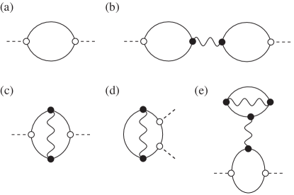
Figure 2: Diagrammatic representation of (a) saddle point contribution and (b-e) the $1/N$ corrections. In our calculation we only include the contribution (b) for reasons explained in the text. The diagram (c) corresponds to a vertex correction relative to (a), while the diagrams (d) and (e) include a Hartree-Fock correction of the single-spinon propagator. The dashed lines represent the external lines, the full lines represent spinon propagators at the SP level and the wavy lines represent the RPA propagator. (Auerbach, 1994)

II.3.1 Saddle Point Approximation

In this approximation the dynamical spin susceptibility is computed by considering the saddle point effective action of Eq. (24) and the single spinon Green’s function of Eq. (28). Each contribution is given by

$$\chi_{{}_{I}\mu\mu}^{\rm sp}(\bm{q},i\omega)=\frac{1}{2}\operatorname{Tr}\left[\mathcal{G}^{\rm sp}u^{\mu}(\bm{q},i\omega)\mathcal{G}^{\rm sp}u^{\mu}(-\bm{q},-i\omega)\right],$$ (65)

and

$$\chi_{{}_{II}\mu\mu}^{\rm sp}(\bm{q},i\omega)\!=\!\frac{1}{4}\operatorname{Tr}\left[\mathcal{G}^{\rm sp}u^{\mu}(\bm{q},i\omega)\right]\operatorname{Tr}\left[\mathcal{G}^{\rm sp}u^{\mu}(-\bm{q},-i\omega)\right].$$ (66)

$\chi_{{}_{II}\mu\mu}^{\rm sp}$ vanishes because $\mathcal{G}^{\rm sp}u^{\mu}$ is traceless for each $\mu$ value. $\chi_{{}_{I}}^{\rm sp}$ is represented diagramatically in Fig. 1 (a) and it coincides with the $\chi^{MF}$ that is obtained from the SBMFT. Mezio et al. (2011)

II.3.2 Gaussian Fluctuations Approximation

To compute Gaussian corrections to $\chi_{\;\mu\mu}^{\rm sp}(\bm{q},i\omega)$, the Green’s function $\mathcal{G}$ that appears in Eqs. (62) and Eq. (63) must be expanded around the saddle point

$$\mathcal{G}\simeq\mathcal{G}^{\rm sp}-\sum_{\alpha}\bigg{[}\mathcal{G}\frac{\partial\mathcal{G}^{-1}}{\partial\phi_{\alpha}}\mathcal{G}\bigg{]}\bigg{|}_{\rm sp}\Delta\phi_{\alpha}.$$ (67)

By replacing Eqs. (67) and (39) in Eq. (62), the Gaussian correction $\chi^{\rm fl}_{I}$ to the dynamical spin susceptibility results

$$\chi_{{}_{I}\mu\nu}^{\rm fl}(\bm{q},i\omega) = \sum_{\alpha_{1}\alpha_{2}}\Bigg{[}\frac{1}{2\mathcal{Z}^{(2)}}\int D[\bar{\phi},\phi]\ \Delta\overline{\phi}_{\alpha_{1}}\Delta\phi_{\alpha_{2}}\ e^{-\sum\limits_{\alpha\alpha^{\prime}}\bar{\phi}_{\alpha}S_{\alpha\alpha^{\prime}}^{(2)}\phi_{\alpha^{\prime}}}\Bigg{]}\times$$ (68)

$$\times \Big{\{}Tr\big{[}\mathcal{G}^{\rm sp}v_{\phi_{\alpha_{1}}}\ \mathcal{G}^{\rm sp}v_{\phi_{\alpha_{2}}}\mathcal{G}^{\rm sp}u^{\nu}(-\bm{q},-i\omega)\mathcal{G}^{\rm sp}u^{\mu}(\bm{q},i\omega)\big{]}+$$

$$+ Tr\big{[}\mathcal{G}^{\rm sp}v_{\phi_{\alpha_{1}}}\ \mathcal{G}^{\rm sp}v_{\phi_{\alpha_{2}}}\mathcal{G}^{\rm sp}u^{\mu}(\bm{q},i\omega)\mathcal{G}^{\rm sp}u^{\nu}(-\bm{q},-i\omega)\big{]}+$$

$$+ \operatorname{Tr}\big{[}\mathcal{G}^{\rm sp}v_{\phi_{\alpha_{1}}}\ \mathcal{G}^{\rm sp}u^{\mu}(\bm{q},i\omega)\mathcal{G}^{\rm sp}v_{\phi_{\alpha_{2}}}\mathcal{G}^{\rm sp}u^{\nu}(-\bm{q},-i\omega)\big{]}\Big{\}}=$$

$$= \sum_{\alpha_{1}\alpha_{2}}D_{\alpha_{2}\alpha_{1}}(\bm{q},i\omega)\big{[}\Gamma_{\alpha_{1}\alpha_{2}\nu\mu}(\bm{q},i\omega)+\Gamma_{\alpha_{1}\alpha_{2}\mu\nu}(\bm{q},i\omega)+\Gamma_{\alpha_{1}\mu\alpha_{2}\nu}(\bm{q},i\omega)\big{]},$$

where

$$D_{\alpha_{2}\alpha_{1}}(\bm{q},i\omega)=\Bigg{[}\frac{1}{\mathcal{Z}^{(2)}}\int D[\bar{\phi},\phi]\ \Delta\overline{\phi}_{\alpha_{1}}\Delta\phi_{\alpha_{2}}\ e^{-\sum\limits_{\alpha\alpha^{\prime}}\bar{\phi}_{\alpha}S_{\alpha\alpha^{\prime}}^{(2)}\phi_{\alpha^{\prime}}}\Bigg{]}=\big{[}(S^{(2)})^{-1}\big{]}_{\alpha_{2}\alpha_{1}}$$ (69)

is the RPA propagator and

$$\Gamma_{\alpha_{1}\alpha_{2}\mu\nu}(\bm{q},i\omega)=\frac{1}{2}\operatorname{Tr}\big{[}\mathcal{G}^{\rm sp}v_{\phi_{\alpha_{1}}}\ \mathcal{G}^{\rm sp}v_{\phi_{\alpha_{2}}}\mathcal{G}^{\rm sp}u^{\mu}(\bm{q},i\omega)\mathcal{G}^{\rm sp}u^{\nu}(-\bm{q},-i\omega)\big{]}.$$ (70)

Replacing Eqs. (67) and (39) in Eq. (63), we obtain the Gaussian correction to the dynamical spin susceptibility

$$\chi_{{}_{II}\;\mu\nu}^{\rm fl}(\bm{q},i\omega) = \sum_{\alpha_{1}\alpha_{2}}\frac{1}{2}\operatorname{Tr}\big{[}\mathcal{G}^{\rm sp}\ v_{\phi_{\alpha_{1}}}\ \mathcal{G}^{\rm sp}\ u^{\mu}(\bm{q},i\omega)\big{]}\times\Bigg{[}\frac{1}{\mathcal{Z}^{(2)}}\int D[\bar{\phi},D\phi]\ \Delta\overline{\phi}_{\alpha_{1}}\Delta\phi_{\alpha_{2}}\ e^{-\sum\limits_{\alpha\alpha^{\prime}}\bar{\phi}_{\alpha}S_{\alpha\alpha^{\prime}}^{(2)}\phi_{\alpha^{\prime}}}\Bigg{]}\times$$ (71)

$$\frac{1}{2}\operatorname{Tr}\big{[}\mathcal{G}^{\rm sp}\ v_{\phi_{\alpha_{2}}}\ \mathcal{G}^{\rm sp}\ u^{\nu}(-\bm{q},-i\omega)\big{]}=\sum_{\alpha_{1}\alpha_{2}}\Lambda_{\mu\alpha_{1}}(\bm{q},i\omega)\ D_{\alpha_{2}\alpha_{1}}(\bm{q},i\omega)\ \Lambda_{\nu\alpha_{2}}(-\bm{q},-i\omega)\ ,$$

where

$$\Lambda_{\mu\alpha}(\bm{q},i\omega)\!=\!\frac{\partial^{2}S_{\rm eff}}{\partial j^{\mu}\partial\phi_{\alpha}}\!=\!\frac{1}{2}\operatorname{Tr}\big{[}\mathcal{G}^{\rm sp}v_{\phi_{\alpha}}\mathcal{G}^{\rm sp}u^{\mu}(\bm{q},i\omega)\big{]}.$$ (72)

The term $\chi_{{}_{II}}^{\rm fl}$ (71) is diagramatically represented in Fig. 2 (b), while Fig. 2 (c) and (d) are the diagrams corresponding to the terms $\chi_{{}_{I}}^{\rm fl}$ (68). In the context of a large-$N$ expansion, these Gaussian corrections to the dynamical susceptibility correspond to $1/N$ contributions. Auerbach and Arovas (1988) However, it can be shown Shindou et al. (2013) that the full Gaussian corrections do not collect all the $1/N$ terms, because the diagram shown in Fig. 2 (e), arising from $S_{int}$ in Eq. (21), is also of order $1/N$. This diagram must then be added to $\chi_{{}_{I}}^{\rm fl}$ of Eq. (68) in order to produce the full $1/N$ correction to the dynamical spin susceptibility.

In the following, we will only include the $1/N$ correction $\chi_{{}_{II}}^{\rm fl}$. There are two reasons for only including this contribution in a first approach to the problem. At the SP level, the local constraint of the SBs is relaxed to a global one, allowing for unphysical bosonic density fluctations (states that are outside the physical Hilbert space). In other words, the density (charge) susceptibility, $\chi^{\rm sp}_{\rm ch}$, which should be zero due to the local constraint (3), becomes finite at the SP level. Arovas and Auerbach demonstrated Arovas and Auerbach (1988) that the inclusion of the diagram shown in Fig. 2 (b) cancels exactly the finite SP charge susceptibility, i.e., $\chi_{\rm ch}=\chi^{\rm sp}_{\rm ch}+\chi^{\rm fl}_{\rm ch}=0$. On the other hand, the inclusion of diagrams (c) and (d) of Fig. 2 requires extra counter terms to fulfil $\chi_{\rm ch}=0$. Auerbach (1994) The second reason for restricting to the diagram shown in Fig. 2 (b) is that it is the only one that can introduce poles (collective modes) in the corrected dynamical susceptibility. Note that the poles of this diagram coincide with the poles of the RPA propagator because both $\chi_{{}_{II}}^{\rm fl}$ and $D_{\alpha_{1},\alpha_{2}}$ are evaluated at the same ${\bm{q}}$ and $\omega$.

Another important observation is that the diagram shown in Fig. 2 (b) vanishes for a singlet ground state ($h=0$). The simple reason is that $\Lambda_{\mu}$ of Eq. (72) can be interpreted as a crossed susceptibility for two fields that belong to different representations of the symmetry group, SU(2), of ${\cal H}$ ( $j^{\mu}$ are components of a vector field, while the auxiliary fields $\phi_{\alpha}$ are scalars). Consequently, $\Lambda_{\mu}$ vanishes for a singlet ground state, leading to the cancellation of $\chi_{{}_{II}}^{\rm fl}$. This result was found by Arovas and Auerbach thirty years ago Arovas and Auerbach (1988) and it is most likely the reason why further attempts of computing $1/N$ corrections to $\chi$ are not found in the subsequent literature. A key observation of this manuscript is that the diagram shown in Fig. 2 (b) does not vanish for the broken symmetry (magnetically ordered) ground state.

Some remarks are in order regarding the zero gauge modes and the computation of $\chi_{{}_{II}}^{\rm fl}$ through Eq. (71). In principle, the computation of the two Gaussian integrals involved in the RPA propagator (69) requires the use of the Faddeev-Popov prescription. However, this prescription can be circumvented due to the orthogonality between $\Lambda_{\mu}$ and the zero gauge modes. This orthogonality arises from the gauge invariance of the effective action, which implies $\frac{\partial S_{\rm eff}}{\partial\theta}=0$ (also $\frac{\partial S_{\rm eff}}{\partial\overline{\theta}}=0$) or

$$\sum_{\alpha}\frac{\partial S_{\rm eff}}{\partial\phi_{\alpha}}\frac{\partial\phi_{\alpha}}{\partial\theta}=0.$$ (73)

This equation is valid for any value of the auxiliary fields. By taking the derivative with respect to the external source $j^{\mu}$, we get

$$\sum_{\alpha}\frac{\partial^{2}S_{\rm eff}}{\partial j^{\mu}\partial\phi_{\alpha}}\frac{\partial\phi_{\alpha}}{\partial\theta}+\frac{\partial S_{\rm eff}}{\partial\phi_{\alpha}}\frac{\partial^{2}\phi_{\alpha}}{\partial j^{\mu}\partial\theta}=0.$$ (74)

The orthogonality between $\Lambda_{\mu\alpha}=\frac{\partial^{2}S_{\rm eff}}{\partial j^{\mu}\partial\phi_{\alpha}}|_{\rm sp}$ and the right zero gauge mode $\vec{\phi}^{R}_{0}$ is obtained after evaluating this equation at the SP values of the auxiliary fields and noticing that the second term vanishes because of the SP condition (20). The same holds for the left zero gauge mode if the effective action is derived with respect to $\overline{\theta}$. If the fluctuations of the auxiliary fields are decomposed into components parallel and perpendicular to the zero gauge mode directions, $\vec{\Delta\phi}=\vec{\phi_{\|}}+\vec{\phi_{\perp}}$, Eq. (71) can be rewritten as follows

$$\chi_{{}_{II}{\mu\nu}}^{\rm fl}(\bm{q},i\omega)=\lim_{\epsilon\rightarrow 0}\frac{\int D[\bar{\phi}_{\|},\phi_{\|}]D[\bar{\phi}_{\perp},\phi_{\perp}]\Lambda_{\mu\alpha_{1}}\times[\overline{\phi}_{\|}+\overline{\phi}_{\perp}]_{\alpha_{1}}[\phi_{\|}+\phi_{\perp}]_{\alpha_{2}}\times\Lambda_{\nu\alpha_{2}}e^{-\epsilon{\bar{\phi}_{\|}}^{\dagger}{\phi_{\|}}-{\bar{\phi}_{\perp}}^{\dagger}S_{\perp}^{(2)}\phi_{\perp}}}{\int D[\bar{\phi}_{\|},\phi_{\|}]D[\bar{\phi}_{\perp},\phi_{\perp}]e^{-\epsilon{\bar{\phi}_{\|}}^{\dagger}{\phi_{\|}}-{\bar{\phi}_{\perp}}^{\dagger}S_{\perp}^{(2)}\phi_{\perp}}},$$ (75)

where the zero modes have been Gaussian regularized by means of the finite positive constant $\epsilon$ in both integrals, which must be sent to zero at the end of the calculation. Negele and Orland (1998) The indices ${\bm{q}}$ and $i\omega$ have been eliminated to make the notation more compact and summation over repeated indices is assumed. The orthogonality between $\Lambda_{\mu}$ and $\phi_{\|}$ implies that Eq. (75) can be factorized as

$$\chi_{{}_{II}\mu\nu}^{\rm fl}(\bm{q},i\omega)=\frac{\int D[\bar{\phi}_{\perp},\phi_{\perp}]\Lambda_{\mu\alpha_{1}}\times\overline{\phi}_{\perp{\alpha_{1}}}\phi_{\perp\alpha_{2}}\times\Lambda_{\nu\alpha_{2}}e^{-{\bar{\phi}_{\perp}}^{\dagger}S_{\perp}^{(2)}\phi_{\perp}}}{\int D[\bar{\phi}_{\perp},\phi_{\perp}]e^{-{\bar{\phi}_{\perp}}^{\dagger}S_{\perp}^{(2)}\phi_{\perp}}}\lim_{\epsilon\rightarrow 0}\frac{\int D[\bar{\phi}_{\|},\phi_{\|}]e^{-\epsilon{\bar{\phi}_{\|}}^{\dagger}{\phi_{\|}}}}{\int D[\bar{\phi}_{\|},\phi_{\|}]e^{-\epsilon{\bar{\phi}_{\|}}^{\dagger}{\phi_{\|}}}}.$$ (76)

Therefore, $\chi^{\rm fl}_{{}_{II}}$ of Eq. (71) can be computed with the matrix $S^{(2)}_{\perp}$ which is the projection of the fluctuation matrix $S^{(2)}$ onto the subspace perpendicular to the zero gauge modes. The same result is obtained if, instead of the Gaussian regularization, we consider a positive zero eigenvalue $\lambda_{0}$ and at the end of the calculation we take the limit $\lambda_{0}\to 0$, in the line of Appendix B. This procedure avoids the use of the Faddeev-Popov prescription. We can conclude that the zero gauge modes do not contribute to the dynamical spin susceptibility because they do not couple to the external magnetic field $j^{\mu}$ contained in $\Lambda_{\mu}$. Shindou et al. (2013)

II.4 Summary of the calculation of Gaussian fluctuations

Here we outline a summary of the main steps followed for the computation of the Gaussian corrections to the different quantities considered in this manuscript:

i) Starting from the partition function (11), the effective action is expanded around its saddle point (21) up to quadratic order (39).

ii) The saddle point approximation leads to a set of self-consistent equations (II.1.1) for the seven parameters $A_{\delta}$, $B_{\delta}$ $\lambda$ (${\delta}>0$ takes three possible values in the triangular lattice). These equations correspond to the SP condition (20) after considering the ansatz  (23).

iii) The seven mean field parameters of the SP solution are plugged in the fluctuation matrix $S^{(2)}$, which for each $(\bm{k},i\omega)$ is a complex non-Hermitian matrix of dimension $13\times 13$ [remember that $\vec{\phi}^{\dagger}\!\!\!=\!\!\!(\overline{W}^{A\;\omega}_{{\bm{k}}\;\delta},{W}^{A\;-\omega}_{{-\bm{k}}\;\delta},\overline{W}^{B\;\omega}_{{\bm{k}}\;\delta},{W}^{B\;-\omega}_{{-\bm{k}}\;\delta},\lambda^{-\omega}_{{-\bm{k}}})$]. The Gaussian fluctuation approximation is stable if all the eigenvalues of the fluctuation matrix have a positive real part (positive-stable condition).

iv) Confirming the presence of the zero gauge modes of the fluctuation matrix is an important sanity check for the correct computation of the fluctuation matrix $S^{(2)}$. This can be done by multiplying the fluctuation matrix (which is computed numerically) by the analytical expression of the zero gauge mode $\vec{\phi}^{R}$ (50).

v) The Faddeev-Popov prescription is applied after confirming the existence of zero gauge modes to carry on the Gaussian integral over genuine fluctuations of the auxiliary fields. Alternatively, the Faddeev-Popov prescription can be avoided by using the truncated matrix $S^{(2)}_{\rm tr}$.

vi) The ground state energy, $E_{\rm gs}(h)=E^{\rm sp}_{\rm gs}(h)+E^{\rm fl}_{\rm gs}(h)$, is obtained by computing $E^{\rm sp}_{\rm gs}(h)$ and $E^{\rm fl}_{\rm gs}(h)$ of Eqs. (II.2) and  (58), respectively.

vii) The local magnetization, $m(h)=m^{\rm sp}_{\rm gs}(h)+m^{\rm fl}(h)$, is obtained by taking the numerical derivative of $E_{\rm gs}(h)$ with respect to $h$.

viii) The dynamical structure factor is obtained via $\mathcal{S}(\bm{q},\omega)=-\frac{1}{\pi}{\rm Im}\chi(\bm{q},\omega)$, after analytic continuation $i\omega\to\omega+i\eta^{+}$ of the dynamical susceptibility $\chi(\bm{q},i\omega)=\chi_{{}_{I}\;\mu\mu}^{\rm sp}(\bm{q},i\omega)+\chi_{{}_{II}\;\mu\mu}^{\rm fl}(\bm{q},i\omega)$, where Eqs. (65) and (71) are used, respectively. It is worth emphasizing that there is no need to perform the Faddeev-Popov trick in this case because the zero gauge modes do not couple to the external sources.

III Spontaneous SU(2) Symmetry Breaking

In this section we investigate the consequences of the spontaneous $SU(2)$ symmetry breaking on the dynamical spin susceptibility. The correct description of this phenomenon requires to carry on the thermodynamic limit of Eq. (71) in the right order:

$$\lim_{h\rightarrow 0}\lim_{N_{s}\rightarrow\infty}\!\mathcal{\chi}_{{}_{II}}^{\rm fl}(\bm{k},i\omega;h)=\!\!\lim_{N_{s}\rightarrow\infty}\!\mathcal{\chi}_{{}_{II}}^{\rm fl}(\bm{k},i\omega;h\!\sim\!N_{s}^{-1}).$$ (77)

To trace back the origin of the symmetry breaking contribution, it is instructive to compare the saddle point Green’s functions in the thermodynamic limit with ($h\neq 0$) and without ($h=0$) the symmetry breaking field. In both cases, the spinons (bosons) condense at $T=0$. Correspondingly, the Green’s function in the thermodynamic limit includes contributions from condensed and non-condensed bosons:

$$\mathcal{G}^{\rm sp}(\bm{k},i\omega)=\mathcal{G}^{\rm sp}_{\rm n}(\bm{k},i\omega)+\mathcal{G}^{\rm sp}_{\rm c}(\bm{k},i\omega).$$ (78)

The energy of the non-condensed bosons remains finite in the thermodynamic limit. Thus, the two limits, $h\to 0$ and $N_{s}\to\infty$, commute for $\mathcal{G}^{\rm sp}_{\rm n}(\bm{k},i\omega)$. In contrast, the energy of the condensed bosons is ${\cal O}(N_{s}^{-1})$, as required by the macroscopic occupation number, implying that $\mathcal{G}^{\rm sp}_{\rm c}(\bm{k},i\omega)$ is linear in $N_{s}$. Because of this factor of $N_{s}$, the change of $\mathcal{G}^{\rm sp}_{\rm c}(\bm{k},i\omega)$ induced by the ${\cal O}(1/N_{s})$ symmetry breaking field in Eq. (77) remains finite in the thermodynamic limit. In other words, the symmetry breaking field only modifies $\mathcal{G}^{\rm sp}_{\rm c}(\bm{k},i\omega)$ in the thermodynamic limit.

The Green’s function for the $SU(2)$ symmetric case ($h=0$) is

$$\mathcal{G}^{\rm sp}_{0}(\bm{k},i\omega)\equiv\lim\limits_{N_{s}\rightarrow\infty}\ \lim\limits_{h\rightarrow 0}\mathcal{G}^{\rm sp}(\bm{k},i\omega;h).$$ (79)

The contribution from the condensate is

$$\mathcal{G}^{\rm sp}_{0-\rm c}(\bm{k},i\omega) =\delta_{{\bm{k}},{\bm{0}}}\left(\frac{g_{0}^{-}(\bm{k}=\bm{0})}{i\omega-\varepsilon_{\bm{0}}}+\frac{g_{0}^{+}(\bm{k}=\bm{0})}{i\omega+\varepsilon_{\bm{0}}}\right)$$ (80)

$$\;\;+\delta_{{\bm{k}},{\bm{Q}}}\left(\frac{g_{0}^{-}(\bm{k}=\bm{Q})}{i\omega-\varepsilon_{\bm{Q}}}+\frac{g_{0}^{+}(\bm{k}=\bm{Q})}{i\omega+\varepsilon_{\bm{Q}}}\right)$$

$$\!+\delta_{{\bm{k}},{\bar{\bm{Q}}}}\left(\frac{g_{0}^{-}(\bm{k}=\bar{\bm{Q}})}{i\omega-\varepsilon_{\bm{\bar{}}{\bm{Q}}}}+\frac{g_{0}^{+}(\bm{k}=\bar{\bm{Q}})}{i\omega+\varepsilon_{\bar{\bm{Q}}}}\right)\ ,$$

with, ${\bm{Q}}$, $\bar{\bm{Q}}\equiv-{\bm{Q}}$ and ${\bm{0}}$ being the condensation wave vectors, and

$$g_{0}^{-}(\bm{k}=\bm{0})=-\left(\begin{array}[]{cccc}v_{\bm{0}}^{{}_{2}}&z_{\bm{0}}&0&0\\ z_{\bm{0}}&u_{\bm{0}}^{{}_{2}}&0&0\\ 0&0&v_{\bm{0}}^{{}_{2}}&z_{\bm{0}}\\ 0&0&z_{\bm{0}}&u_{\bm{0}}^{{}_{2}}\\ \end{array}\right),\ g_{0}^{+}(\bm{k}=\bm{0})=\left(\begin{array}[]{cccc}u_{\bm{0}}^{{}_{2}}&z_{\bm{0}}&0&0\\ z_{\bm{0}}&v_{\bm{0}}^{{}_{2}}&0&0\\ 0&0&u_{\bm{0}}^{{}_{2}}&z_{\bm{0}}\\ 0&0&z_{\bm{0}}&v_{\bm{0}}^{{}_{2}}\\ \end{array}\right),$$ (81)

$$g_{0}^{-}(\bm{k}=\bm{Q})=-\left(\begin{array}[]{cccc}0&0&0&0\\ 0&0&0&0\\ 0&0&v_{\bar{\bm{Q}}-}^{2}&z_{\bar{\bm{Q}}-}\\ 0&0&z_{\bar{\bm{Q}}-}&u_{\bar{\bm{Q}}-}^{2}\\ \end{array}\right),\ g_{0}^{+}(\bm{k}=\bm{Q})=\left(\begin{array}[]{cccc}0&0&0&0\\ 0&0&0&0\\ 0&0&u_{\bar{\bm{Q}}-}^{2}&z_{\bar{\bm{Q}}-}\\ 0&0&z_{\bar{\bm{Q}}-}&v_{\bar{\bm{Q}}-}^{2}\\ \end{array}\right),$$ (82)

$$g_{0}^{-}(\bm{k}=\bar{\bm{Q}})=-\left(\begin{array}[]{cccc}v_{\bar{\bm{Q}}-}^{2}&z_{\bar{\bm{Q}}-}&0&0\\ z_{\bar{\bm{Q}}-}&u_{\bar{\bm{Q}}-}^{2}&0&0\\ 0&0&0&0\\ 0&0&0&0\\ \end{array}\right)\ ,\ g_{0}^{+}(\bm{k}=\bar{\bm{Q}})=\left(\begin{array}[]{cccc}u_{\bar{\bm{Q}}-}^{2}&z_{\bar{\bm{Q}}-}&0&0\\ z_{\bar{\bm{Q}}-}&v_{\bar{\bm{Q}}-}^{2}&0&0\\ 0&0&0&0\\ 0&0&0&0\\ \end{array}\right)\ ,$$ (83)

with $v_{\bm{0}}^{2}=\lim\limits_{h\rightarrow 0}\ v_{\bm{0}\pm}^{2}$, $u_{\bm{0}}^{2}=\lim\limits_{h\rightarrow 0}\ u_{\bm{0}\pm}^{2}$, $z_{\bm{0}}=\lim\limits_{h\rightarrow 0}\ z_{\bm{0}\pm}$, $\varepsilon_{\bm{0}}=\lim\limits_{h\rightarrow 0}\ \varepsilon_{\bm{0}\pm}\sim N_{s}^{-1}$, and $\varepsilon_{\pm\bm{Q}}=\lim\limits_{h\rightarrow 0}\varepsilon_{\pm\bm{Q}-}\sim N_{s}^{-1}$.

Only the ${\bm{k}}={\bm{0}}$ point of the lower band condenses for finite external field $h$ because $\varepsilon_{\bm{0}-}\sim\frac{1}{N_{s}}$. It can be seen that the condensation does not occur at the ${\bm{k}}={\bm{0}}$ point of the higher band and at the $\pm{\bm{Q}}$ points because $\varepsilon_{\bm{0}+},\varepsilon_{\pm\bm{Q}-}\!\sim\!\frac{1}{\sqrt{N_{s}}}$, which does not produce macroscopic occupation number in the thermodynamic limit. The condensate contribution to the Green’s function in the symmetry breaking ($h\neq 0$) case is then modified relative to the $h=0$ case:

$$\mathcal{G}^{\rm sp}_{\rm sb-c}({\bm{k}},i\omega)=\delta_{{\bm{k}},{\bm{0}}}\left(\frac{g_{\rm sb}^{-}({\bm{k}}={\bm{0}})}{i\omega-\varepsilon_{\bm{0}-}}+\frac{g_{\rm sb}^{+}({\bm{k}}={\bm{0}})}{i\omega+\varepsilon_{\bm{0}-}}\right),$$ (84)

with

$$g_{\rm sb}^{-}({\bm{k}}={\bm{0}})=-\frac{1}{2}\left(\begin{array}[]{cccc}v_{\bm{0}-}^{2}&z_{\bm{0}-}&v_{\bm{0}-}^{2}&z_{\bm{0}-}\\ z_{\bm{0}-}&u_{\bm{0}-}^{2}&z_{\bm{0}-}&u_{\bm{0}-}^{2}\\ v_{\bm{0}-}^{2}&z_{\bm{0}-}&v_{\bm{0}-}^{2}&z_{\bm{0}-}\\ z_{\bm{0}-}&u_{\bm{0}-}^{2}&z_{\bm{0}-}&u_{\bm{0}-}^{2}\\ \end{array}\right),\;\;\;\;\;g_{\rm sb}^{+}({\bm{k}}={\bm{0}})=\frac{1}{2}\left(\begin{array}[]{cccc}u_{\bm{0}-}^{2}&z_{\bm{0}-}&u_{\bm{0}-}^{2}&z_{\bm{0}-}\\ z_{\bm{0}-}&v_{\bm{0}-}^{2}&z_{\bm{0}-}&v_{\bm{0}-}^{2}\\ u_{\bm{0}-}^{2}&z_{\bm{0}-}&u_{\bm{0}-}^{2}&z_{\bm{0}-}\\ z_{\bm{0}-}&v_{\bm{0}-}^{2}&z_{\bm{0}-}&v_{\bm{0}-}^{2}\\ \end{array}\right)\ .$$ (85)

By taking the thermodynamic limit of $\Lambda_{\mu\phi}(\bm{q},i\omega)$ [see Eq. (72)] in the presence of symmetry breaking field $h$, we obtain

$$\Lambda_{\mu\phi}(\bm{q},i\omega) = \frac{1}{2}\operatorname{Tr}\left[\ \mathcal{G}^{\rm sp}_{\rm n}\ v_{\phi}\ \mathcal{G}^{\rm sp}_{\rm n}\ u^{\mu}(\bm{q},i\omega)\right]$$

$$+ \frac{1}{2}\operatorname{Tr}\left[\mathcal{G}_{\rm n}^{\rm sp}\ v_{\phi}\ \mathcal{G}_{\rm sb-c}^{\rm sp}\ u^{\mu}(\bm{q},i\omega)\right]$$

$$+ \frac{1}{2}\operatorname{Tr}\left[\mathcal{G}_{\rm sb-c}^{\rm sp}\ v_{\phi}\ \mathcal{G}_{\rm n}^{\rm sp}\ u^{\mu}(\bm{q},i\omega)\right]$$

$$+ \frac{1}{2}\operatorname{Tr}\left[\mathcal{G}_{\rm sb-c}^{\rm sp}\ v_{\phi}\ \mathcal{G}_{\rm sb-c}^{\rm sp}\ u^{\mu}(\bm{q},i\omega)\right]\delta_{\bm{q,0}}\ .$$

The first line vanishes because the non-condensed part of the Green’s function preserves the $SU(2)$ symmetry.  The remaining lines give non-zero contributions because $\mathcal{G}_{\rm sb-c}^{\rm sp}$ is not invariant under the $SU(2)$ symmetry group.

For the polarization matrix $\Pi_{\phi_{\alpha_{1}}\phi_{\alpha_{2}}}$, we have

$$\Pi_{\phi_{\alpha_{1}}\phi_{\alpha_{2}}}\!\!\!\! = \!\!\frac{1}{4}\operatorname{Tr}\left[\mathcal{G}^{\rm sp}_{\rm n}\;v_{\phi_{\alpha_{1}}}\!\mathcal{G}^{\rm sp}_{\rm n}\ v_{\phi_{\alpha_{2}}}\right]$$

$$+ \!\!\frac{1}{4}\operatorname{Tr}\left[\mathcal{G}^{\rm sp}_{\rm n}\ v_{\phi_{\alpha_{1}}}\mathcal{G}_{\rm sb-c}^{\rm sp}\ v_{\phi_{\alpha_{2}}}\right]$$

$$+ \!\!\frac{1}{4}\operatorname{Tr}\left[\mathcal{G}_{\rm sb-c}^{\rm sp}\ v_{\phi_{\alpha_{1}}}\ \mathcal{G}^{\rm sp}_{\rm n}\ v_{\phi_{\alpha_{2}}}\right]$$

$$+ \!\!\frac{1}{4}\operatorname{Tr}\left[\mathcal{G}_{\rm sb-c}^{\rm sp}\ v_{\phi_{\alpha_{1}}}\ \mathcal{G}_{\rm sb-c}^{\rm sp}\ v_{\phi_{\alpha_{2}}}\right]\delta_{\bm{q,0}}\ .$$

In this case all the lines are non-zero because $\Pi_{\phi_{\alpha_{1}}\phi_{\alpha_{2}}}$ is a scalar under spin rotations.

IV Results

This Section includes the results of the formalism presented in Sec. II for the TLHM. The calculations are carried on finite size triangular lattices with $N_{s}=l^{2}+m^{2}+n^{2}$ sites ($l,m,n$ are integer numbers), that have the same discrete symmetries of the infinite triangular lattice, imposing periodic boundary conditions. We have used cluster sizes up to $N_{s}=43200$ and $\eta^{+}=0.01$ for the analytic continuation.

In the following, we present the results of the local magnetization and the dynamical structure factor, and we analyze the long-wavelength limit of the SB theory.

IV.1 Local magnetization

Fig. 3 shows the local magnetization $m(h)=m^{\rm sp}(h)+m^{\rm fl}(h)$ of the $120^{\circ}$ ordering as a function of the symmetry breaking field $h$ for several lattice sizes. These curves are obtained by taking the numerical derivative with respect to $h$ of the ground state energy computed at the Gaussian level, $E_{\rm gs}(h)=E^{\rm sp}_{\rm gs}(h)+E^{\rm fl}_{\rm gs}(h)$, [see Eqs. (II.2) and (58)]. The full circles indicate the magnetization value corresponding to $h=1/N_{s}$. In the inset, these points are extrapolated to the thermodynamic limit along with the SP results (full squares, not shown in the main figure). For the SP extrapolation we can access very large cluster sizes, while for the Gaussian fluctuation approximation we are able to go up to $N_{s}=432$ because of the inacurracies inherent to the numerical derivation. However, it is worth mentioning that the Gaussian correction to the ground state energy can be computed in a reliable way for very large system sizes. Manuel et al. (1998)

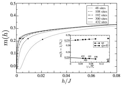
Figure 3: $1/N$ correction of the local magnetization $m$ as a function of the symmetry breaking field $h$ for several lattice sizes. Full circles correspond to $h=1/N_{s}$. Inset: extrapolation to thermodynamic limit of the magnetization for the SP approximation (full squares) and the SP plus Gaussian fluctuations correction (full circles), using $h=1/N_{s}$.

Notably, the Gaussian corrections reduce the SP magnetization from $m^{\rm sp}=0.274$ to $m=0.224$. The latter agrees quite well with the value $m=0.205\pm 0.005$ obtained with the most sophisticated methods like QMC Capriotti et al. (1999) and DMRG. White and Chernyshev (2007) Then, at the Gaussian level, the SB theory seems to support the hypothesis of proximity of the $120^{\circ}$ Néel order to a QMP. For small system sizes (48 and 108 lattices) and $h$ much smaller than the finite size spinon gap, $1/N_{s}$, there is a small region where $m$ has a negative dip. This is a finite size effect that disappears upon increasing $N_{s}$.

IV.2 Dynamical structure factor

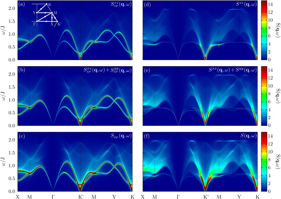
Figure 4: (Color online) First column: dynamical structure factor obtained at the saddle point level: (a) $S_{\rm sp}^{zz}(q,\omega)$, (b) $S_{\rm sp}^{xx}(q,\omega)=S^{yy}_{\rm sp}(q,\omega)$ and (c) $S_{\rm sp}(q,\omega)=S_{\rm sp}^{xx}(q,\omega)+S_{\rm sp}^{yy}(q,\omega)+S_{\rm sp}^{zz}(q,\omega)$. Second column: dynamical structure factor obtained after including the $1/N$ correction (Gaussian fluctuations): (d) $S^{zz}(q,\omega)$, (e) $S^{xx}(q,\omega)=S^{yy}(q,\omega)$ and (f) $S(q,\omega)=S^{xx}(q,\omega)+S^{yy}(q,\omega)+S^{zz}(q,\omega)$. White dashed lines indicate the magnons branches. The path within the hexagonal Brillouin zone is indicated in the inset of panel (a). The results correspond to the triangular lattice size of $N_{s}=120\times 120\times 3=43200$, a value of the magnetic field $h=1/N_{s}$, and analytic continuation $i\omega\rightarrow\omega+i\eta^{+}$ with $\eta^{+}=0.01$.

Fig. 4 shows a comparison between the $S({\bm{q}},\omega)$ obtained at the SP level [see Eq. (65)] and after including the $1/N$ Gaussian correction shown in Fig. 2(b) [see Eq. (71)]. Figs. 4(a-c) clearly show that by properly accounting for the spontaneous symmetry breaking, we obtain different responses for the out of plane, $S^{zz}({\bm{q}},\omega)$, and in-plane, $S^{xx}({\bm{q}},\omega)=S^{yy}({\bm{q}},\omega)$, components of the magnetic structure factor. This natural response of a magnetically ordered ground state should be contrasted with the isotropic one that is obtained with the singlet ground state. Mezio et al. (2011, 2012) As we have already mentioned, the SP solution exhibits a branch of spurious modes arising from density fluctuations that violate the bosonic number constraint (3). However, the main weakness of the SP solution is the lack of magnon modes expected for a magnetically ordered state. The spectrum consists only of a two-spinon continuum (branch cut) because the excitations of the single-spinon condensate are non-interacting spinon modes. Chubukov and Starykh (1995)

The $1/N$ contribution modifies $S({\bm{q}},\omega)$ in a dramatic way [see Figs. 4(d-f)]. The auxiliary gauge field fluctuations bind the spinons into magnons (collective modes) that appear as isolated poles below the two-spinon continuum (TSC). Chubukov and Starykh (1995, 1996) In addition, the cancellation of the density fluctuations Auerbach (1994) produced by the diagram depicted in Fig. 2(b) removes the spurious modes of the SP solution. This cancellation does not persist if we include the other $1/N$ corrections shown in Fig. 2(c-e). The effects of the $1/N$ correction can be better appreciated in the frequency dependence of $S^{zz}({\bm{q}},\omega)$ for a fixed value of momentum ${\bm{k}}=(1.139,0.337)\pi$ between ${\bm{K}}^{\prime}$ and ${\bm{M}}$ (see Fig. 5). The main contributions of the SP solution are cancelled exactly by the $1/N$ correction. This cancellation is accompanied by the emergence of simple poles associated with the collective modes of the ordered state. A similar behavior (not shown in Fig. 5) is obtained for the $S^{xx}({\bm{q}},\omega)$ and $S^{yy}({\bm{q}},\omega)$ components. The removal of the spurious modes and the emergence of magnon poles are the most important qualitative changes relative to the SP solution.

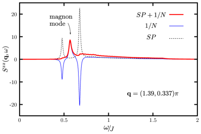
Figure 5: (Color online) Intensity of $S^{zz}({\bm{q}},\omega)$ as a function of the energy $\omega/J$ for ${\bm{k}}=(1.139,0.337)\pi$ (between $K^{\prime}$ and $M$). The dashed (black) and thin (blue) lines correspond to saddle point and $1/N$ correction, separetly. The thick (red) line corresponds to SP plus 1/N correction (Gaussian fluctuations).

Closer inspection of the bottom and the top of the TSC in Figs. 4(d-f) reveals two additional differences. The SP solution exhibits a large spectral weight at the bottom of the TSC, which is transferred to the magnon peak after including the Gaussian correction. In addition, a weak but sharp isolated pole also appears right above the top edge of the TSC. This sharp feature is expected to become overdamped upon inclusion of four and higher spinon excitations resulting from higher orders in the $1/N$ expansion.

Fig. 6 shows a comparison of the resulting single-magnon dispersion (white dashed line), coming from the out of plane $S^{zz}(\bm{k},\omega),$ with the one obtained from series expansions Zheng et al. (2006) (white circles). The strong downward renormalization with respect to LSWT predicted by SE is reproduced by the SB theory at the Gaussian level, along with the appearance of rotonic excitations around the $M$ point. In particular, the quantitative agreement becomes very good when the magnon peaks are sharper, i.e., around the momenta ${\bm{K}}$, ${\bm{K}}^{\prime}$ and ${\bm{M}}$. Consistently with the fact that the ground state of the TLHM is proximate to a quantum melting point, this result supports our original hypothesis of describing the spin-$1$ magnon excitation as a two-spinon bound state.

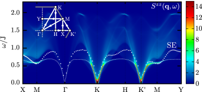
Figure 6: (Color online) Comparison of $S^{zz}({\bm{q}},\omega)$ obtained after including the 1/N correction (Gaussian fluctuations) with the magnon dispersion relation predicted by series expansions Zheng et al. (2006)(SE) (white circles). The dashed line represents the dispersion of the magnon poles.

On the other hand, it is also important to analyze the qualitative differences between Figs. 4(d-f) and the $S({\bm{q}},\omega)$ obtained from a large $S$ expansion. Mourigal et al. (2013) The first obvious qualitative difference is the structure of the high-energy continuum. In semi-classical approaches, this continuum arises from two or more magnon modes. In large-$N$ expansions, it is dominated by two-spinon modes. Consequently, it extends over a wider energy range that is three times bigger than the single magnon bandwith for the case under consideration [see Figs. 4(d-f)].

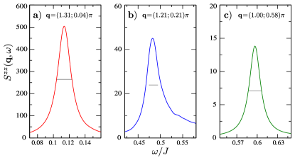
Figure 7: (Color online) Magnon quasi-particle peak for wave vectors (a) ${\bm{q}}=(1.31,0.04)\pi$ and (b) ${\bm{q}}=(1.21,0.21)\pi$ near the ordering wave-vector ${\bf K^{\prime}}$. (c) Single magnon peak at the ${\bf M}$ point. These wave vectors are indicated in Fig. 4(d) with vertical dashed white lines. The segments (thin black line) display the value $2\eta^{+}$ used for the analytic continuation. In all cases $\eta^{+}=0.01$.

Another qualitative difference with large-$S$ expansions is the origin of the magnon quasi-particle peak broadening. As we discuss in the next subsection, the magnon branch gets inside the two-spinon continuum in the long wavelength limit. The kinematic conditions then allow for single-magnon to two spinon decay that broadens the magnon peak. not Upon moving away from the long wavelength limit (region around the $\Gamma$ and the $K$ points) the single-magnon branch is shifted below the two-spinon continuum [see Fig. 4(d-f)] and the intrinsic broadening disappears. A simple phase space argument shows that the broadening of the magnon peak must also go to zero in the $q\to 0$ limit, around $\Gamma$ and $\pm K$ points. Consequently, the strongest effects of the single-magnon to two-spinon decay are expected to occur near the momentum space region where the single-magnon branch is about to emerge from the two spinon continuum. These effects can be observed in Figs. 7(a-c) which display the magnon peak for three representative wave vectors. The wave vector ${\bm{q}}=(1.31,0.04)\pi$ in Fig. 7(a) is very close to the $K$ point. This explains the small broadening that is obtained for this particular wave-vector. As expected from the above-mentioned argument, the magnon peak acquires a much broader structure for ${\bm{q}}=(1.21,0.21)\pi$ [see Fig. 7(b)]. As shown in Fig. 4(f), the magnon peak is emerging from the two-spinon continuum at this particular wave vector. Finally, the broadening of the magnon peak disappears at the ${\bm{M}}$ point [see Fig. 7(c)] because the kinematic conditions no longer allow for single-magnon to two spinon decay (the magnon mode is below the edge of the two-spinon continuum).

Furthermore, it is well known Auerbach and Arovas (1988) that the SP solution violates the sum rule $\int d\omega\sum_{\bm{q}}S({\bm{q}},\omega)=NS(S+1)$ by a factor of 1.5 due to the violation of the local constraint of the SBs. We find that this factor reduces to 1.2 upon including the Gaussian correction shown in Fig. 2b.

Finally, by taking the large-$S$ limit, for $N=2$, we have found that the $1/N$ correction recovers the dynamical structure factor predicted by LSW (to be published elsewhere). This result should be contrasted with the failure of the mean field SB theory to recover the semiclassical dispersion for spiral states. Coleman and Chandra (1994); Mattsson (1995)

IV.3 Long Wavelength Limit

Linear spin wave theory is expected to work well in the long wavelength limit. Dombre and Read (1989) Consequently, although the current approach is motivated by the experimental observation of anomalies in the dynamical spin structure factor that appear at wavelengths comparable to the lattice parameter, it is still interesting to analyze the outcome of our approach in the long wavelength limit. In this limit the spectrum consists of the three low-energy Goldstone modes around $\bm{0}$ and $\pm{\bm{Q}}:$ (i) $\rvert\bm{k}\rvert<\Lambda$; (ii) $\rvert\bm{k}-\bm{Q}\rvert<\Lambda$; (iii) $\rvert\bm{k}+\bm{Q}\rvert<\Lambda$, where $\Lambda$ is a momentum cut-off below which the dispersion relation is practically linear. These collective modes (magnons) are obtained as poles of the RPA propagator

$$D(\bm{q},i\omega)=\left[\Pi_{0}-\Pi(\bm{q},i\omega)\right]^{-1},$$ (88)

where the polarization operator, $\Pi(\bm{q},i\omega)$, is determined by the degrees of freedom with wavelength longer than $\Lambda^{-1}$. The effective low-energy action for the spinons and their coupling to the gauge field is obtained by performing a gradient expansion of the effective action (see Appendix D).

IV.3.1 Around the $\Gamma$ point

To obtain results in the long wavelength limit, we must expand the polarization operator in powers of $q$ and $\omega$. According to Eq. (III), the polarization operator can be decomposed into three contributions. The first line of Eq. (III) corresponds to a contribution from the non-condensed bosons only. We will refer to this contribution as ${\Pi}_{nn}$. The second and the third line of Eq. (III) correspond to a mixed contribution from the condensed and non-condensed bosons and will be denoted as ${\Pi}_{cn}$. Finally, the last line of Eq. (III) corresponds to a contribution from the condensed bosons only, that will be denoted as ${\Pi}_{cc}$.

The leading order contribution to $\Pi(\bm{q},i\omega)$ is ${\cal O}(q^{-2})$

$$\Pi_{cn}^{(-2)}(\bm{q},i\omega)=\frac{\phi Z/2}{c^{2}q^{2}+\omega^{2}}\Theta,$$ (89)

where $\phi$ refers to the density of condensed bosons, $Z=\lambda+\gamma_{\bm{Q}/2}^{B}$, and $\Theta=\theta\rvert u_{1}\rangle\langle v_{1}\rvert$ after a singular value decomposition (SVD) (see Appendix D). Given that $\Pi_{cn}^{(-2)}(\bm{q},i\omega)$ diverges for $\rvert\bm{q}\rvert,\omega\rightarrow 0$, it is clear that the magnon mode belongs to the null space ${\cal P}$ of $\Pi_{cn}^{(-2)}(\bm{q},i\omega)$. Therefore, to extract the magnon pole, we just need to consider the next order contributions to the polarization matrix projected into the null subspace ${\cal P}$:

$${\bar{\Pi}}=P_{L}\cdot\Pi\cdot P_{R},$$ (90)

with the left/right projectors

$$P_{L} = \sum_{\sigma>1}\rvert u_{\sigma}\rangle\langle u_{\sigma}\rvert,$$ (91)

$$P_{R} = \sum_{\sigma>1}\rvert v_{\sigma}\rangle\langle v_{\sigma}\rvert,$$ (92)

where $\langle u_{\sigma}\rvert u_{1}\rangle=0$ and $\langle v_{\sigma}\rvert v_{1}\rangle=0$ for $\sigma>1$. It turns out that the projection of the ${\cal O}(q^{-1})$ contributions, that we denote as $\Pi^{(-1)}$, is equal to zero. However, $\Pi^{(-2)}$ still connects the subspace ${\cal P}$ with the orthogonal subspace, leading to a ${\cal O}(1)$ contribution within the subspace ${\cal P}$ that is obtained via a second order process:

$${\bar{\Pi}}^{(0)}_{1}(\bm{q},i\omega)= -P_{L}\cdot\frac{\Pi_{cn}^{(-1)}\rvert v_{1}\rangle\langle u_{1}\rvert\Pi_{cn}^{(-1)}}{\langle u_{1}\rvert\Pi_{cn}^{(-2)}\rvert v_{1}\rangle}\cdot P_{R},$$ (93)

where

$${\bar{\Pi}}_{cn}^{(-1)}(\bm{q},i\omega)={\phi q\over c^{2}q^{2}+\omega^{2}}\left({i\omega\over 2q}{\bar{\Gamma}}+{Z\over 4}\hat{\bm{q}}\cdot{\bar{\bm{M}}}\right).$$ (94)

Here we used the notation ${\bar{A}}\equiv P_{L}\cdot A\cdot P_{R}$ for any matrix $A$. $\bar{\Gamma}$ and $\bar{M}$ are defined in in the Appendix D. The non-condensed bosons give no contribution to this second order process.

In addition to ${\bar{\Pi}}^{(0)}_{1}(\bm{q},i\omega)$, we must consider the other ${\cal O}(1)$ contributions to the polarization operator. The contribution ${\bar{\Pi}}_{nn}^{(0)}(\bm{q},i\omega)$ from the non-condensed bosons is a regular integral that depends on the cutoff $\Lambda$. Finally, the ${\cal O}(1)$ contribution arising from the combination of condensed and non-condensed bosons is

$${\bar{\Pi}_{cn}}^{(0)}(\bm{q},i\omega)\!\!=\!\!\frac{\phi q^{2}/2}{c^{2}q^{2}+\omega^{2}}\left(\bar{\Sigma}\!+\!{i\omega\over q}\hat{\bm{q}}\cdot\bar{{\bm{R}}}+{Z\over 2}\hat{\bm{q}}\cdot\bar{{\bm{D}}}\cdot\hat{\bm{q}}\right),$$ (95)

where these matrices $\Sigma$, $\bm{R}$ and $\bm{D}$ are defined in Appendix D.

We note that $\Pi_{cc}$ is not included in this analysis because it only gives a finite contribution at the condensate wave vector, while we are only interested in the behavior of $\Pi$ around these points ($q$ can be arbitrarily small but always finite)

In summary, the magnon mode in the long wavelength limit is obtained from the solution of the equation:

$$\det\left[\left({\bar{\Pi}}_{0}-{\bar{\Pi}}_{nn}^{(0)}-{\bar{\Pi}}_{cn}^{(0)}-{\bar{\Pi}}^{(0)}_{1}\right)\right]=0.$$ (96)

The left hand side of this equation is a function of $\omega/q$. Thus the root of this function gives $\omega=v_{\Gamma}q$, with magnon velocity $v_{\Gamma}=1.087J$. The fact that $v_{\Gamma}$ turns out to be a real number confirms that the magnon mode is a well-defined quasi-particle in the long wavelength limit. The magnon velocity at the $\Gamma$ point obtained with a $1/S$ expansion up to ${\cal O}(S^{-1})$ is $1.15J$. Chubukov et al. (1994); Chernyshev and Zhitomirsky (2009)

Near the magnon pole, the polarization operator takes the form:

$$\lim_{\rvert\bm{q}\rvert,\omega\rightarrow 0}\Pi(\bm{q},\omega>0)=\alpha\left(1-{\omega\over vq}\right)\rvert\mu_{m}\rangle\langle\nu_{m}\rvert+...,$$ (97)

where $\rvert\mu_{m}\rangle$ and $\rvert\nu_{m}\rangle$ refer to the magnon mode in the null subspace ${\cal P}$ and “…” abbreviates the regular contributions from the orthogonal subspaces. According to our derivation, the leading order correction to Eq. (97) is ${\cal O}(q)$. The pole equation is modified by the matrix element of $\Delta\Pi(\bm{q},\omega)\equiv\Pi(\bm{q},\omega)-\lim_{\rvert\bm{q}\rvert,\omega\rightarrow 0}\Pi(\bm{q},\omega)$ in the subspace of the magnon mode described by the left (or right) state $\rvert\mu_{m}\rangle$ (or $\rvert\nu_{m}\rangle$), namely

$$\alpha\left(1-{i\omega\over vq}\right)=\langle\mu_{m}\rvert\Delta\Pi(\bm{q},\omega)\rvert\nu_{m}\rangle.$$ (98)

The contribution from the condensed bosons is analytic at $\rvert\bm{q}\rvert=0$ for a given ratio of $\omega/q$. Consequently, the leading order contribution to the matrix element $\langle u_{m}\rvert\Delta\Pi_{cn}(\bm{q},\omega)\rvert v_{m}\rangle$ is

$$\langle\mu_{m}\rvert\Delta\Pi_{cn}(\bm{q},\omega)\rvert\nu_{m}\rangle\propto qF\left(\frac{\omega}{cq}\right)\ .$$ (99)

This contribution gives rise to a non-linear correction $\sim q^{2}$ to the magnon dispersion, but no contribution to the magnon decay because of the energy mismatch upon splitting the magnon into a non-condensed (with momentum $\bm{q}$) and a condensed (with $\bm{0}$ momentum) spinon.

The contribution from the non-condensed bosons, $\Pi_{nn}^{\rm reg}(\bm{q},\omega)$, is not guaranteed to be analytic in $\bm{q}$ at $\bm{q}=\bm{0}$ for given ratio of $\omega/q$. Therefore, we assume

$$\langle\mu_{m}\rvert\Delta\Pi_{nn}(\bm{q},\omega)\rvert\nu_{m}\rangle\propto q^{\gamma}H\left(\frac{\omega}{cq}\right).$$ (100)

Because the magnon velocity is higher than the spinon velocity, the kinematic conditions enable the decay of one magnon into two slow spinons. not This process gives rise to an imaginary part of $H({\omega\over cq})$. Consequently, the magnon pole moves away from the real axis leading to a finite decay rate $\Gamma_{q}\propto q^{1+\gamma}$. A numerical solution of the determinant of $\Pi_{0}-\Pi(\bm{q},i\omega)$ gives $\gamma=1$, implying that $\Gamma_{q}\propto q^{2}$.

IV.3.2 Around the $\pm K$ points

The magnon modes around $\pm K$ are connected by inversion symmetry. Thus, without loss of generality, we only consider the magnon dispersion around the $K$ point. The structure of the polarization operator $\Pi(\bm{q}+\bm{Q},i\omega)$ is much simpler than the one obtained for the $\Gamma$ point. The contribution from the non-condensed bosons is regular in the long wavelength limit,

$$\lim_{\bm{q}\rightarrow 0,\omega\rightarrow 0}\Pi_{nn}(\bm{q}+\bm{Q},i\omega)=\Pi_{nn}(\bm{Q},0),$$ (101)

while the contribution from the condensed bosons is

$$\Pi_{cn}(\bm{q}+\bm{Q},i\omega)={\phi q^{2}/2\over c^{2}q^{2}+\omega^{2}}\left(\Sigma^{K}+Z\hat{\bm{q}}\cdot\bm{Q}^{K}\cdot\hat{\bm{q}}\right).$$ (102)

By applying the procedure that we described for the $\Gamma$ point, we obtain a magnon velocity $v_{K}=1.033J$, which is very close to the value $v_{K}=0.9948J$ obtained by non-linear spin wave theory [up to ${\cal O}(S^{-1})$]. Chubukov et al. (1994); Chernyshev and Zhitomirsky (2009) The non-linear correction to the magnon dispersion is ${\cal O}(q^{2})$, while the decay rate $\Gamma_{q}$ turns out to be proportional to $q^{5/2}$.

V Discussion

In summary, we have demonstrated that the Gaussian corrections of the Schwinger boson approach to the TLHAM eliminates serious limitations of the SP approximation and provides much better description of the order parameter and the dynamical response of magnetically ordered states. This description becomes particularly appealing in the proximity of transitions into spin liquids. Here we have focused on the $1/N$ correction introduced by the diagram shown in Fig. 2b. The main reason is that this is the only diagram that generates poles in $S({\bm{q}},\omega)$ at the $1/N$ level. The rest of the $1/N$ diagrams shown in Fig. 2(c-e) renormalizes the interaction vertex, as well as the single-spinon propagator. It is important to note that these diagrams generate four-spinon contributions that will extend the high-energy spectral weight beyond the two-spinon continuum shown in Fig. 4.

The magnon excitations obtained from the $1/N$ correction considered in this manuscript consist in two-spinon bound states. Its dispersion agrees well with the magnon dipersion obtained from series expansions Zheng et al. (2006) in the regions where the magnon spectral weight is high. Moreover, the magnon velocities obtained by taking the long wavelength limit around the ${\Gamma}$ and the ${\pm K}$ points agree very well with the result obtained from linear spin wave theory plus $1/S$ corrections. Chubukov et al. (1994); Chernyshev and Zhitomirsky (2009) At the $1/N$ level, the magnon decay occurs via emission of two-spinons. Given that spinons are not low-energy modes of the Higgs phase (they are gapped out by the Higgs mechanism), this mechanism should be replaced by the more traditional single magnon to two magnon-decay in the long wavelength limit of the theory. However, to capture the single-magnon to two magnon decay within this formalism, it is necessary to include $1/N^{2}$ corrections, such as the diagram shown in Fig. 8. While the inclusion of two-magnon and four spinon processes is beyond the scope of this manuscript, we must keep in mind that these corrections are necessary to reproduce some aspects of $S({\bm{q}},\omega)$, such as the magnon broadening in the long wavelength limit or high energy contributions arising from the four-spinon continuum.

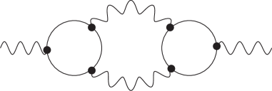
Figure 8: Diagram of order $1/N^{2}$ for the RPA propagator that accounts for the single-magnon to two magnon decay process. Note the similarity between this diagram and the lowest order diagram in a $1/S$ expansion that accounts for the single-magnon to two-magnon decay (each wavy line must be interpreted as a magnon propagator, while each internal loop must be interpreted as a cubic vertex).

Recent inelastic neutron scattering measurements in Ba₂CoSb₂O₉ Ito et al. (2017) have revealed a three-stage energy structure in $S({\bm{q}},\omega)$ composed of single-magnon low-energy excitations and two high-energy dispersive excitation continua whose peaks are separated by an energy scale of order $J$. Based on the results obtained in this manuscript, we speculate that the two stage high-energy structure arises from two-spinon and four-spinon contributions. Testing this conjecture requires not only the inclusion of additional diagrams, but also an extension of the formalism presented in this manuscript to the case of a 3D lattice (vertically staked triangular layers) with anisotropic exchange interaction (Ba₂CoSb₂O₉ has a small easy-plane exchange anisotropy).

Because of the proximity of the $120^{\circ}$ Néel order ground state to a spin liquid state, we have used the $S=1/2$ triangular AFM Heisenberg model as an example of application. However, this formalism can be applied to other magnetically ordered states in the proximity of a spin liquid phase. The current quest for materials that can realize quantum spin liquids calls for approaches that capture the signatures of fractional excitations in the dynamical response. Given that most of these materials exhibit some form of magnetic ordering at low enough temperatures, our approach is addressing the increasing demand of modeling and understanding the dynamical response of quantum magnets in the proximity of a quantum melting point.

Appendix A Complex Gaussian integrals

In order to compute the Gaussian correction to the partition function, we need to derive the necessary condition for the convergence and the value of the complex Gaussian integral

$$Z=\int D[\vec{\phi}^{\dagger},\vec{\phi}]e^{-\vec{\phi}^{\dagger}\cdot\bm{A}\cdot\vec{\phi}},$$ (103)

where $\vec{\phi}=\left(\phi_{1},\cdots,\phi_{n}\right)\in{\mathbb{C}}^{n},$ $\vec{\phi}^{\dagger}$ is the Hermitian conjugate of $\vec{\phi}$, the measure is given by $D[\vec{\phi}^{\dagger},\vec{\phi}]=\prod_{\mu=1}^{n}\frac{d\bar{\phi}_{\mu}d\phi_{\mu}}{2\pi i},$ and $\bm{A}$ is a $n\times n$ complex matrix diagonalizable, not necessarily Hermitian.

As $\bm{A}$ is diagonalizable, there exists a non-singular matrix $\bm{R}$ such that $\bm{A}$ can be transformed into a diagonal matrix $\bm{\Lambda}(\Lambda_{\mu\nu}=\lambda_{\mu}\delta_{\mu\nu})$ through the similarity transformation

$$\bm{A}=\bm{R}\cdot\bm{\Lambda}\cdot\bm{R}^{-1}.$$ (104)

The diagonal entries of $\bm{\Lambda}$ are the (complex) eigenvalues of $\bm{A}$, while the vector columns of $\bm{R}$ are the corresponding right-eigenvectors, $\bm{A}\cdot\vec{\phi}^{R}_{\mu}=\lambda_{\mu}\vec{\phi}^{R}_{\mu}.$ On the other hand, the rows of $\bm{L}\equiv\bm{R}^{-1}$ are the left-eigenvectors of $\bm{A}$, that is $\vec{\phi}^{L}_{\mu}\cdot\bm{A}=\lambda_{\mu}\vec{\phi}^{L}_{\mu}$. Notice that if $\bm{A}$ is non-Hermitian, $\bm{R}$ is not unitary and, as a consequence, the right-eigenvectors are not orthogonal among themselves. The same is valid for the set of left-eigenvectors. However, as $\bm{L}\cdot\bm{R}=\bm{I}$, right-eigenvectors are orthonormalized with respect to the left-eigenvectors.

Using Eq. (104) and performing the linear transformation $\vec{\phi}=\bm{R}\cdot\vec{z},$ , whose Jacobian is given by $\det(\bm{R}^{\dagger}\cdot\bm{R}),$ $Z$ becomes

$$Z=\det{\bm{G}}\int D[\vec{z}^{\dagger},\vec{z}]e^{-\vec{z}^{\dagger}\cdot\bm{G}\cdot\bm{\Lambda}\cdot\vec{z}},$$ (105)

where the measure is $D[\vec{z}^{\dagger},\vec{z}]=\prod_{\mu=1}^{n}\frac{d\bar{z}_{\mu}dz_{\mu}}{2\pi i}$ and we have defined the Gram matrix $\bm{G}\equiv\bm{R}^{\dagger}\cdot\bm{R},$ whose elements are given by the inner product of the right-eigenvectors, $G_{\mu\nu}=\vec{\phi}^{R\dagger}_{\mu}\cdot\vec{\phi}^{R}_{\nu}$. $\bm{G}$ is Hermitian, and positive-definite as the bilinear form

$$\vec{z}^{\dagger}\cdot\bm{G}\cdot\vec{z}=\left|\left|\sum_{\mu}z_{\mu}\vec{\phi}^{R}_{\mu}\right|\right|^{2}>0\;\;{\rm for}\;\;{\bm{z}\neq\bm{0}}.$$

Now, we will prove that, given a $n\times n$ diagonal matrix $\bm{\Lambda}$ whose diagonal entries $\lambda_{\mu}$ all have a positive real part, and a $n\times n$ Hermitian positive-definite matrix $\bm{G}$:

$$I_{n}(\bm{G},\bm{\Lambda})\equiv\int D[\vec{z}^{\dagger},\vec{z}]e^{-\vec{z}^{\dagger}\cdot\bm{G}\cdot\bm{\Lambda}\cdot\vec{z}}=\frac{1}{\det(\bm{G}\cdot\bm{\Lambda})}.$$ (106)

We prove this result by induction. For $n=1$,

$$I_{1}(\bm{G},\bm{\Lambda})=\int\frac{d\bar{z}_{1}dz_{1}}{2\pi i}e^{-G_{11}\lambda_{1}|z_{1}|^{2}}$$

where $\bm{G}$ is the positive real number $G_{11}.$ The analytical continuation of the well-known integral $\int\frac{d\bar{z}dz}{2\pi i}e^{-a|z|^{2}}=\frac{1}{a},$ easily computed for real $a>0,$ shows that $I_{1}$ converges if $\operatorname{\rm Re}\lambda_{1}>0$, and its value is given by

$$I_{1}(\bm{G},\bm{\Lambda})=\frac{1}{G_{11}\lambda_{1}}\equiv\frac{1}{\det(\bm{G}\cdot\bm{\Lambda})}.$$

So, for $n=1$ the integral (106) is valid. Now we calculate the integral for a generic $n$, assuming its validity for $n-1$.

$$I_{n}(\bm{G},\bm{\Lambda}) = \int\prod_{\mu=1}^{n-1}\frac{d\bar{z}_{\mu}dz_{\mu}}{2\pi i}\exp\left[-\sum_{\mu\nu=1}^{n-1}\bar{z}_{\mu}G_{\mu\nu}\lambda_{\nu}z_{\nu}\right]\times$$ (107)

$$\times\int\frac{d\bar{z}_{n}dz_{n}}{2\pi i}\exp\left[-S^{(n)}(\vec{z}^{\dagger},\vec{z})\right],$$

where

$$S^{(n)}(\vec{z}^{\dagger},\vec{z}) = G_{nn}\lambda_{n}|z_{n}|^{2}+$$

$$+\bar{z}_{n}\sum_{\nu=1}^{n-1}G_{n\nu}\lambda_{\nu}z_{\nu}+z_{n}\sum_{\mu=1}^{n-1}G_{\mu n}\lambda_{n}\bar{z}_{\mu}.$$

As $\bm{G}$ is positive-definite, all its diagonal elements are positive real numbers. Hence, the integral over $\bar{z}_{n},z_{n}$ in Eq. (107) is convergent if $\operatorname{\rm Re}\lambda_{n}>0.$ Using the well known integral $\int\frac{d\bar{z}dz}{2\pi i}e^{-a|z|^{2}+J\bar{z}+J^{\prime}z}=\frac{1}{a}\exp[\frac{JJ^{\prime}}{a}],$ valid for $\operatorname{\rm Re}a>0$ and complex $J,J^{\prime}$, the integral is given by

$$\frac{1}{G_{nn}\lambda_{n}}\exp\left[\sum_{\mu\nu=1}^{n-1}\bar{z}_{\mu}\frac{G_{\mu n}G_{n\nu}}{G_{nn}}\lambda_{\nu}z_{\nu}\right].$$ (109)

After performing the integration over $\bar{z}_{n},z_{n}$, $I_{n}$ (107) is given by a $(n-1)$-dimensional complex Gaussian integral

$$I_{n}(\bm{G},\bm{\Lambda})=\frac{1}{G_{nn}\lambda_{n}}I_{n-1}((\bm{G}/G_{nn}),\bm{\tilde{\Lambda}})$$ (110)

where the $(n-1)\times(n-1)$ matrix $(\bm{G}/G_{nn})$ is the so-called Schur complement of $\bm{G}$ with respect to $G_{nn}$, Horn and Johnson (2012) defined as

$$(\bm{G}/G_{nn})_{\mu\nu}=G_{\mu\nu}-\frac{G_{\mu n}G_{n\nu}}{G_{nn}},$$ (111)

while $\bm{\tilde{}}\Lambda$ is the diagonal $(n-1)\times(n-1)$ matrix that results from taking out the $n$-th row and the $n$-th column in $\bm{\Lambda}.$ $(\bm{G}/G_{nn})$ is a Hermitian and positive-definite matrix. To prove this last statement, we take into account that $\bm{G}$ is positive-definite, that is

$$\vec{z}^{\dagger}\cdot\bm{G}\cdot\vec{z} = \sum_{\mu,\nu=1}^{n-1}\bar{z}_{\mu}G_{\mu\nu}z_{\nu}+\bar{z}_{n}\sum_{\nu=1}^{n-1}G_{n\nu}z_{\nu}+$$

$$+ \sum_{\mu=1}^{n-1}\bar{z}_{\mu}G_{\mu n}z_{n}+G_{nn}|z_{n}|^{2}>0,$$

for all non-zero $\vec{z}\in{\mathbb{C}}^{n}$. In particular, if we take $z_{n}=-\frac{1}{G_{nn}}\sum_{\nu=1}^{n-1}G_{n\nu}z_{\nu},$ we get $\vec{z}^{\dagger}\cdot(\bm{G}/G_{nn})\cdot\vec{z}>0,$ for all non-zero $\vec{z}\in{\mathbb{C}}^{n-1}.$ As $(\bm{G}/G_{nn})$ is Hermitian positive-definite, and the real part of all the diagonal entries of $\bm{\tilde{\Lambda}}$ are positive, the $(n-1)$-dimensional complex integral in (110), by hypothesis, equals $1/\det((\bm{G}/G_{nn})\cdot\bm{\tilde{\Lambda}})$, and it results in

$$I_{n}(\bm{G},\bm{\Lambda})=\frac{1}{G_{nn}\det(\bm{G}/G_{nn})}\times\frac{1}{\det\bm{\Lambda}}.$$ (112)

The Schur’s identity Horn and Johnson (2012) tell us that, if $G_{nn}\neq 0$,

$$\det\bm{G}=G_{nn}\det(\bm{G}/G_{nn}).$$ (113)

Replacing the identity in Eq. (112), we end the proof of the Gaussian integral

$$\int D[\vec{z}^{\dagger},\vec{z}]e^{-\vec{z}^{\dagger}\cdot\bm{G}\cdot\bm{\Lambda}\cdot\vec{z}}=\frac{1}{\det(\bm{G}\cdot\bm{\Lambda})}.$$ (114)

The application of above equation to the integral $Z$ as expressed in Eq. (105) allows us, on one hand, to establish the convergence condition of the original Gaussian integral (103). That is, all the eigenvalues of the $\bm{A}$ matrix should have a positive real part. A matrix with this property is called a positive-stable matrix. On the other hand, we get

$$Z=\int D[\vec{\phi}^{\dagger},\vec{\phi}]e^{-\vec{\phi}^{\dagger}\cdot\bm{A}\cdot\vec{\phi}}=\frac{1}{\det\bm{A}},$$ (115)

since $\det\bm{\Lambda}=\det\bm{A}$. This result is the generalization of the usual complex Gaussian integral, where it is requested that $\bm{A}$ or its real part be positive-definite matrices. It can be shown that, while any matrix with a positive-definite real part is a positive-stable matrix, the converse is not true.

An alternative way to arrive at the positive-stable condition for the convergence of the Gaussian integral is to use the analytical continuation of the Gaussian integral with a Hermitian matrix. Kamenev and Levchenko (2009)

Appendix B Faddeev-Popov treatment of zero modes

In this Appendix, we show how to derive the partition function in the presence of zero gauge modes, by means of the Faddeev-Popov prescription.

Let $Z$ be the Gaussian integral

$$Z=\int D[\vec{\phi}^{\dagger},\vec{\phi}]e^{-\vec{\phi}^{\dagger}\cdot\bm{A}\cdot\vec{\phi}}$$ (116)

where $\bm{A}$ is a diagonalizable matrix that has a zero eigenvalue, with its corresponding right $\vec{\phi}^{R}_{0}$ and left $\vec{\phi}^{L}_{0}$ eigenvectors. In our case, this zero mode is the consequence of the invariance of $Z$ under a $U(1)$ gauge transformation characterized by the (complex) phase $\theta$, whose expression is

$$\vec{\phi}\to\vec{\phi}(\theta)=\vec{\phi}+\theta\vec{\phi}^{R}_{0},\;\;\vec{\phi}^{\dagger}\to\vec{\phi}^{\dagger}(\bar{\theta})=\vec{\phi}^{\dagger}+\bar{\theta}\vec{\phi}_{0}^{L}.$$ (117)

In fact, the exponent of the Gaussian integral is gauge invariant, $\vec{\phi}^{\dagger}(\bar{\theta})\cdot\bm{A}\cdot\vec{\phi}(\theta)=\vec{\phi}^{\dagger}\cdot\bm{A}\cdot\vec{\phi}$, and the transformation (117) has a unit Jacobian.

For a positive-stable $\bm{A}$, the Gaussian integral (116) is given by $\det^{-1}({\bm{A}})$ (see Appendix A). As a consequence, the presence of a zero eigenvalue implies its divergence, and this signals the absence of a restoring force along the zero mode direction, due precisely to the gauge symmetry. However, using the Faddeev-Popov trick we can exactly extract from $Z$ the contribution of the gauge group volume $\int\frac{d\bar{\theta}d\theta}{2\pi i}$ –that counts the redundant gauge degree of freedom that give rise to such divergence–, remaining a physically sound result from the integration of the genuine Gaussian fluctuations.

To proceed with the Faddeev-Popov trick, first we define a Dirac delta function on the complex plane by means of the integral representation

$$\delta(\bar{z},z)=\int\frac{d\bar{\alpha}d\alpha}{2\pi i}e^{i(\bar{\alpha}z+\bar{z}\alpha)},$$ (118)

such that $\delta(\bar{z},z)$ satisfies, for a given function $F$, the usual relation

$$\int\frac{d\bar{z}dz}{2\pi i}\delta(\bar{z},z)F(\bar{z},z)=F(0,0).$$ (119)

Indeed,

$$\delta(\bar{z},z)=\int\frac{d\alpha_{R}d\alpha_{I}}{\pi}e^{2i(\alpha_{R}x+\alpha_{I}y)}=\pi\delta(x)\delta(y),$$ (120)

where $\alpha=\alpha_{R}+i\alpha_{I}$ and $z=x+iy$. Replacing (120) in Eq. (119), we get the usual property of the Dirac delta function.

To get rid of the (divergent) gauge fluctuations, we impose natural gauge fixing conditions that constraint the fluctuations to be orthogonal to the zero mode, Trumper et al. (1997)

$$g(\bar{\theta})=\vec{\phi}^{\dagger}(\bar{\theta})\cdot\hat{\phi}^{R}_{0}=0,\;\;h(\theta)=\hat{\phi}^{L}_{0}\cdot\vec{\phi}(\theta)=0,$$ (121)

where we have defined the zero mode “versors” as $\hat{\phi}^{L}_{0}\equiv\vec{\phi}^{L}_{0}/\sqrt{\vec{\phi}^{L}_{0}\cdot\vec{\phi}^{R}_{0}}$ and $\hat{\phi}^{R}_{0}\equiv\vec{\phi}^{R}_{0}/\sqrt{\vec{\phi}^{L}_{0}\cdot\vec{\phi}^{R}_{0}}.$ Taking into account Eq. (117), the gauge fixing conditions are given by

$$g(\bar{\theta}) = \vec{\phi}^{\dagger}\cdot\hat{\phi}^{R}_{0}+\bar{\theta}\sqrt{\vec{\phi}^{L}_{0}\cdot\vec{\phi}^{R}_{0}},$$ (122)

$$h(\theta) = \hat{\phi}^{L}_{0}\cdot\vec{\phi}+\theta\sqrt{\vec{\phi}^{L}_{0}\cdot\vec{\phi}^{R}_{0}},$$

and they are imposed in $Z$ through the Faddeev-Popov trick, that consists in the construction of the unit as

$$1=\Delta_{\rm FP}(\vec{\phi}^{\dagger},\vec{\phi})\times\int\frac{d\bar{\theta}d\theta}{2\pi i}\delta(g(\bar{\theta}),h(\theta)),$$ (123)

where $\Delta_{\rm FP}$ is the so-called Faddeev-Popov determinant. To compute it, we first replace the Dirac delta distribution by its integral representation and express the gauge conditions by means of Eq. (122):

$$\int\frac{d\bar{\theta}d\theta}{2\pi i}\delta(g(\bar{\theta}),h(\theta)) = \int\frac{d\bar{\alpha}d\alpha}{2\pi i}e^{i\left(\bar{\alpha}\vec{\phi}^{\dagger}\cdot\hat{\phi}^{R}_{0}+\alpha\hat{\phi}^{L}_{0}\cdot\vec{\phi}\right)}\int\frac{d\bar{\theta}d\theta}{2\pi i}e^{i\sqrt{\vec{\phi}^{L}_{0}\cdot\vec{\phi}^{R}_{0}}\left(\bar{\theta}\alpha+\theta\bar{\alpha}\right)}=$$

$$= \int\frac{d\bar{\alpha}d\alpha}{2\pi i}e^{i\left(\bar{\alpha}\vec{\phi}^{\dagger}\cdot\hat{\phi}^{R}_{0}+\alpha\hat{\phi}^{L}_{0}\cdot\vec{\phi}\right)}\delta\left(\sqrt{\vec{\phi}^{L}_{0}\cdot\vec{\phi}^{R}_{0}}\bar{\alpha},\sqrt{\vec{\phi}^{L}_{0}\cdot\vec{\phi}^{R}_{0}}\alpha\right)=\frac{1}{\vec{\phi}^{L}_{0}\cdot\vec{\phi}^{R}_{0}}.$$

Here we have used the property $\delta(a\bar{z},bz)=\frac{1}{ab}\delta(\bar{z},z)$ valid for complex $a$ and $b$ with $\operatorname{\rm Re}(ab)>0$. Hence, we arrive at the expression for the Faddeev-Popov determinant

$$\Delta_{\rm FP}=\vec{\phi}^{L}_{0}\cdot\vec{\phi}^{R}_{0}.$$ (124)

After computing $\Delta_{\rm FP}$, we insert the unit (123) in the partition function (116) and replace again the Dirac delta that fixes the gauge choice with its integral expression. The partition function becomes

$$Z=\Delta_{\rm FP}\int\frac{d\bar{\theta}d\theta}{2\pi i}\int\frac{d\bar{\alpha}d\alpha}{2\pi i}\int D\left[\vec{\phi}^{\dagger},\vec{\phi}\right]e^{i\left(\bar{\alpha}\hat{\phi}_{0}^{L}\cdot\vec{\phi}(\theta)+\alpha\vec{\phi}^{\dagger}(\bar{\theta})\cdot\hat{\phi}^{R}_{0}\right)}\;e^{-\vec{\phi}^{\dagger}\cdot{\bm{A}}\cdot\vec{\phi}}.$$ (125)

To extract the gauge-group volume from $Z$, we perform a gauge transformation $\vec{\phi}^{\dagger}\to\vec{\phi}^{\dagger}(-\bar{\theta}),\;\vec{\phi}\to\vec{\phi}(-\theta)$ for given phases $\bar{\theta},\theta$. Given that the action and the measure are gauge-invariant quantities, we get rid of the $\theta$-dependence of the integrand and the (divergent) gauge-group volume can be factored as an (irrelevant) multiplicative constant out of the integral:

$$Z=\left[\int\frac{d\bar{\theta}d\theta}{2\pi i}\right]\times\Delta_{\rm FP}\int\frac{d\bar{\alpha}d\alpha}{2\pi i}\int D\left[\vec{\phi}^{\dagger},\vec{\phi}\right]e^{i\left(\bar{\alpha}\hat{\phi}_{0}^{L}\cdot\vec{\phi}+\alpha\vec{\phi}^{\dagger}\cdot\hat{\phi}^{R}_{0}\right)}\;e^{-\vec{\phi}^{\dagger}\cdot{\bm{A}}\cdot\vec{\phi}}.$$ (126)

In what follows, we remove this gauge-group volume factor.

Next, we decompose the field vectors $\vec{\phi}^{\dagger},\vec{\phi}$ in the basis of the right eigenvectors, separating explicitly the component parallel to the zero mode,

$$\vec{\phi}=\sum_{\mu\neq 0}z_{\mu}\hat{\phi}^{R}_{\mu}+z_{0}\hat{\phi}^{R}_{0},\;\;\;\vec{\phi}^{\dagger}=\sum_{\mu\neq 0}\bar{z}_{\mu}\hat{\phi}^{R\dagger}_{\mu}+\bar{z}_{0}\hat{\phi}^{R\dagger}_{0}.$$ (127)

After applying this decomposition and taking into account that the right-eigenvectors are orthogonalized with respect to the left eigenvectors, but not necessarily among each other, the exponent $i\left(\bar{\alpha}\hat{\phi}_{0}^{L}\cdot\vec{\phi}+\alpha\vec{\phi}^{\dagger}\cdot\hat{\phi}_{0}^{R}\right)$ in the integral (126) becomes

$$i\left(\bar{\alpha}z_{0}+\alpha\bar{z}_{0}G_{00}+\alpha(\vec{z}^{\dagger}_{\perp}\cdot\bm{G})_{0}\right)$$ (128)

where $\bm{G}$ is the (Hermitian positive-definite) Gram matrix of the right eigenvectors, $G_{\mu\nu}=\hat{\bm{\phi}}^{R\dagger}_{\mu}\cdot\hat{\bm{\phi}}^{R}_{\nu}$, and $\vec{z}_{\perp}$ is the vector of complex coordinates $\left\{z_{\mu}\right\}$ excluding $z_{0}$.

On the other hand, the exponent $\vec{\phi}^{\dagger}\cdot\bm{A}\cdot\vec{\phi}$ becomes

$$\vec{z}^{\dagger}\cdot\bm{G}\cdot\bm{\Lambda}\cdot\vec{z} = \lambda_{0}G_{00}|z_{0}|^{2}+\lambda_{0}z_{0}(\vec{z}^{\dagger}_{\perp}\cdot\bm{G})_{0}+$$

$$+ \bar{z}_{0}(\bm{G}\cdot\bm{\Lambda}\cdot\vec{z}_{\perp})_{0}+\vec{z}^{\dagger}_{\perp}\cdot\bm{G}\cdot\bm{\Lambda}\cdot\vec{z}_{\perp},$$

where $\bm{\Lambda}$ is a diagonal matrix whose diagonal entries are the eigenvalues of $\bm{A}$.

Then, we make the change of variables $\left\{\vec{\phi}^{\dagger},\vec{\phi}\right\}\to\left\{\vec{z}^{\dagger}_{\perp},\vec{z}_{\perp},\bar{z}_{0},z_{0}\right\}$ in $Z,$ whose Jacobian is $\det\bm{G}$, and we first integrate over $\bar{z}_{0},z_{0}$. To properly treat the zero eigenvalue $\lambda_{0}$, as it has no “restoring force”, we assign a positive value to $\lambda_{0}$ and take the limit $\lambda_{0}\to 0^{+}$ at the end of the calculation. After the change of variables, we get

$$Z=\Delta_{\rm FP}\det{\bm{G}}\int D[\vec{z}^{\dagger}_{\perp},\vec{z}_{\perp}]e^{-\vec{z}^{\dagger}_{\perp}\cdot\bm{G}\cdot\bm{\Lambda}\cdot\vec{z}_{\perp}}\int\frac{d\bar{\alpha}d\alpha}{2\pi i}e^{i\alpha(\vec{z}^{\dagger}_{\perp}\cdot\bm{G})_{0}}\times I_{0}$$ (129)

where

$$I_{0} \equiv \int\frac{d\bar{z}_{0}dz_{0}}{2\pi i}\exp\left[-\lambda_{0}G_{00}|z_{0}|^{2}+z_{0}\left(i\bar{\alpha}-\lambda_{0}(\vec{z}^{\dagger}_{\perp}\cdot\bm{G})_{0}\right)+\bar{z}_{0}\left(i\alpha G_{00}-(\bm{G}\cdot\bm{\Lambda}\cdot\vec{z}_{\perp})_{0}\right)\right]=$$ (130)

$$= \frac{1}{\lambda_{0}G_{00}}\exp\left[-\frac{1}{\lambda_{0}}|\alpha|^{2}-i\alpha(\vec{z}^{\dagger}_{\perp}\cdot\bm{G})_{0}-i\bar{\alpha}\frac{(\bm{G}\cdot\bm{\Lambda}\cdot\vec{z}_{\perp})_{0}}{\lambda_{0}G_{00}}+\frac{(\vec{z}^{\dagger}_{\perp}\cdot\bm{G})_{0}(\bm{G}\cdot\bm{\Lambda}\cdot\vec{z}_{\perp})_{0}}{G_{00}}\right].$$

We then collect all the terms that depend on $\bar{\alpha},\alpha$ and perform the integral

$$\int\frac{d\bar{\alpha}d\alpha}{2\pi i}\exp\left[-\frac{1}{\lambda_{0}}|\alpha|^{2}-i\bar{\alpha}\frac{(\bm{G}\cdot\bm{\Lambda}\cdot\vec{z}_{\perp})_{0}}{\lambda_{0}G_{00}}\right]=\lambda_{0}.$$ (131)

At this stage, $Z$ is expressed as

$$Z=\Delta_{\rm FP}\frac{\det{\bm{G}}}{G_{00}}\int D[\vec{z}^{\dagger}_{\perp},\vec{z}_{\perp}]e^{-\vec{z}^{\dagger}_{\perp}\cdot(\bm{G}/G_{00})\cdot\bm{\tilde{\Lambda}}\cdot\vec{z}_{\perp}},$$ (132)

where the Hermitian positive-definite matrix $(\bm{G}/G_{00})$ is the Schur complement [see Eq. (111)] of $\bm{G}$ with respect to $G_{00}$, and $\bm{\tilde{\Lambda}}$ is the matrix that results from extracting the zero mode column and row in $\bm{\Lambda}$. Notice that the regularization parameter $\lambda_{0}$ goes away as we integrate over the zero mode coordinates and $\alpha$, rendering the $\lambda_{0}\to 0^{+}$ limit trivial. The last step is to perform the integral over $\vec{z}^{\dagger}_{\perp},\vec{z}_{\perp}$ using the Gaussian integral (106):

$$\int D[\vec{z}^{\dagger}_{\perp},\vec{z}_{\perp}]e^{-\vec{z}^{\dagger}_{\perp}\cdot(\bm{G}/G_{00})\cdot\bm{\tilde{\Lambda}}\cdot\vec{z}}=\frac{1}{\det(\bm{G}/G_{00})\det\bm{\tilde{\Lambda}}}.$$ (133)

As $\det{\bm{G}}=G_{00}\det(\bm{G}/G_{00})$ [see Eq. (113)] and $\det\bm{\tilde{\Lambda}}=\det\bm{A}_{\perp}$, we finally arrive at the formula

$$Z=\frac{\Delta_{\rm FP}}{\det\bm{A}_{\perp}}=\frac{\vec{\phi}^{L}_{0}\cdot\vec{\phi}^{R}_{0}}{\det{\bm{A}}_{\perp}}.$$ (134)

Hence, the Gaussian correction to our Schwinger boson partition function,

$${\mathcal{Z}}^{\rm fl}=\prod_{{\bf k},i\omega_{n}>0}\frac{\Delta_{\rm FP}({\bf k},i\omega_{n})}{\det{\bm{S}}^{(2)}_{\perp}({\bf k},i\omega_{n})},$$ (135)

where the Faddeev-Popov determinant is given by Eq. (55). Notice that the partition function for all the Hamiltonian parameters set to zero (exchange interactions, external sources, breaking-symmetry magnetic field) is

$${\mathcal{Z}}_{0}=\prod_{{\bf k},i\omega_{n}>0}\frac{\Delta_{\rm FP,0}({\bf k},i\omega_{n})}{\det{\bm{S}}^{(2)}_{\perp,0}({\bf k},i\omega_{n})}=\prod_{{\bf k},i\omega_{n}>0}\omega_{n}^{2},$$ (136)

since the saddle-point parameters $A_{\delta}=B_{\delta}=0$, and the perpendicular matrix is the identity. Given that we want to evaluate the free energy relative to this zero of energy, we divide the partition function by ${\mathcal{Z}}_{0}$:

$$\frac{{\mathcal{Z}}^{\rm fl}}{{\mathcal{Z}}_{0}}=\prod_{{\bf k}i\omega_{n}>0}\frac{\Delta_{\rm FP}({\bf k},i\omega_{n})}{w_{n}^{2}\det{\bm{S}}^{(2)}_{\perp}({\bf k},i\omega_{n})}.$$ (137)

Appendix C Relationship between the determinants of the perpendicular and truncated matrices

Let $\bm{A}$ be a diagonalizable $n\times n$ complex matrix that is taken to the diagonal form $\bm{\Lambda}$ through the similarity transformation (104) $\bm{A}=\bm{R}\cdot\bm{\Lambda}\cdot\bm{R}^{-1},$ where the diagonal entries of $\bm{\Lambda}$ ($\Lambda_{\mu\nu}=\lambda_{\mu}\delta_{\mu\nu}$) are the eigenvalues, while the columns of $\bm{R}$ are the right-eigenvectors and the rows of $\bm{L}=\bm{R}^{-1}$ are the left-eigenvectors of $\bm{A}$. We assume that the $n$-th eigenvalue of ${\bm{A}}$ is zero, being $\hat{\phi}^{R}_{0}$ and $\hat{\phi}^{L}_{0}$ the right- and left- zero modes, respectively. As $\bm{L}\cdot\bm{R}=\bm{I}$, the zero modes satisfy $\hat{\phi}^{L}_{0}\cdot\hat{\phi}^{R}_{0}=1$.

The truncated matrix $\bm{A}_{\rm tr}$ is defined as the $(n-1)\times(n-1)$ matrix that results from taking out the $n$-th column and the $n$-th row of $\bm{A}$, while the perpendicular matrix ${\bm{A}}_{\perp}$ is the $(n-1)\times(n-1)$ diagonal matrix whose elements are the same as the non-zero eigenvalues of ${\bm{A}}$, that is, $A_{\perp\alpha\beta}=\lambda_{\alpha}\delta_{\alpha\beta}$ for $\alpha,\beta=1,\cdots,n-1$.

We will prove the following relationship between determinants:

$$\det{\bm{A}}_{\rm tr}=\phi^{L}_{0n}\phi^{R}_{0n}\;\det{\bm{A}}_{\perp},$$ (138)

where $\phi^{R}_{0n},\phi^{L}_{0n}$ are the $n$-th components of the “normalized” zero modes, $\hat{\phi}^{L}_{0},\hat{\phi}^{R}_{0}$.

We start by separating explicitly the $n$-th column and the $n$-th row of $\bm{A}$

$${\bm{A}}=\left(\begin{array}[]{cc}{\bm{A}}_{\rm tr}&\vec{A}_{\perp n}\\ \vec{A}_{n\perp}&A_{nn}\end{array}\right),$$ (139)

where $\vec{A}_{\perp n}\!=\!\left(\begin{array}[]{c}A_{1n}\\ \cdots\\ A_{n-1\;n}\end{array}\right)$ and $\vec{A}_{n\perp}\!=\!\left(A_{n1},\cdots,A_{n,n-1}\right).$ Analogously, we write the vectors as $\vec{\phi}=\left(\begin{array}[]{c}\vec{\phi}_{\perp}\\ \phi_{n}\end{array}\right).$ Using these definitions, the right zero mode equation ${\bm{A}}\cdot\hat{\phi}^{R}_{0}=0$ can be written as

$${\bm{A}}_{\rm tr}\cdot\hat{\phi}^{R}_{0\perp}+{\vec{A}}_{\perp n}\phi^{R}_{0n}=\vec{0}$$

$$\vec{A}_{n\perp}\cdot\hat{\phi}^{R}_{0\perp}+A_{nn}\phi^{R}_{0n}=0,$$

while for $\hat{\phi}^{L}_{0}\cdot\bm{A}=0$ we have

$$\hat{\phi}^{L}_{0\perp}\cdot{\bm{A}}_{\rm tr}+\phi^{L}_{0n}{\vec{A}}_{n\perp}=\vec{0}$$

$$\hat{\phi}^{L}_{0\perp}\cdot\vec{A}_{\perp n}+\phi^{L}_{0n}A_{nn}=0.$$

These equations allow us to write all the elements of $\bm{A}$ in terms of the elements of the truncated matrix:

$$\vec{A}_{\perp n} = -\frac{1}{\phi^{R}_{0n}}{\bm{A}}_{\rm tr}\cdot\hat{\phi}^{R}_{0\perp},$$

$$\vec{A}_{n\perp} = -\frac{1}{\phi^{L}_{0n}}\hat{\phi}^{L}_{0\perp}\cdot\bm{A}_{\rm tr},$$ (140)

$$A_{nn} = \frac{1}{\phi^{L}_{0n}\phi^{R}_{0n}}\hat{\phi}^{L}_{0\perp}\cdot\bm{A}_{\rm tr}\cdot\hat{\phi}^{R}_{0\perp}.$$

Then, we right- and left-multiply $\bm{A}$ by the $n\times(n-1)$ matrix containing the first $n-1$ right-eigenvectors and the $(n-1)\times n$ matrix containing the first $n-1$ left-eigenvectors, respectively, in order to compute the $(n-1)\times(n-1)$ perpendicular matrix $\bm{A}_{\perp}$:

$$\left(\begin{array}[]{c}\hat{\phi}^{L}_{1}\\ \cdots\\ \hat{\phi}^{L}_{n-1}\end{array}\right)\cdot{\bm{A}}\cdot\left(\hat{\phi}^{R}_{1},\cdots,\hat{\phi}^{R}_{n-1}\right)=\left(\begin{array}[]{ccc}\lambda_{1}&0&\cdots\\ \cdots&\cdots&\cdots\\ \cdots&0&\lambda_{n-1}\end{array}\right)=\bm{A}_{\perp}.$$

By replacing Eqs. (140) in the above equation and after a little algebra, we get

$$(\bm{L}/L_{nn})\cdot\bm{A}_{\rm tr}\cdot(\bm{R}/R_{nn})=\bm{A}_{\perp},$$ (141)

where $(\bm{L}/L_{nn})$ and $(\bm{R}/R_{nn})$ are Schur complements as defined in Eq. (111). The Schur’s identity tells us that $\det\bm{L}=L_{nn}\det(\bm{L}/L_{nn})$ and $\det\bm{R}=R_{nn}\det(\bm{R}/R_{nn}).$ As $\det\bm{L}\times\det\bm{R}=1,$ and $L_{nn}=\phi^{L}_{0n},$ $R_{nn}=\phi^{R}_{0n}$, we obtain the desired relationship between the determinants of the truncated and perpendicular matrices from Eq. (141)

$$\det\bm{A}_{\rm tr}=\phi^{L}_{0n}\phi^{R}_{0n}\det\bm{A}_{\perp}.$$ (142)

For the SB case of interest, when we use the non-Hermitian fluctuation matrix ${\bf S}^{(2)}$, with its (non-normalized) right- and left-zero modes [Eqs.(50) and (51)], we obtain $\phi^{R}_{0n}=\frac{i\omega_{n}}{\sqrt{\Delta_{\rm FP}}}$ and $\phi^{L}_{0n}=-\frac{i\omega_{n}}{\sqrt{\Delta_{\rm FP}}},$ with the Faddeev-Popov determinant given by Eq. (55). This results in the relation

$$\det{{\bm{S}}^{(2)}_{\rm tr}}({\bf k},i\omega_{n})=\frac{\omega_{n}^{2}}{\Delta_{\rm FP}({\bf k},i\omega_{n})}\det{\bm{S}}^{(2)}_{\perp}({\bf k},i\omega_{n}).$$ (143)

A similar relation holds if we use the Hermitian fluctuation matrix $\tilde{\bm{S}}^{(2)}$. In this case, the left-zero mode is just the Hermitian conjugate of the right-zero mode, $\vec{\phi}^{L}_{0}=\vec{\phi}^{R\dagger}_{0}$, so the Faddeev-Popov determinant results $\Delta^{\rm H}_{\rm FP}({\bf k},i\omega)=\vec{\phi}^{R\dagger}_{0}({\bf k},i\omega_{n})\cdot\vec{\phi}^{R}_{0}({\bf k},i\omega_{n})$. In both cases, non-Hermitian and Hermitian fluctuation matrices, we have numerically checked that the above relation between determinants is satisfied.

Appendix D Long wavelength limit of the Schwinger boson theory

We derive the Schwinger boson theory in the long wavelength limit by expanding the spinon dispersion around its gapless points ($\Gamma$ and $\pm K$ points of the Brillouin zone) to provide asymptotic forms of the single-spinon Green’s function and the polarization operator.

D.1 Linearized spinon dispersion and Green’s function

The spinon dispersion is approximated by

$$\varepsilon_{\bm{k}\sigma}=ck,\;\;\sigma=\pm,$$ (144)

around the $\Gamma$ point, where the spin velocity is

$$c=\sqrt{{\frac{2}{3}}\left[\left(\gamma_{{\bm{Q}}/2}^{A}\right)^{2}-\gamma_{{\bm{Q}}/2}^{B}\left(\lambda+\gamma_{{\bm{Q}}/2}^{B}\right)\right]}.$$ (145)

The two gapless branches have the same velocity.

Around the $\pm K$ point, there is only one gapless branch with the same velocity $c$:

$$\varepsilon_{\bm{k}\pm\bm{Q},-}=ck.$$ (146)

After taking the thermodynamic limit according to Eq. (78), the spinon Green’s function can be separated into the condensed and non-condensed contributions

$$\mathcal{G}^{\rm sp}(\bm{k},i\omega) \!\!=\!\! \mathcal{G}^{\rm sp}_{\rm n}(\bm{k},i\omega)\!+\!(2\pi)^{2}\delta(\bm{k})\mathcal{G}^{\rm sp}_{\rm c}(\bm{0},i\omega).$$ (147)

The first term describes the non-condensed bosons with $\bm{k}\neq\bm{0}$, while the second term describes the condensed bosons at $\bm{k}=\bm{0}$:

$$\mathcal{G}^{\rm sp}_{\rm c}(\bm{0},i\omega)={g_{c}}\phi\left({\frac{1}{\varepsilon_{\bm{0}}-i\omega}}+{\frac{1}{\varepsilon_{\bm{0}}+i\omega}}\right).$$ (148)

Here $\phi$ is the density of condensed spinons at the saddle point level, $\varepsilon_{\bm{0}}=\lim\limits_{N_{s}\rightarrow\infty}{\lambda+\gamma_{{\bm{Q}}/2}^{B}\over 4\phi N_{s}}$, and

$$g_{\rm c}={1\over 2}\left(\begin{array}[]{cccc}1&1&-1&-1\\ 1&1&-1&-1\\ -1&-1&1&1\\ -1&-1&1&1\\ \end{array}\right)\ .$$ (149)

The low energy sector of the non-condensed boson contains three types with momenta $\left|\bm{k}\right|<\Lambda$, $\left|\bm{k}-\bm{Q}\right|<\Lambda$ or $\left|\bm{k}+\bm{Q}\right|<\Lambda$. Correspondingly, we derive the asymptotic form of the Green’s function in the long wavelength limit around each of the three wave vectors.

D.1.1 Around $\Gamma$ point: $\left|{\bf k}\right|<\Lambda$

The leading order contribution to the Green’s function has the form

$$\mathcal{G}^{\rm sp}_{\rm n}(\bm{k},i\omega)=\sum_{\alpha=1,2}{Z\over c^{2}k^{2}+\omega^{2}}I_{\alpha},$$ (150)

where $Z=\lambda+\gamma_{\bar{\bm{Q}}/2}^{B}$ and

$$I_{1}=\left(\begin{array}[]{cccc}1&1&0&0\\ 1&1&0&0\\ 0&0&0&0\\ 0&0&0&0\end{array}\right),\;I_{2}=\left(\begin{array}[]{cccc}0&0&0&0\\ 0&0&0&0\\ 0&0&1&1\\ 0&0&1&1\end{array}\right).$$ (151)

D.1.2 Around $\pm K$ point: $\left|\bf k\pm\bf Q\right|<\Lambda$

Given that there is only one gapless branch for these two wave vectors, we have

$$\mathcal{G}^{\rm sp}_{\rm n}(\bm{k}+\bm{Q},i\omega) = {Z\over c^{2}k^{2}+\omega^{2}}I_{1}^{K},$$ (152)

$$\mathcal{G}^{\rm sp}_{\rm n}(\bm{k}-\bm{Q},i\omega) = {Z\over c^{2}k^{2}+\omega^{2}}I_{2}^{K},$$ (153)

with

$$I_{1}^{K}=\left(\begin{array}[]{cccc}1&-1&0&0\\ -1&1&0&0\\ 0&0&0&0\\ 0&0&0&0\end{array}\right),\;I_{2}^{K}=\left(\begin{array}[]{cccc}0&0&0&0\\ 0&0&0&0\\ 0&0&1&-1\\ 0&0&-1&1\end{array}\right).$$ (154)

D.2 Polarization operator

The RPA propagator is determined by the polarization operator $\Pi(\bm{q},i\omega)$, whose computation in the long wavelength limit, $\bm{q}\rightarrow\bm{0}$, follows from Eq. (III).

D.2.1 Around $\Gamma$ point: $\left|\bf k\right|<\Lambda$

We first consider the leading order contribution ${\cal O}(q^{-2})$ arising from the condensed bosons:

$$\Pi_{cn}^{(-2)}(\bm{q},i\omega)={\phi Z/2\over c^{2}q^{2}+\omega^{2}}\Theta,$$ (155)

where

$$\Theta_{\alpha\beta}=\text{Tr}\left[I_{p}v_{\alpha}(\bm{0},\bm{0})I_{p}v_{\beta}(\bm{0},\bm{0})\right],$$ (156)

and $I_{p}=I_{1}+I_{2}$. The matrix $\Theta$ contains only one non-zero matrix element: $\Theta=\theta\rvert u_{1}\rangle\langle v_{1}\rvert$. The subspace ${\cal Q}_{\perp}$ with projector ${\cal P}_{\perp}=\rvert u_{1}\rangle\langle v_{1}\rvert$ contains no pole, implying that the magnon pole must appear in the orthogonal subspace ${\cal Q}$ with projector ${\cal P}=\sum_{\nu>1}\rvert u_{\nu}\rangle\langle v_{\nu}\rvert$, where $\langle u_{\nu}\rvert u_{1}\rangle=0$ and $\langle v_{\nu}\rvert v_{1}\rangle=0$ for $\nu>1$.

We next consider ${\cal O}(q^{-1})$ terms. The non-condensed bosons give a contribution

$$\Pi_{nn}^{(-1)}(\bm{q},i\omega)={Z^{2}\over 2c^{3}q}\Phi_{0}({i\omega\over cq})\Theta,$$ (157)

where

$$\Phi_{0}(x)=\int_{0}^{\infty}\frac{d^{2}\bm{k}}{(2\pi)^{2}}\frac{\rvert\bm{k}\rvert+\rvert\bm{k}+\hat{\bm{q}}\rvert}{\rvert\bm{k}\rvert\rvert\bm{k}+\hat{\bm{q}}\rvert\left[\left(\rvert\bm{k}\rvert+\rvert\bm{k}+\hat{\bm{q}}\rvert\right)^{2}-x^{2}\right]},$$ (158)

is a dimensionless function and $\hat{\bm{q}}$ is the unit vector along the $\bm{q}$ direction. Because this term has the same matrix structure as the leading order contribution $\Pi_{cn}^{(-2)}(\bm{q},i\omega)$, it can be neglected in the long wavelength limit. The combination of condensed bosons with non-condensed bosons with momentum $\bm{q}$, gives an additional ${\cal O}(q^{-1})$ contribution

$$\Pi_{cn}^{(-1)}(\bm{q},i\omega)={\phi q\over c^{2}q^{2}+\omega^{2}}\left({i\omega\over 2q}\Gamma+{Z\over 4}\hat{\bm{q}}\cdot\bm{M}\right),$$ (159)

where

$$\Gamma = \text{Tr}\left[A_{p}v_{\alpha}(\bm{0},\bm{0})I_{p}v_{\beta}(\bm{0},\bm{0})\right]$$ (160)

$$-\text{Tr}\left[I_{p}v_{\alpha}(\bm{0},\bm{0})A_{p}v_{\beta}(\bm{0},\bm{0})\right],$$

$$A_{p}={1\over 2}\left(\begin{array}[]{cccc}-1&0&0&0\\ 0&1&0&0\\ 0&0&-1&0\\ 0&0&0&1\end{array}\right),$$ (161)

and

$${\bm{M}}_{\alpha\beta} = -\bm{\delta}_{\alpha}\left\{\text{Tr}\left[I_{p}v^{(10)}_{\alpha}(\bm{0},\bm{0})I_{p}v_{\beta}(\bm{0},\bm{0})\right]\right.-$$ (162)

$$\left.\text{Tr}\left[I_{p}v_{\alpha}(\bm{0},\bm{0})I_{p}v^{(01)}_{\beta}(\bm{0},\bm{0})\right]\right\}$$

$$+\bm{\delta}_{\beta}\left\{\text{Tr}\left[I_{p}v_{\alpha}(\bm{0},\bm{0})I_{p}v^{(10)}_{\beta}(\bm{0},\bm{0})\right]\right.-$$

$$\left.\text{Tr}\left[I_{p}v^{(01)}_{\alpha}(\bm{0},\bm{0})I_{p}v_{\beta}(\bm{0},\bm{0})\right]\right\}.$$

Here $v^{10}_{\alpha}(\bm{k},\bm{q})=\partial v_{\alpha}(\bm{k},\bm{q})/\partial({\bm{k}\cdot\bm{\delta}_{\alpha}})$ and $v^{01}_{\alpha}(\bm{k},\bm{q})=\partial v_{\alpha}(\bm{k},\bm{q})/\partial({\bm{k}\cdot\bm{\delta}_{\beta}})$ refer to the first derivative of the internal vertex.

As explained in the main text, ${\cal P}^{\dagger}\Pi_{nn}^{(-1)}(\bm{q},i\omega){\cal P}^{\;}={\cal P}^{\dagger}\Pi_{cn}^{(-1)}(\bm{q},i\omega){\cal P}^{\;}=0$. Thus the magnon pole arises from ${\cal O}(q^{0})$ contributions to the polarization matrix. The first ${\cal O}(q^{0})$ contribution arises from the second order process in $\Pi_{cn}^{(-1)}(\bm{q},i\omega)$ mentioned in the main text. Here, we provide the explicit form of the remaining ${\cal O}(q^{0})$ contributions. The non-condensed bosons give a contribution

$$\Pi_{nn}^{(0)}(\bm{q},i\omega) = {Z\over 2c^{2}}\Phi_{1}({i\omega\over cq})\Gamma+{Z^{2}\over 4c^{3}}\Phi_{0}({i\omega\over cq})\hat{\bm{q}}\cdot{\bm{M}}$$ (163)

$$+\Pi_{nn}^{\rm reg}(\bm{0},0),$$

where

$$\Phi_{1}(x)=\int_{0}^{\infty}\frac{d^{2}\bm{k}}{(2\pi)^{2}}\frac{x}{\rvert\bm{k}+\hat{\bm{q}}\rvert\left[\left(\rvert\bm{k}\rvert+\rvert\bm{k}+\hat{\bm{q}}\rvert\right)^{2}-x^{2}\right]},$$ (164)

is a dimensionless function. The first two terms are projected to zero under the action of ${\cal P}$, implying that they do not affect the position of the magnon pole in the long wavelength limit. The last term, $\Pi_{nn}^{\rm reg}(\bm{0},0)$, is a regular integral, which depends on the cutoff $\Lambda$.

The last ${\cal O}(q^{0})$ contribution arises from a combination of condensed bosons with non-condensed bosons with momentum $\bm{q}$. After applying the projector ${\cal P}$, we obtain

$$\Pi_{cn}^{(0)}(\bm{q},i\omega)\!=\!{\phi q^{2}/2\over c^{2}q^{2}+\omega^{2}}[\Sigma+\!{i\omega\over q}\hat{\bm{q}}\!\cdot\!{\bm{R}}\!+\!{Z\over 2}\hat{\bm{q}}\!\cdot\!{\bm{D}}\cdot\hat{\bm{q}}].$$ (165)

where

$$\Sigma_{\alpha\beta} = \text{Tr}\left[g_{c}v_{\alpha}(\bm{0},\bm{0})B_{p}v_{\beta}(\bm{0},\bm{0})\right]$$ (166)

$$= \text{Tr}\left[B_{p}v_{\alpha}(\bm{0},\bm{0})g_{c}v_{\beta}(\bm{0},\bm{0})\right],$$

with

$$B_{p}={1\over 3}\left(\begin{array}[]{cccc}-\gamma_{\bm{Q}/2}^{B}&\gamma_{\bm{Q}/2}^{A}&0&0\\ \gamma_{\bm{Q}/2}^{A}&-\gamma_{\bm{Q}/2}^{B}&0&0\\ 0&0&-\gamma_{\bm{Q}/2}^{B}&\gamma_{\bm{Q}/2}^{A}\\ 0&0&\gamma_{\bm{Q}/2}^{A}&-\gamma_{\bm{Q}/2}^{B}\end{array}\right),$$ (167)

$${\bm{R}}_{\alpha\beta} = -\bm{\delta}_{\alpha}\left\{\text{Tr}\left[A_{p}v^{(10)}_{\alpha}(\bm{0},\bm{0})g_{c}v_{\beta}(\bm{0},\bm{0})\right]\right.+$$ (168)

$$\left.\text{Tr}\left[g_{c}v^{(01)}_{\alpha}(\bm{0},\bm{0})A_{p}v_{\beta}(\bm{0},\bm{0})\right]\right\}$$

$$-\bm{\delta}_{\beta}\left\{\text{Tr}\left[A_{p}v_{\alpha}(\bm{0},\bm{0})g_{c}v^{(01)}_{\beta}(\bm{0},\bm{0})\right]\right.+$$

$$\left.\text{Tr}\left[g_{c}v_{\alpha}(\bm{0},\bm{0})A_{p}v^{(10)}_{\beta}(\bm{0},\bm{0})\right]\right\},$$

and

$${\bm{D}}_{\alpha\beta} = \bm{\delta}_{\alpha}\bm{\delta}_{\beta}\left\{\text{Tr}\left[I_{p}v^{(10)}_{\alpha}(\bm{0},\bm{0})g_{c}v^{(01)}_{\beta}(\bm{0},\bm{0})\right]\right.+$$ (169)

$$\left.\text{Tr}\left[g_{c}v^{(01)}_{\alpha}(\bm{0},\bm{0})I_{p}v^{(10)}_{\beta}(\bm{0},\bm{0})\right]\right\}.$$

D.2.2 Around $\pm K$ point: $\left|\bf q\pm\bf Q\right|<\Lambda$

The $\pm K$ points are related by inversion symmetry. Around these points, the singular ${\cal O}(q^{-1})$ and ${\cal O}(1)$ contributions to the polarization operator from the non-condensed bosons and the singular ${\cal O}(q^{-2})$ and ${\cal O}(q^{-1})$ contributions from the condensed bosons combined with non-condensed bosons with momentum $\bm{q}$ are all equal to zero in the long wavelength limit. The $\sim{\cal O}(1)$ contribution from the non-condensed bosons is a regular integral $\Pi_{nn}^{\rm reg}(\bm{Q},0)$, while the contribution from the condensed bosons combined with non-condensed bosons with momentum $\bm{q}$ is

$$\Pi_{cn}(\bm{q}+\bm{Q},i\omega)\!=\!{\phi q^{2}/2\over c^{2}q^{2}+\omega^{2}}\left(\Sigma^{K}+Z\hat{\bm{q}}\cdot\bm{D}^{K}\cdot\hat{\bm{q}}\right),$$ (170)

where

$$\Sigma^{K}_{\alpha\beta} = \text{Tr}\left[g_{c}v_{\alpha}(\bm{0},\bm{Q})B_{1}^{K}v_{\beta}(\bm{Q},\bm{0})\right]$$ (171)

$$= \text{Tr}\left[B_{2}^{K}v_{\alpha}(-\bm{Q},\bm{0})g_{c}v_{\beta}(\bm{0},-\bm{Q})\right],$$

with

$$B_{1}^{K}={1\over 3}\left(\begin{array}[]{cccc}-\gamma_{\bm{Q}/2}^{B}&\gamma_{\bm{Q}/2}^{A}&0&0\\ \gamma_{\bm{Q}/2}^{A}&-\gamma_{\bm{Q}/2}^{B}&0&0\\ 0&0&0&0\\ 0&0&0&0\end{array}\right),$$ (172)

$$B_{2}^{K}={1\over 3}\left(\begin{array}[]{cccc}0&0&0&0\\ 0&0&0&0\\ 0&0&-\gamma_{\bm{Q}/2}^{B}&\gamma_{\bm{Q}/2}^{A}\\ 0&0&\gamma_{\bm{Q}/2}^{A}&-\gamma_{\bm{Q}/2}^{B}\end{array}\right),$$ (173)

and

$${\bm{D}}^{K}_{\alpha\beta} = \bm{\delta}_{\alpha}\bm{\delta}_{\beta}\text{Tr}\left[I_{2}^{K}v^{(10)}_{\alpha}(-\bm{Q},\bm{0})g_{c}v^{(01)}_{\beta}(\bm{0},-\bm{Q})\right]$$ (174)

$$= \bm{\delta}_{\alpha}\bm{\delta}_{\beta}\text{Tr}\left[g_{c}v^{(01)}_{\alpha}(\bm{0},\bm{Q})g_{c}v^{(10)}_{\beta}(\bm{Q},\bm{0})\right].$$

The polarization operator around the $-K$ point is obtained by applying the spatial inversion transformation to (170).

References

- Tokura et al. (2017) Y. Tokura, M. Kawasaki, and N. Nagaosa, Nature Physics 13, 1056 (2017).
- Han et al. (2012) T.-H. Han, J. S. Helton, S. Chu, D. G. Nocera, J. A. Rodriguez-Rivera, C. Broholm, and Y. S. Lee, Nature 492, 406 (2012).
- Zhou et al. (2012) H. D. Zhou, C. Xu, A. M. Hallas, H. J. Silverstein, C. R. Wiebe, I. Umegaki, J. Q. Yan, T. P. Murphy, J.-H. Park, Y. Qiu, J. R. D. Copley, J. S. Gardner, and Y. Takano, Phys. Rev. Lett. 109, 267206 (2012).
- Banerjee et al. (2016) A. Banerjee, C. A. Bridges, J. Q. Yan, A. A. Aczel, L. Li, M. B. Stone, G. E. Granroth, M. D. Lumsden, Y. Yiu, J. Knolle, S. Bhattacharjee, D. L. Kovrizhin, R. Moessner, D. A. Tennant, D. G. Mandrus, and S. E. Nagler, Nat. Mater. 15, 733 (2016).
- Ma et al. (2016) J. Ma, Y. Kamiya, T. Hong, H. B. Cao, G. Ehlers, W. Tian, C. D. Batista, Z. L. Dun, H. D. Zhou, and M. Matsuda, Phys. Rev. Lett. 116, 087201 (2016).
- Paddison et al. (2017) J. A. M. Paddison, M. Daum, Z. Dun, G. Ehlers, Y. Liu, M. B. Stone, H. Zhou, and M. Mourigal, Nature Physics 13, 117 (2017).
- Ito et al. (2017) S. Ito, N. Kurita, H. Tanaka, S. Ohira-Kawamura, K. Nakajima, S. Itoh, K. Kuwahara, and K. Kakurai, Nat. Comm. 8, 235 (2017).
- Landau (1937) L. D. Landau, Zh. Eksp. Theor. Fiz. 7, 19 (1937).
- Anderson (1997) P. W. Anderson, Concepts in Solids (World Scientific, Singapore, 1997).
- Anderson (1973) P. Anderson, Mater. Res. Bull. 8, 153 (1973).
- ed. by Lacroix C. (2010) ed. by Lacroix C., Introduction to Frustrated Magnetism (Springer, Heidelberg, 2010).
- Wen (2002) X.-G. Wen, Phys. Rev. B 65, 165113 (2002).
- Sachdev (2008) S. Sachdev, Nature Physics 4, 173 (2008).
- Normand (2009) B. Normand, Contemporary Physics 50, 533 (2009).
- Balents (2010) L. Balents, Nature 464, 199 (2010).
- Savary and Balents (2017) L. Savary and L. Balents, Rep. Prog. Phys. 80, 016502 (2017).
- Zhou et al. (2017) Y. Zhou, K. Kanoda, and T.-K. Ng, Rev. Mod. Phys. 89, 025003 (2017).
- Zheng et al. (2006) W. Zheng, J. O. Fjærestad, R. R. P. Singh, R. H. McKenzie, and R. Coldea, Phys. Rev. B 74, 224420 (2006).
- Huse and Elser (1988) D. A. Huse and V. Elser, Phys. Rev. Lett. 60, 2531 (1988).
- Bernu et al. (1992) B. Bernu, C. Lhuillier, and L. Pierre, Phys. Rev. Lett. 69, 2590 (1992).
- Singh and Huse (1992) R. R. P. Singh and D. A. Huse, Phys. Rev. Lett. 68, 1766 (1992).
- Capriotti et al. (1999) L. Capriotti, A. E. Trumper, and S. Sorella, Phys. Rev. Lett. 82, 3899 (1999).
- White and Chernyshev (2007) S. R. White and A. L. Chernyshev, Phys. Rev. Lett. 99, 127004 (2007).
- Starykh et al. (2006) O. A. Starykh, A. V. Chubukov, and A. G. Abanov, Phys. Rev. B 74, 180403 (2006).
- Chernyshev and Zhitomirsky (2006) A. L. Chernyshev and M. E. Zhitomirsky, Phys. Rev. Lett. 97, 207202 (2006).
- Chernyshev and Zhitomirsky (2009) A. L. Chernyshev and M. E. Zhitomirsky, Phys. Rev. B 79, 144416 (2009).
- Zhitomirsky and Chernyshev (2013) M. E. Zhitomirsky and A. L. Chernyshev, Rev. Mod. Phys. 85, 219 (2013).
- Read and Sachdev (1991) N. Read and S. Sachdev, Phys. Rev. Lett. 66, 1773 (1991).
- Sachdev and Read (1991) S. Sachdev and N. Read, International Journal of Modern Physics B 05, 219 (1991).
- Chubukov et al. (1994) A. V. Chubukov, S. Sachdev, and T. Senthil, Nuclear Physics B 426, 601 (1994).
- Manuel and Ceccatto (1999) L. O. Manuel and H. A. Ceccatto, Phys. Rev. B 60, 9489 (1999).
- Mishmash et al. (2013) R. V. Mishmash, J. R. Garrison, S. Bieri, and C. Xu, Phys. Rev. Lett. 111, 157203 (2013).
- Kaneko et al. (2014) R. Kaneko, S. Morita, and M. Imada, Journal of the Physical Society of Japan 83, 093707 (2014), https://doi.org/10.7566/JPSJ.83.093707 .
- Li et al. (2015) P. H. Y. Li, R. F. Bishop, and C. E. Campbell, Phys. Rev. B 91, 014426 (2015).
- Zhu and White (2015) Z. Zhu and S. R. White, Phys. Rev. B 92, 041105 (2015).
- Hu et al. (2015) W.-J. Hu, S.-S. Gong, W. Zhu, and D. N. Sheng, Phys. Rev. B 92, 140403 (2015).
- Iqbal et al. (2016) Y. Iqbal, W.-J. Hu, R. Thomale, D. Poilblanc, and F. Becca, Phys. Rev. B 93, 144411 (2016).
- Saadatmand and McCulloch (2016) S. N. Saadatmand and I. P. McCulloch, Phys. Rev. B 94, 121111 (2016).
- Bauer and Fjærestad (2017) D.-V. Bauer and J. O. Fjærestad, Phys. Rev. B 96, 165141 (2017).
- Gong et al. (2017) S.-S. Gong, W. Zhu, J.-X. Zhu, D. N. Sheng, and K. Yang, Phys. Rev. B 96, 075116 (2017).
- Zhu et al. (2018) Z. Zhu, P. A. Maksimov, S. R. White, and A. L. Chernyshev, Phys. Rev. Lett. 120, 207203 (2018).
- Coldea et al. (2003) R. Coldea, D. A. Tennant, and Z. Tylczynski, Phys. Rev. B 68, 134424 (2003).
- Gell-Mann (1995) M. Gell-Mann, The Quark and the Jaguar (Springer-Verlag, New York, 1995).
- Greiner and Schafer (1994) W. Greiner and A. Schafer, Quantum Chromodynamics (Springer-Verlag, Berlin Heidelberg, 1994).
- Shelton et al. (1996) D. G. Shelton, A. A. Nersesyan, and A. M. Tsvelik, Phys. Rev. B 53, 8521 (1996).
- Lake et al. (1978) B. Lake, A. M. Tsvelik, S. Notbohm, D. Alan Tennant, T. G. Perring, M. Reehuis, C. Sekar, G. Krabbes, and B. Büchner, Nature Physics 6, 327 (1978).
- Starykh and Reiter (1994) O. A. Starykh and G. Reiter, Phys. Rev. B 49, 4368 (1994).
- Powell and McKenzie (2011) B. J. Powell and R. H. McKenzie, Reports on Progress in Physics 74, 056501 (2011).
- Chubukov and Starykh (1995) A. V. Chubukov and O. A. Starykh, Phys. Rev. B 52, 440 (1995).
- Lee et al. (2006) P. A. Lee, N. Nagaosa, and X.-G. Wen, Rev. Mod. Phys. 78, 17 (2006).
- Vojta (2018) M. Vojta, Reports on Progress in Physics 81, 064501 (2018).
- Kamiya et al. (2018) Y. Kamiya, L. Ge, T. Hong, Y. Qiu, D. Quintero-Castro, Z. Lu, H. Cao, M. Matsuda, E. S. Choi, C. Batista, M. Mourigal, H. D. Zhou, and J. Ma, Nature Communications 9 (2018).
- Mourigal et al. (2013) M. Mourigal, W. T. Fuhrman, A. L. Chernyshev, and M. E. Zhitomirsky, Phys. Rev. B 88, 094407 (2013).
- Coldea et al. (2001) R. Coldea, D. A. Tennant, A. M. Tsvelik, and Z. Tylczynski, Phys. Rev. Lett. 86, 1335 (2001).
- Isakov et al. (2005) S. V. Isakov, T. Senthil, and Y. B. Kim, Phys. Rev. B 72, 174417 (2005).
- Arovas and Auerbach (1988) D. P. Arovas and A. Auerbach, Phys. Rev. B 38, 316 (1988).
- Timm et al. (1998) C. Timm, S. M. Girvin, P. Henelius, and A. W. Sandvik, Phys. Rev. B 58, 1464 (1998).
- Flint and Coleman (2009) R. Flint and P. Coleman, Phys. Rev. B 79, 014424 (2009).
- Hirsch and Tang (1989) J. E. Hirsch and S. Tang, Phys. Rev. B 39, 2850 (1989).
- Sarker et al. (1989) S. Sarker, C. Jayaprakash, H. R. Krishnamurthy, and M. Ma, Phys. Rev. B 40, 5028 (1989).
- Chandra et al. (1990) P. Chandra, P. Coleman, and A. I. Larkin, Journal of Physics: Condensed Matter 2, 7933 (1990).
- Auerbach and Arovas (1988) A. Auerbach and D. P. Arovas, Phys. Rev. Lett. 61, 617 (1988).
- Mila et al. (1991) F. Mila, D. Poilblanc, and C. Bruder, Phys. Rev. B 43, 7891 (1991).
- Yoshioka and Miyazaki (1991) D. Yoshioka and J. Miyazaki, Journal of the Physical Society of Japan 60, 614 (1991).
- Sachdev (1992) S. Sachdev, Phys. Rev. B 45, 12377 (1992).
- Lefmann and Hedegård (1994) K. Lefmann and P. Hedegård, Phys. Rev. B 50, 1074 (1994).
- Mattsson (1995) A. Mattsson, Phys. Rev. B 51, 11574 (1995).
- Mezio et al. (2011) A. Mezio, C. N. Sposetti, L. O. Manuel, and A. E. Trumper, EPL (Europhysics Letters) 94, 47001 (2011).
- Ceccatto et al. (1993) H. A. Ceccatto, C. J. Gazza, and A. E. Trumper, Phys. Rev. B 47, 12329 (1993).
- Gazza and Ceccatto (1993) C. J. Gazza and H. A. Ceccatto, Journal of Physics: Condensed Matter 5, L135 (1993).
- Manuel et al. (1994) L. O. Manuel, A. E. Trumper, C. J. Gazza, and H. A. Ceccatto, Phys. Rev. B 50, 1313 (1994).
- Mezio et al. (2012) A. Mezio, L. O. Manuel, R. R. P. Singh, and A. E. Trumper, New Journal of Physics 14, 123033 (2012).
- Wang and Vishwanath (2006) F. Wang and A. Vishwanath, Phys. Rev. B 74, 174423 (2006).
- Messio et al. (2013) L. Messio, C. Lhuillier, and G. Misguich, Phys. Rev. B 87, 125127 (2013).
- Auerbach (1994) A. Auerbach, Interacting electrons and quantum magnetism (Springer-Verlag, New York, 1994).
- Ghioldi et al. (2015) E. A. Ghioldi, A. Mezio, L. O. Manuel, R. R. P. Singh, J. Oitmaa, and A. E. Trumper, Phys. Rev. B 91, 134423 (2015).
- Trumper et al. (1997) A. E. Trumper, L. O. Manuel, C. J. Gazza, and H. A. Ceccatto, Phys. Rev. Lett. 78, 2216 (1997).
- Negele and Orland (1998) J. Negele and H. Orland, Quantum many-particle systems (Perseus books, Massachusetts, 1998).
- Manuel et al. (1998) L. O. Manuel, A. E. Trumper, and H. A. Ceccatto, Phys. Rev. B 57, 8348 (1998).
- Gonzalez et al. (2017) M. G. Gonzalez, E. A. Ghioldi, C. J. Gazza, L. O. Manuel, and A. E. Trumper, Phys. Rev. B 96, 174423 (2017).
- Shindou et al. (2013) R. Shindou, S. Yunoki, and T. Momoi, Phys. Rev. B 87, 054429 (2013).
- Chubukov and Starykh (1996) A. V. Chubukov and O. A. Starykh, Phys. Rev. B 53, R14729 (1996).
- (83) We note that this decay process must be replaced by single-magnon to two-magnon decay in the long wavelength limit because low-energy spinons are removed from the spectrum via the Higgs mechanism. However, single to two-magnon decay arises from corrections to the RPA propagator (higher order diagrams) that have not been included in our calculation..
- Coleman and Chandra (1994) P. Coleman and P. Chandra, Phys. Rev. Lett. 72, 1944 (1994).
- Dombre and Read (1989) T. Dombre and N. Read, Phys. Rev. B 39, 6797 (1989).
- Horn and Johnson (2012) R. A. Horn and C. R. Johnson, Matrix Analysis, 2nd ed. (Cambridge University Press, 2012).
- Kamenev and Levchenko (2009) A. Kamenev and A. Levchenko, Advances in Physics 58, 197 (2009).