The updated BaSTI stellar evolution models and isochrones: I. Solar scaled calculations

Abstract

We present an updated release of the BaSTI (a Bag of Stellar Tracks and Isochrones) stellar model and isochrone library for a solar scaled heavy element distribution. The main input physics changed from the previous BaSTI release include the solar metal mixture, electron conduction opacities, a few nuclear reaction rates, bolometric corrections, and the treatment of the overshooting efficiency for shrinking convective cores. The new model calculations cover a mass range between 0.1 and $15~{}M_{\odot}$, 22 initial chemical compositions between [Fe/H]=$-$3.20 and $+$0.45, with helium to metal enrichment ratio d$Y$/d$Z$=1.31. The isochrones cover an age range between 20 Myr and 14.5 Gyr, take consistently into account the pre-main sequence phase, and have been translated to a large number of popular photometric systems. Asteroseismic properties of the theoretical models have also been calculated. We compare our isochrones with results from independent databases and with several sets of observations, to test the accuracy of the calculations. All stellar evolution tracks, asteroseismic properties and isochrones are made available through a dedicated Web site.

1 Introduction

The interpretation of a vast array of astronomical observations, ranging from photometry and spectroscopy of galaxies and star clusters, to individual single and binary stars, to the detection of exoplanets, requires accurate sets of stellar model calculations covering all major evolutionary stages, and a wide range of mass and initial chemical composition.

Just as a few examples, the exploitation of the impressive amount of data provided by surveys like Kepler (Gilliland et al., 2010a, – asteroseismology), APOGEE and SAGA (Zasowski et al., 2013; Casagrande et al., 2014, – Galactic archaeology), ELCID and ISLANDS (Gallart et al., 2015; Monelli et al., 2016, – stellar population studies in resolved extra-galactic stellar systems), present and future releases of the Gaia catalog (see, e.g., Gaia Collaboration et al., 2017), observations with next-generation instruments like the James Webb Space Telescope and the Extremely Large Telescope, all require the use of extended grids of stellar evolution models. In addition, the characterization of extrasolar planets in terms of their radii, masses, and ages (the main science goal for example of the future PLATO mission, see Rauer et al., 2016) is dependent on an accurate characterization of the host stars, that again requires the use of stellar evolution models.

In the last decade several independent libraries of stellar models have been made available to the astronomical community, based on recent advances in stellar physics inputs like equation of state (EOS), Rosseland opacities, nuclear reaction rates. Examples of these libraries are BaSTI (Pietrinferni et al., 2004, 2006, 2009), DSEP (Dotter et al., 2008), Victoria-Regina (see, VandenBerg et al., 2014, and references therein), Yale-Potsdam (Spada et al., 2017), PARSEC (Bressan et al., 2012; Chen et al., 2014), MIST (Choi et al., 2016).

Our group has built and delivered to the scientific community the BaSTI (a Bag of Stellar Tracks and Isochrones) stellar model and isochrone library, that has been extensively used to study field stars, stellar clusters, galaxies, both resolved and unresolved. In its first release, we delivered stellar models for a solar scaled heavy element mixture (Pietrinferni et al., 2004), followed by complete sets of models for $\alpha-$enhanced (Pietrinferni et al., 2006) and CNO-enhanced heavy element distributions (Pietrinferni et al., 2009). In Pietrinferni et al. (2013) we extended our calculations to the regime of extremely metal-poor and metal-rich chemical compositions. Extensions of the BaSTI evolutionary sequences to the final stages of the evolution of low- and intermediate-mass stars, i.e. the white dwarf cooling sequence and the asymptotic giant branch were published in Salaris et al. (2010) and Cordier et al. (2007), while sets of integrated properties and spectra self-consistently based on the BaSTI stellar model predictions were provided in Percival et al. (2009).

Since the first release of BaSTI, several improvements of the stellar physics inputs have become available, together with a number of revisions of the solar metal distribution, and corresponding revisions of the solar metallicity (e.g., Bergemann & Serenelli, 2014, and references therein). We have therefore set out to build a new release of the BaSTI library including these revisions of physics inputs and solar metal mixtures, still ensuring that our models satisfy a host of empirical constraints. In addition –and this is entirely new compared to the previous BaSTI release– we have also calculated and provide fundamental asteroseismic properties of the models.

This paper is the first one of a series that will present these new results. Here we focus on solar scaled non-rotating stellar models, while in a forthcoming paper we will publish $\alpha-$enhanced and $\alpha-$depleted models. Metal mixtures appropriate to study the multiple populations phenomenon in globular clusters (see, Gratton et al., 2012; Cassisi & Salaris, 2013; Piotto et al., 2015, and references therein) will be presented in future publications.

The plan of the paper is as follows. Section 2 details the physics inputs adopted in the new computations, including the new adopted solar heavy element distribution. Section 3 describes the standard solar model used to calibrate the mixing length and the He-enrichment ratio $\Delta{Y}/\Delta{Z}$, while Sect. 4 presents the stellar model grid, the mass and chemical composition parameter space covered, the adopted bolometric corrections and the calculation of the asteroseismic properties of the models. Section 5 shows comparisons between our new models and recent independent calculations, whilst in Sect. 6 the models are tested against a number of observational benchmarks. Conclusions follow in Sect. 7.

2 Stellar evolution code, solar metal distribution and physics inputs

The evolutionary code used in these calculations is the same one used to compute the original BaSTI library, albeit with several technical improvements to increase the model accuracy. For instance, we improved the mass layer (mesh) distribution and time step determinations, to obtain more accurate physical and chemical profiles for asteroseismic pulsational analyses.

The treatment of atomic diffusion of helium and metals has also been improved. We still include the effect of gravitational settling, chemical and temperature gradients (no radiative levitation) following Thoul et al. (1994), but the numerical treatment has been improved to ensure smooth and accurate chemical profiles for all the involved chemical species, from the stellar surface to the center. We have also eliminated the traditional Runge-Kutta integration of the more external sub-atmospheric layers using the pressure as independent variable, with no energy generation equation and uniform chemical composition (equal to the composition of the outermost layers integrated with the Henyey method, see e.g. Degl’Innocenti et al., 2008). Historically this approach was chosen to save computing time, compared to a full Henyey integration up to the photosphere with mass as independent variable.

This separate integration of the sub-atmosphere however prevents a fully consistent evaluation of the effect of atomic diffusion, that is included in the Henyey integration only. Depending on the selected total mass of the sub-atmospheric layers, the effect of diffusion on the surface abundances of low-mass stars can be appreciably underestimated. In these new calculations we have included the sub-atmosphere in the Henyey integration, consisting typically of $\sim$300 mass layers. The more external mesh point contains typically a mass of the order of ${\rm 10^{-11}M_{\odot}}$.

We have also performed tests to estimate the variation of the surface abundances of key elements when diffusion is treated with either pressure integration or Henyey mass integration of the sub-atmosphere. We fixed the total mass of the sub-atmospheric layers to $3.8\times\ 10^{-5}$ times the total mass of the model, as in the previous BaSTI release.

In the case of a ${\rm 1M_{\odot}}$ model with solar initial metallicity and helium mass fraction –$Z_{\odot}^{\rm ini}$=0.01721, $Y_{\odot}^{\rm ini}$=0.2695 (see Sect. 3)– at the main sequence turn-off (approximately where the effect of diffusion is at its maximum) the surface mass fractions of He and Fe (representative of the metals) are essentially the same in both calculations. This is expected, given that the thickness of the sub-atmosphere is negligible compared to the total mass of the convective envelope. Different is the case of lower metallicity low-mass models, with typically thinner (in mass) convective envelopes at the turn-off. A ${\rm 0.8M_{\odot}}$ model with initial $Z$=0.0001 and $Y$=0.247, displays at the turn-off an increase of the He and Fe mass fractions equal to 2% and 4% respectively, when the sub-atmosphere is included in the Henyey integration.

2.1 The solar heavy element distribution

The solar heavy element distribution sets the zero point of the metallicity scale, and is also a critical input entering the calibration of the Solar Standard Model (SSM– Vinyoles et al., 2017), that in turn serves as calibrator of the mixing length parameter (see Sect. 2.7), the initial solar He abundance and metallicity, and the d$Y$/d$Z$ He-enrichment ratio.

‘Classical’ estimates of the solar heavy element distribution as that by Grevesse & Sauval (1998) used in our previous BaSTI models, did allow SSMs to match very closely the constraints provided by helioseismology (e.g., Pietrinferni et al., 2004, and references therein). Recent reassessments by Asplund et al. (2005) and Asplund et al. (2009) have led to a downward revision of the solar metal abundances –by up to 40% for important elements such as oxygen. SSMs employing these new metal distributions produce a worse match to helioseismic constraints such as the sound speed at the bottom of the convective envelope, as well as the location of the bottom boundary of surface convection, and the surface He abundance (see, e.g., Serenelli et al., 2009). This evidence has raised the so-called ‘solar metallicity problem’. A reanalysis of Asplund et al. (2009) results and the use of an independent set of solar model atmospheres (see, e.g., Caffau et al., 2011, for a detailed discussion) has provided a solar heavy element distribution intermediate between those by Grevesse & Sauval (1998) and Asplund et al. (2009).

Although the problem is still unsettled and different solutions are under scrutiny (see, e.g., Vinyoles et al., 2017), we decided to adopt the solar metal mixture by Caffau et al. (2011), supplemented when necessary by the abundances given by Lodders (2010). The reference solar metal mixture adopted in our calculations is listed in Table 1. The actual solar metallicity is $Z_{\odot}=0.0153$, while the corresponding actual ($Z/X$)_⊙ is equal to 0.0209.

Table 1: Abundances of the most relevant heavy elements in our adopted solar mixture

Element	Number fraction	Mass fraction
C	0.260408	0.180125
N	0.059656	0.048121
O	0.473865	0.436614
Ne	0.096751	0.112433
Na	0.001681	0.002226
Mg	0.029899	0.041850
Al	0.002487	0.003865
Si	0.029218	0.047258
P	0.000237	0.000423
S	0.011632	0.021476
Cl	0.000150	0.000306
Ar	0.002727	0.006274
K	0.000106	0.000239
Ca	0.001760	0.004063
Ti	0.000072	0.000199
Cr	0.000385	0.001153
Mn	0.000266	0.000842
Fe	0.027268	0.087698
Ni	0.001431	0.004838

2.2 The treatment of convective mixing

In our models –apart from the case of core He-burning in low- and intermediate-mass stars– we use the Schwarzschild criterion to fix the formal convective boundary, plus instantaneous mixing in the convective regions. In case of models of massive stars, where layers left behind by shrinking convective cores during the main sequence (MS) have a hydrogen abundance that increases with increasing radius –formally requiring a semiconvective treatment of mixing– we still use the Schwarzschild criterion and instantaneous mixing to determine the boundaries of the mixed region. This follows recent results from 3D hydrodynamics simulations of layered semiconvective regions (Wood et al., 2013) that show how in stellar conditions, mixing in MS semiconvective regions is very fast and essentially equivalent to calculations employing the Schwarzschild criterion and instantaneous mixing (Moore & Garaud, 2016).

Theoretical simulations (see, e.g., Andrássy & Spruit, 2013, 2015; Viallet et al., 2015, and references therein), observations of open clusters and eclipsing binaries (see, e.g., Demarque et al., 1994; Magic et al., 2010; Stancliffe et al., 2015; Valle et al., 2016; Claret & Torres, 2016, 2017, and references therein), as well as asteroseismic constraints (see, e.g., Silva Aguirre et al., 2013) show that in real stars chemical mixing beyond the formal convective boundary is required, and most likely results from the interplay of several physical processes, grouped in stellar evolution modelling under the generic terms overshooting or convective boundary mixing.

In our calculations overshooting beyond the Schwarzschild boundary of MS convective cores is included as an instantaneous mixing between the formal convective border and layers at a distance $\lambda_{\rm ov}H_{P}$ from this boundary –keeping the radiative temperature gradient in this region. Here $H_{P}$ is the pressure scale height at the Schwarzschild boundary, and ${\rm\lambda_{OV}}$ a free parameter that we set equal to 0.2, decreasing to zero when the mass decreases below a certain value. This decrease is required because for increasingly small convective cores the Schwarzschild boundary moves progressively closer to the centre, and the local $H_{P}$ increases fast, formally diverging when the core shrinks to zero mass. Keeping ${\rm\lambda_{OV}}$ constant would produce increasingly large overshooting regions for shrinking convective cores.

How to decrease the overshooting efficiency is still somewhat arbitrary (see, e.g., Claret & Torres, 2016; Salaris & Cassisi, 2017, for a review of different choices found in the literature). As shown by Pietrinferni et al. (2004), the approach used to decrease the overshooting efficiency in the critical mass range between $\sim 1.0~{}M_{\odot}$ and $\sim 1.5M_{\odot}$ has a potentially large effect on the isochrone morphology for ages around $\sim 4-5$ Gyr (see Fig. 1 in Pietrinferni et al., 2004)).

In these new calculations we have chosen the following procedure to decrease ${\rm\lambda_{OV}}$ with decreasing initial mass of the model. For each chemical composition we have sampled the mass range between $1.0\leq{M/M_{\odot}}\leq 1.5$ with a very fine mass spacing, and determined the initial mass ($M_{ov}^{inf}$) that develops a convective core reaching at its maximum extension a mass $M_{cc}^{min}=0.04M_{\odot}$ during core H-burning. This initial mass is considered to be the maximum mass for models calculated with ${\rm\lambda_{OV}}$=0. We have then determined the minimum initial mass that develops a convective core always larger than $M_{cc}^{min}$ during the whole MS. This value of the initial mass is denoted as $M_{ov}^{sup}$. For models with initial masses equal or larger than $M_{ov}^{sup}$ we use ${\rm\lambda_{OV}}$=0.2, whereas between $M_{ov}^{inf}$ and $M_{ov}^{sup}$ the free parameter ${\rm\lambda_{OV}}$ increases linearly from 0 to 0.2. An example of how we fix the values of $M_{ov}^{inf}$ and $M_{ov}^{sup}$ is shown in Fig. 1: For the selected metallicity $M_{ov}^{inf}$ is equal to $1.08~{}M_{\odot}$, while $M_{ov}^{sup}$ is equal to $1.42~{}M_{\odot}$.

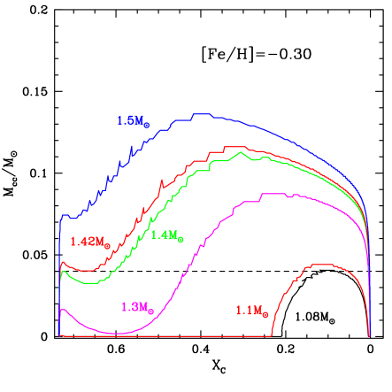
Figure 1: Convective core mass as a function of the central H mass fraction for stellar models with the labelled masses, and a metallicity Z=0.0077. The dashed line represents the value of $M_{cc}^{min}$ adopted in our calculations. In this example $M_{ov}^{inf}$=$1.08~{}M_{\odot}$ and $M_{ov}^{sup}$=$1.42~{}M_{\odot}$ (see text for details).

This criterion is obviously somehow arbitrary. It is based on numerical experiments we performed comparing the model predictions with empirical benchmarks such as eclipsing binaries and intermediate-age star clusters, as shown in Sect. 6. Our choice indirectly introduces a dependence of $M_{ov}^{inf}$ and $M_{ov}^{sup}$ on the initial metallicity (see Table 2). This is because the relationship between $M_{cc}^{min}$ and the total mass of the model depends on the efficiency of H-burning via the CNO-cycle, that in turn is affected by a change of the absolute value of the total CNO abundance.

The values of $M_{ov}^{inf}$ and $M_{ov}^{sup}$ for each initial chemical composition of our model grid are listed in Table 2. This approach is different from the previous BaSTI release where, regardless of the chemical composition, we fixed the overshoot efficiency to its maximum value (${\rm\lambda_{OV}}$=0.2) for initial masses larger than or equal to $1.7~{}M_{\odot}$, decreasing linearly down to zero when the initial mass is equal to ${\rm 1.1M_{\odot}}$.

Before closing this discussion, it is interesting to compare our recipe for decreasing ${\rm\lambda_{OV}}$ with decreasing initial mass, with the results of a recent calibration by Claret & Torres (2016). These authors compared their own model grid with effective temperatures and radii of a sample of detached double-lined eclipsing binaries with well determined masses, in the [Fe/H] range between about solar and $\sim-$1.01. They determined ${\rm\lambda_{OV}}$ equal to zero for masses lower than about $1.2M_{\odot}$, increasing to 0.2 in the mass range between $1.2M_{\odot}$ and $2M_{\odot}$. For masses larger than $2M_{\odot}$ ${\rm\lambda_{OV}}$ is equal to $\sim$0.2, as in our calculations. In the same metallicity range the value we adopt for $M_{ov}^{inf}$ ranges between $\sim$1.1 and $\sim 1.2M_{\odot}$, whereas $M_{ov}^{sup}$ is always equal to $\sim$1.4$M_{\odot}$, about $0.6M_{\odot}$ smaller than Claret & Torres (2016) result. It is however very difficult to compare the two sets of results. Apart from possible intrinsic differences in the models, Claret & Torres (2016) determine from their fits also the individual values of the mixing length for each component, the initial metallicity $Z$ of each system, and allowed age differences up to 5% between the components of each system. They derived often systematically lower metallicites than the corresponding spectroscopic measurements. In Sect. 6 we will see that our models fits well the mass-radius relationship of the systems KIC8410637 and OGLE-LMC-ECL-15260 (this latter also studied by Claret & Torres, 2016) whose masses are in the 1.3-1.5 $M_{\odot}$ range, bracketing the upper limit where ${\rm\lambda_{OV}}$ reached 0.2 with our calibration. We have imposed in our comparisons equal age for both systems, no variation of the mixing length and used models with chemical composition consistent with the spectroscopic measurements.

In case of core He-burning of low- and intermediate-mass stars, we model core mixing with the semiconvective formalism by Castellani et al. (1985), and breathing pulses inhibited following Caputo et al. (1989). During core He-burning in massive stars, we use the Schwarzschild criterion without overshooting to fix the boundary of the mixed region.

We do not include overshooting from the lower boundaries of convective envelopes.

2.3 Radiative and electron conduction opacities

The sources for the radiative Rosseland opacity are the same as for the previous BaSTI calculations. More in detail, opacities are from the OPAL calculations (Iglesias & Rogers, 1996) for temperatures larger than ${\rm\log(T)=4.0}$, whereas calculations by Ferguson et al. (2005) – including contributions from molecules and grains – have been adopted for lower temperatures. Both high- and low-temperature opacity tables have been computed for the solar scaled heavy element distribution listed in Table 1.

As for the electron conduction opacities, at variance with the models presented in Pietrinferni et al. (2004, 2006), we have now adopted the results by Cassisi et al. (2007). As shown by Cassisi et al. (2007), these opacity calculations affect only slightly (small decrease) the He-core mass at He-ignition for low-mass models, and the luminosity of the folllwing horizontal branch (HB) phase (small decrease), compared to the BaSTI calculations that were based on the Potekhin (1999) conductive opacities. For more details on this issue we refer the reader to the quoted reference as well as to Serenelli et al. (2017).

2.4 Equation of state

As in Pietrinferni et al. (2004) we use the detailed EOS by A. Irwin. A brief discussion of the characteristics of this EOS can be found in Cassisi et al. (2003). We recomputed all required EOS tables for the heavy element distribution in Table 1 adopting the option ‘EOS1’ in Irwin’s code. This option –recommended by A. Irwin (see also the discussion in Cassisi et al., 2003)– provides the best match to the OPAL EOS (Rogers & Nayfonov, 2002a), and Saumon et al. (1995a) EOS in the low-temperature and high-density regime.

2.5 Nuclear reaction rates

The nuclear reaction rates are from the NACRE compilation (Angulo et al., 1999), with the exception of the three following reactions, whose rates come from recent reevaluations:

• ${\rm{}^{3}He(^{4}He,\gamma)^{7}Be}$ - Cyburt & Davids (2008);

• ${\rm{}^{14}N(p,\gamma)^{15}O}$ - Formicola et al. (2004);

• ${\rm{}^{12}C(\alpha,\gamma)^{16}O}$ - Hammer et al. (2005).

The previous BaSTI calculations employed the NACRE rates (Angulo et al., 1999) for all reactions with the exceptions of the ${\rm{}^{12}C(\alpha,\gamma)^{16}O}$ rate taken from Kunz et al. (2002)

The first two reaction rates are important for H-burning; indeed the ${\rm{}^{14}N(p,\gamma)^{15}O}$ reaction is crucial among those involved in the CNO-cycle, because it is the slowest one. The impact of this recent ${\rm{}^{14}N(p,\gamma)^{15}O}$ rate on stellar evolution models has been investigated by Imbriani et al. (2004), Weiss et al. (2005) and Pietrinferni et al. (2010). However, we have repeated here the analysis to verify the expected variation with respect to the previous BaSTI calculations, due to the combined effects of using the new rates for both ${\rm{}^{3}He(^{4}He,\gamma)^{7}Be}$ and ${\rm{}^{14}N(p,\gamma)^{15}O}$ nuclear reactions. When all other physics inputs are kept fixed, we have found that:

• for a ${\rm 0.8M_{\odot}}$, Z=0.0003 model, the luminosity at the MS turn-off (TO) increases by $\Delta\log(L/L_{\odot})\sim 0.02$, while the age increases by about 210 Myr when passing from the NACRE reaction rates used in the previous BaSTI calculations to the ones adopted for the new models. For the same mass but a metallicity Z=0.008 the effects are smaller, with a MS TO luminosity increased by about 0.01 dex and an age increased by $\sim 30$ Myr;

• as for the evolution along the red giant branch (RGB), the effect of the new rates on the RGB bump luminosity is completely negligible at Z=0.008, while the RGB bump luminosity increases by $\Delta\log(L/L_{\odot})\sim 0.04$ at Z=0.0003. Regardless of the metallicity, the use of the new rates decreases the RGB tip brightness by $\Delta\log(L/L_{\odot})\sim 0.02$ in agreement with the results by Pietrinferni et al. (2010) and Serenelli et al. (2017).

The ${\rm{}^{12}C(\alpha,\gamma)^{16}O}$ reaction is one of the most critical nuclear processes in stellar astrophysics, because of its impact on a number of astrophysical problems (see, e.g., Cassisi et al., 2003; Cassisi & Salaris, 2013, and references therein). The more recent assessment of this reaction rate is not significantly different from Kunz et al. (2002) as used by Pietrinferni et al. (2004). As a consequence, the use of this new rate has a small impact on the models: For instance, the core He-burning lifetime is decreased by a negligible $\sim 0.2$% when using this new rate compared to models calculated with the older Kunz et al. (2002) rate.

As in the previous BaSTI calculations, electron screening is calculated according to the appropriate choice between strong, intermediate, and weak, following Dewitt et al. (1973) and Graboske et al. (1973).

2.6 Neutrino energy losses

Neutrino energy losses are included with the same prescriptions as in the previous BaSTI calculations. For plasma neutrinos we use the rates by Haft et al. (1994), supplemented by Munakata et al. (1985) rates for the other relevant neutrino production processes.

2.7 Superadiabatic convection and outer boundary conditions

The combined effect of the treatment of the superadiabatic layers of convective envelopes, and the method to determine the outer boundary conditions of the models, has a major impact on the effective temperature scale of stellar models with deep convective envelopes (or fully convective).

As in the previous BaSTI models, we treat the superadiabatic convective layers according to the Böhm-Vitense (1958) flavor of the mixing length theory, using the formalism by Cox & Giuli (1968). The value of the mixing length parameter ${\rm\alpha_{ML}}$ is fixed by the solar model calibration to 2.006 (see Sect. 3 for more details) and kept the same for all masses, initial chemical compositions and evolutionary phases.

Regarding the outer boundary conditions, in the previous BaSTI models they were obtained by integrating the atmospheric layers employing the $T(\tau)$ relation provided by Krishna Swamy (1966). In this new release we decided to employ the alternative solar semi-empirical $T(\tau)$ by Vernazza et al. (1981). More specifically, we implemented in our evolutionary code the following fit to the tabulation provided by Vernazza et al. (1981):

$$T^{4}=0.75\ T_{eff}^{4}\ (\tau+1.017-0.3e^{-2.54\tau}-0.291e^{-30\tau})$$ (1)

As shown by Salaris & Cassisi (2015), model tracks computed with this $T(\tau)$ relation approximate well results obtained using the hydro-calibrated $T(\tau)$ relationships determined from the 3D radiation hydrodynamics calculations by Trampedach et al. (2014) for the solar chemical composition. Figure 2 shows the Hertzsprung-Russell diagram (HRD) of $0.85~{}M_{\odot}$ evolutionary tracks from the pre-MS to the tip of the RGB, computed for three labelled initial metallicities. The physics inputs are kept the same as the old BaSTI calculations, but for the $T(\tau)$ relation, that is either from Krishna Swamy (1966) or Vernazza et al. (1981). For both choices the value of ${\rm\alpha_{ML}}$ has been fixed by an appropriate solar calibration.

The two sets of models overlap almost perfectly along the MS at all $Z$, whereas some differences in $T_{eff}$ at fixed luminosity appear along the RGB (and the pre-MS). Differences are of about 60 K at the lowest metallicity, reaching $\sim 90$ K at solar metallicity. Tracks calculated with the Vernazza et al. (1981) $T(\tau)$ are always the cooler ones. For a more detailed discussion on the impact of different $T(\tau)$ relations on the $T_{eff}$ scale of RGB stellar models we refer to Salaris & Cassisi (2015) and references therein.

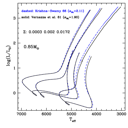
Figure 2: HRDs of models computed with two different assumptions about the $T(\tau)$ relation used to calculate the outer boundary conditions, for the labelled mass and metallicities. The solar calibrated mixing length values for each choice of the $T(\tau)$ relation are also shown.

In the first release of BaSTI the minimum stellar mass was set to $0.50~{}M_{\odot}$ for all chemical compositions, while these new calculations include the mass range below $0.50~{}M_{\odot}$, down to $0.10~{}M_{\odot}$. As extensively discussed in the literature (see, e.g., Baraffe et al., 1995; Allard et al., 1997; Brocato et al., 1998; Chabrier & Baraffe, 2000, and references therein) in this regime of so-called very low-mass (VLM) stars, i.e. ${\rm M\leq 0.45M_{\odot}}$, outer boundary conditions provided by accurate non-gray model atmospheres are required. Therefore for the VLM model calculations we employed boundary conditions (pressure and temperature at a Rosseland optical depth $\tau$=100) taken from the PHOENIX model atmosphere library (Allard et al., 2012, and references therein), more precisely the BT-Settl model set. These model atmospheres properly cover the required parameter space in terms of effective temperature, surface gravity and metallicity range. However, this set of models have been computed for the Asplund et al. (2009) solar heavy element distribution, that is different from the one adopted in our calculations (see Sect. 2.1).

One could argue that this difference in the heavy element mixture may have an impact on the predicted spectral energy distribution, but it should have only a minor effect on the model atmosphere structure, hence on the derived outer boundary conditions. We have verified this latter point as follows. The PHOENIX model atmosphere repository contains a subset of models –labelled CIFIST2011 – computed with the same solar heavy element distribution as in our calculations (Caffau et al., 2011), for a few selected metallicities. We have calculated sets of VLM models using alternatively the PHOENIX boundary conditions for the Asplund et al. (2009) mixture and the Caffau et al. (2011) one. Figure 3 shows the result of such comparison for one selected metallicity. As expected the the two sets of VLM calculations provide very similar HRDs. Differences in bolometric luminosity and effective temperature are vanishing small for masses larger than $\sim 0.12~{}M_{\odot}$, while they are equal to just $\Delta\log(L/L_{\odot})\sim 0.007$ and $\Delta{T_{eff}}\sim 16$ K, for smaller masses.

We close this section with more details about the transition from VLM models with outer boundary conditions determined from PHOENIX model atmospheres, to models calculated with the $T(\tau)$ relation in Eq. 1. To achieve a smooth transition in the $log(L/L_{\odot})-T_{eff}$ diagram between the two regimes, for each chemical composition we computed models with mass up to $0.70~{}M_{\odot}$ with the PHOENIX boundary conditions, and models with mass down to $0.4~{}M_{\odot}$ using the $T(\tau)$ relation. In the overlapping mass range we selected a specific transition mass corresponding to the pair of models –that happen to fall in the range between $\sim~{}0.5M_{\odot}$ and $\sim 0.65~{}M_{\odot}$, depending on the initial composition– showing negligible differences in both bolometric luminosity and effective temperature, typically $\Delta{T_{eff}}\leq 25$ K, and $\Delta\log(L\L_{\odot})\leq 0.004$. For masses equal and lower than this mass we keep the calculations with PHOENIX boundary conditions, and above this limit the models with $T(\tau)$ integration. This allows to calculate isochrones displaying a smooth transition between the two boundary condition regimes.

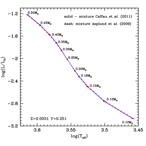
Figure 3: HRD of core H-burning models for an age of 10 Gyr and the labelled initial chemical composition and masses. Boundary conditions have been obtained from model atmospheres calculated using the labelled solar heavy element mixtures (see text for details).

2.8 Mass loss

Mass loss is included with the Reimers (1975) formula, as in the previous BaSTI models. The free parameter $\eta$ entering this mass loss prescription has been set equal to 0.3, following the Kepler observational constraints discussed in Miglio et al. (2012a). We provide also stellar models computed without mass loss ($\eta$=0). The previous BaSTI calculations included three options, $\eta$=0, 0.2 and 0.4, respectively.

3 The Standard Solar Model

As already mentioned, the calibration of the SSM sets the value of ${\rm\alpha_{ML}}$, and the initial solar He abundance and metallicity. At the solar age ($t_{\odot}=4.57$ Gyr Bahcall et al., 1995) our $1~{}M_{\odot}$ SSM (including diffusion of both He and metals and calculated starting from the pre-main sequence) matches luminosity, radius ($L_{\odot}=3.842\times 10^{33}$ erg/s and $R_{\odot}=6.9599\times 10^{10}$ cm, respectively, as given by Bahcall et al., 1995), and the present ($Z/X$)_⊙ (Caffau et al., 2011) abundance ratio with initial abundances $Z^{\rm ini}_{\odot}=0.01721$ and $Y^{\rm ini}_{\odot}=0.2695$, and mixing length ${\rm\alpha_{ML}=2.006}$.

Our SSM has a surface He abundance $Y_{\rm\odot,surf}=$0.238 and a radius of the boundary of the surface convective zone $R_{\rm CZ}/R_{\odot}$ equal to 0.722. These values have to be compared with the asteroseismic estimates $R_{\rm CZ}/R_{\odot}=0.713\pm 0.001$ (Basu, 1997) and $Y_{\rm\odot,surf}=0.2485\pm 0.0035$ (Basu & Antia, 2004). These differences between models and observations are common to all SSMs based on the revised solar surface compositions discussed before (e.g. Basu & Antia, 2004; Vinyoles et al., 2017, and references therein). Differences are larger when using the lower $Z$ solar abundances by Asplund et al. (2009), as discussed by Choi et al. (2016). This is an open problem, and efforts are being devoted to explore the possibility of suitable changes to the SSM input physics, such as radiative opacities (we refer to Villante, 2010; Krief et al., 2016; Vinyoles et al., 2017, for a detailed analysis of this issue).

4 The stellar model library

Our new model library increases significantly the number of available metallicities, compared to the old BaSTI calculations. We have calculated models for 22 metallicities ranging from $Z=10^{-5}$ up to $\sim 0.04$; the exact values are listed in Table 2. We adopted a primordial He abundance $Y=0.247$ based on the cosmological baryon density following Planck results (Coc et al., 2014). With this choice of the primordial He abundance and the initial solar He abundance obtained from the SSM calibration we obtain an He-enrichment ratio d$Y$/d$Z$=1.31, that we have used in our model grid computation. For each metallicity, the corresponding initial He abundance and [Fe/H] are listed in Table 2.

4.1 Evolutionary tracks

As with the first release of the BaSTI database, we have calculated several model grids by varying once at a time some modelling assumptions. A schematic overview of all grids made available in the new BaSTI repository is provided in Table 3. Our reference set of models is set a) in Table 3, that include main sequence convective core overshooting, mass loss with $\eta$=0.3 and atomic diffusion of He and metals.

For each chemical composition (and choice of modelling assumptions) we have computed 56 evolutionary sequences. The minimum initial mass is $0.1~{}M_{\odot}$, while the maximum value is $15~{}M_{\odot}$). For initial masses below $0.2~{}M_{\odot}$ we computed evolutionary tracks for masses equal to 0.10, 0.12, 0.15 and $0.18~{}M_{\odot}$. In the range between 0.2 and $0.7~{}M_{\odot}$ a mass step equal to $0.05~{}M_{\odot}$ has been adopted. Mass steps equal to $0.1~{}M_{\odot}$, $0.2~{}M_{\odot}$, 0.5 $M_{\odot}$ and 1 $M_{\odot}$ have been adopted for the mass ranges $0.7-2.6~{}M_{\odot}$, $2.6-3.0~{}M_{\odot}$, $3.0-10.0~{}M_{\odot}$, and masses larger than $10.0M_{\odot}$, respectively.

Models less massive than $4.0~{}M_{\odot}$ have been computed from the pre-MS, whereas more massive models have been computed starting from a chemically homogeneous configuration on the MS. Relevant to pre-MS calculations, the adopted mass fractions for D, ${\rm{}^{3}He}$ and ${\rm{}^{7}Li}$ are equal to $3.9\ 10^{-5}$, $2.3\ 10^{-5}$, and $2.6\ 10^{-9}$ respectively.

All stellar models – but the less massive ones whose core H-burning lifetime is longer than the Hubble time – have been calculated until the start of the thermal pulses (TPs) on the Asymptotic Giant Branch (AGB), or C-ignition for the more massive ones. For the long-lived low-mass models we have stopped the calculations when the central H mass fraction is $\sim$0.3 (corresponding to ages already much larger than the Hubble time).

For each initial chemical composition we provide also an extended set of core He-burning models suited to study the HB in old stellar populations. We have considered various values of the total mass (with a fine mass spacing, as in Pietrinferni et al., 2004) but the same mass for the He-core and the same envelope chemical stratification, corresponding to a RGB progenitor at the He-flash for an age of $\sim 12.5$ Gyr.

All evolutionary tracks presented in this work have been reduced to the same number of points (‘normalized’) to calculate isochrones (see, e.g., Dotter, 2016, for a discussion on this issue) and for ease of interpolation, by adopting the same approach extensively discussed in Pietrinferni et al. (2004) and updated in Pietrinferni et al. (2006). This method is based on the identification of some characteristic homologous points (keypoints) corresponding to well-defined evolutionary stages along each individual track (see Pietrinferni et al., 2004, for more details on this issues). Given that almost all the evolutionary tracks now include the pre-MS stage, we added three additional keypoints compared to the previous BaSTI calculations. The first one is taken at an age of $10^{4}$ yr, the second one corresponds to the end of the deuterium burning stage, while the third keypoint is set at the first minimum of the surface luminosity for all models but the VLM ones. For these latter masses this point corresponds to the stage when the energy produced by the p-p chain starts to dominate the energy budget. The fourth keypoint corresponds to the zero age main sequence (ZAMS) defined as the model fully sustained by nuclear reactions, with all secondary elements at their equilibrium abundances. However, for VLM models that attain nuclear equilibrium of the secondary elements involved in the p-p chain over extremely long timescales, this keypoint corresponds to the first minimum of the bolometric luminosity. All subsequent keypoints are fixed exactly as in the previous BaSTI database. Table 4 lists the correspondence between keypoints and evolutionary stages as well as the corresponding line number in the normalized evolutionary track, while Fig. 4 shows the location of a subset of keypoints (the first ten ones) on selected evolutionary tracks.

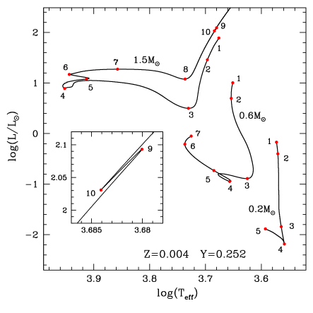
Figure 4: HRD of selected evolutionary tracks and the labelled initial chemical composition. We also show the position of the first 10 key points used to normalize the tracks. The inset is an enlargement of the RGB bump phase, to show the exact position of key points 9 and 10.

For each chemical compositions, these normalized evolutionary tracks are used to compute extended sets of isochrones for ages between 20 Myr and 14.5 Gyr (older isochrones can be also computed on demand).

Table 2: Grid of initial chemical abundances and corresponding values (in solar masses) of $M_{ov}^{inf}$ and $M_{ov}^{sup}$ (see text for details).

$Z$	$Y$	[Fe/H]	$M_{ov}^{inf}$	$M_{ov}^{sup}$
0.00001	0.2470	$-3.20$	1.30	2.09
0.00005	0.2471	$-2.50$	1.30	1.78
0.00010	0.2471	$-2.20$	1.30	1.68
0.00020	0.2472	$-1.90$	1.30	1.59
0.00031	0.2474	$-1.70$	1.30	1.54
0.00044	0.2476	$-1.55$	1.30	1.50
0.00062	0.2478	$-1.40$	1.32	1.47
0.00079	0.2480	$-1.30$	1.32	1.45
0.00099	0.2483	$-1.20$	1.24	1.44
0.00140	0.2488	$-1.05$	1.21	1.43
0.00197	0.2496	$-0.90$	1.17	1.42
0.00311	0.2511	$-0.70$	1.13	1.42
0.00390	0.2521	$-0.60$	1.10	1.42
0.00614	0.2550	$-0.40$	1.09	1.42
0.00770	0.2571	$-0.30$	1.08	1.42
0.00964	0.2596	$-0.20$	1.08	1.42
0.01258	0.2635	$-0.08$	1.08	1.43
0.01721	0.2695	$0.06$	1.09	1.43
0.02081	0.2742	$0.15$	1.11	1.47
0.02865	0.2844	$0.30$	1.10	1.42
0.03905	0.2980	$0.45$	1.09	1.40

Table 3: The various grids of stellar models provided in the database.

Case	Convective overshooting	Mass loss efficiency	Diffusion
a	Yes	$\eta=0.3$	Yes
b	Yes	$\eta=0.3$	No
c	Yes	$\eta=0.0$	No
d	No	$\eta=0.0$	No

Table 4: Correspondence between evolutionary stage, key point and line number of the normalized tracks.

Key Point	Line	Evolutionary Phase
1	1	Age equal to 1000 yr
2	20	End of deuterium burning
3	60	The first minimum in the surface luminosity, or when nuclear energy starts to dominate the energy budget
4	100	Zero age main sequence or minimum in bolometric luminosity for VLM models
5	300	First minimum of $T_{eff}$ for high-mass or central H mass fraction $X_{c}$=0.30 for low-mass and VLM models
6	360	Maximum in $T_{eff}$ along the MS (TO point)
7	420	Maximum in $\log(L/L_{\odot})$ for high-mass or $X_{c}$=0.0 for low-mass models
8	490	Minimum in $\log(L/L_{\odot})$ for high-mass or base of the red giant branch for low-mass models
9	860	Maximum luminosity along the RGB bump
10	890	Minimum luminosity along the RGB bump
11	1290	Tip of the RGB
12	1300	Start of quiescent core He-burning
13	1450	Central abundance of He equal to 0.55
14	1550	Central abundance of He equal to 0.50
15	1650	Central abundance of He equal to 0.40
16	1730	Central abundance of He equal to 0.20
17	1810	Central abundance of He equal to 0.30
18	1950	Central abundance of He equal to 0.00
19	2100	The energy associated to the CNO-cycle becomes larger than that provided by He-burning

Figure 5 shows an example of the full set of reference tracks and isochrones calculated for one chemical composition (Y=0.2695, Z=0.01721). Panel $a$ displays the full grid of tracks for masses ranging from 0.1$M_{\odot}$ to 15$M_{\odot}$, while panel $c$ focuses on the RGB region for a subset of models with mass between 0.4 and 4.5$M_{\odot}$ (dotted lines denote the pre-MS evolution of the same models). The set of HB tracks is shown in panel $d$, for a RGB progenitor mass equal to 1.0$M_{\odot}$, and minimum HB mass equal to 0.4727$M_{\odot}$, while panel $e$ displays a subset of pre-MS, MS and RGB tracks with mass between 0.1 a 1.0$M_{\odot}$. Finally, panel $b$ displays a set of isochrones with ages equal to 20 Myr, 100 Myr, 500 Myr, 1 Gyr, 4 Gyr and 14 Gyr, respectively (solid lines), overlaid onto the full set of tracks (dashed lines).

Figure 5: HRDs of the full set of reference tracks and isochrones calculated for the labelled initial chemical composition (panel $a$), and a subset of isochrones for 5 Myr (long dashed line), and 20 Myr, 100 Myr, 500 Myr, 1 Gyr, 4 Gyr and 14 Gyr, solid lines in panel $b$) overlaid onto the track grid (dashed lines). Panel $c$ shows selected RGB tracks (solid lines) and part of their pre-MS evolution (dotted lines), while panel $d$ displays the full set of HB tracks. The zero age HB is shown as a dotted line, while the dashed line corresponds to central He exhaustion. Panel $e$ displays a subset of pre-MS (dotted), MS and RGB tracks with mass between 0.1 a 1.0 $M_{\odot}$ (see text for details).

4.2 Bolometric corrections

Bolometric luminosities and effective temperatures along evolutionary tracks and isochrones need to be translated to magnitudes and colors in sets of photometric filters, for comparisons with observed color-magnitude-diagrams (CMDs), and to predict integrated fluxes of unresolved stellar populations. This requires sets of stellar spectra covering the relevant parameter space in terms of metallicity, surface gravity and effective temperature of the models. For such aim, a new grid of model atmospheres has been computed using the latest version of the ATLAS9 code originally developed by R. L. Kurucz (Kurucz, 1970). ATLAS9 allows to calculate one-dimensional, plane-parallel model atmospheres under the assumption of local thermodynamical equilibrium for all the species. The method of the opacity distribution function (ODF – Kurucz et al., 1974) is employed to handle the line opacity, by pretabulating the line opacity as a function of gas pressure and temperature in a given number of wavelength bins. ODFs and Rosseland mean opacity tables are calculated for a given metallicity (fixing the chemical mixture) and for a given value of microturbulent velocity. Even if the computation of ODFs can be time consuming, the calculation of any model atmosphere (defined by its effective temperature and gravity) for the metallicity and microturbulent velocity corresponding to the adopted ODF turns out to be very fast.

Grids of ATLAS9 model atmospheres based on suitable ODFs are freely available but based on different solar chemical abundances compared to the one used in our calculations. The grid by Castelli & Kurucz (2004) adopted the solar abundances by Grevesse & Sauval (1998), that computed by Kirby (2011) the abundances by Anders & Grevesse (1989), while the recent one by Mészáros et al. (2012) for the APOGEE survey used the abundances by Asplund et al. (2005). For the new grid presented here we adopted the same solar metal distribution of the stellar evolution calculations. For the computation of new ODFs, Rosseland opacity tables and model atmospheres we followed the scheme described in Mészáros et al. (2012).

For each [Fe/H] and microturbulent velocity, one ODF and one Rosseland opacity table are calculated using the codes DFSYNTHE and KAPPA9 (Castelli, 2005), respectively. The [Fe/H] grid ranges from $-$4.0 to +0.5 dex in steps of 0.5 dex from $-$4.0 to $-$3.0 dex, and in steps of 0.25 dex for the other metallicities, assuming solar scaled abundances for all elements. The adopted values for the microturbulent velocities are 0, 1, 2, 4 and 8 km/s. In the calculation of the ODFs we included all atomic and molecular transitions listed in F. Castelli website; in particular the linelist for TiO is from Schwenke (1998) and that for ${\rm H_{2}O}$ is from Langhoff et al. (1997).

For each [Fe/H] (but adopting only the microturbulent velocity of 2 km/s) a grid of ATLAS9 model atmospheres has been computed, covering the effective temperature-surface gravity parameter space summarized in Table 5, for a total of 475 models.

Similarly to those computed by Castelli & Kurucz (2004), these new model atmospheres include 72 plane-parallel layers ranging from $\log{\tau}$=$-$6.875 (where $\tau$ is the Rosseland optical depth) to +2.00, in steps of 0.125, and have been computed with the overshooting option switched off, adopting a mixing-length equal to 1.25 as previous calculations. For each model atmosphere, the corresponding emerging flux has been then computed.

Table 5: Effective temperature and surface gravity ranges covered by our new grid of ATLAS9 model atmospheres and spectra, together with the grid spacings $\Delta_{T_{eff}}$ and $\Delta_{log(g)}$.

$T_{eff}$	$\Delta_{T_{eff}}$	log(g)	$\Delta_{\rm log(g)}$
(K)	(K)	(c.g.s)	(c.g.s)
3500–6000	250	0.0–5.0	0.5
6250–7500	250	0.5–5.0	0.5
7750–8250	250	1.0–5.0	0.5
8500–9000	250	1.5–5.0	0.5
9250–11750	250	2.0–5.0	0.5
12000–13000	250	2.5–5.0	0.5
13000–19000	1000	2.5–5.0	0.5
20000–26000	1000	3.0–5.0	0.5
27000–31000	1000	3.5–5.0	0.5
32000–39000	1000	4.0–5.0	0.5
40000–49000	1000	4.5–5.0	0.5
50000	—	5.0	—

The ATLAS9 grid of spectra is complemented by two addiitonal spectral libraries, to cover the parameter space of cool giants and low-mass dwarfs. At low ${\rm T_{eff}}$ and surface gravities, we use the BaSeL WLBC99 results (Westera et al., 1999, 2002). This is a semi-empirical library, built from a grid of theoretical spectra that have been later calibrated to match empirical color-$T_{eff}$ relations from neighborhood stars. These templates are available in the metallicity range ${\rm-2.0\leq[Fe/H]\leq 0.5}$, in steps of 0.5 dex. For the low $T_{eff}$ and high gravity regime, we use spectra from the Göttingen Spectral Library (Husser et al., 2013). These have been calculated using the code PHOENIX (Hauschildt & Baron, 1999), which is particularly suited to model atmospheres of cool dwarfs. The PHOENIX configuration used for this library employs a variable parametrization of microturbulence and mixing length, depending on the properties of the modelled atmosphere. The metallicity coverage is ${\rm-4.0\leq[Fe/H]\leq 1.0}$, in steps of 0.5 dex. Figure 6 shows the range of effective temperature and surface gravity covered by our adopted spectral libraries.

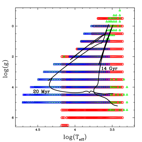
Figure 6: The $T_{eff}-$ log(g) coverage ([Fe/H] = 0) of the adopted spectral libraries. Different symbols correspond to our ATLAS9 grid (blue diamonds), the WLBC99 (green triangles), and the Göttingen (red circles) spectral libraries. Two solar metallicity isochrones for 20 Myr and 14 Gyr are also shown.

We have computed tables of bolometric corrections (BCs) for several popular photometric systems (the complete list is found in Table 6), following the prescription by Girardi et al. (2002) for photon-counting defined systems:

$$BC_{S_{\lambda}}=M_{bol,\odot}-2.5\log{\Bigl{[}4\pi(10pc)^{2}F_{bol}/L_{\odot}\Bigr{]}}$$

$$+2.5\log{\Biggl{(}\frac{\int_{\lambda_{1}}^{\lambda_{2}}\lambda F_{\lambda}S_{\lambda}d\lambda}{\int_{\lambda_{1}}^{\lambda_{2}}\lambda f^{0}_{\lambda}S_{\lambda}d\lambda}\Biggr{)}}-m^{0}_{S_{\lambda}}$$ (2)

where $S_{\lambda}$ is a generic filter response curve, defined between $\lambda_{1}$ and $\lambda_{2}$, $F_{bol}=\sigma T_{eff}^{4}$ is the total emerging flux at the stellar surface, $F_{\lambda}$ is the stellar emerging flux at a given wavelength, $f^{0}_{\lambda}$ is the wavelength-dependent flux of a reference spectrum and $m^{0}_{S_{\lambda}}$ is the magnitude of the reference spectrum in the filter $S_{\lambda}$ (denoted as zero point). We adopt $M_{bol,\odot}=4.74$, following the IAU B2 resolution of 2015 (Mamajek et al., 2015).

The reference spectra are either the spectrum of Vega ($\alpha\ Lyr$), for systems that use Vega for the magnitude zero points (Vegamag systems), or a spectrum with constant flux density per unit frequency $f^{0}_{\nu}=3.631\cdot 10^{-20}{\rm erg\,s^{-1}\,cm^{-2}\,Hz^{-1}}$, for ABmag systems. For older photometric systems, such as the Johson-Cousins-Glass UBVRIJHKLM we use the energy-integration equivalent of Eq. 2.

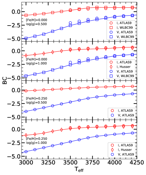
Figure 7: An example of our final BC set (solid lines) for the V and I photometric passbands, as a function of the effective temperature, for some selected metallicities and surface gravities (see text for details).

Table 6: Available photometric systems. We also list the source for the passband definitions and reference zero-points.

Photometric system	Calibration	Passbands	Zero-points
UBVRIJHKLM	Vegamag	Bessell & Brett (1988); Bessell (1990)	Bessell et al. (1998)
HST - WFPC2	Vegamag	SYNPHOT	SYNPHOT
HST - WFC3	Vegamag	SYNPHOT	SYNPHOT
HST - ACS	Vegamag	SYNPHOT	SYNPHOT
2MASS	Vegamag	Cohen et al. (2003)	Cohen et al. (2003)
DECam	ABmag	DES collaboration	0
Gaia	Vegamag	Jordi et al. (2010)	Jordi et al. (2010)
JWST - NIRCam	Vegamag	JWST User Documentation	SYNPHOT
SAGE	ABmag	SAGE collaboration	0
Skymapper	ABmag	Bessell et al. (2011)	0
Sloan	ABmag	Fukugita et al. (1996)	Dotter et al. (2008)
Strömgren	Vegamag	Maíz Apellániz (2006)	Maíz Apellániz (2006)
VISTA	Vegamag	ESO	González-Fernández et al. (2017)

Due to the differences between the adopted sets of spectral libraries, the resulting BCs display non-negligible differences in the overlapping ${\rm T_{eff}}$ and surface gravity regimes. To eliminate discontinuities in the final merged BC set, the different sets were matched smoothly in the overlapping regions by applying some suitable ramping at the edge of the various tables. After several tests we adopted the following combination of BC libraries:

• at metallicities equal or lower than solar, for the V passband (or passbands with equivalent effective wavelengths) and all photometric passbands bluer than the V-band we employ the BCs from our ATLAS9 grid, supplemented at lower gravities and $T_{eff}<3900$ K by WLBC99 results. For redder passbands and $T_{eff}<3900$ K we switch at ${\rm\log(g)=1.0}$ from our ATLAS9 BCs to Husser et al. (2013) BCs for higher gravities, and to WLBC99 BCs for lower gravities;

• at super solar metallicities, we adopt our ATLAS9 BCs for the V band (or equivalent) as well as for bluer photometric passbands, extrapolating linearly in log(g) and $T_{eff}$ when necessary. For redder photometric passbands we use ATLAS9 BCs for gravities lower than ${\rm\log(g)=1.0}$ (extrapolated when necessary) and Husser et al. (2013) BCs for gravities larger or equal than this limit, and $T_{eff}<3900$ K.

Figure 7 shows examples of our adopted composite BC library.

4.3 Asteroseismic properties of the models

Asteroseismology has experienced a revolution thanks to past and present space missions such as CoRoT (Baglin et al., 2009), Kepler (Gilliland et al., 2010b), and K2 (Chaplin et al., 2015), which have provided high-precision photometric data for hundreds of main-sequence and sub-giant stars and for thousands of red giants.

Future satellites like TESS (Ricker et al., 2014) and PLATO (Rauer et al., 2014) hold promises to expand the current sample greatly and thus further extend the impact of asteroseismology in the fields of stellar physics (e.g., Beck et al., 2011; Verma et al., 2014), exoplanet studies (Huber et al., 2013; Silva Aguirre et al., 2015, e.g.,), and Galactic archaeology (e.g., Casagrande et al., 2016; Silva Aguirre et al., 2017). Given the availability of high-quality oscillations data, we provide the corresponding theoretical quantities to fully exploit their potential.

We have computed adiabatic oscillation frequencies for all the models using the Aarhus aDIabatic PuLSation package (ADIPLS, Christensen-Dalsgaard, 2008). We provide the radial, dipole, quadrupole, and octupole mode frequencies for the models with central hydrogen mass fraction $>10^{-4}$ and only the radial mode frequencies for more evolved models. The power spectrum of the solar-like oscillators have several global characteristic features that can be used to constrain the stellar properties. Some of these features do not require very high signal-to-noise data for their determinations –in contrast to the individual oscillation frequencies which need long time-series data with high signal-to-noise ratio for their measurements - and play a crucial role in ensemble studies. We also provide three such global asteroseismic quantities for the models, viz., the frequency of maximum power ($\nu_{\rm max}$), large frequency separation for the radial mode frequencies ($\Delta\nu_{0}$), and the asymptotic period spacing for the dipole mode frequencies ($\Delta P_{1}$).

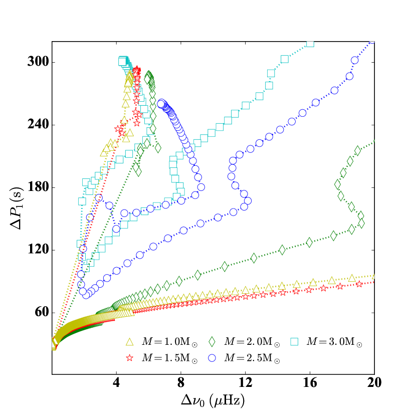
Figure 8: Asymptotic period spacing as a function of the large frequency separation for a set of 5 tracks with different masses and teh same initial composition ($Y=0.26$ and $[{\rm Fe}/{\rm H}]=-0.2$ dex).

The value of $\nu_{\rm max}$ was determined using the well known scaling relation (Kjeldsen & Bedding, 1995),

$$\frac{\nu_{\rm max}}{\nu_{{\rm max},\odot}}=\left(\frac{M}{M_{\odot}}\right)\left(\frac{R}{R_{\odot}}\right)^{-2}\left(\frac{T_{\rm eff}}{T_{{\rm eff},\odot}}\right)^{-1/2},$$ (3)

where $M$, $R$, and $T_{\rm eff}$ are the model mass, radius, and effective temperature, respectively. We adopted $\nu_{{\rm max},\odot}=3090~{}\mu$Hz from Huber et al. (2011), $T_{{\rm eff},\odot}=5777$ K, and $M_{\odot}=1.9891\times 10^{33}$ gm and $R_{\odot}=6.9599\times 10^{10}$ cm as used in the corresponding stellar tracks. We extracted $\Delta\nu_{0}$ following White et al. (2011), i.e., performing a weighted linear least squares fit to the radial mode frequencies as a function of the radial order, with a Gaussian weighting function centered around $\nu_{\rm max}$, with $0.25\,\nu_{\rm max}$ full width at half maximum. The large frequency separation and frequency of maximum power, together with the measurement of the stellar $T_{eff}$, have been used to determine masses and radii of large samples of isolated stars, independent of modelling, thus providing strong constraints on stellar evolution models and on models of Galactic stellar populations (see, e.g., Kallinger et al., 2010; Chaplin et al., 2011; Miglio et al., 2012b).

We determined the period spacing $\Delta P_{1}$ using the asymptotic expression,

$$\Delta P_{1}=\sqrt{2}\pi^{2}\left(\int\frac{N}{r}dr\right)^{-1},$$ (4)

where $N$ and $r$ are the Brunt-Väisälä frequency and radial coordinate, respectively. The integration is performed over the radiative interior. Since $N$ is weighted with $r^{-1}$ in the integral, $\Delta P_{1}$ is very sensitive to the Brunt-Väisälä frequency profile in the core. Hence the measurement of $\Delta P_{1}$ offers a unique opportunity to constrain the uncertain aspects of the physical processes taking place in stellar cores. As an example, Degroote et al. (2010) used the measurement of the period spacing for the star HD 50230 observed using the CoRoT satellite, to constrain the mixing in its core (see also, Montalbán et al., 2013). Figure 8 illustrates the evolution of models in the $\Delta\nu_{0}-\Delta P_{1}$ diagram (evolution proceeds from right to left). This is an interesting diagram because $\Delta\nu_{0}$ contains information mostly about the envelope, whereas $\Delta P_{1}$ about the core. The hook-like feature on the right (beyond the displayed range for ${\rm M=1.0}$ and 1.5 ${\rm M_{\odot}}$) correspond to the base of the red giant branch. The sudden jump at the lowest $\Delta\nu_{0}$ for ${\rm M=}$ 1.0, 1.5, and 2.0 ${\rm M_{\odot}}$ is due to the helium flash, which causes the stellar structure to change rapidly in a short period of time. This diagram have been used successfully to distinguish the shell hydrogen burning red giant stars with those that are fusing helium in the core along with the hydrogen in the shell (e.g., Bedding et al., 2011; Mosser et al., 2011).

5 Comparisons with existing model databases

This section is devoted to comparisons of our isochrones with recent, widely employed isochrone and stellar model databases. The goal is to give a general picture of how our new calculations compare to recent, popular models. The model grids shown in our comparisons are computed employing various different choices for the input physics and treatment of mixing, and also the reference solar metal distribution can be different (see Tables 7 and  8 for a summary). We show comparisons in the HRD, to bypass the additional degree of freedom introduced by the choice of the bolometric corrections.

We start first with a comparison with our previous BaSTI computations (Pietrinferni et al., 2004), displayed in Fig. 9. We show our new isochrones for (Fe/H]=0.06 and [Fe/H]=$-$1.55, and ages equal to 30 Myr, 100 Myr, 1 Gyr, 3 Gyr, 5 Gyr and 12 Gyr, respectively, compared to the older BaSTI release for the same ages, [Fe/H]=0.06 and [Fe/H]=$-$1.49 (the metallicity grid point closest to [Fe/H]=$-$1.55 in the older release) and $\eta$=0.4. We consider here our new isochrones without diffusion, because the older model grid was calculated neglecting atomic diffusion (we are using our set b) of models as described in Table 3). Core overshooting during the MS is included in both sets of isochrones. Notice that the total metal mass fraction $Z$ is lower in the new isochrones, due to the different solar heavy element distribution.

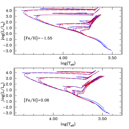
Figure 9: Comparison of our isochrones for [Fe/H]=0.06 and [Fe/H]=$-$1.55 (solid lines) with the older BaSTI isochrones for [Fe/H]=0.06 and [Fe/H]=$-$1.49 (dashed lines), and ages equal to 30 Myr, 100 Myr, 1 Gyr, 3 Gyr, 5 Gyr and 12 Gyr, respectively (see text for details).

The new isochrones have slightly hotter RGBs, and TO. The core He-burning sequences are brighter for ages below 1 Gyr, and the HRD blue-loops are generally more extended. Figure 10 enlarges the core He-burning portion of the isochrones for ages between 1 and 12 Gyr. The new isochrones have slightly fainter luminosities (by a few hundredth dex) during core He-burning at these ages –mainly because of the new electron conduction opacities– and slightly hotter effective temperatures, as for the RGB. At 12 Gyr and [Fe/H]$-$1.55 the new isochrones show a cooler He-burning phase, because of the lower of $\eta$ used in the new calculations.

The main reason for the differences between these new BaSTI computations and the previous ones is the updated solar metal distribution and associated lower $Z$ at a given [Fe/H]. However, the lower luminosity of the core He-burining phase at old ages is driven by the updated electron conduction opacities employed in these new calculations.

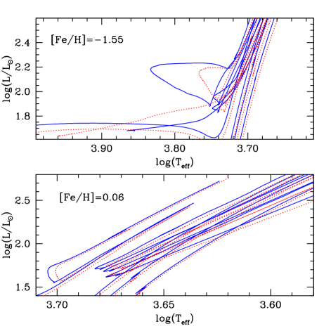
Figure 10: As Fig. 9 but showing the core He-burning region for ages between 1 and 12 Gyr. The older BaSTI isochrones are displayed as dotted lines.

Table 7: Main differences amongst the physics inputs and solar metal mixture adopted in our calculations and the independent calculations discussed in this section. The symbol ‘—’denotes the same treatment as in our calculations.

Code	EOS	Reaction rates	Opacity	Solar mix
Tognelli et al. (2011)	OPAL	—	—	Asplund et al. (2005)
(pre-MS)	(Rogers & Nayfonov, 2002b)
Siess et al. (2000)	Own calculations	Caughlan & Fowler (1988)	low-T opacities (Alexander & Ferguson, 1994)	Grevesse & Noels (1993)
(pre-MS)			electron conduction (Iben, 1975)
PARSEC	—	JINA REACLIB	low-T opacities (Marigo & Aringer, 2009)	–
		(Cyburt et al., 2010)	electron conduction (Itoh et al., 2008)
MESA	Saumon et al. (1995b)	JINA REACLIB	—	Asplund et al. (2009)
	Rogers & Nayfonov (2002b)
	MacDonald & Mullan (2012)

Table 8: As Table 7, but for the differences in the treatment of convective mixing, mass loss, mixing length and outer boundary conditions.

Code	Mixing	Reimers $\eta$ and $\alpha_{\rm ML}$	Bound. cond.	Diffusion
Tognelli et al. (2011)	—	$\eta$=0.0	theoretical
(pre-MS)		$\alpha_{\rm ML}$=1.9	model atmospheres
Siess et al. (2000)	—	$\eta$=0.0	theoretical	—
(pre-MS)		$\alpha_{\rm ML}$=1.605	model atmospheres
PARSEC	proportional mean free path across	$\eta$=0.2	gray $T(\tau)$ plus calibrated	off when conv. envelope
	border all conv. regions (Bressan et al., 1981)	$\alpha_{\rm ML}$=1.74	$T(\tau)$ for VLM models	mass below a threshold
MESA	Ledoux criterion, diffusive mixing	$\eta$=0.1 (RGB)	theoretical	moderated with
	diffusive overshooting/semiconv.	$\eta$=0.2 (AGB)	model atmospheres	diffusive mixing
		$\alpha_{\rm ML}$=1.82
		(Henyey et al., 1965) formalism

5.1 Pre-MS isochrones

We have compared our new isochrones with independent calculations, considering separately pre-MS isochrones for low- and very low-mass stars, that with our grid of models can be calculated for a minimum age of just 4 Myr, whereas complete isochrones reaching the AGB phase or C-ignition start from an age of 20 Myr.

The pre-MS isochrones have been compared to results from the extensive database by Tognelli et al. (2011), and the ‘classic’ models by Siess et al. (2000), as shown in Fig. 11. These latter two calculations differ from ours concerning some physics inputs. In particular, Tognelli et al. (2011) isochrones have been calculated adopting a different EOS and boundary conditions, whilst Siess et al. (2000) isochrones have been computed with different low-temperature radiative opacities, EOS, boundary conditions, and the initial deuterium abundance is about half the value used in our calculations. The reference solar metal mixture is different for each of the three sets of isochrones shown in the figure. The minimum evolving mass along the isochrones is equal to 0.1$M_{\odot}$ for our and Siess et al. (2000) calculations, while it is equal to 0.2$M_{\odot}$ for Tognelli et al. (2011) models.

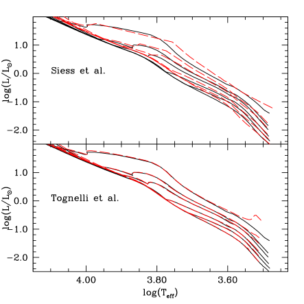
Figure 11: Comparison of our pre-MS isochrones (solid lines) with Siess et al. (2000) and Tognelli et al. (2011) results (dashed lines in the top and bottom panel, respectively) for a metallicity around solar and ages equal to 4, 10, 15, 30, 50, and 100 Myr, respectively (see text for details).

For the comparison we have selected Tognelli et al. (2011) calculations (that at fixed $Z$ allow for various choices of $Y$, the deuterium mass fraction $X_{D}$ and mixing length) for $Z$=0.0175, $Y$=0.265 $X_{D}=4\ 10^{-5}$, $\alpha_{\rm ML}$=1.9 –very close to our initial solar chemical composition, the adopted initial deuterium mass fraction and solar calibrated mixing length– and the $Z$=0.02 Siess et al. (2000) isochrones. We have considered ages equal to 4, 10, 15, 30, 50, and 100 Myr, respectively. The upper age limit is fixed by the largest age available for Tognelli et al. (2011) calculations.

The agreement between our $Z$=0.0172 ([Fe/H]=0.06) and Tognelli et al. (2011) isochrones is remarkable. They are almost indistinguishable, appreciable differences appearing only for the lowest masses in common and the two youngest ages, where Tognelli et al. (2011) isochrones are more luminous than ours at a given $T_{eff}$. Differences with respect to Siess et al. (2000) calculations are larger and more systematic, their isochrones being almost always brighter at fixed $T_{eff}$ for stellar masses between $\sim$2.0-2.5 $M_{\odot}$ and $\sim$0.4$M_{\odot}$.

5.2 MS and post-MS isochrones

Our complete isochrones have been compared with results from the recent PARSEC and MIST isochrones. We considered the non-rotating MIST isochrones, and the PARSEC isochrones with VLM stellar models calculated with the ‘calibrated’ boundary conditions, as described in Chen et al. (2014).

We considered our isochrones including convective core overshooting during the MS and atomic diffusion (the reference set a) described in Table 3), for both effects are included in the MIST and PARSEC isochrones, although with varying implementations. Compared to our models, the non-rotating MIST isochrones have been calculated with different implementations of convective mixing (and include thermohaline mixing during the RGB), as well as different choices for the solar metal distribution, EOS, reaction rates, boundary conditions, mixing length theory formalism, and a lower value of the Reimers $\eta$ parameter. Radiative levitation is neglected, and the efficiency of atomic diffusion during the MS is moderated by including a competing turbulent diffusive coefficient (see Choi et al., 2016, for details).

The PARSEC calculations have employed, compared to our new models, different choices for the low-temperature radiative opacities, electron conduction opacities, reaction rates, implementation of overshooting, boundary conditions, and a lower value of the Reimers parameter $\eta$. Atomic diffusion without radiative levitation is included, but switched off when the mass size of the outer convective region decreases below a given threshold (see Bressan et al., 2012, for details).

Figures 12 and 13 show selected isochrones for 30 Myr, 100 Myr, 1 Gyr, 3 Gyr, 5 Gyr and 12 Gyr, [Fe/H]=0.06 and [Fe/H]=$-$1.55, respectively. They are shown together with PARSEC isochrones for the same ages, [Fe/H]=0.07 and $-$1.59, and MIST isochrones for the same ages and [Fe/H] of our isochrones .

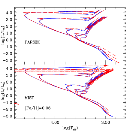
Figure 12: Comparison of our complete isochrones for [Fe/H]=0.06 (solid lines) with PARSEC and MIST results (dashed lines in the top and bottom panel, respectively) and ages equal to 30 Myr, 100 Myr, 1 Gyr, 3 Gyr, 5 Gyr and 12 Gyr, respectively (see text for details).

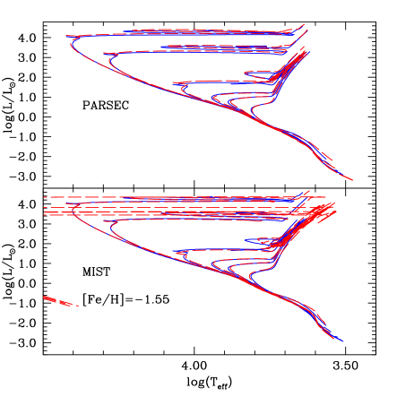
Figure 13: As Fig. 12 but for [Fe/H]=$-$1.55 (see text for details).

The comparison with PARSEC isochrones displays a remarkable general agreement especially at the lower [Fe/H], whereas at the higher metallicity the lower masses (that are still evolving along the pre-MS phase in the youngest two isochrones) are systematically discrepant compared to our models. The TO luminosities are only slightly different, especially at the three lowest ages, where the effect of different core overshooting prescription may play a role. The core He-burning phase is slightly over-luminous compared to our models, RGBs are slightly cooler compared to our [Fe/H]=0.06 isochrones, and slightly hotter compared to the [Fe/H]=$-$1.55 ones. Figures 14 and 15 enlarge the core He-burning portion of the isochrones for ages between 1 and 12 Gyr. The RGB of PARSEC isochrones is cooler by less than 100 K compared to our models for [Fe/H]=0.06, and hotter by less than 100 K at the lower metallicity. The luminosity of the He-burning phase is only slightly larger (by a few hundredth dex) at both metallicities. Notice that at 12 Gyr the start of quiescent core He-burning in our isochrones is at a hotter $T_{eff}$ than PARSEC results, due to our choice of a larger $\eta$ Reimers parameter.

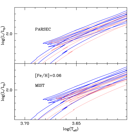
Figure 14: As Fig. 12 but showing the core He-burning region for ages between 1 and 12 Gyr. MIST and PARSEC isochrones are displayed as dotted lines.

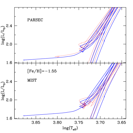
Figure 15: As Fig. 14 but for [Fe/H]=$-$1.55.

The comparison with MIST isochrones yields similar results. There is an overall good agreement for the MS, TO, subgiant-branch (SGB) phases, and also in the regime of the lowest masses, still evolving along the pre-MS at the youngest ages. The He-burning phase of MIST isochrones is generally over-luminous, RGBs systematically redder at [Fe/H]=0.06, and with a different slope at [Fe/H]=$-$1.55. Figures 14 and 15 show RGBs over 100 K cooler than our models at [Fe/H]=0.06, and slightly larger core He-burning luminosities, like in the comparison with PARSEC. Also in comparison with MIST isochrones, at 12 Gyr the start of quiescent core He-burning in our isochrones is at a hotter $T_{eff}$, again due to our choice of a larger $\eta$ Reimers parameter.

6 Comparisons with data

In this section we present results of some tests, performed to assess the general consistency of our new models and isochrones with constraints coming from eclipsing binary analyses, stars with asteroseismic mass determinations, and star clusters. The isochrones used in these comparisons include convective core overshooting during the MS for the appropriate age range and neglect atomic diffusion during the MS (set b) of models described in Table 3), if not otherwise specified.

6.1 Binaries

We first consider masses and radii for pre-MS detached eclipsing binary (DEB) systems compiled by Stassun et al. (2014) and Simon & Toraskar (2017), covering a mass range between 0.2 and 4.0$M_{\odot}$. We assume an initial [Fe/H]=0.06 (overall consistent with the few available spectroscopic estimates, see Stassun et al., 2014), and consider a minimum age of 4 Myr, the lowest possible value with our model grid. We do not aim to find a best-fit solution for all the systems, just at least one isochrone that matches simultaneously mass and radius of both components for each system within the errors, to denote a general consistency between models and observations.

This test is relevant for the general adequacy of both boundary conditions and $\alpha_{\rm ML}$ value employed in the calculations, given the extreme sensitivity of pre-MS tracks to the combination of these two inputs. It is however worth noticing that the lack of model-independent age estimates prevent this type of tests from providing very stringent constraints on the models.

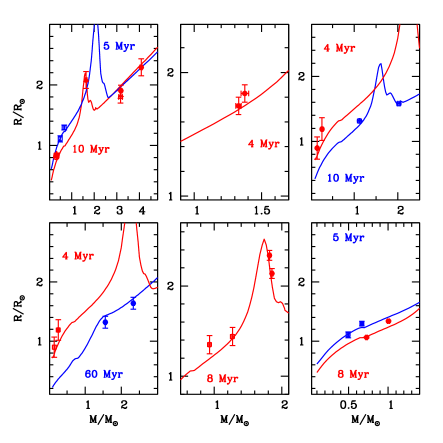
Figure 16: Comparison in the MR diagram between our pre-MS isochrones and a sample of pre-MS DEB systems (see text for details). Notice the local maximum of the radius displayed by the 4, 5, 8, and 10 Myr isochrones, corresponding to C and N abundances attaining their equilibrium abundances.

We found 13 systems in the age range covered by our pre-MS isochrones, displayed in a mass-radius (MR) diagram in Fig. 16. In case of all these systems, our isochrones can match both components within the quoted 1$\sigma$ error bars with a single age value, varying between 5 and 60 Myr among the whole sample of DEBs.

The next test involves low-mass MS models. It has been recognized since some time the existence of a disagreement between theoretical and observational MR relationships for low-mass stars, with model radii typically 10-20% smaller than observations for a fixed mass, (see, e.g., Torres et al., 2010, for a review). Here we examine first the level of agreement between the observed and theoretical MS low-mass MR relationship, by comparing our grid of models with data from DEB systems that host components with M$<0.8~{}M_{\odot}$, as compiled by Feiden & Chaboyer (2012). This compilation includes systems with quoted random uncertainties in both mass and radius below 3%. As for the pre-MS case, the requirement for the models is that they are able to match the position of both system components in the MR diagram for a single value of the age.

We assume that all DEBs have metallicity around solar (see also Feiden & Chaboyer, 2012, for spectroscopic metallicity estimates for a few of the systems in their compilation) and split the sample into two subsamples. The first one is made of systems with both components essentially on the ZAMS, displayed in Fig.17, together with isochrones of ages equal to 1 Gyr and 12 Gyr respectively, and [Fe/H]=0.06. We also show a 12 Gyr isochrone for [Fe/H]=$-$0.40, to highlight the insensitivity of the theoretical MR relationship to metallicity, when the mass is below $\sim$0.7 $M_{\odot}$.

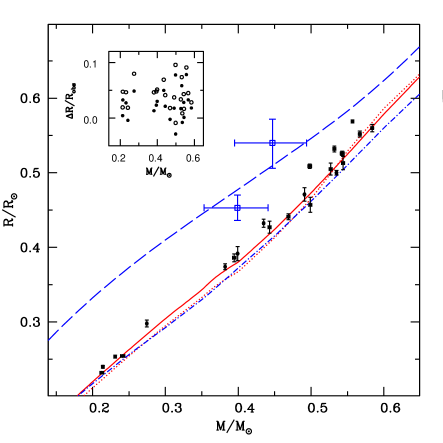
Figure 17: Comparison in the MR diagram between our 1 Gyr (dashed dotted line) and 12 Gyr (solid line) [Fe/H]=0.06 isochrones, and a subsample of Feiden & Chaboyer (2012) DEB systems whose components are found to be evolving on the ZAMS. The dotted line denotes a 12 Gyr old [Fe/H]=$-$0.40 isochrone, to show the almost negligible effect of metallicity variations when the mass is below $\sim$0.7$M_{\odot}$. Open squares denote the components of the system KELT J041621-62004. The dashed line displays a 50 Myr, [Fe/H]=0.06 pre-MS isochrone. The inset shows the run of the relative radius differences (observations-theory) $\Delta R/R_{\rm obs}$ with the mass of the systems’ components (bar the system KELT J041621-62004) for an age of 1 Gyr (open circles) and 12 Gyr (filled circles – see text for details).

Figure 18: As Fig. 17 but for Feiden & Chaboyer (2012) DEB systems with at least one component evolved off the ZAMS.

Isochrones appear to match reasonably well all systems, without a clear major systematic discrepancy in radius at fixed mass. The effect of age is very small for this mass range. If we denote with $\Delta R$ the difference $R_{\rm obs}-R_{\rm theory}$ between observed and predicted radius for an object with observed mass $M$, we find an average $\Delta R/R_{\rm obs}$=0.02$\pm$0.03 assuming an age of 12 Gyr for all systems, and an average $\Delta R/R_{\rm obs}$=0.04$\pm$0.03 for an age of 1 Gyr (see inset of Fig. 17). These average differences are consistent with typical systematic errors on empirical radius estimates –of the order of 2-3%– as determined by Windmiller et al. (2010) in their reanalysis of the DEB system Gu Boo.

The second subsample (see Fig.18) includes systems with one or both components evolved off the ZAMS. We impose an upper limit of 13.5 Gyr to their ages, to match the cosmological constraint. The major discrepancy here is for UV Psc, whereby one component is matched by the 9 Gyr isochrone, whereas the less massive one appears older than 13.5 Gyr. A minor discrepancy affects also IM Vir, with the lower mass component appearing slightly older than the companion.

On the whole there is no major systematic discrepancy between models and observed MR relationships, although there are clear mismatches for a few cases, as found also by Feiden & Chaboyer (2012) analysis. Another example of mismatch is the M-dwarf system (both components with masses around $0.4~{}M_{\odot}$) KELT J041621-620046 studied very recently by Lubin et al. (2017), and shown in Fig.17. Our isochrones give radii systematically lower than observed for both components (as all other models employed by Lubin et al., 2017) by $\sim$20%. The commonly accepted explanation for these mismatches (see, e.g., Feiden & Chaboyer, 2012; Lubin et al., 2017, and references therein) involves effects of large-scale magnetic fields that suppress convective motions, and increase the total surface coverage of starspots. This causes a reduction in the total energy flux across a given surface within the star, forcing the stellar radius to inflate and ensure flux conservation. For the sake of comparison we also show in Fig.17 a 50 Myr, [Fe/H]=0.06 pre-MS isochrone that would match within the error bars the position of KELT J041621-620046 components in the MR diagram, in case these objects were actually pre-MS stars.

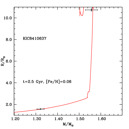
Figure 19: As Fig. 17 but for the components of the KIC 8410637 system (see text for details).

The next comparison involves the DEB system KIC 8410637, studied by Frandsen et al. (2013). It contains a MS and a RGB star, and is another good test for the calibration of convection in the models. Figure 19 compares observations and isochrones in the MR diagram. When considering isochrones for [Fe/H]=0.06, consistent with the spectroscopic estimate by Frandsen et al. (2013), we find that an age of 2.5 Gyr matches very well the position of the two components (a similar result was found by Frandsen et al., 2013, using PARSEC isochrones).

The last DEB systems compared to our models are four objects from Claret & Torres (2017) compilation. Their spectroscopic metallicity is consistent within errors with [Fe/H]=$-$0.40; the mass of the various components ranges between $\sim$1.4 and $\sim$4.2 $M_{\odot}$, and they are evolving along either the RGB or core He-burning phase. Figure 20 compares their MR diagrams with theoretical isochrones for [Fe/H]=$-$0.40, that are able to match simultaneously both components (within their mass and radius error bars) in all four systems for the labelled ages, with our choices of MS core overshooting efficiency and mixing length.

Figure 20: As Fig. 17 but for the components of –moving clockwise from the top left panel– OGLE-LMC-ECL-06575, OGLE-LMC-ECL-09660, OGLE-LMC-ECL-15260 and OGLE-LMC-ECL-03160 systems (see text for details).

Finally, we compare the mass-luminosity relationship predicted by our low-mass models in the $V$ and $K$ bands, with the data presented by Delfosse et al. (2000), based mainly on visual and interferometric pairs. We display in Fig. 21 the observational data together with three isochrones with [Fe/H]=0.06 and ages equal to 300 Myr, 1 Gyr and 10 Gyr respectively (solid lines), plus two 10 Gyr isochrones with [Fe/H]=$-$0.40 and [Fe/H]=0.45 respectively (dashed lines).

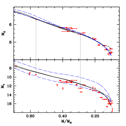
Figure 21: Comparison of theoretical and observed mass-luminosity relationships in the $V$ and $K$ bands for a sample of low-mass stars from Delfosse et al. (2000). Filled symbols with error bars display the data, whilst solid lines correspond to three isochrones with [Fe/H]=0.06 and ages equal to 300 Myr, 1 Gyr and 10 Gyr respectively. The dashed lines show 10 Gyr isochrones with [Fe/H]=$-$0.40 (brighter at fixed mass compared to the [Fe/H]=0.06 isochrones) and [Fe/H]=0.45, respectively. Dotted lines highlight two objects that are inconsistent with the models in the $V$-band, but fully consistent in the $K$-band (see text for details).

First of all, as also noted by Delfosse et al. (2000), the $V$-band data show a large dispersion at fixed $M$, with models matching a sort of upper envelope of the data. The $K$-band data are much tighter, and in very good general agreement with the [Fe/H]=0.06 models, even though the sample is smaller than for the $V$-band. It is interesting to consider the two objects highlighted by the dotted lines. They have estimates of both $V$ and $K$ absolute magnitudes; in the $K$-band the agreement with theory for [Fe/H]=0.06 (or higher) is essentially perfect, whereas in the $V$-band the data are clearly under-luminous compared to the models. The fact that the $V$-band diagram is much more sensitive to the exact metallicity of the sample (as shown by the dashed lines in the figure) suggests that [Fe/H] may play a role in explaining this dispersion. The [Fe/H]=0.45 isochrone is under-luminous at fixed mass compared to the [Fe/H]=0.06 one, but still cannot explain the full dispersion of the data.

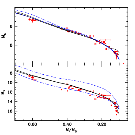
Figure 22: As Fig. 21 but for observed mass-luminosity relationships from Benedict et al. (2016) (see text for details).

Figure 22 displays a similar comparison with the more recent mass-luminosity empirical data by Benedict et al. (2016). Also in this case the dispersion in the $V$-band is larger than in the $K$-band. In the $K$-band (weakly sensitive to chemical composition) the agreement with theory is again generally quite good, apart from the cluster of objects with mass around 0.6$M_{\odot}$, that appear somewhat underluminous with respect to the models, irrespective of the adopted metallicity between [Fe/H]=$-$0.4 and 0.45.

6.2 Stars with asteroseismic mass determinations

A recent study by Tayar et al. (2017) has provided a sample of over 3000 RGB stars with $T_{eff}$, mass (determined from asteroseismic scaling relations), surface gravity, [Fe/H] and $\alpha$-enhancement ([$\alpha$/Fe]) determinations from the updated APOGEE-Kepler catalog. These stars cover a log(g) range between $\sim$3.3 and 1.1 (in cgs units), and $T_{eff}$ between $\sim$5200 and 3900 K, with the bulk of the stars having [Fe/H] between $\sim-$0.7 and $\sim$ +0.4 dex, and a maximum $\alpha$-enhancement typically around 0.25 dex. This sample allows to compare empirically determined $T_{eff}$ values (calibrated on the González Hernández & Bonifacio, 2009, temperature scale) with theoretical models of the appropriate chemical composition, that are very sensitive to the treatment of the superadiabatic layers, hence the calibration of $\alpha_{\rm ML}$.

In our comparison we have considered only stars with [$\alpha$/Fe]$<$0.07 (this upper limit corresponds to approximately 3-5 times the quoted 1$\sigma$ error on [$\alpha$/Fe]), but an upper limit closer to zero does not change our results. We have calculated differences $\Delta T\equiv T_{obs}-T_{models}$ between observed and theoretical $T_{eff}$ for each individual star, by interpolating linearly in mass, [Fe/H] and log(g) amongst our models, to determine the corresponding theoretical $T_{eff}$. The $\Delta T$ values for [Fe/H] larger than $\sim-$0.7 dex have been collected in ten [Fe/H] bins with total width of 0.10 dex, apart from the most metal poor one, that has a width of 0.20 dex, due to the smaller number of stars populating that metallicity range. We have then performed a linear fit to the mean $\Delta T$ values of each bin, and derived a slope equal to 14 $\pm$ 11 K/dex, statistically different from zero at much less than 2$\sigma$ (see Fig. 23). The average $\Delta T$ is equal to just $-$14 K, with a 1$\sigma$ dispersion of 34 K. This small offset between models and observations is well within the error on the González Hernández & Bonifacio (2009) $T_{eff}$ calibration (the quoted average error on their RGB $T_{eff}$ scale is $\leq$76 K).

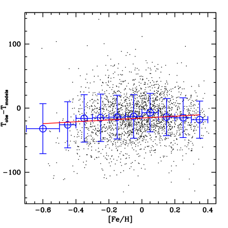
Figure 23: $\Delta T$ as a function of [Fe/H] (dots) for RGB stars with asteroseismic mass determinations from Tayar et al. (2017), and ${\rm[\alpha/Fe]<0.07}$. Open circles with error bars denote the mean values of $\Delta T$ in specific metallicity bins, while the solid line displays a linear fit to the binned data. Vertical error bars denote the 1$\sigma$ dispersion of around the mean values of $\Delta T$ in each bin, whereas the horizontal error bars denote the width of the [Fe/H] bins.

6.3 Star clusters

The following comparisons with CMDs of a sample of Galactic open clusters and one globular cluster (with solar scaled initial metal distribution) provide additional tests of the reliability of our evolutionary tracks/isochrones plus the adopted bolometric corrections. In all these comparisons we have included the effect of extinction according to the standard Cardelli et al. (1989) reddening law, with $R_{V}\equiv A_{V}/E(B-V)$=3.1.

Figure 24 displays $BVJHK_{s}$ CMDs ($JHK_{s}$ from 2MASS photometry) for Hyades members taken from Röser et al. (2011) and Kopytova et al. (2016), that reach the VLM star regime, down to $\sim$0.2$M_{\odot}$. We have calculated absolute magnitudes by applying the secular parallaxes determined by Röser et al. (2011). The average parallax of these objects is in agreement with the average value of 103 probable members of the Hyades from the $Gaia$ data release 1, as given by Gaia Collaboration et al. (2017), within the quoted errors. We display also color and absolute magnitude error bars (the error bars on the absolute magnitudes account also for the contribution of the parallax errors) given that color errors often are non negligible along the MS.

The cluster CMDs are compared with our $t$=600 and 800 Myr, [Fe/H]=0.06 isochrones – close to spectroscopic estimates [Fe/H]=0.14$\pm$0.05 (Cayrel de Strobel et al., 1997) and [Fe/H]=0.10$\pm$0.01 (Taylor & Joner, 2005) – assuming $E(B-V)$=0, consistent with the results by Taylor (2006). The age range bracketed by these two isochrones is representative of the range of ages estimated for this cluster, as recently debated in the literature (see, e.g. Perryman et al., 1998; Brandt & Huang, 2015, and references therein)].

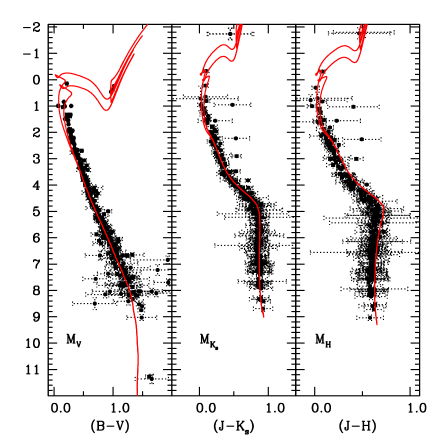
Figure 24: Comparison between our 600 and 800 Myr, [Fe/H]=0.06 isochrones, and three Hyades CMDs, corrected for the secular parallaxes determined by Röser et al. (2011) –see text for details.

The theoretical isochrones follow well the observed MS down to the faintest limit, apart from the $JH$ diagram, that shows a systematic offset due to the $H$-band bolometric corrections, although models are still consistent with the data within the associated error bars.

Optical CMDs of NGC 2420 (Anthony-Twarog et al., 1990) and M 67 (Sandquist, 2004) are shown in Fig. 25, compared to isochrones with $t$=2.5 Gyr and [Fe/H]=$-$0.40 in case of NGC 2420, $t$=4 Gyr and [Fe/H]=0.06 for M 67, respectively. These metallicities are consistent with [Fe/H]=$-$0.44$\pm$0.06 (NGC2420) and [Fe/H]=0.02$\pm$0.06 (M67) quoted by Gratton (2000). The isochrones have been shifted to account for distance moduli and reddenings $(m-M)_{0}$=11.95, $E(B-V)$=0.06 for NGC 2420, and $(m-M)_{0}$=9.64, $E(B-V)$=0.02 for M 67. These pairs of values are consistent with the reddening estimates by Twarog et al. (1997) and MS-fitting distance moduli (using dwarfs with accurate Hipparcos parallaxes) by Percival & Salaris (2003), within their error bars.

The values of the mass evolving at the TO for NGC 2420 and M 67 isochrones are $\sim$1.3$M_{\odot}$ and $\sim$1.2$M_{\odot}$ respectively, in the mass range where the size of the overshooting region is decreased down to zero from the standard value of 0.2$H_{p}$. The shape of the TO region –sensitive to the extent of the overshooting region– is well traced by the isochrones for both clusters, lending some support to our prescription for the reduction of size of the overshooting region with mass.

One can notice also how, in addition to the MS (apart from the faintest end of NGC 2420 MS), also RGB, SGB and red clump sequences are nicely matched by the isochrones.

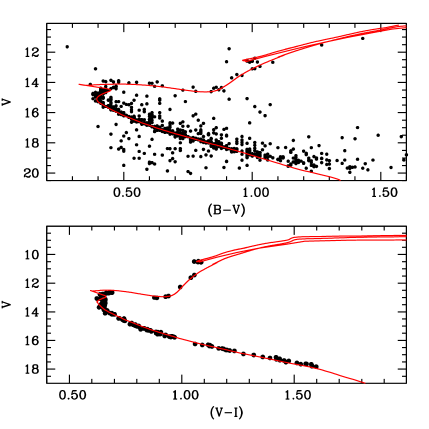
Figure 25: Optical CMDs for NGC 2420 (top panel) and M 67 (bottom panel). Our isochrones with [Fe/H]$-$0.40, $t$=2.5 Gyr, $(m-M)_{0}$=11.95, $E(B-V)$=0.06 (top panel) and [Fe/H]=0.06, $t$=4 Gyr, $(m-M)_{0}$=9.64, $E(B-V)$=0.02 (bottom panel) are also shown (see text for details).

The next object compared to our isochrones is the old and super metal rich open cluster NGC 6791. At the super-solar metallicity of this object, bolometric corrections are bound to be more uncertain, because inaccuracies in atomic and molecular opacity data entering the model spectra calculations are greatly enhanced in this metallicity regime.

For this cluster we take advantage of the analysis by Brogaard et al. (2011) and Brogaard et al. (2012) of two DEB systems, that provide estimates of $E(B-V)$=0.16$\pm$0.025, $(m-M)_{V}$=13.51$\pm$0.06, [Fe/H]=+0.29$\pm$0.03(random)$\pm$0.07(systematic), this latter value in agreement, within the errors, with spectroscopic estimates by Origlia et al. (2006) and Carraro et al. (2006), but lower than [Fe/H]=+0.47$\pm$0.04 determined by Gratton et al. (2006).

Figure 26 displays the MR diagram for the four components (the primary component of V20 is in the TO region of the CMD, the other components are increasingly fainter MS stars) of these two DEB systems (named V18 and V20 in Brogaard et al., 2011) including the 1$\sigma$ and 3$\sigma$ error bars, together with two theoretical isochrones for [Fe/H]=0.30, with and without the inclusion of atomic diffusion, and ages of 8.5 Gyr and 9.0 Gyr, respectively.

As for the isochrones discussed by Brogaard et al. (2012) it is not possible to match perfectly the MR diagram of these EBs with theoretical isochrones. Those shown in Fig. 26 represent the best compromise to match the data for the four DEB components, within their errors.

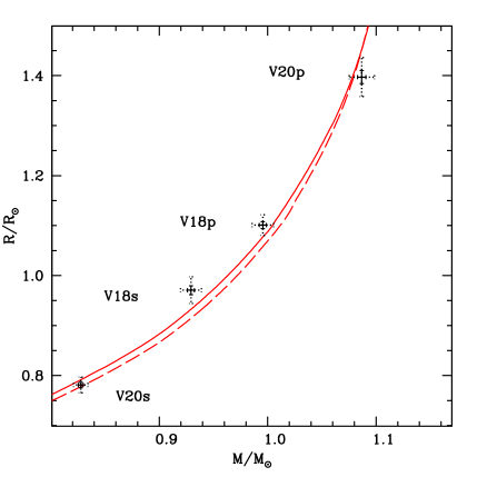
Figure 26: Comparison in the MR diagram between the primary and secondary components of the DEB systems V18 and V20 in NGC6791, and our [Fe/H]=0.30 isochrones with $t$=8.5 Gyr including atomic diffusion (solid line), and $t$=9.0 Gyr without atomic diffusion (dashed line).

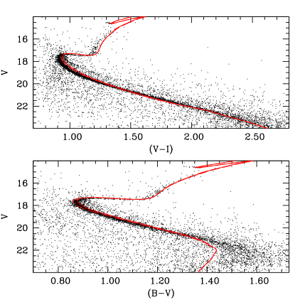
Figure 27: $BVI$ CMDs for NGC 6791, compared to the same isochrones of Fig. 26. The isochrones have been shifted in magnitude and colors by $(m-M)_{V}$=13.52 (isochrone with diffusion, shown as a solid line) and $(m-M)_{V}$=13.54 (isochrone without diffusion, shown as a dashed line), and $E(B-V)$=0.16 (see text for details).

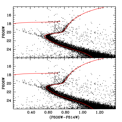
Figure 28: Optical $HST$/ACS CMD for Rup 106, compared to our ZAHB sequences and isochrones with [Fe/H]=$-$1.55, $t$=12.5 Gyr, $(m-M)_{0}$=16.69, $E(B-V)$=0.18 and no atomic diffusion (top panel), and $t$=11.5 Gyr $(m-M)_{0}$=16.66, $E(B-V)$=0.18, including atomic diffusion (lower panel – see text for details).

Figure 27 places the same isochrones of the DEBs comparison in optical $BVI$ CMDs, together witj the cluster photometry, corrected for differential reddening, by Brogaard et al. (2012). We have displayed only stars with good quality photometry, i.e. we have considered only objects with photometric reduction yielding a $sharp$ index between -0.4 and +0.4, and a $chi$ index between 0.9 and 1.2. The isochrones have been shifted in colour for a reddening $E(B-V)$=0.16, and vertically for $(m-M)_{V}$=13.52 (the isochrone with diffusion) and $(m-M)_{V}$=13.54 (the isochrone without diffusion) respectively. These distance moduli, both consistent with the result from the DEB analyses, allow to match the $V$-band magnitude of the observed red clump stars with the core-He-burning portion of the isochrones. The overall comparison is better in the $BV$ CMD, where the RGB location and slope is reasonably reproduced, as well as the TO-SGB-upper MS sequence. The TO region is matched better by the isochrone including atomic diffusion. In $VI$ the match is overall worse. The RGB of the isochrones is redder than observed, the TO-SGB region is less well reproduced than in $BV$, although the lower MS is better matched.

As a last object, we have considered the low-mass (total actual mass lower than $10^{5}M_{\odot}$, see Villanova et al., 2013) outer halo Galactic globular cluster Rup 106, whose stars display a solar scaled metal distribution, without the O-Na and C-N abundance anticorrelations common in other Galactic globular clusters (Villanova et al., 2013). Figure 28 shows the cluster optical CMD in the $HST$/ACS camera photometric system (Dotter et al., 2011), together with isochrones for [Fe/H]=$-$1.55 –close to the mean value [Fe/H]=$-$1.47$\pm$0.02 determined spectroscopically by Villanova et al. (2013) – $t$=12.5 Gyr (without atomic diffusion) and $t$=11.5 Gyr (including atomic diffusion), and ZAHB sequences (obtained from models with and without diffusion, respectively) for the same metallicity. A reddening $E(B-V)$=0.18 and distance moduli $(m-M)_{0}$=16.66 (for isochrones and ZAHB models with diffusion) and $(m-M)_{0}$=16.69 (for isochrones and ZAHB models without diffusion) have been applied to the models. The distance moduli have been fixed by matching the theoretical ZAHB sequences to the lower envelope of the observed HB.

The isochrones follow well the observed CMD. The TO region is better matched by the isochrone including atomic diffusion. Increasing the age of the isochrone without diffusion to make its TO redder does not improve the match with observations, because the model SGB would become fainter than the observed one.

7 Conclusions

In this paper we have presented a comprehensive overview of the updated BaSTI models, discussing the change in physics inputs compared to the previous BaSTI calculations, including comparisons with recent independent stellar model and isochrone databases, and a host of observational tests. Improving upon the previous BaSTI release, this new library increases significantly the number of available metallicities, includes also the VLM regime, accounts consistently for the pre-MS evolution in the isochrone calculations, and provides also asteroseismic properties of the models.

Our new models/isochrones are able to match several sets of independent observational constraints that involve pre-MS stars and objects in more advanced evolutionary phases, either single, in DEBs or in star clusters. We believe that this updated BaSTI release will be an important tool to investigate field and cluster, Galactic and extragalaxy stellar populations.

We make publicly available the whole database of models and isochrones through a dedicated Web site at the following URL address: http://basti-iac.oa-abruzzo.inaf.it. Here we provide tables of stellar evolutionary tracks and asteroseismic properties of our grid of stellar evolution calculations plus isochrones, in several photometric systems. We can also provide, upon request, additional calculations and both evolutionary and asteroseismic outputs, for stellar masses not in our standard grids.

In the near future we will set up a Web interface to enable interpolations in metallicity within the available track and isochrone grids, as well as the calculations of isochrones and luminosity functions for any specified age.

The next paper of this series will present $\alpha-$enhanced and $\alpha-$depleted models and isochrones, particularly suited to study stellar populations in globular clusters and dwarf galaxies.

References

- Alexander & Ferguson (1994) Alexander, D. R., & Ferguson, J. W. 1994, ApJ, 437, 879
- Allard et al. (1997) Allard, F., Hauschildt, P. H., Alexander, D. R., & Starrfield, S. 1997, ARA&A, 35, 137
- Allard et al. (2012) Allard, F., Homeier, D., & Freytag, B. 2012, Philosophical Transactions of the Royal Society of London Series A, 370, 2765
- Anders & Grevesse (1989) Anders, E., & Grevesse, N. 1989, Geochim. Cosmochim. Acta, 53, 197
- Andrássy & Spruit (2013) Andrássy, R., & Spruit, H. C. 2013, A&A, 559, A122
- Andrássy & Spruit (2015) —. 2015, A&A, 578, A106
- Angulo et al. (1999) Angulo, C., Arnould, M., Rayet, M., et al. 1999, Nuclear Physics A, 656, 3
- Anthony-Twarog et al. (1990) Anthony-Twarog, B. J., Twarog, B. A., Kaluzny, J., & Shara, M. M. 1990, AJ, 99, 1504
- Asplund et al. (2005) Asplund, M., Grevesse, N., & Sauval, A. J. 2005, in Astronomical Society of the Pacific Conference Series, Vol. 336, Cosmic Abundances as Records of Stellar Evolution and Nucleosynthesis, ed. T. G. Barnes, III & F. N. Bash, 25
- Asplund et al. (2009) Asplund, M., Grevesse, N., Sauval, A. J., & Scott, P. 2009, ARA&A, 47, 481
- Baglin et al. (2009) Baglin, A., Auvergne, M., Barge, P., et al. 2009, in IAU Symposium, Vol. 253, IAU Symposium, ed. F. Pont, D. Sasselov, & M. J. Holman, 71–81
- Bahcall et al. (1995) Bahcall, J. N., Pinsonneault, M. H., & Wasserburg, G. J. 1995, Reviews of Modern Physics, 67, 781
- Baraffe et al. (1995) Baraffe, I., Chabrier, G., Allard, F., & Hauschildt, P. H. 1995, ApJ, 446, L35
- Basu (1997) Basu, S. 1997, MNRAS, 288, 572
- Basu & Antia (2004) Basu, S., & Antia, H. M. 2004, ApJ, 606, L85
- Beck et al. (2011) Beck, P. G., Bedding, T. R., Mosser, B., et al. 2011, Science, 332, 205
- Bedding et al. (2011) Bedding, T. R., Mosser, B., Huber, D., et al. 2011, Nature, 471, 608
- Benedict et al. (2016) Benedict, G. F., Henry, T. J., Franz, O. G., et al. 2016, AJ, 152, 141
- Bergemann & Serenelli (2014) Bergemann, M., & Serenelli, A. 2014, Solar Abundance Problem, ed. E. Niemczura, B. Smalley, & W. Pych, 245–258
- Bessell et al. (2011) Bessell, M., Bloxham, G., Schmidt, B., et al. 2011, PASP, 123, 789
- Bessell (1990) Bessell, M. S. 1990, PASP, 102, 1181
- Bessell & Brett (1988) Bessell, M. S., & Brett, J. M. 1988, PASP, 100, 1134
- Bessell et al. (1998) Bessell, M. S., Castelli, F., & Plez, B. 1998, A&A, 333, 231
- Böhm-Vitense (1958) Böhm-Vitense, E. 1958, ZAp, 46, 108
- Brandt & Huang (2015) Brandt, T. D., & Huang, C. X. 2015, ApJ, 807, 24
- Bressan et al. (2012) Bressan, A., Marigo, P., Girardi, L., et al. 2012, MNRAS, 427, 127
- Bressan et al. (1981) Bressan, A. G., Chiosi, C., & Bertelli, G. 1981, A&A, 102, 25
- Brocato et al. (1998) Brocato, E., Cassisi, S., & Castellani, V. 1998, MNRAS, 295, 711
- Brogaard et al. (2011) Brogaard, K., Bruntt, H., Grundahl, F., et al. 2011, A&A, 525, A2
- Brogaard et al. (2012) Brogaard, K., VandenBerg, D. A., Bruntt, H., et al. 2012, A&A, 543, A106
- Caffau et al. (2011) Caffau, E., Ludwig, H.-G., Steffen, M., Freytag, B., & Bonifacio, P. 2011, Sol. Phys., 268, 255
- Caputo et al. (1989) Caputo, F., Chieffi, A., Tornambe, A., Castellani, V., & Pulone, L. 1989, ApJ, 340, 241
- Cardelli et al. (1989) Cardelli, J. A., Clayton, G. C., & Mathis, J. S. 1989, ApJ, 345, 245
- Carraro et al. (2006) Carraro, G., Villanova, S., Demarque, P., et al. 2006, ApJ, 643, 1151
- Casagrande et al. (2014) Casagrande, L., Silva Aguirre, V., Stello, D., et al. 2014, ApJ, 787, 110
- Casagrande et al. (2016) Casagrande, L., Silva Aguirre, V., Schlesinger, K. J., et al. 2016, Monthly Notices of the Royal Astronomical Society, 455, 987
- Cassisi et al. (2007) Cassisi, S., Potekhin, A. Y., Pietrinferni, A., Catelan, M., & Salaris, M. 2007, ApJ, 661, 1094
- Cassisi & Salaris (2013) Cassisi, S., & Salaris, M. 2013, Old Stellar Populations: How to Study the Fossil Record of Galaxy Formation
- Cassisi et al. (2003) Cassisi, S., Salaris, M., & Irwin, A. W. 2003, ApJ, 588, 862
- Castellani et al. (1985) Castellani, V., Chieffi, A., Tornambe, A., & Pulone, L. 1985, ApJ, 296, 204
- Castelli (2005) Castelli, F. 2005, Memorie della Societa Astronomica Italiana Supplementi, 8, 34
- Castelli & Kurucz (2004) Castelli, F., & Kurucz, R. L. 2004, ArXiv Astrophysics e-prints, astro-ph/0405087
- Caughlan & Fowler (1988) Caughlan, G. R., & Fowler, W. A. 1988, Atomic Data and Nuclear Data Tables, 40, 283
- Cayrel de Strobel et al. (1997) Cayrel de Strobel, G., Crifo, F., & Lebreton, Y. 1997, in ESA Special Publication, Vol. 402, Hipparcos - Venice ’97, ed. R. M. Bonnet, E. Høg, P. L. Bernacca, L. Emiliani, A. Blaauw, C. Turon, J. Kovalevsky, L. Lindegren, H. Hassan, M. Bouffard, B. Strim, D. Heger, M. A. C. Perryman, & L. Woltjer, 687–688
- Chabrier & Baraffe (2000) Chabrier, G., & Baraffe, I. 2000, ARA&A, 38, 337
- Chaplin et al. (2011) Chaplin, W. J., Kjeldsen, H., Christensen-Dalsgaard, J., et al. 2011, Science, 332, 213
- Chaplin et al. (2015) Chaplin, W. J., Lund, M. N., Handberg, R., et al. 2015, PASP, 127, 1038
- Chen et al. (2014) Chen, Y., Girardi, L., Bressan, A., et al. 2014, MNRAS, 444, 2525
- Choi et al. (2016) Choi, J., Dotter, A., Conroy, C., et al. 2016, ApJ, 823, 102
- Christensen-Dalsgaard (2008) Christensen-Dalsgaard, J. 2008, Ap&SS, 316, 113
- Claret & Torres (2016) Claret, A., & Torres, G. 2016, A&A, 592, A15
- Claret & Torres (2017) —. 2017, ApJ, 849, 18
- Coc et al. (2014) Coc, A., Uzan, J.-P., & Vangioni, E. 2014, J. Cosmology Astropart. Phys, 10, 050
- Cohen et al. (2003) Cohen, M., Wheaton, W. A., & Megeath, S. T. 2003, AJ, 126, 1090
- Cordier et al. (2007) Cordier, D., Pietrinferni, A., Cassisi, S., & Salaris, M. 2007, AJ, 133, 468
- Cox & Giuli (1968) Cox, J. P., & Giuli, R. T. 1968, Principles of stellar structure
- Cyburt & Davids (2008) Cyburt, R. H., & Davids, B. 2008, Phys. Rev. C, 78, 064614
- Cyburt et al. (2010) Cyburt, R. H., Amthor, A. M., Ferguson, R., et al. 2010, ApJS, 189, 240
- Degl’Innocenti et al. (2008) Degl’Innocenti, S., Prada Moroni, P. G., Marconi, M., & Ruoppo, A. 2008, Ap&SS, 316, 25
- Degroote et al. (2010) Degroote, P., Aerts, C., Baglin, A., et al. 2010, Nature, 464, 259
- Delfosse et al. (2000) Delfosse, X., Forveille, T., Ségransan, D., et al. 2000, A&A, 364, 217
- Demarque et al. (1994) Demarque, P., Sarajedini, A., & Guo, X.-J. 1994, ApJ, 426, 165
- Dewitt et al. (1973) Dewitt, H. E., Graboske, H. C., & Cooper, M. S. 1973, ApJ, 181, 439
- Dotter (2016) Dotter, A. 2016, ApJS, 222, 8
- Dotter et al. (2008) Dotter, A., Chaboyer, B., Jevremović, D., et al. 2008, ApJS, 178, 89
- Dotter et al. (2011) Dotter, A., Sarajedini, A., & Anderson, J. 2011, ApJ, 738, 74
- Feiden & Chaboyer (2012) Feiden, G. A., & Chaboyer, B. 2012, ApJ, 757, 42
- Ferguson et al. (2005) Ferguson, J. W., Alexander, D. R., Allard, F., et al. 2005, ApJ, 623, 585
- Formicola et al. (2004) Formicola, A., Imbriani, G., Costantini, H., et al. 2004, Physics Letters B, 591, 61
- Frandsen et al. (2013) Frandsen, S., Lehmann, H., Hekker, S., et al. 2013, A&A, 556, A138
- Fukugita et al. (1996) Fukugita, M., Ichikawa, T., Gunn, J. E., et al. 1996, AJ, 111, 1748
- Gaia Collaboration et al. (2017) Gaia Collaboration, van Leeuwen, F., Vallenari, A., et al. 2017, A&A, 601, A19
- Gallart et al. (2015) Gallart, C., Monelli, M., Mayer, L., et al. 2015, ApJ, 811, L18
- Gilliland et al. (2010a) Gilliland, R. L., Brown, T. M., Christensen-Dalsgaard, J., et al. 2010a, PASP, 122, 131
- Gilliland et al. (2010b) —. 2010b, PASP, 122, 131
- Girardi et al. (2002) Girardi, L., Bertelli, G., Bressan, A., et al. 2002, A&A, 391, 195
- González-Fernández et al. (2017) González-Fernández, C., Hodgkin, S. T., Irwin, M. J., et al. 2017, ArXiv e-prints, arXiv:1711.08805
- González Hernández & Bonifacio (2009) González Hernández, J. I., & Bonifacio, P. 2009, A&A, 497, 497
- Graboske et al. (1973) Graboske, H. C., Dewitt, H. E., Grossman, A. S., & Cooper, M. S. 1973, ApJ, 181, 457
- Gratton (2000) Gratton, R. 2000, in Astronomical Society of the Pacific Conference Series, Vol. 198, Stellar Clusters and Associations: Convection, Rotation, and Dynamos, ed. R. Pallavicini, G. Micela, & S. Sciortino, 225
- Gratton et al. (2006) Gratton, R., Bragaglia, A., Carretta, E., & Tosi, M. 2006, ApJ, 642, 462
- Gratton et al. (2012) Gratton, R. G., Carretta, E., & Bragaglia, A. 2012, A&A Rev., 20, 50
- Grevesse & Noels (1993) Grevesse, N., & Noels, A. 1993, in Origin and Evolution of the Elements, ed. N. Prantzos, E. Vangioni-Flam, & M. Casse, 15–25
- Grevesse & Sauval (1998) Grevesse, N., & Sauval, A. J. 1998, Space Sci. Rev., 85, 161
- Haft et al. (1994) Haft, M., Raffelt, G., & Weiss, A. 1994, ApJ, 425, 222
- Hammer et al. (2005) Hammer, J. W., Fey, M., Kunz, R., et al. 2005, Nuclear Physics A, 758, 363
- Hauschildt & Baron (1999) Hauschildt, P. H., & Baron, E. 1999, Journal of Computational and Applied Mathematics, 109, 41
- Henyey et al. (1965) Henyey, L., Vardya, M. S., & Bodenheimer, P. 1965, ApJ, 142, 841
- Huber et al. (2011) Huber, D., Bedding, T. R., Stello, D., et al. 2011, ApJ, 743, 143
- Huber et al. (2013) Huber, D., Chaplin, W. J., Christensen-Dalsgaard, J., et al. 2013, ApJ, 767, 127
- Husser et al. (2013) Husser, T.-O., Wende-von Berg, S., Dreizler, S., et al. 2013, A&A, 553, A6
- Iben (1975) Iben, Jr., I. 1975, ApJ, 196, 525
- Iglesias & Rogers (1996) Iglesias, C. A., & Rogers, F. J. 1996, ApJ, 464, 943
- Imbriani et al. (2004) Imbriani, G., Costantini, H., Formicola, A., et al. 2004, A&A, 420, 625
- Itoh et al. (2008) Itoh, N., Uchida, S., Sakamoto, Y., Kohyama, Y., & Nozawa, S. 2008, ApJ, 677, 495
- Jordi et al. (2010) Jordi, C., Gebran, M., Carrasco, J. M., et al. 2010, A&A, 523, A48
- Kallinger et al. (2010) Kallinger, T., Weiss, W. W., Barban, C., et al. 2010, A&A, 509, A77
- Kirby (2011) Kirby, E. N. 2011, PASP, 123, 531
- Kjeldsen & Bedding (1995) Kjeldsen, H., & Bedding, T. R. 1995, A&A, 293, 87
- Kopytova et al. (2016) Kopytova, T. G., Brandner, W., Tognelli, E., et al. 2016, A&A, 585, A7
- Krief et al. (2016) Krief, M., Feigel, A., & Gazit, D. 2016, ApJ, 821, 45
- Krishna Swamy (1966) Krishna Swamy, K. S. 1966, ApJ, 145, 174
- Kunz et al. (2002) Kunz, R., Fey, M., Jaeger, M., et al. 2002, ApJ, 567, 643
- Kurucz (1970) Kurucz, R. L. 1970, SAO Special Report, 309
- Kurucz et al. (1974) Kurucz, R. L., Peytremann, E., & Avrett, E. H. 1974, Blanketed model atmospheres for early-type stars
- Langhoff et al. (1997) Langhoff, S. R., Schwenke, D. W., & Partridge, H. 1997, in IAU Symposium, Vol. 178, IAU Symposium, ed. E. F. van Dishoeck, 295–303
- Lodders (2010) Lodders, K. 2010, Astrophysics and Space Science Proceedings, 16, 379
- Lubin et al. (2017) Lubin, J. B., Rodriguez, J. E., Zhou, G., et al. 2017, ArXiv e-prints, arXiv:1706.02401
- MacDonald & Mullan (2012) MacDonald, J., & Mullan, D. J. 2012, MNRAS, 421, 3084
- Magic et al. (2010) Magic, Z., Serenelli, A., Weiss, A., & Chaboyer, B. 2010, ApJ, 718, 1378
- Maíz Apellániz (2006) Maíz Apellániz, J. 2006, AJ, 131, 1184
- Maíz Apellániz (2017) —. 2017, ArXiv e-prints, arXiv:1711.10919
- Mamajek et al. (2015) Mamajek, E. E., Torres, G., Prsa, A., et al. 2015, ArXiv e-prints, arXiv:1510.06262
- Marigo & Aringer (2009) Marigo, P., & Aringer, B. 2009, A&A, 508, 1539
- Mészáros et al. (2012) Mészáros, S., Allende Prieto, C., Edvardsson, B., et al. 2012, AJ, 144, 120
- Miglio et al. (2012a) Miglio, A., Brogaard, K., Stello, D., et al. 2012a, MNRAS, 419, 2077
- Miglio et al. (2012b) —. 2012b, MNRAS, 419, 2077
- Monelli et al. (2016) Monelli, M., Martínez-Vázquez, C. E., Bernard, E. J., et al. 2016, ApJ, 819, 147
- Montalbán et al. (2013) Montalbán, J., Miglio, A., Noels, A., et al. 2013, ApJ, 766, 118
- Moore & Garaud (2016) Moore, K., & Garaud, P. 2016, ApJ, 817, 54
- Mosser et al. (2011) Mosser, B., Barban, C., Montalbán, J., et al. 2011, A&A, 532, A86
- Munakata et al. (1985) Munakata, H., Kohyama, Y., & Itoh, N. 1985, ApJ, 296, 197
- Origlia et al. (2006) Origlia, L., Valenti, E., Rich, R. M., & Ferraro, F. R. 2006, ApJ, 646, 499
- Percival & Salaris (2003) Percival, S. M., & Salaris, M. 2003, MNRAS, 343, 539
- Percival et al. (2009) Percival, S. M., Salaris, M., Cassisi, S., & Pietrinferni, A. 2009, ApJ, 690, 427
- Perryman et al. (1998) Perryman, M. A. C., Brown, A. G. A., Lebreton, Y., et al. 1998, A&A, 331, 81
- Pietrinferni et al. (2010) Pietrinferni, A., Cassisi, S., & Salaris, M. 2010, A&A, 522, A76
- Pietrinferni et al. (2004) Pietrinferni, A., Cassisi, S., Salaris, M., & Castelli, F. 2004, ApJ, 612, 168
- Pietrinferni et al. (2006) —. 2006, ApJ, 642, 797
- Pietrinferni et al. (2013) Pietrinferni, A., Cassisi, S., Salaris, M., & Hidalgo, S. 2013, A&A, 558, A46
- Pietrinferni et al. (2009) Pietrinferni, A., Cassisi, S., Salaris, M., Percival, S., & Ferguson, J. W. 2009, ApJ, 697, 275
- Piotto et al. (2015) Piotto, G., Milone, A. P., Bedin, L. R., et al. 2015, AJ, 149, 91
- Potekhin (1999) Potekhin, A. Y. 1999, A&A, 351, 787
- Rauer et al. (2016) Rauer, H., Aerts, C., Cabrera, J., & PLATO Team. 2016, Astronomische Nachrichten, 337, 961
- Rauer et al. (2014) Rauer, H., Catala, C., Aerts, C., et al. 2014, Experimental Astronomy, 38, 249
- Reimers (1975) Reimers, D. 1975, Memoires of the Societe Royale des Sciences de Liege, 8, 369
- Ricker et al. (2014) Ricker, G. R., Winn, J. N., Vanderspek, R., et al. 2014, in Society of Photo-Optical Instrumentation Engineers (SPIE) Conference Series, Vol. 9143, Society of Photo-Optical Instrumentation Engineers (SPIE) Conference Series, 914320
- Rogers & Nayfonov (2002a) Rogers, F. J., & Nayfonov, A. 2002a, ApJ, 576, 1064
- Rogers & Nayfonov (2002b) —. 2002b, ApJ, 576, 1064
- Röser et al. (2011) Röser, S., Schilbach, E., Piskunov, A. E., Kharchenko, N. V., & Scholz, R.-D. 2011, A&A, 531, A92
- Salaris & Cassisi (2015) Salaris, M., & Cassisi, S. 2015, A&A, 577, A60
- Salaris & Cassisi (2017) —. 2017, Royal Society Open Science, 4, 170192
- Salaris et al. (2010) Salaris, M., Cassisi, S., Pietrinferni, A., Kowalski, P. M., & Isern, J. 2010, ApJ, 716, 1241
- Sandquist (2004) Sandquist, E. L. 2004, MNRAS, 347, 101
- Saumon et al. (1995a) Saumon, D., Chabrier, G., & van Horn, H. M. 1995a, ApJS, 99, 713
- Saumon et al. (1995b) —. 1995b, ApJS, 99, 713
- Schwenke (1998) Schwenke, D. W. 1998, Faraday Discussions, 109, 321
- Serenelli et al. (2017) Serenelli, A., Weiss, A., Cassisi, S., Salaris, M., & Pietrinferni, A. 2017, A&A, 606, A33
- Serenelli et al. (2009) Serenelli, A. M., Basu, S., Ferguson, J. W., & Asplund, M. 2009, ApJ, 705, L123
- Siess et al. (2000) Siess, L., Dufour, E., & Forestini, M. 2000, A&A, 358, 593
- Silva Aguirre et al. (2013) Silva Aguirre, V., Basu, S., Brandão, I. M., et al. 2013, ApJ, 769, 141
- Silva Aguirre et al. (2015) Silva Aguirre, V., Davies, G. R., Basu, S., et al. 2015, Monthly Notices of the Royal Astronomical Society, 452, 2127
- Silva Aguirre et al. (2017) Silva Aguirre, V., Bojsen-Hansen, M., Slumstrup, D., et al. 2017, ArXiv e-prints, arXiv:1710.09847
- Simon & Toraskar (2017) Simon, M., & Toraskar, J. 2017, ApJ, 841, 95
- Spada et al. (2017) Spada, F., Demarque, P., Kim, Y.-C., Boyajian, T. S., & Brewer, J. M. 2017, ApJ, 838, 161
- Stancliffe et al. (2015) Stancliffe, R. J., Fossati, L., Passy, J.-C., & Schneider, F. R. N. 2015, A&A, 575, A117
- Stassun et al. (2014) Stassun, K. G., Feiden, G. A., & Torres, G. 2014, New A Rev., 60, 1
- Tayar et al. (2017) Tayar, J., Somers, G., Pinsonneault, M. H., et al. 2017, ApJ, 840, 17
- Taylor (2006) Taylor, B. J. 2006, AJ, 132, 2453
- Taylor & Joner (2005) Taylor, B. J., & Joner, M. D. 2005, ApJS, 159, 100
- Thoul et al. (1994) Thoul, A. A., Bahcall, J. N., & Loeb, A. 1994, ApJ, 421, 828
- Tognelli et al. (2011) Tognelli, E., Prada Moroni, P. G., & Degl’Innocenti, S. 2011, A&A, 533, A109
- Torres et al. (2010) Torres, G., Andersen, J., & Giménez, A. 2010, A&A Rev., 18, 67
- Trampedach et al. (2014) Trampedach, R., Stein, R. F., Christensen-Dalsgaard, J., Nordlund, Å., & Asplund, M. 2014, MNRAS, 445, 4366
- Twarog et al. (1997) Twarog, B. A., Ashman, K. M., & Anthony-Twarog, B. J. 1997, AJ, 114, 2556
- Valle et al. (2016) Valle, G., Dell’Omodarme, M., Prada Moroni, P. G., & Degl’Innocenti, S. 2016, A&A, 587, A16
- VandenBerg et al. (2014) VandenBerg, D. A., Bergbusch, P. A., Ferguson, J. W., & Edvardsson, B. 2014, ApJ, 794, 72
- Verma et al. (2014) Verma, K., Faria, J. P., Antia, H. M., et al. 2014, The Astrophysical Journal, 790, 138
- Vernazza et al. (1981) Vernazza, J. E., Avrett, E. H., & Loeser, R. 1981, ApJS, 45, 635
- Viallet et al. (2015) Viallet, M., Meakin, C., Prat, V., & Arnett, D. 2015, A&A, 580, A61
- Villanova et al. (2013) Villanova, S., Geisler, D., Carraro, G., Moni Bidin, C., & Muñoz, C. 2013, ApJ, 778, 186
- Villante (2010) Villante, F. L. 2010, ApJ, 724, 98
- Vinyoles et al. (2017) Vinyoles, N., Serenelli, A. M., Villante, F. L., et al. 2017, ApJ, 835, 202
- Weiss et al. (2005) Weiss, A., Serenelli, A., Kitsikis, A., Schlattl, H., & Christensen-Dalsgaard, J. 2005, A&A, 441, 1129
- Westera et al. (1999) Westera, P., Lejeune, T., & Buser, R. 1999, in Astronomical Society of the Pacific Conference Series, Vol. 192, Spectrophotometric Dating of Stars and Galaxies, ed. I. Hubeny, S. Heap, & R. Cornett, 203
- Westera et al. (2002) Westera, P., Lejeune, T., Buser, R., Cuisinier, F., & Bruzual, G. 2002, A&A, 381, 524
- White et al. (2011) White, T. R., Bedding, T. R., Stello, D., et al. 2011, ApJ, 743, 161
- Windmiller et al. (2010) Windmiller, G., Orosz, J. A., & Etzel, P. B. 2010, ApJ, 712, 1003
- Wood et al. (2013) Wood, T. S., Garaud, P., & Stellmach, S. 2013, ApJ, 768, 157
- Zasowski et al. (2013) Zasowski, G., Johnson, J. A., Frinchaboy, P. M., et al. 2013, AJ, 146, 81