Sensor-Topology based simplicial complex reconstruction from mobile laser scanning

Abstract

We propose a new method for the reconstruction of simplicial complexes (combining points, edges and triangles) from 3D point clouds from Mobile Laser Scanning (MLS). Our main goal is to produce a reconstruction of a scene that is adapted to the local geometry of objects . Our method uses the inherent topology of the MLS sensor to define a spatial adjacency relationship between points. We then investigate each possible connexion between adjacent points and filter them by searching collinear structures in the scene, or structures perpendicular to the laser beams. Next, we create triangles for each triplet of self-connected edges. Last, we improve this method with a regularization based on the co-planarity of triangles and collinearity of remaining edges. We compare our results to a naive simplicial complexes reconstruction based on edge length.

1 Introduction

LiDAR scanning technologies have become a widespread and direct mean for acquiring a precise sampling of the geometry of scenes of interest. However, unlike images, LiDAR point clouds do not always have a natural topology (4- or 8-neighborhoods for images) allowing to recover the continuous nature of the acquired scenes from the individual samples. This is why a large amount of research work has been dedicated into recovering a continuous surface from a cloud of point samples, which is a central problem in geometry processing. Surface reconstruction generally aims at reconstructing triangulated surface meshes from point clouds, as they are the most common numerical representation for surfaces in 3D, thus well adapted for further processing. Surface mesh reconstruction has numerous applications in various domains:

• Visualization: a surface mesh is much more adapted to visualization than a point cloud, as the visible surface is interpolated between points, allowing for a continuous representation of the real surface, and enabling the estimation of occlusions, thus to render only the visible parts of the scene.

• Estimation of differential quantities such as surface normals and curvatures.

• Texturing: a surface mesh can be textured (images applied on it) allowing for photo-realistic rendering. In particular, when multiple images of the acquired scene exists, texturing allows to fusion and blend them all into a single 3D representation.

• Shape and object detection and reconstruction: these high level processes benefit from surface reconstruction since it solves the basic geometric ambiguity (which points are connected by a real surface in the real scene ? ).

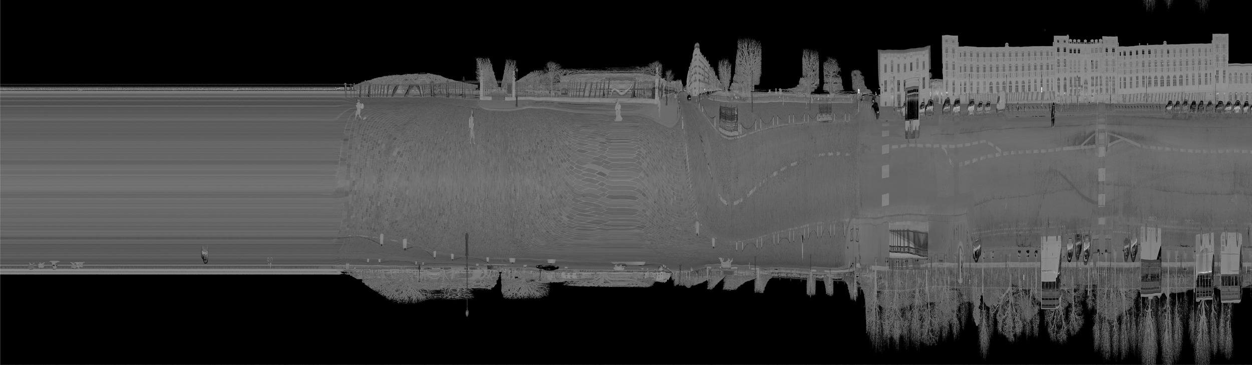
Figure 1: Echo intensity of a MLS displayed in sensor topology: vertical axis is the angle $\theta$, horizontal axis is the line number, equivalent to time as the scanner acquires a constant number of lines per second. Horizontal resolution depends on vehicle speed (the left part is constant because the vehicle is stopped).

In practice, existing surface reconstruction algorithms often consider that their input is a set of $(x,y,z)$ coordinates, possibly with normals. However, most LiDAR scanning technologies provide more than that: the sensors have a logic of acquisition that provides a sensor topology (Xiao et al.,, 2013; Vallet et al.,, 2015). For instance, planar scanners acquire points along a line that advances with the platform (plane, car, …) it is mounted on. Thus each point can be naturally connected to the one before and after him along the line, and to its equivalent in the previous and next lines (see Figure 1). Fixed LiDARs scan in spherical $(\theta,\phi)$ coordinates which also imply a natural connection of each point to the previous and next along these two angles. Some scanner manufacturers exploit this topology by proposing visualization and processing tools in 2.5D (depth images in $(\theta,\phi)$) rather than 3D. Moreover, LiDAR scanning can provide a meaningful information that is the position of the LiDAR sensor for each points, resulting in a ray along which we are sure that space is empty. This information can also disambiguate surface reconstruction as illustrated in Figure 3. This is why we decided to investigate the use of the sensor topology inherent to a MLS, to perform a 3D reconstruction of a point cloud.

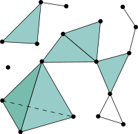
Figure 2: A simplicial complex consists of simplices of dimension 0 (points), 1 (edges) and 2 (triangles) (source Wikipedia)

Secondly, the geometry processing community has mainly focused on reconstruction of rather smooth objects, possibly with sharp edges, but with a sampling density sufficient to consider that the object is a 2-manifold, which means that it is locally 2-dimensional. Thus these methods do not extend well to real scenes where such a guarantee is hardly possible. In particular, scans including poles, power lines, wires, … almost never allow to create triangles on these structures because their widths (a few mm to a few cm) is much smaller than the scanning resolution. Scans of highly detailed structures (such as tree foliage for instance) even have a 0-dimensional nature: individual points should not even be connected to any of their neighbors. Applying the Nyquist-Shannon theorem to the the range in sensor space tells us that if the geometric frequency (frequency of the range signal in sensor space) is higher than half the sampling frequency (frequency of the samples in sensor space), then some (geometric) signal will be lost, which happens in the cases stated above for instance. Because of this, we should aim at reconstructing triangles only when the Shannon condition is met in the two dimensions, but only edges when the geometric frequency is too high in 1 dimension and points when the geometric frequency is too high in the 2 dimensions. Triangles, edges and points are called simplices, which are characterized by their dimension $d$ ($0=$ vertices, $1=$ edges, $2=$ triangles). If we add the constraint that edges can only meet at a vertex and triangles can only meet at an edge or vertex, the resulting mathematical object is called a simplicial complex as illustrated in Figure 2. The aim of this paper is to propose a method to reconstruct such simplicial complexes from a LiDAR scan.

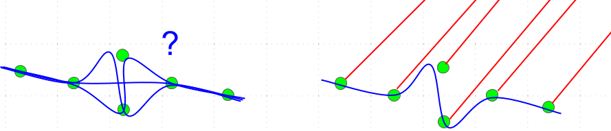
Figure 3: Left: a 2D point cloud (green) and possible reconstructions (blue). Right: knowing the LiDAR rays allows to solve the ambiguity

2 State of the art

3D surface mesh reconstruction from point clouds has been a major issue in geometry processing for the last decades. 3D reconstruction can be performed from oriented (Kazhdan and Hoppe,, 2013) or unoriented point sets (Alliez et al.,, 2007). Data itself can come from various sources: Terrestrial Laser Scanning (Pu and Vosselman,, 2009), Aerial Laser Scanning (Dorninger and Pfeifer,, 2008) or Mobile Laser Scanning. We refer the reader to Berger et al., (2014) for a general review of surface reconstruction methodologies and focus our state of the art on surface reconstruction from Mobile Laser Scanning (MLS) and on simplicial complexes reconstruction, which are the two specificities of our approach.

MLS have been used for the past years mostly for the modeling of outdoors environments, usually in urban scenes. Becker and Haala, (2009) propose an automatically-generated grammar for the reconstruction buildings, whereas Rutzinger et al., (2010) focus more specifically on tree shapes reconstruction. MLS has also been useful for specific indoor environments: Zlot and Bosse, (2014) used a MLS in an underground mine to obtain a 3D model of the tunnels.

The utility of simplicial complexes for the reconstruction of 3D point clouds has been expressed by Popović and Hoppe, (1997) as a generalization manner to simplify 3D meshes. Simplicial complexes are also used to simplify defect-laden point sets as a way to be robust to noise and outliers using optimal transport (De Goes et al.,, 2011; Digne et al.,, 2014) or alpha-shapes (Bernardini and Bajaj,, 1997).

As explained in introduction, the aim of this paper is to propose a reconstruction method that combines two advantages:

1. Reconstruction of a simplicial complexe instead of a surface mesh, adapting the local dimension to that of the local structure.

2. Exploiting the sensor topology both to solve ambiguities and to speed up computations.

The two objectives are tackled at once by proposing a new criteria to define which simplices from the sensor topology should belong to the reconstructed simplicial complex.

3 Methodology

As explained above, sensor topology yields in general a regular mesh structure with a 6-neighborhood that can be used to perform a surface mesh reconstruction. This reconstruction is however very poor as all depth discontinuities will be meshed, so very elongated triangles will be constructed between objects and their background. This section investigates criteria to remove these triangles, while possibly keeping some of their edges. As all input points will be kept, the resulting reconstruction combines points and edges and triangles based on these points, which is called a simplicial complex in mathematics.

3.1 Objectives

Our main objective is to determine which adjacent points (in sensor topology) should be connected to form edges and triangles. We consider that we may be facing a discontinuity when the depth difference between two neighboring echoes is high. This depth difference is computed from a sensor viewpoint, which implies that a large depth difference may correspond to two cases: either the echoes fell on two different objects with a notable depth difference, or they fell on a grazing surface (nearly parallel to the laser beams direction) as shown in figure 4. When two neighboring echoes have a large depth difference, there is no way we can guess whether they are located on two separate objects (4(a)) or a grazing surface (4(b)). The core idea of our filtering is that the only hint we can rely on to distinguish between these two cases is that if at least three echoes with a large depth differences are aligned (4(c)), we probably are in the grazing surface case rather than on separate objects.

To perform our reconstruction, we consider each echo as an independent point. First, we define a neighborhood relationship between echoes in the sensor topology. Then, we create edges, based on the echoes and add triangles based on the edges. Last, we regularize the computed simplicial complex according to the local geometric consistency of the retrieved simplexes.

(a) Separation case

(b) Ambiguous case

(c) Non-separation case

Figure 4: Illustration of the two cases of important depth difference. The arrows represent the laser beams. Figures 4(a) and 4(b) show the cases where two neighboring echoes have a huge depth difference. They can either fall on two different objects or on a same object and we have no hint to distinguish these two cases. Figure 4(c) shows the case where three or more echoes are approximately aligned, with a huge depth difference. In this case we want to reconstruct edges between these echoes because it may correspond to a grazing surface.

3.2 Neighborhood in sensor topology

The sensors used to capture point clouds often have an inherent topology. Mobile Laser Scanners sample a regular grid in ($\theta,t$) where $\theta$ is the rotation angle of the laser beam and $t$ the instant of acquisition. Because the vehicle moves at a varying speed (to adapt to the traffic and respect the circulation rules) and may rotate, the sampling is however not uniform in space. In general, the number $N_{p}$ of pulses for a 2$\pi$ rotation in $\theta$ is not an integer so a pulse $P_{i}$ has six neighbors $P_{i-1}$, $P_{i+1}$, $P_{i-n}$, $P_{i-n-1}$, $P_{i+n}$, $P_{i+n+1}$ where $n=\lfloor N_{p}\rfloor$ is the integer part of the number of pulses per line as illustrated on figure 5(a).

However, this topology concerns emitted pulses, not recorded echoes. One pulse might have 0 echo (no target hit) or up to 8 as most modern scanners can record multiple echoes for one pulse if the laser beam intersected several targets, which is very frequent in the vegetation or transparent objects for instance. We chose to tackle this issue by connecting an echo to each echoes of its pulses’ neighbors as illustrated in Figure 5(b) because we should keep all possible edge hypotheses before filtering them.

(a) The pulse sensor topology forms a 6-neighborhood

(b) Echo sensor topology: each echo is connected to all echoes of all neighboring pulses

Figure 5: Definition of neighborhood in sensor space. For each figure, the points considered is colored in red, and connection is denoted by a red arrow.

3.3 Edge filtering

For each pair of connected echoes in sensor topology (as defined above), we need a criteria to decide whether we should keep it in the reconstructed simplicial complex. We propose the following:

• $C_{0}$ regularity: we want to prevent forming edges between echoes when their euclidean distance is too high.

• $C_{1}$ regularity: we want to favor edges when two collinear edges share an echo.

In order to be independent from the sampling density, we propose to express the regularities in an angular manner. Moreover, the sensor topology has an hexagonal structure, and we propose to treat each line in the 3 directions of the structure independently. For the reminder of this article, and because a single pulse can have multiple echoes, we will express, for a pulse ${p}$, its echoes as $E_{p}^{e}$ where ${e}\in 1\ldots N_{p}$, with ${N_{p}}$ the number of echoes of ${p}$. We then express the regularities as:

• $C_{0}$ regularity, for an edge $(E_{p}^{e_{1}},E_{p+1}^{e_{2}})$ between two echoes of two neighboring pulses:

  $$C_{0}(\mathit{p},e_{1},e_{2})=1-\vec{e_{p}}(e_{1},e_{2})\cdot\vec{l_{p}}\quad,$$

  where $\vec{e_{p}}(e_{1},e_{2})=\frac{\overrightarrow{E_{p}^{e_{1}}E_{p+1}^{e_{2}}}}{||\overrightarrow{E_{p}^{e_{1}}E_{p+1}^{e_{2}}}||}$ and $\vec{l_{p}}$ is the direction of the laser beam of pulse $p$ (cf Figure 6). $C_{0}$ is close to 0 for surfaces orthogonal to the LiDAR ray and close to 1 for grazing surfaces, almost parallel to the ray.

• $C_{1}$ regularity, for an edge $(E_{p}^{e_{1}},E_{p+1}^{e_{2}})$ between two echoes of two neighboring pulses:

  $$\begin{split}C_{1}(p,e_{1},e_{2})\!=\,&min_{e=1}^{N_{p-1}}|1-\vec{e}_{p-1}(e,e_{1})\cdot\vec{e}_{p}(e_{1},e_{2})|\cdot\\ &min_{e=1}^{N_{p+2}}|1-\vec{e}_{p}(e_{1},e_{2})\cdot\vec{e}_{p+1}(e_{2},e)|.\end{split}$$

  where the minima are given a value of 1 if the pulse is empty. $C_{1}$ is close to 0 is the edge is aligned with at least one of its neighboring edges, and close to 1 if it is orthogonal to all neighboring edges.

Figure 6: Illustration of the computed regularities $C_{0}$ and $C_{1}$. The black dots represent the echoes associated to the considered pulses. The blue and red ones correspond respectively to the precedent and following adjacent echoes. The solid arrows show the adjacent echoes used for the $C_{0}$ and $C_{1}$ computation. The black one correspond to the most orthogonal liaison to the sensor beams. The blue and red ones are selected because the angle between these vectors and the black one are the closest possible to $\pi$. The black dashed lines represent the laser beams.

From these regularities, we propose a simple filtering based on the computed angles. Figure 6 illustrates the computation of the $C_{0}$ and $C_{1}$ regularities. Considering two adjacent echoes $E^{e_{1}}_{p}$ and $E^{e_{2}}_{p+1}$, the $C_{0}$ regularity can be interpreted as the cosine of the angle between the laser beam direction in $p$ and $\vec{e_{p}}(e_{1},e_{2})$. We want to favor low values of the $C_{0}$ as it corresponds to echoes with a low depth difference. On the other side, to compute the $C_{1}$ regularity, we have to browse the echoes of the preceding and following pulses along the 3 directions of our structure. For the preceding and following pulses, we select the echo which minimizes $\mid 1-\vec{e_{p-1}}(e,e_{1})\cdot\vec{e_{p}}(e_{1},e_{2})\mid$ (respectively $\mid 1-\vec{e_{p+1}}(e_{2},e)\cdot\vec{e_{p}}(e_{1},e_{2})\mid$). This gives us an information about the tendency of the considered edge to be collinear with at least one of its adjacent edges. We will favor the most collinear cases.

Given two adjacent echoes, we consider that if the $C_{0}$ regularity is high enough, we can ensure the real existence of the edge, and don’t have to compute the $C_{1}$ regularity. We denote this threshold $\alpha_{m}$. For all the other cases, we compute the $C_{1}$ regularity and filter the edges according to the $C_{0}$ and $\alpha_{m}$:

$$C_{1}<\frac{\lambda\cdot\alpha_{m}\cdot C_{0}}{\alpha_{m}-C_{0}}\quad,$$

where $\lambda$ sets how much $C_{1}$ regularity can compensate for $C_{0}$ discontinuity. A high value of $\lambda$ allows more edges to be kept. This criteria is illustrated on figure 7. The red line represent the $\alpha_{m}$ threshold and the blue line corresponds to the limit cases between removing and keeping the edges depending on $C_{0}$ and $C_{1}$.

Figure 7: Filtering of edges knowing $C_{0}$ and $C_{1}$. The red line corresponds to the $\alpha_{m}$ threshold on $C_{0}$. The hatched area corresponds to the edges that we keep.

We also want to filter edges that would remain single in the cloud, or just connected to one other edge but with different directions. Actually this often occurs on noisy areas where an edge can pass the regularity criteria "by chance", but it is very unprobable that this happens for two neighboring edges. That’s why we propose an additional criterion to favor a reconstruction that leaves points instead of isolated or unaligned edges.

Let $e$ be an edge and $\left\{e_{1},\ldots,e_{n}\right\}$ its adjacent edges. We consider that if we find an edge $e_{i}\in\left\{e_{1},\ldots,e_{n}\right\}$ so that:

$$1-\vec{e}\cdot\vec{e_{i}}<\epsilon\quad,$$

where $\epsilon$ is the tolerance on edge reconstruction, $e$ is not alone or unaligned and we keep it in the simplicial complex.

3.4 Triangle filtering

Once we obtained a set of edges in our point cloud, a simple approach to filter triangles is to keep only the triangles (from sensor topology) which three edges have survived the edge filtering described above. Even if this method is an easy way to retrieve most triangles of the scene, it prevents recovering triangles in areas where edges are close to the threshold, in which case triangles will often have some edges just below and some just above the threshold so most triangles will be filtered out.

In order to regularize the triangulation computed, we want to favor triangles that are coplanar to some of their adjacent triangles, in the same way we favored edges aligned with at least one neighboring edge. This is motivated by the fact that we want to ensure spatial regularity in our scene. Moreover, we found very unlikely the cases where a triangle is left alone. Also we want to remove all the triangles that may be formed by edges in noisy parts of the cloud as we cannot ensure their existence in the real scene.

As triangles are 2D objects, we want to define a 2D $C_{1}$ regularity by separating between $C_{1}$ regularity along two directions. Unfortunately, a triangle has 3 neighbors. We solve the problem by filtering pairs of adjacent triangles (that we will call wedges) which have four adjacent wedges in 2 separate directions as illustrated on figure 8.

Figure 8: Representation of a wedge (red) and its adjacent wedges. The limit between the triangles of each wedge is represented with a dotted line. The dashed lines stand for the directions of our structure. Wedges adjacent to the red one are numbered from 1 to 4.

The filtering we propose to keep the wedges that are $C_{1}$ regular with neighboring wedges in the two directions, where $C_{1}$ regularity is defined as the criterion:

$$1-|W^{N}\cdot W_{i}^{N}|<\omega\quad,$$

where $W$ is a wedge whose normal is $W^{N}$ and $\left\{W_{1},\ldots,W_{n}\right\}$ are its adjacent wedges whose normals are $\left\{W_{1}^{N},\ldots,W_{n}^{N}\right\}$ respectively. This means, on figure 8, that if the red wedge is only $C_{1}$ regular with the wedges 1 and 3, it will be discarded, while it will be kept if it is regular with only 1 and 2. $\omega$ is the tolerance on the co-planarity of the two wedges to define regularity. The rationale behind this choice is the same as for the edges: being irregular with both neighbors in one direction means that we are on a depth discontinuity in that direction that cannot be distinguished from a grazing surface, while regularity with at least one neighbor in both directions means that the wedge is part of a (potentially grazing) planar surface.

4 Results

We implemented the pipeline presented before, first with only the edge filtering and the simple triangle reconstruction from edge effectively forming a triangle. Then we added the triangle filtering part. We compared our results with a naive filtering on edge length where triangles in the simplicial complex correspond to all triplets of edges forming a triangle.

For all the following tests, we used data from the Stereopolis vehicle (Paparoditis et al.,, 2012). The scenes have been acquired in an urban environment (Paris) and are mostly composed of roads, facades, trees and urban planning. All the simplicial complexes presented in this part will be represented as follow:

• triangles in red,

• edges that are not part of any triangle in green,

• points that don’t belong to any triangle or edge in black.

Note that following its mathematical definition, the endpoints of an edge of a simplicial complex also belong to the complex, and similarly for the edges of a triangle, but we do not display them for clarity.

The parameter search phase was conducted in two experiments. In the first set of experiments, the impact of parameters $\alpha_{m}$ and $\lambda$ were studied. For the remaining parameters $\omega$ and $\epsilon$, their influence was tested in a second batch of experiments. Because all our criteria depend on trigonometric functions (the dot products of normalized vectors is the cosine of their angle), all these parameters are to choose in $[0,1]$. Last, we compare both methods with the naive filtering on edge length.

4.1 Parametrization of $\alpha_{m}$ and $\lambda$

We first studied the influence of $\alpha_{m}$. A high value will discard a lot of edges and prevent the formation of triangles, whereas a low value will preserve too many edges on real discontinuities. The results are presented in figure 9. We see on the left example that on the one hand, low values of $\alpha_{m}$ allow the formation of edges between the bottom of the traffic sign and the road. On the other hand, high values of $\alpha_{m}$ show that the reconstruction of triangles is harder, even on the road.

The second parameter of this method, $\lambda$ corresponds to the fact that we want to preserve grazing surfaces where edges are long (important depth discontinuity) but collinear. Figure 10 illustrates the tuning of this $\lambda$ parameter. On the one hand, for high values of $\lambda$ (right), edges between window bars and walls or insides of buildings are created. On the other hand, when $\lambda$ is too low (left), only the best edges are retrieved. For these cases, the number of remaining edges is low (hundreds of edges for millions of points), and lowering $\lambda$ removes edges that may be useful for human interpretation of the reconstruction.

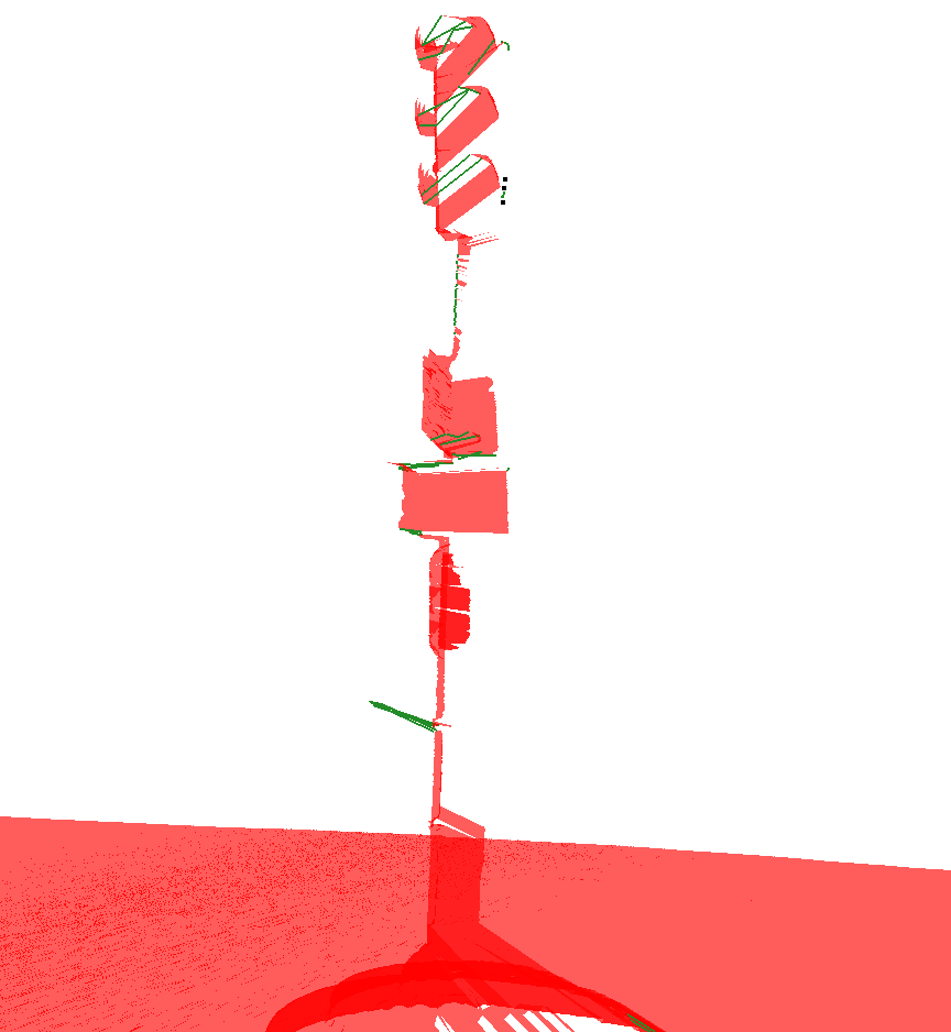
(a) $\alpha_{m}$= 0.01

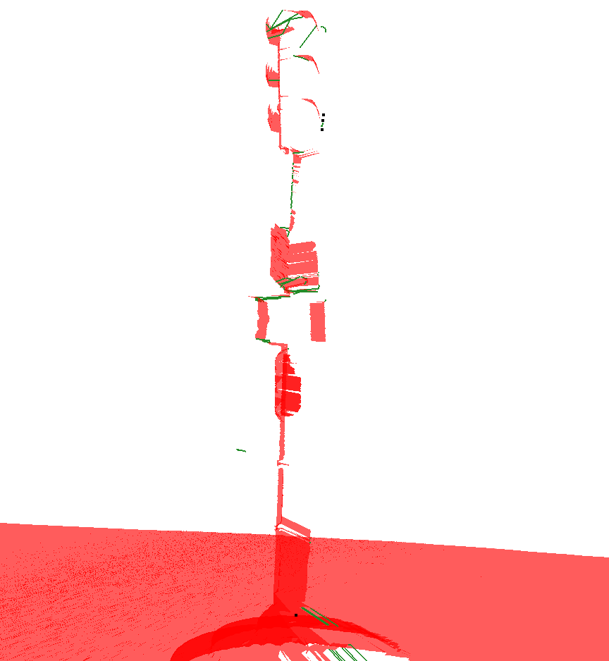
(b) $\alpha_{m}$= 0.05

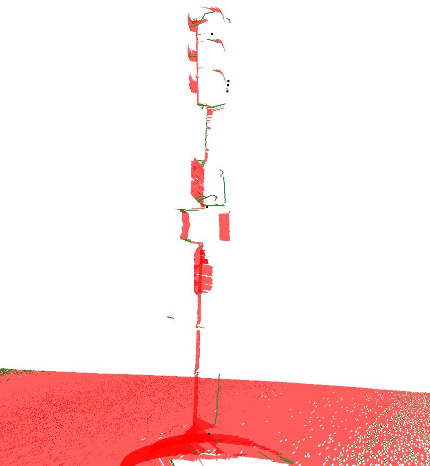
(c) $\alpha_{m}$= 0.1

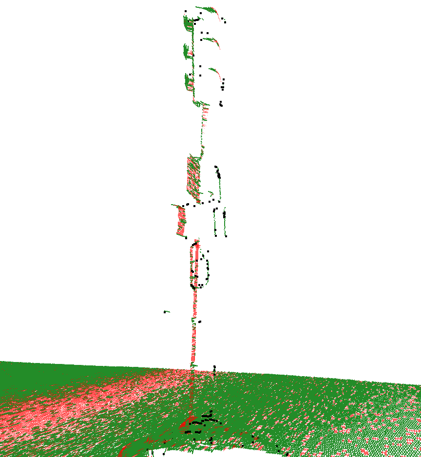
(d) $\alpha_{m}$= 0.5

Figure 9: Influence of $\alpha_{m}$. $\lambda$ is fixed to $10^{-4}$.

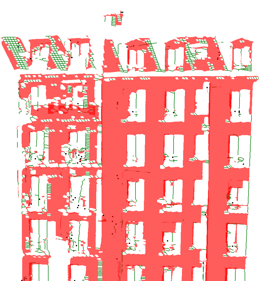
(a) $\lambda=10^{-6}$

(b) $\lambda=10^{-4}$

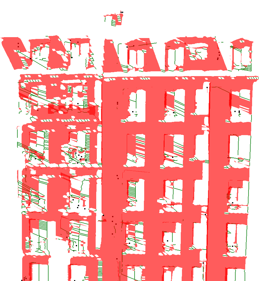
(c) $\lambda=10^{-2}$

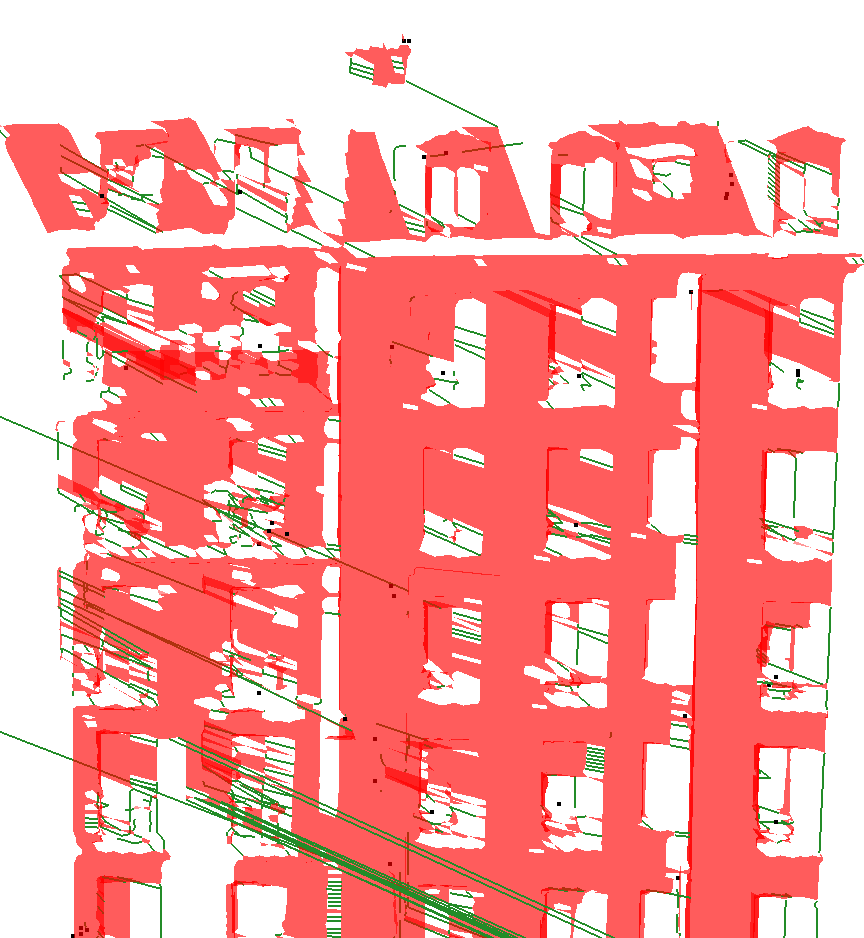
(d) $\lambda=0.1$

Figure 10: Influence of $\lambda$. $\alpha_{m}$ is fixed to 0,05. The scene represents a facade in the grazing surface case.

4.2 Parametrization of $\omega$ and $\epsilon$

For this set of experiments, $\alpha_{m}$ and $\lambda$ were fixed respectively to $0.05$ and $10^{-4}$. The influence of the last two parameters is especially visible on noisy areas and grazing surfaces, where the level of detail of the scene is close to the acquisition density. We first studied the effect of parameter $\omega$ on triangles. For high values of $\omega$, we expect that a lot of triangles will be retrieved, especially in the grazing surface case, where sometimes our algorithm struggles to retrieve edges in the 3 directions (but performs well on two directions). The results are shown on figure 11 and illustrate our problem in the grazing surface case. The figure on the left is the baseline computed previously. As expected, the number of triangles increase for high values of $\omega$ and the road is cleaner than without the triangle filtering part. Its main drawback is its propensity to let a few triangles in noisy areas like tree’s foliage.

The second parameter $\epsilon$ is a regularization term on the edges. Low values of $\epsilon$ will decrease the number of edges, thus leaving many points not linked to others. Results are presented in figure 12. As previously, the figure on the left shows the output of the first filtering step. Figures corresponding to lowest values of $\epsilon$ respect our previsions: the number of edges keeps decreasing whereas the number of points increase. A side effect of this method can be seen on figure 12(b), as there is nearly no edge in the tree’s foliage.

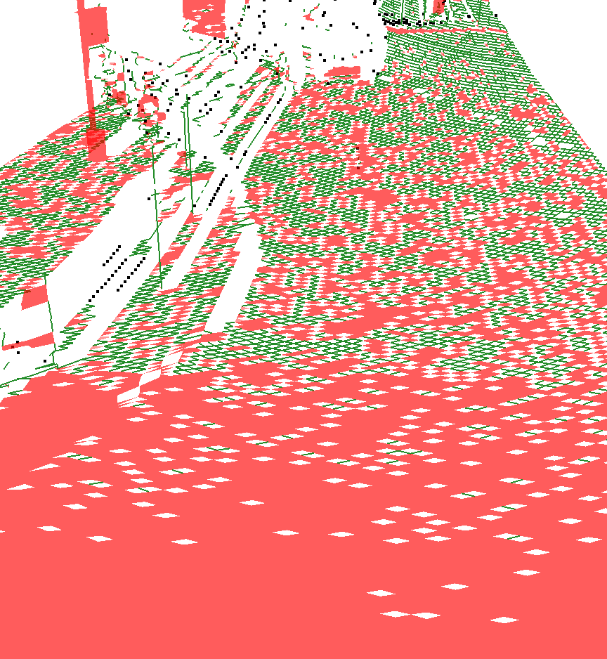
(a) No triangle filtering

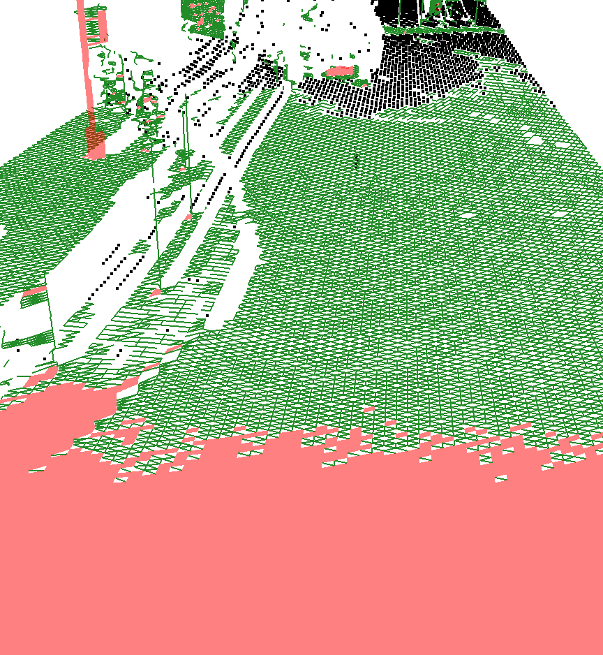
(b) $\omega=10^{-5}$

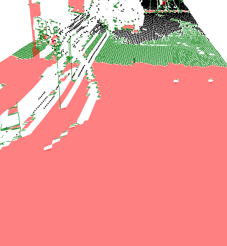
(c) $\omega=10^{-4}$

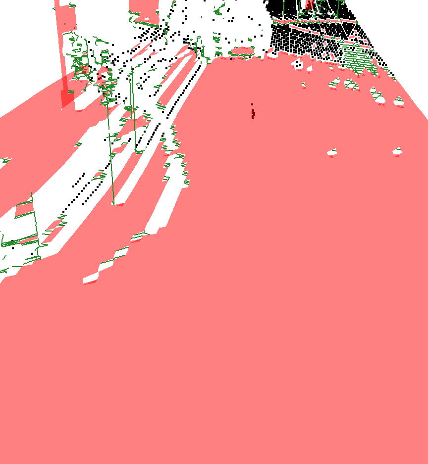
(d) $\omega=10^{-3}$

Figure 11: Parametrization of $\omega$. $\epsilon$ is fixed to $5\cdot 10^{-3}$. The scene represents a road in the grazing surface case.

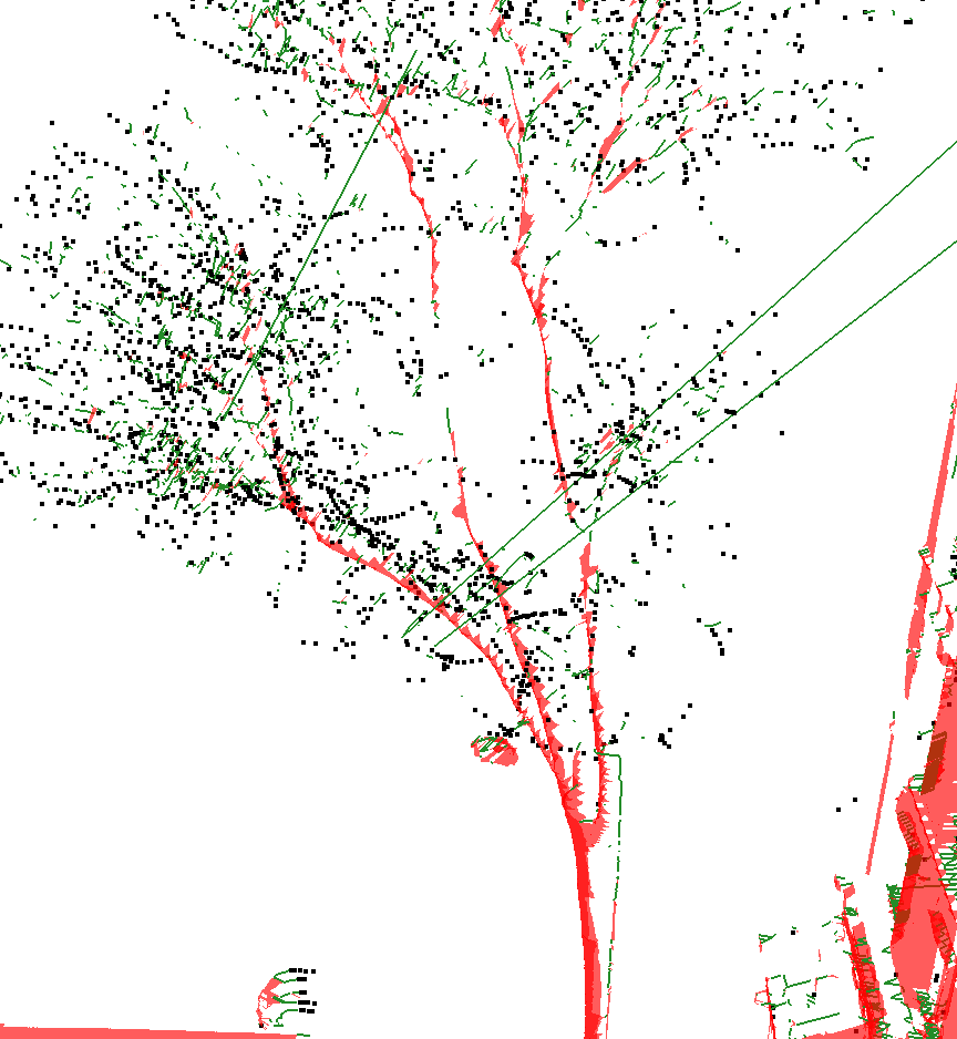
(a) No triangle filtering

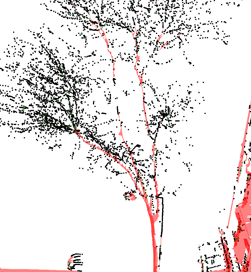
(b) $\epsilon=10^{-5}$

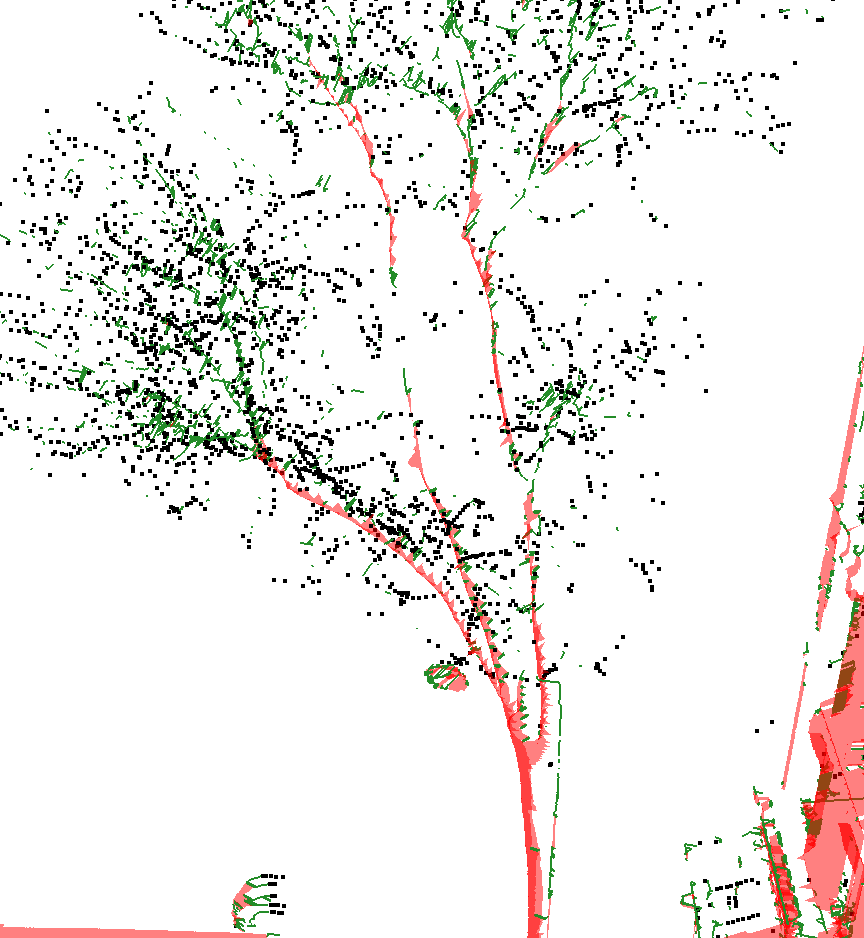
(c) $\epsilon\!\!=\!\!5\cdot 10^{-3}$

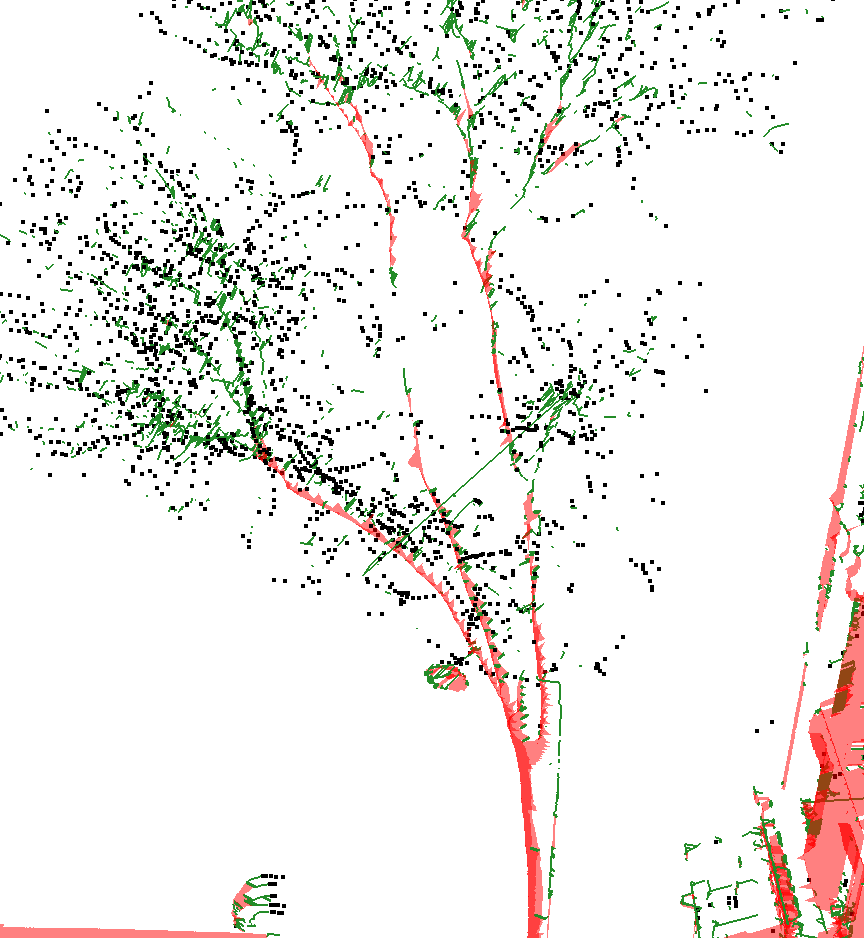
(d) $\epsilon=10^{-2}$

Figure 12: Parametrization of $\epsilon$. $\omega$ is fixed to $10^{-3}$. The scene represents a tree with its foliage.

4.3 Comparison of the three methods

In this part, we compare our two methods to a naive filtering based on edge lengths alone. The naive filtering is based on a $0.5$ meters threshold. For both methods, $\alpha_{m}$ and $\lambda$ are respectively fixed to $0.05$ and $10^{-4}$. Furthermore, for the last method, $\omega$ and $\epsilon$ are fixed to $10^{-3}$ and $5\cdot 10^{-3}$ respectively. A video of the results is available at (Guinard, n.d., ).

Figure 13 presents a reconstruction in a complex urban scene. Unlike the naive filtering, our methods are able to retrieve thin objects such as poles or windows bars without merging them to the closest objects. This is illustrated on figure 13. The top right image of this figure is an extract from Google Streetview to help the interpretation.

Figure 14 focus more on specific areas of the scan. The first row shows the naive filtering method, whereas the second and third rows present respectively the edge filtering method and its extension with the triangle filtering. We remark that the naive filtering method struggles to retrieve limits between objects (like between poles and road, or people and buildings). The main advantage of the triangle filtering over the edge filtering that can be seen here, is that it helps to reduce the noise that occurs in complex areas such as tree foliage or grazing surfaces. We assume that in complex areas we cannot ensure the existence of connections between some points and will favor a reconstruction that remains careful on such areas. This is why the last method, which is less noisy than the edge filtering, is considered a more appropriate baseline for further developments, even if it discards some edges or triangles that had been well retrieved by the edge filtering method on grazing surfaces.

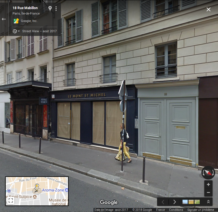
(a) Image of the scene from Google, n.d.

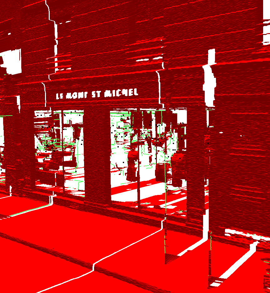
(b) Naive method

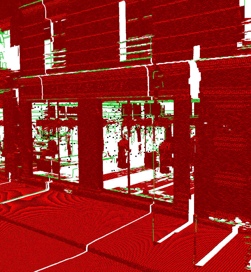
(c) Edge filtering

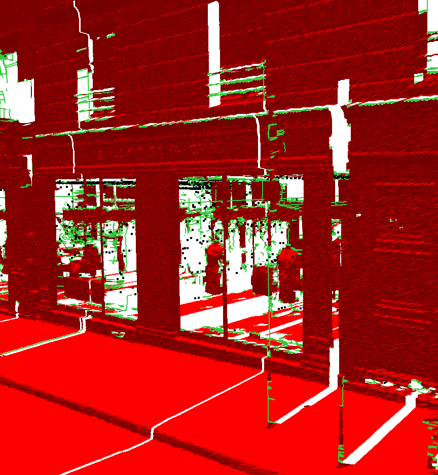
(d) Triangle filtering

Figure 13: Results on a complete urban scene, with road, facades, poles and pedestrians.

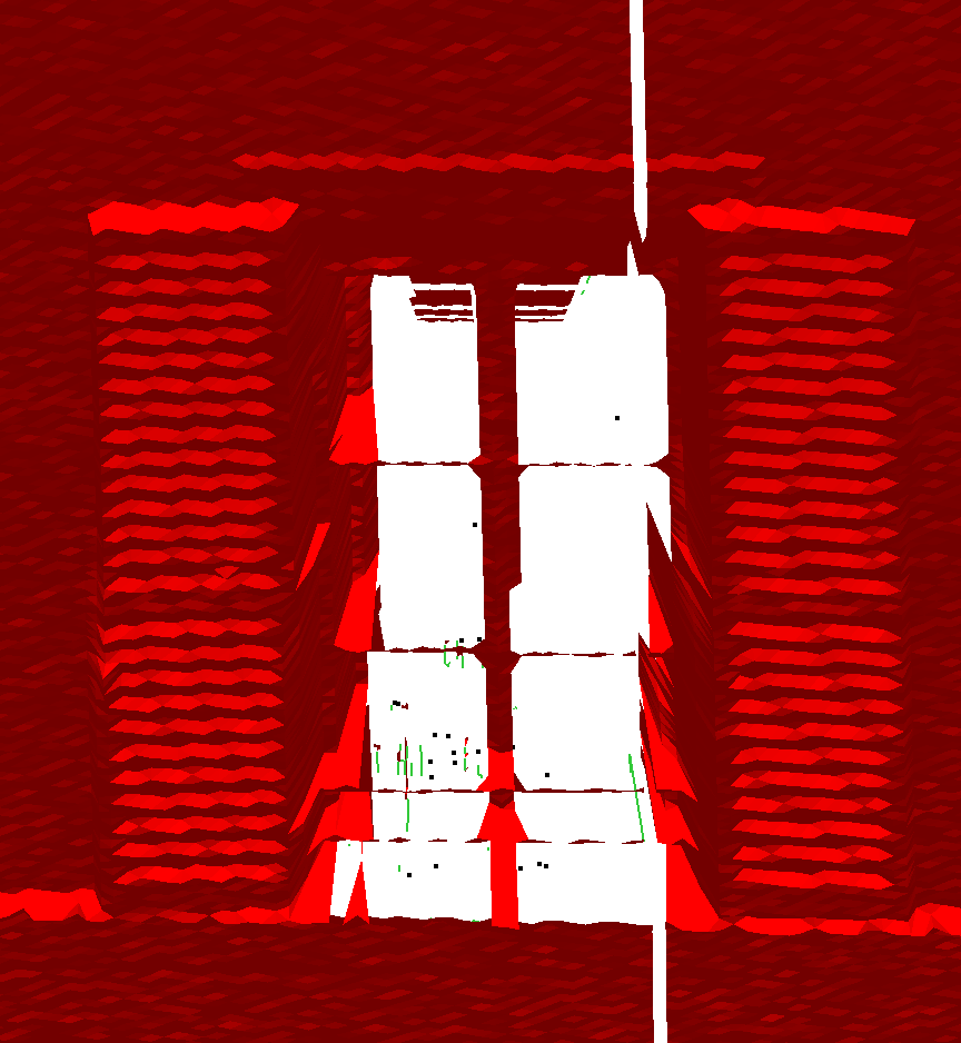
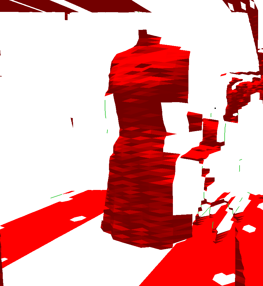
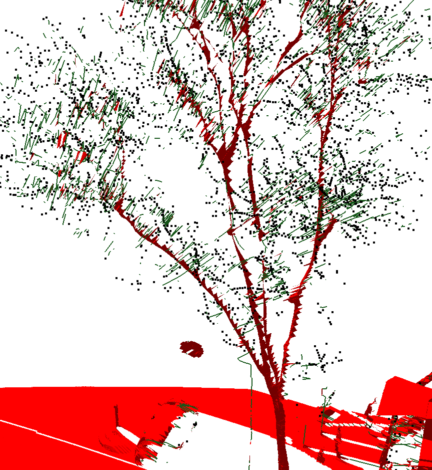
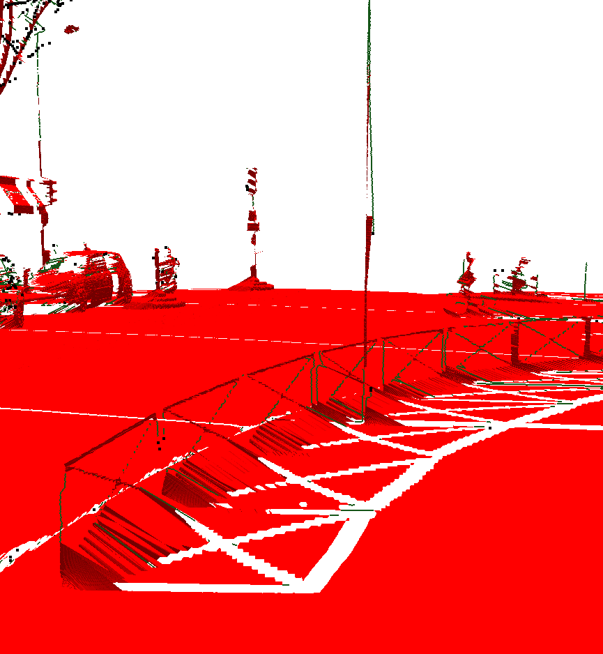
(a) Naive filtering

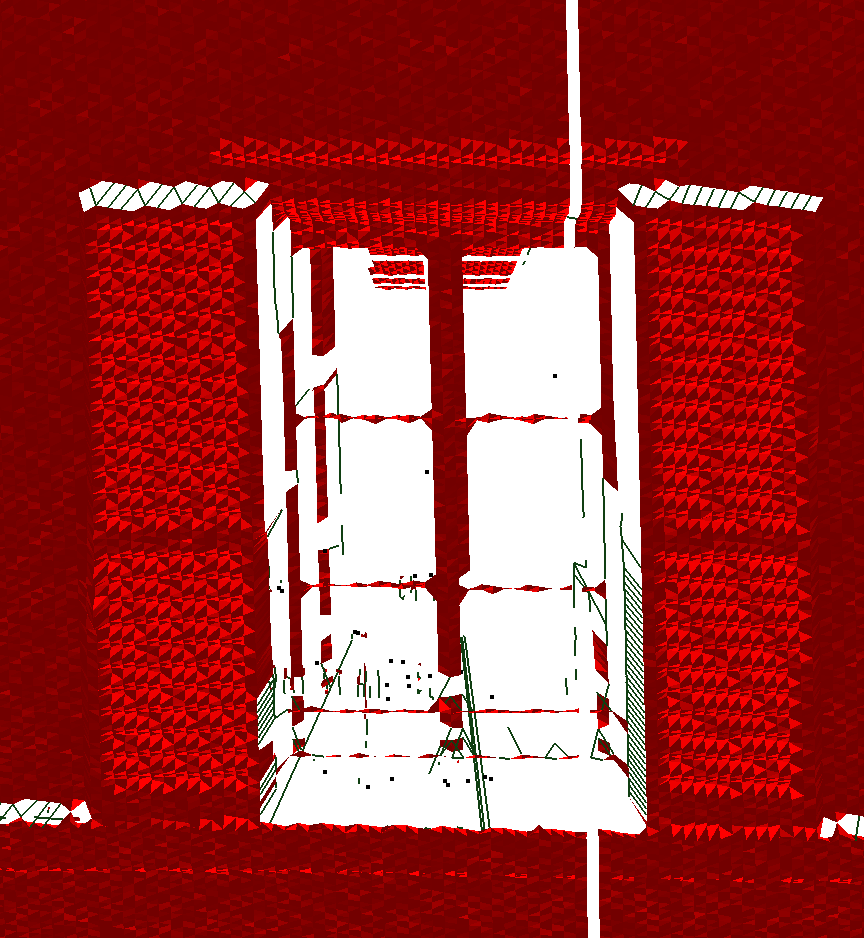
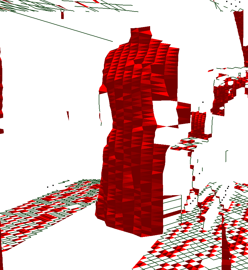
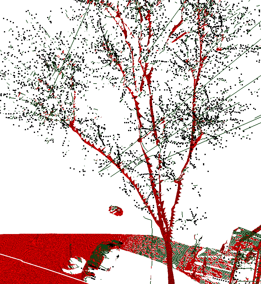
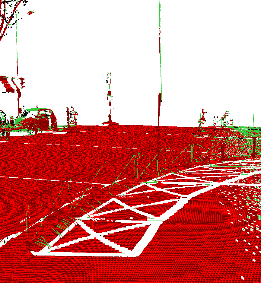
(b) Edge filtering

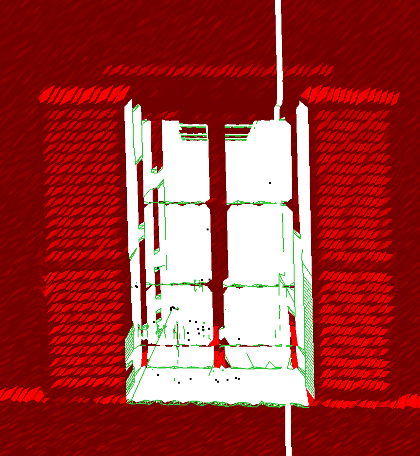
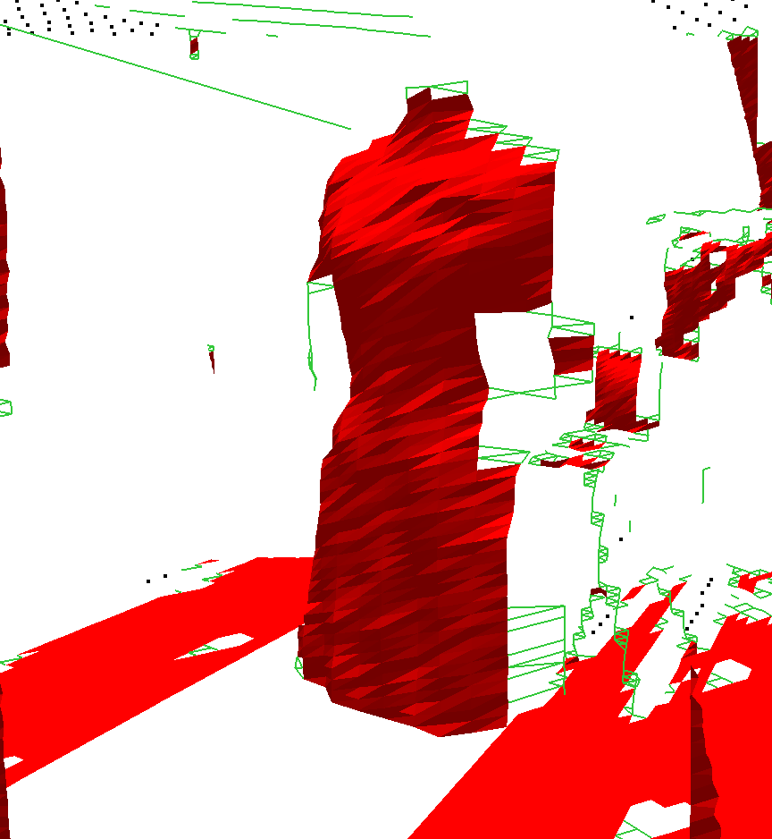
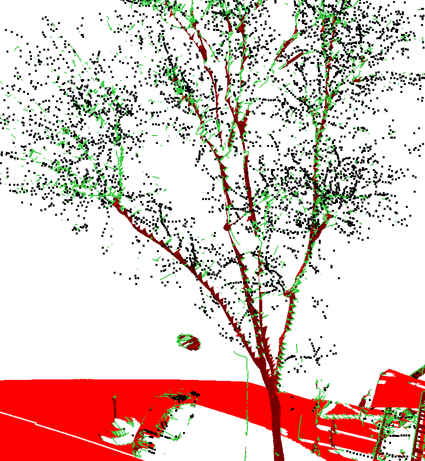
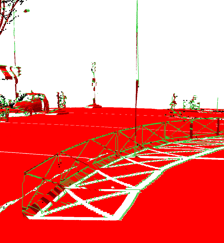
(c) Triangle Filtering

Figure 14: Comparison of the three methods: the naive filtering, the edge filtering and its extension with the triangle filtering. From left to right, the scenes represent: a window, a model in a showcase, a tree and barriers on a pavement.

5 Conclusions and perspectives

This article presented a method for the simplicial complexes reconstruction of point clouds from MLS, based on the inherent structure of the MLS. We propose a filtering of edges possibly linking adjacent echoes by searching for collinear edges in the cloud, or edges perpendicular to the laser beams. We also presented an improvement of this method as a second filtering step, this time by looking for coplanar triangles. This last method produced simplicial complexes less holed than our first approach, and respects the noisy areas of the cloud (such as tree foliage) by discarding simplexes which existence cannot be ensured.

The main drawback of our methods is its high locality: we work only by considering point’s neighbors and simplexes’ adjacent simplexes. Using knowledge of the neighbors at different scales, or even on the whole cloud could help us to regularize the reconstruction according to more global structures of the cloud. Further developments may also consider a hole filling process, to get rid of the absence of a few missing simplexes in a large structure (road, building). Last, setting up a generalization method, as in Popović and Hoppe, (1997), would be interesting to simplify the resulting simplicial complexes on large and regular structures in order to reduce the memory weight of the simplicial complexes while maintaining a high accuracy.

References

References

- Alliez et al., (2007) Alliez, P., Cohen-Steiner, D., Tong, Y. and Desbrun, M., 2007. Voronoi-based variational reconstruction of unoriented point sets. In: Symposium on Geometry processing, Vol. 7, pp. 39–48.
- Becker and Haala, (2009) Becker, S. and Haala, N., 2009. Grammar supported facade reconstruction from mobile lidar mapping. In: ISPRS Workshop, CMRT09-City Models, Roads and Traffic, Vol. 38, p. 13.
- Berger et al., (2014) Berger, M., Tagliasacchi, A., Seversky, L., Alliez, P., Levine, J., Sharf, A. and Silva, C., 2014. State of the art in surface reconstruction from point clouds. In: EUROGRAPHICS star reports, Vol. 1number 1, pp. 161–185.
- Bernardini and Bajaj, (1997) Bernardini, F. and Bajaj, C. L., 1997. Sampling and reconstructing manifolds using alpha-shapes. In: In Proc. 9th Canad. Conf. Comput. Geom, Citeseer.
- De Goes et al., (2011) De Goes, F., Cohen-Steiner, D., Alliez, P. and Desbrun, M., 2011. An optimal transport approach to robust reconstruction and simplification of 2D shapes. In: Computer Graphics Forum, Vol. 30number 5, Wiley Online Library, pp. 1593–1602.
- Digne et al., (2014) Digne, J., Cohen-Steiner, D., Alliez, P., De Goes, F. and Desbrun, M., 2014. Feature-preserving surface reconstruction and simplification from defect-laden point sets. Journal of mathematical imaging and vision 48(2), pp. 369–382.
- Dorninger and Pfeifer, (2008) Dorninger, P. and Pfeifer, N., 2008. A comprehensive automated 3D approach for building extraction, reconstruction, and regularization from airborne laser scanning point clouds. Sensors 8(11), pp. 7323–7343.
- (8) Google, n.d. View of the Mabillon street next to the corner of Lobineau street (Paris). https://goo.gl/maps/FQTvA7oaiNm [Accessed: 2018-01-09].
- (9) Guinard, S., n.d. Sensor-topology based simplicial complex reconstruction from mobile laser scanning. https://youtu.be/zJn3YF8eer4 [Accessed: 2018-04-06].
- Kazhdan and Hoppe, (2013) Kazhdan, M. and Hoppe, H., 2013. Screened poisson surface reconstruction. ACM Transactions on Graphics (TOG) 32(3), pp. 29.
- Paparoditis et al., (2012) Paparoditis, N., Papelard, J.-P., Cannelle, B., Devaux, A., Soheilian, B., David, N. and Houzay, E., 2012. Stereopolis II: A multi-purpose and multi-sensor 3d mobile mapping system for street visualisation and 3d metrology. Revue française de photogrammétrie et de télédétection 200(1), pp. 69–79.
- Popović and Hoppe, (1997) Popović, J. and Hoppe, H., 1997. Progressive simplicial complexes. In: Proceedings of the 24th annual conference on Computer graphics and interactive techniques, ACM Press/Addison-Wesley Publishing Co., pp. 217–224.
- Pu and Vosselman, (2009) Pu, S. and Vosselman, G., 2009. Knowledge based reconstruction of building models from terrestrial laser scanning data. ISPRS Journal of Photogrammetry and Remote Sensing 64(6), pp. 575–584.
- Rutzinger et al., (2010) Rutzinger, M., Pratihast, A., Oude Elberink, S. and Vosselman, G., 2010. Detection and modelling of 3D trees from mobile laser scanning data. Int. Arch. Photogramm. Remote Sens. Spat. Inf. Sci 38, pp. 520–525.
- Vallet et al., (2015) Vallet, B., Brédif, M., Serna, A., Marcotegui, B. and Paparoditis, N., 2015. TerraMobilita/iQmulus urban point cloud analysis benchmark. Computers & Graphics 49, pp. 126–133.
- Xiao et al., (2013) Xiao, W., Vallet, B. and Paparoditis, N., 2013. Change detection in 3D point clouds acquired by a mobile mapping system. ISPRS Annals of Photogrammetry, Remote Sensing and Spatial Information Sciences 1(2), pp. 331–336.
- Zlot and Bosse, (2014) Zlot, R. and Bosse, M., 2014. Efficient large-scale 3D mobile mapping and surface reconstruction of an underground mine. In: Field and service robotics, Springer, pp. 479–493.