Approximation Algorithms for Cascading Prediction Models

Abstract

We present an approximation algorithm that takes a pool of pre-trained models as input and produces from it a cascaded model with similar accuracy but lower average-case cost. Applied to state-of-the-art ImageNet classification models, this yields up to a 2x reduction in floating point multiplications, and up to a 6x reduction in average-case memory I/O. The auto-generated cascades exhibit intuitive properties, such as using lower-resolution input for easier images and requiring higher prediction confidence when using a computationally cheaper model.

1 Introduction

In any machine learning task, some examples are harder than others, and intuitively we should be able to get away with less computation on easier examples. Doing so has the potential to reduce serving costs in the cloud as well as energy usage on-device, which is important in a wide variety of applications (Guan et al., 2017).

Following the tremendous empirical success of deep learning, much recent work has focused on making deep neural networks adaptive, typically via an end-to-end training approach in which the network learns to make example-dependent decisions as to which computations are performed during inference. At the same time, recent work on neural architecture search has demonstrated that optimizing over thousands of candidate model architectures can yield results that improve upon state-of-the-art architectures designed by humans (Zoph et al., 2017). It is natural to think that combining these ideas should lead to even better results, but how best to do so remains an open problem.

One of the motivations for our work is that for many problems, there are order-of-magnitude differences between the cost of a reasonably accurate model and that of a model with state-of-the-art accuracy. For example, the most accurate NasNet model achieves 82.7% accuracy on ImageNet using 23 billion multiplies per example, while a MobileNet model achieves 70.6% accuracy with only 569 million multiplies per example (Howard et al., 2017; Zoph et al., 2017). If we could identify the images on which the smaller model’s prediction is (with high probability) no less accurate than the larger one’s, we could use fewer multiplications on those images without giving up much accuracy.

In this work, we present a family of algorithms that can be used to create a cascaded model with the same accuracy as a specified reference model, but potentially lower average-case cost, where cost is user-defined. This family is defined by a meta-algorithm with various pluggable components. In its most basic instantiation, the algorithm takes a pool of pre-trained models as input and produces a cascaded model in two steps:

1. It equips each model with a set of possible rules for returning “don’t know” (denoted $\bot$) on examples where it is not confident. Each (model, rule) combination is called an abstaining model.

2. It selects a sequence of abstaining models to try, in order, when making a prediction (stopping once we find a model that does not return $\bot$).

We also present instantiations of the meta-algorithm that generate new prediction models on-the-fly, either using lightweight training of ensemble models or a full architecture search. We also discuss a variant that produces an adaptive policy tree rather than a fixed sequence of models.

An important feature of our algorithms is that they scale efficiently to a large number of models and (model, rule) combinations. They also allow for computations performed by one stage of the cascade to be re-used in later stages when possible (e.g., if two successive stages of the cascade are neural networks that share the same first $k$ layers).

2 Abstaining models

Our cascade-generation algorithm requires as input a set of abstaining models, which are prediction models that return “don’t know” (denoted $\bot$) on certain examples. For classification problems, such models are known as classifiers with a reject option, and methods for training them have been widely studied (Yuan & Wegkamp, 2010). In this section we present a simple post-processing approach that can be used to convert a pre-trained model from any domain into an abstaining model.

We assume our prediction model is a function $p:\mathcal{X}\rightarrow\mathcal{Y}$, and that its performance is judged by taking the expected value of an accuracy metric $q:\mathcal{Y}\times\mathcal{Y}\rightarrow\mathbb{R}$, where $q(\hat{y},y)$ is the accuracy of prediction $\hat{y}$ when the true label is $y$. Our goal is to create an abstaining model $m:\mathcal{X}\rightarrow\mathcal{Y}\cup\left\{\bot\right\}$ that returns $\bot$ on examples where $p$ has low accuracy, and returns $p(x)$ otherwise.

Toward this end, we create a model $\hat{q}$ to predict $q(p(x),y)$ given $x$. Typically, this model is based on the values of intermediate computations performed when evaluating $p(x)$. We train the model to estimate the value of the accuracy metric, seeking to achieve $\hat{q}(x)\approx q(p(x),y)$. We then return $\bot$ if the predicted accuracy falls below some threshold.

As an example, for a multi-class classification problem, we might use the entropy of the vector of predicted class probabilities as a feature, and $\hat{q}$ might be a one-dimensional isotonic regression that predicts top-1 accuracy as a function of entropy. The rule would then return $\bot$ on examples where entropy is too high.

Pseudo-code for the abstaining model is given in Algorithm 1. Here and elsewhere, we distinguish between an algorithm’s parameters and its input variables. Specifying values for the parameters defines a function of the input variables, for example ConfidentModel($\cdot;p,\hat{q},t)$ denotes the abstaining model based on prediction model $p$, accuracy model $\hat{q}$, and threshold $t$.

The accuracy model $\hat{q}$ used in this approach is similar to the binary event forecaster used in the calibration scheme of Kuleshov and Liang (2015), and is interchangeable with it in the case where $q(\hat{y},y)\in\{0,1\}$.

Algorithm 1 ConfidentModel($x;p,\hat{q},t$)

  Parameters: prediction model $p:\mathcal{X}\rightarrow\mathcal{Y}$, accuracy model $\hat{q}:\mathcal{X}\rightarrow\mathbb{R}$, threshold $t\in\mathbb{R}$

  Input: example $x\in\mathcal{X}$

  return $p(x)$ if $\hat{q}(x)\geq t$, else $\bot$

3 Cascade generation algorithm

Having created a set of abstaining models, we must next select a sequence of abstaining models to use in our cascade. Our goal is to generate a cascade that minimizes average cost as measured on a validation set, subject to an accuracy constraint (e.g., requiring that overall accuracy match that of some existing reference model).

We accomplish this using a greedy algorithm presented in §3.1. To make clear the flexibility of our approach, we present it as a meta-algorithm parameterized by several functions:

1. An accuracy constraint $a(p,R)$ determines whether a prediction model $p$ is sufficiently accurate on a set $R\subseteq\mathcal{X}\times\mathcal{Y}$ of labeled examples.

2. A cost function $c(m,S)$ determines the cost of evaluating $m(x)$, possibly making use of intermediate results computed when evaluating each model in $S$.

3. An abstaining model generator $g(R,S)$ returns a set of abstaining models, given the set $S$ of models that have already been added to the cascade by the greedy algorithm as well as the set $R$ of labeled examples remaining (those on which every model in $S$ abstains).

Possible choices for these functions are discussed in sections 3.2, 3.3, and 3.4, respectively. §3.5 presents theoretical results about the performance of the greedy algorithm. §3.6 discusses how to modify the greedy algorithm to return an adaptive policy tree rather than a linear cascade, and §3.7 discusses integrating the algorithm with model architecture search.

3.1 The greedy algorithm

We now present the greedy cascade-generation algorithm. As already mentioned, the goal of the algorithm is to produce a cascade that minimizes cost, subject to an accuracy constraint. The high-level idea of the algorithm is to find the abstaining model that maximizes the number of non-$\bot$ predictions per unit cost, considering only those abstaining models that satisfy the accuracy constraint on the subset of examples for which they return a prediction. We then remove from the validation set the examples on which this model returns a prediction, and apply the same greedy rule to choose the next abstaining model, continuing in this manner until no examples remain.

Algorithm 2 GreedyCascade($R;a,c,g$)

  Parameters: accuracy constraint $a$, cost function $c$, abstaining model generator $g$

  Input: validation set $R$

  Initialize $i=1$, $R_{1}=R$,

  while $|R_{i}|>0$ do

     $M_{i}=g(R_{i},m_{1:i-1})$

     $M^{\textrm{useful}}_{i}=\left\{m\in M_{i}:\mathcal{A}(m,R_{i})\neq\emptyset\right\}$

     $M^{\textrm{accurate}}_{i}=\left\{m\in M^{\textrm{useful}}_{i}:a(m,\mathcal{A}(m,R_{i}))\right\}$

     If $M^{\textrm{accurate}}_{i}=\emptyset$, return $\bot$.

     Define $r_{i}(m)\equiv\frac{|\mathcal{A}(m,R_{i})|}{c(m,m_{1:i-1})}$

     $m_{i}=\textrm{argmax}_{m\in M^{\textrm{accurate}}_{i}}\left\{r_{i}(m)\right\}$

     $R_{i+1}=R_{i}\setminus\mathcal{A}(m_{i},R_{i})$

     $i=i+1$

  return $m_{1:i-1}$

To define the algorithm precisely, we denote the set of examples on which an abstaining model $m$ returns a prediction by

$$\mathcal{A}(m,R)=\left\{(x,y)\in R:m(x)\neq\bot\right\}\mbox{ .}$$

Here and elsewhere, we use the shorthand $m_{j:k}$ to denote the sequence $\left\{m_{i}\right\}_{i=j}^{k}$. Algorithm 2 gives pseudo-code for the algorithm using this notation.

Our greedy algorithm builds on earlier approximation algorithms for min-sum set cover and related problems (Feige et al., 2004; Munagala et al., 2005; Streeter et al., 2007). The primary difference is that our algorithm must worry about maintaining accuracy in addition to minimizing cost. We also consider a more general notion of cost, reflecting the possibility of reusing intermediate computations.

3.2 Accuracy constraints

We first consider the circumstances under which Algorithm 2 returns a cascade that satisfies the accuracy constraint.

Let $S=m_{1:k}$ be a cascade returned by the greedy algorithm, and let $A_{i}=\mathcal{A}(m_{i},R_{i})$, where $R_{i}$ is the set of examples remaining at the start of iteration $i$. Observe that $R_{i+1}=R_{i}\setminus A_{i}$, which implies that $A_{i}$ and $A_{j}$ are disjoint for $j\neq i$. Also, because $R_{1}=R$ and $R_{k}=\emptyset$, $\bigcup_{i}A_{i}=R$.

By construction, $a(m_{i},A_{i})$ holds for all $i$. Because $S$ uses $m_{i}$ to make predictions on examples in $A_{i}$, this implies $a(S,A_{i})$ holds as well. Thus, the accuracy constraint $a(S,R)$ will be satisfied so long as $a(S,A_{i})\ \forall i$ implies $a(S,\bigcup_{i}A_{i})$. A sufficient condition is that the accuracy constraint is decomposable, as captured in the following definition.

Definition 1.

An accuracy constraint $a$ is decomposable if, for any two disjoint sets $A,B\subseteq\mathcal{X}\times\mathcal{Y}$, $a(m,A)\wedge a(m,B)\implies a(m,A\cup B)$.

An example of a decomposable accuracy constraint is the MinRelativeAccuracy constraint shown in Algorithm 3, which requires that average accuracy according to some metric is at least $\alpha$ times that of a fixed reference model. When using this constraint, any cascade returned by the greedy algorithm is guaranteed to have overall accuracy at least $\alpha$ times that of the reference model $p_{\textrm{ref}}$.

We now consider the circumstances under which the greedy algorithm terminates successfully (i.e., does not return $\bot$). This happens so long as $M^{\textrm{accurate}}_{i}$ is always non-empty. A sufficient condition is that the accuracy constraint is satisfiable, defined as follows.

Definition 2.

An accuracy constraint $a$ is satisfiable with respect to an abstaining model generator $g$ and validation set $R$ if there exists a model $m^{*}$ that (a) never abstains, (b) is always returned by $g$, and (c) satisfies $a(m^{*},R_{0})\ \forall R_{0}\subseteq R$.

The MinRelativeAccuracy constraint is satisfiable provided the reference model $p_{\textrm{ref}}$ is always among the models returned by the model generator $g$.

Note that MinRelativeAccuracy is not the same as simply requiring a fixed minimum average accuracy (e.g., 80% top-1 accuracy). Rather, the accuracy required depends on the reference model’s performance on the provided subset $R_{0}$, which takes on many different values when running Algorithm 2. A constraint that requires accuracy $\geq q_{\textrm{min}}$ on $R_{0}$ is generally not satisfiable, because $R_{0}$ might contain only examples that all models misclassify.

Algorithm 3 MinRelativeAccuracy($p,R_{0};\alpha,q,p_{\textrm{ref}}$)

  Parameters: $\alpha\in(0,1]$, accuracy metric $q$, prediction model $p_{\textrm{ref}}$

  Input: prediction model $p$, validation set $R_{0}$

  Define $Q(p^{\prime})=\sum_{(x,y)\in R_{0}}q(p^{\prime}(x),y)$

  return $\mathbb{I}\left[Q(p)\geq\alpha\cdot Q(p_{\textrm{ref}})\right]$

3.3 Cost functions

We now consider possible choices for the cost function $c$. In the simplest case, there is no reuse of computations and $c(m,S)$ depends only on $m$, in which case we say the cost function is linear.

To allow for computation reuse, we define a weighted, directed graph with a vertex $v(m)$ for each model $m$, plus a special vertex $v_{\emptyset}$. For each $m$, there is an edge $(v_{\emptyset},v(m))$ whose weight is the cost of computing $m(x)$ from scratch. An edge $(v(m_{1}),v(m_{2}))$ with weight $w$ indicates that $m_{2}(x)$ can be computed at cost $w$ if $m_{1}(x)$ has already been computed. The cost function is then:

$$c(m,S)=\min_{v\in V(S)}\left\{\mathrm{shortest\_path}(v,v(m))\right\}$$ (1)

where $V(S)=\left\{v(m):m\in S\right\}\cup\left\{v_{\emptyset}\right\}$.

As an example, suppose we have a set of models $\left\{m_{i}:1\leq i\leq D\right\}$, where $m_{i}$ makes predictions by computing the output of the first $i$ layers of a fixed neural network (e.g., a ResNet-like image classifier). In this case, the graph is a linear chain whose $i$th edge has weight equal to the cost of computing the output of layer $i$ given its input.

Equation (1) can also be generalized in terms of hypergraphs to allow reuse of multiple intermediate results. This is useful in the case of ensemble models, which take a weighted average of other models’ predictions.

3.4 Abstaining model generators

We now discuss choices for the abstaining model generator $g$ used in Algorithm 2. Given a set $R_{i}$ of examples remaining in the validation set, and a sequence $m_{1:i-1}$ of models that are already in the cascade, $g$ returns a set of models to consider for the $i$th stage of the cascade.

A simple approach to defining $g$ is to take a fixed set $P$ of prediction models, and for each one to return a ConfidentModel with the threshold set just high enough to satisfy the accuracy constraint, as illustrated in Algorithm 4.

Algorithm 4 ConfidentModelSet($R;P,\hat{Q},a$)

  Parameters: set $P$ of prediction models, set $\hat{Q}$ of accuracy models, accuracy constraint $a$

  Input: validation set $R$

  Define $a^{\top}(m)=a(m,\mathcal{A}(m,R))$

  Define $m(p,\hat{q},t)=\textrm{ConfidentModel}(\cdot;p,\hat{q},t)$

  Define $t_{\textrm{min}}(p,\hat{q})=\min\left\{t\in\mkern 1.5mu\overline{\mkern-1.5mu\mathbb{R}\mkern-1.5mu}\mkern 1.5mu:a^{\top}(m(p,\hat{q},t))\right\}$

  return $\left\{m(p,\hat{q},t_{\textrm{min}}(p,\hat{q})):p\in P,\hat{q}\in\hat{Q}\right\}$

Another lightweight approach is to fit an ensemble model that makes use of the already-computed predictions of the first $i-1$ models. Assume that each abstaining model $m_{j}$ has a backing prediction model $p_{j}$ that never returns $\bot$. For each $p$ in a fixed set $P$ of prediction models, we fit an ensemble model $\bar{p}(x)=\beta_{0}p(x)+\sum_{j=1}^{i-1}\beta_{j}p_{j}(x)$, where $\beta$ is optimized to maximize accuracy on the remaining examples $R_{i}$. Each $\bar{p}$ can then be converted to a ConfidentModel in the same manner as above.

The most thorough (but also most expensive) approach is to perform a search to find a model architecture that yields the best benefit/cost ratio, as discussed further in §3.7.

3.5 Theoretical results

In this section we provide performance guarantees for Algorithm 2, showing that under reasonable assumptions it produces a cascade that satisfies the accuracy constraint and has cost within a factor of 4 of optimal. We also show that even in very special cases, the problem of finding a cascade whose cost is within a factor $4-\epsilon$ of optimal is NP-hard for any $\epsilon>0$.

As shown in §3.2, the greedy algorithm will return a cascade that satisfies the accuracy constraint provided the constraint is decomposable and satisfiable. This is a fairly weak assumption, and is satisfied by the MinRelativeAccuracy constraint given in Algorithm 3.

We now consider the conditions the cost function must satisfy, which are more subtle. Our guarantees hold for all linear cost functions, as well as a certain class of functions that allow for a limited form of computation reuse. To make this precise, we will use the following definitions.

Definition 3.

A set $M^{*}$ of abstaining models dominates a sequence $\left\{m_{i}\right\}_{i=1}^{k}$ of abstaining models with respect to a cost function $c$ if two conditions hold:

1. $\sum_{m\in M^{*}}c(m,\emptyset)\leq\sum_{i=1}^{k}c(m_{i},m_{1:i-1})$, and

2. for any $x\in\mathcal{X}$, if $m_{i}(x)\neq\bot$ for some $i$, then $m(x)\neq\bot$ for some $m\in M^{*}$.

If the cost function is linear, $c(m,S)=c(m,\emptyset)\ \forall m,S$, and any sequence of abstaining models is dominated by the corresponding set.

Definition 4.

A cost function $c$ is admissible with respect to a set of abstaining models $M$ if, for any sequence of models in $M$, there exists a set $M^{*}\subseteq M$ that dominates it.

A linear cost function is always admissible. Cost functions of the form (1) are admissible under certain conditions. A sufficient condition is that the graph defining the cost function is a linear chain, and for each edge $(v(m_{i}),v(m_{i+1}))$, $m_{i}(x)\neq\bot\implies m_{i+1}(x)\neq\bot$. If the graph is a linear chain but does not have this property, we can make the cost function admissible by including additional models. Specifically, for each $k$, we add a model $m^{*}_{k}$ that computes the output of models $m_{1},m_{2},\ldots,m_{k}$ in order (at cost $c(m^{*}_{k},\emptyset)=\sum_{i=1}^{k}c(m_{i},m_{1:i-1})=c(m_{k},\emptyset)$), and then returns the prediction (if any) returned by the model with maximum index. The singleton set $\left\{m^{*}_{k}\right\}$ will then dominate any sequence composed of models in $\left\{m_{1},m_{2},\ldots,m_{k}\right\}$. Similar arguments apply to graphs comprised of multiple linear chains. (Such graphs arise if we have multiple deep neural networks, each of which can return a prediction after evaluating only its first $k$ layers.)

We also assume $c(m,S)\leq c(m,\emptyset)\ \forall m,S$ (i.e., reusing intermediate computations does not hurt).

To state our performance guarantees, we now introduce some additional notation. For any cascade $S=m_{1:k}$ and cost function $c$, let

$$c_{\Sigma}(S)\equiv\sum_{i=1}^{k}c(m_{i},m_{1:i-1})$$ (2)

be the cost of computing the output of all stages. For any example $x$ and cascade $S=m_{1:k}$, let $\tau(x,S)$ be the cost of computing the output of $S$, that is

$$\tau(x,S)=\sum_{i:m_{j}(x)=\bot\forall j<i}c(m_{i},m_{1:i-1})\mbox{ .}$$ (3)

Finally, for any set $M$ of models, we define $\mathcal{A}(M,R)=\cup_{m\in M}\mathcal{A}(m,R)$.

The following lemma shows that, if the cost function is admissible, the number of examples that a cascade can answer per unit cost is bounded by the maximum number of examples any single model can answer per unit cost. Theorem 1 then uses this inequality to bound the approximation ratio of the greedy algorithm.

Lemma 1.

For any set $R\subset\mathcal{X}\times\mathcal{Y}$, any set $M$ of abstaining models, any cost function $c$ that is admissible with respect to $M$, and any sequence $S$ of models in $M$,

$$\left|\mathcal{A}\left(S,R\right)\right|\leq r^{*}c_{\Sigma}(S)$$

where

$$r^{*}=\max_{m\in M}\left\{\frac{\left|\mathcal{A}\left(m,R\right)\right|}{c(m,\emptyset)}\right\}$$

and $c_{\Sigma}$ is defined in Equation (2).

Proof.

For any $m\in M$, $\left|\mathcal{A}\left(m,R\right)\right|\leq r^{*}\cdot c(m,\emptyset)$ by definition of $r^{*}$. Thus, for any set $M^{*}\subseteq M$,

$$\left|\mathcal{A}\left(M^{*},R\right)\right| \leq\sum_{m\in M^{*}}\left|\mathcal{A}\left(m,R\right)\right|$$

$$\leq r^{*}\sum_{m\in M^{*}}c(m,\emptyset)\mbox{ .}$$

Because $c$ is admissible with respect to $M$, there exists an $M^{*}$ with $\left|\mathcal{A}\left(S,R\right)\right|\leq\left|\mathcal{A}\left(M^{*},R\right)\right|$ and $\sum_{m\in M^{*}}c(m,\emptyset)\leq c_{\Sigma}(S)$. Combining this with the above inequality proves the lemma. ∎

The proof of Theorem 1 (specifically the proof of claim 2) is along the same lines as the analysis of a related greedy algorithm for generating a task-switching schedule (Streeter et al., 2007), which in turn built on an elegant geometric proof technique developed by Feige et al. (2004).

Theorem 1.

Let $S_{\textrm{G}}=\mathrm{GreedyCascade}(R;a,c,g)$. Let $M$ be a set of models such that $M\subseteq M^{\textrm{accurate}}_{i}$ for all $i$, and $c$ is admissible with respect to $M$, where $M^{\textrm{accurate}}_{i}$ is defined as in Algorithm 2. Define $\mathrm{T}(S)\equiv\sum_{(x,y)\in R}\tau(x,S)$, where $\tau$ is defined in Equation (3). Then,

$$\mathsf{GREEDY}\leq 4\cdot\mathsf{OPT}$$

where $\mathsf{GREEDY}=\mathrm{T}(S_{\textrm{G}})$, $\mathsf{OPT}=\min_{S\in M^{\infty}}\left\{\mathrm{T}(S)\right\}$.

Proof.

We first introduce some notation. Let $S_{\textrm{G}}=m_{1:k}$, let $n_{i}=\left|R_{i}\right|$ denote the number of examples remaining at the start of the $i$th iteration of the greedy algorithm, and let $C_{i}=c(m_{i},m_{1:i-1})$ be the cost of the abstaining model selected in the $i$th iteration. Let $r^{*}_{i}=\frac{n_{i}-n_{i+1}}{C_{i}}$ be the maximum benefit/cost ratio on iteration $i$. Let $S^{*}$ be an optimal cascade.

Claim 1: For any $i$, there are at least $\frac{n_{i}}{2}$ examples with $\tau(x,S^{*})\geq\frac{n_{i}}{2r^{*}_{i}}$.

Proof of claim 1: Let $t=\frac{n_{i}}{2r^{*}_{i}}$, and let $S_{0}$ be the maximal prefix of $S^{*}$ satisfying $c_{\Sigma}(S_{0})\leq t$. Any example $x\in R_{i}\setminus\mathcal{A}(S_{0},R_{i})$ must have $\tau(x,S^{*})\geq t$. Thus, it suffices to show $\left|\mathcal{A}\left(S_{0},R_{i}\right)\right|\leq\frac{n_{i}}{2}$. By Lemma 1, $\left|\mathcal{A}\left(S_{0},R_{i}\right)\right|\leq r^{*}t$, where $r^{*}=\max_{m\in M}\left\{\frac{\left|\mathcal{A}\left(m,R_{i}\right)\right|}{c(m,\emptyset)}\right\}$. By assumption, $c(m,\emptyset)\geq c(m,m_{1:i-1})$ for all $m\in M$, which implies $r^{*}\leq\max_{m\in M}\left\{\frac{\left|\mathcal{A}\left(m,R_{i}\right)\right|}{c(m,m_{1:i-1})}\right\}\leq r^{*}_{i}$, where the last inequality uses the fact that $M\subseteq M^{\textrm{accurate}}_{i}$. Thus, $\left|\mathcal{A}\left(S_{0},R_{i}\right)\right|\leq tr^{*}\leq tr^{*}_{i}=\frac{n_{i}}{2}$.

Claim 2: $\mathsf{GREEDY}\leq 4\cdot\mathsf{OPT}$.

Proof of claim 2: The total cost of the cascade $S_{\textrm{G}}$ is the sum of the costs associated with each stage, that is

$$\mathsf{GREEDY}=\sum_{x\in R}\tau(x,S_{\textrm{G}})=\sum_{i=1}^{k}n_{i}C_{i}\mbox{ .}$$

To relate $\mathsf{OPT}$ to this expression, let $\left\{t_{j}\right\}_{j=1}^{n}$ be the sequence that results from sorting the costs $\left\{\tau(x,S^{*}):x\in R\right\}$ in descending order. Assuming for the moment that $n_{i}$ is even for all $i$, let $J(i)=\left\{j:\frac{n_{i+1}}{2}<j\leq\frac{n_{i}}{2}\right\}$. Because $\left\{t_{j}\right\}$ is non-increasing, and $n_{1}=n$ while $n_{k}=0$,

$$\mathsf{OPT}=\sum_{j=1}^{n}t_{j}\geq\sum_{j=1}^{\frac{n}{2}}t_{j}=\sum_{i=1}^{k}\sum_{j\in J(i)}t_{j}\mbox{ .}$$

Thus, to show $\mathsf{OPT}\geq\frac{1}{4}\mathsf{GREEDY}$, it suffices to show that for any $i$,

$$\sum_{j\in J(i)}t_{j}\geq\frac{1}{4}n_{i}C_{i}\mbox{ .}$$ (4)

To see this, first note that for any $i$,

$$\sum_{j\in J(i)}t_{j}\geq\left|J(i)\right|\cdot t_{\left(\frac{n_{i}}{2}\right)}=\frac{r^{*}_{i}\cdot C_{i}}{2}\cdot t_{\left(\frac{n_{i}}{2}\right)}$$

By claim 1, $t_{\left(\frac{n_{i}}{2}\right)}\geq\frac{n_{i}}{2r^{*}_{i}}$. Combining this with the above inequality proves (4).

Finally, if $n_{i}$ is odd for some $i$, we can apply the above argument to a set $R^{\prime}$ which contains two copies of each example in $R$, in order to prove the equivalent inequality $2\mathsf{GREEDY}\leq 4\cdot 2\mathsf{OPT}$. ∎

Finally, we consider the computational complexity of the optimization problem Algorithm 2 solves. Given a validation set $R$, set of abstaining models $M$, and accuracy constraint $a$, we refer to the problem of finding a minimum-cost cascade $S$ that satisfies the accuracy constraint as Minimum Cost Cascade. This problem is NP-hard to approximate even in very special cases, as summarized in Theorem 2.

Theorem 2.

For any $\epsilon>0$, it is NP-hard to obtain an approximation ratio of $4-\epsilon$ for Minimum Cost Cascade. This is true even in the special case where: (1) the cost function always returns 1, and (2) the accuracy constraint is always satisfied.

Proof (sketch).

The theorem can be proved using a reduction from Min-Sum Set Cover (Feige et al., 2004). In the reduction, each element $e$ in the Min-Sum Set Cover instance becomes an example $x_{e}$ in the validation set, and each set $Z$ becomes a prediction model $m_{Z}$ where $m_{Z}(x_{e})=\bot$ iff. $e\notin Z$. The cost function in the Minimum Cost Cascade instance always returns 1, and the accuracy constraint is always satisfied. ∎

3.6 Adaptive policies

In this section we discuss how to modify Algorithm 2 to return an adaptive policy tree rather than a linear cascade.

The greedy algorithm for set covering can be modified to produce an adaptive policy (Golovin & Krause, 2011), and a similar approach can be applied Algorithm 2. The resulting algorithm is similar to Algorithm 2, but instead of building up a list of abstaining models it builds a tree, where each node of the tree is labeled with an abstaining model and each edge is labeled with some feature of the parent node’s output (e.g., a discretized confidence score).

If the $\mathcal{A}$ function satisfies a technical condition called adaptive monotone submodularity, the resulting algorithm has an approximation guarantee analogous to the one stated in Theorem 1, but with respect to the best adaptive policy rather than merely the best linear sequence. This can be shown by combining the proof technique of Golovin and Krause (2011) with the proof of Theorem 1. Unfortunately, the $\mathcal{A}$ function is not guaranteed to have this property in general. However, it can be shown that the adaptive version of Algorithm 2 still has the guarantees described in Theorem 1 (i.e., adaptivity does not hurt).

3.7 Greedy architecture search

The GreedyCascade algorithm can be integrated with model architecture search in multiple ways. One way would be to simply take all the models evaluated by an architecture search as input to the greedy algorithm. A potentially much more powerful approach is to use architecture search as the model generator $g$ used in the greedy algorithm’s inner loop.

With this approach, there is one architecture search for each stage of the generated cascade. The goal of the $i$th search is to maximize the benefit/cost ratio criterion used on the $i$th iteration of the greedy algorithm (subject to the accuracy constraint). Because the $i$th search only needs to consider examples not already classified by the first $i-1$ stages, later searches have potentially lower training cost. Furthermore, the $i$th model can make use of the intermediate layers of the first $i-1$ models as input features, allowing computations to be reused across stages of the cascade.

4 Experiments

Table 1: Cascade of pre-trained MobileNet (Howard et al., 2017) models.

Stage	Image size	# Mults	Confidence threshold (logit gap)	%(examples classified)	Accuracy (on examples classified by stage)
1	128 x 128	49M	1.98	40%	88%
2	160 x 160	77M	1.67	16%	73%
3	160 x 160	162M	1.23	18%	62%
4	224 x 224	150M	1.24	7%	45%
5	224 x 224	569M	$-\infty$	19%	45%

In this section we evaluate our cascade generation algorithm by applying it to state-of-the-art pre-trained models for the ImageNet classification task. We first examine the efficacy of the abstention rules described in §2, then we evaluate the full cascade-generation algorithm.

4.1 Accuracy versus abstention rate

As discussed in §2, we decide whether a model should abstain from making a prediction by training a second model to predict its accuracy on a given example, and checking whether predicted accuracy falls below some threshold.

For our ImageNet experiments, we take top-1 accuracy as the accuracy metric, and predict its value based on a vector of features derived from the model’s predicted class probabilities. We use as features (1) the entropy of the vector, (2) the maximum predicted class probability, and (3) the gap between the first and second highest predictions in logit space. Our accuracy model $\hat{q}$ is fit using logistic regression on a validation set of 25,000 images.

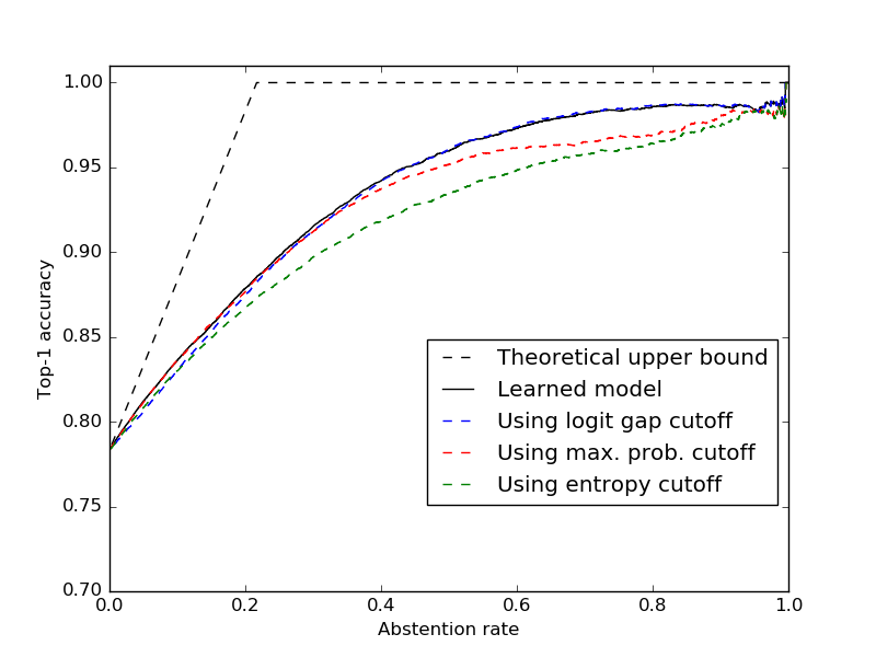
Figure 1: Accuracy vs. abstention rate for Inception v3.

Figure 1 illustrates the tradeoffs between accuracy and response rate that can be achieved by applying this rule to Inception-v3, measured on a second disjoint validation set of 25,000 images. The horizontal axis is the fraction of examples on which Inception-v3 returns $\bot$, and the vertical axis is top-1 accuracy on the remaining examples. For comparison, we also show for each feature the tradeoff curve obtained by simply thresholding the raw feature value. We also show the theoretically optimal tradeoff curve that would be achieved using an accuracy model that predicts top-1 accuracy perfectly (in which case we only return $\bot$ on examples Inception-v3 misclassifies).

Overall, Inception-v3 achieves 77% top-1 accuracy. However, if we set the logit gap cutoff threshold appropriately, we can achieve over 95% accuracy on the 44% of examples on which the model is most confident (while returning $\bot$ on the remaining 56%). Perhaps surprisingly, using the learned accuracy model gives a tradeoff curve almost identical to that obtained by simply thresholding the logit gap.

4.2 Cascades

Having shown the effectiveness of our abstention rules, we now evaluate our cascade-generation algorithm on a pool of state-of-the-art ImageNet classification models. Our pool consists of 23 models released as part of the TF-Slim library (Silberman & Guadarrama, 2016). The pool contains two recent NasNet models produced by neural architecture search (Zoph et al., 2017), five models based on the Inception architecture (Szegedy et al., 2016), and all 16 MobileNet models (Howard et al., 2017). We generate abstaining models by thresholding the logit gap value.

For each model $p$, and each $\alpha\in\left\{1-\frac{i}{100}:0\leq i\leq 5\right\}$, we used Algorithm 2 to generate a cascade with low cost, subject to the constraint that accuracy was at least $\alpha$ times that of $p$. We use number of multiplications as the cost.

When using Algorithm 2 it is important to use examples not seen during training, because statistics such as logit gap are distributed very differently for them. We used 25,000 images from the ILSVRC 2012 validation set (Russakovsky et al., 2015) to run the algorithm, and report results on the remaining 25,000 validation images.

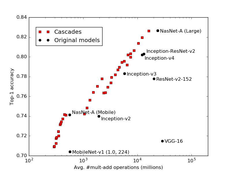
Figure 2: Cascades of pre-trained ImageNet models.

Figure 2 shows the tradeoffs we achieve between accuracy and average cost. Relative to the large (server-sized) NasNet model, we obtain a 1.5x reduction with no loss in accuracy. Relative to Inception-v4, one of the cascades obtains a 1.8x cost reduction with a no loss in accuracy, while another obtains a 1.2x cost reduction with a 1.2% increase in accuracy. Relative to the largest MobileNet model, we achieve a 2x cost reduction with a 0.5% accuracy gain.

We now examine the structure of an auto-generated cascade. Table 1 shows a cascade generated using a pool of 16 MobileNet models, with the most accurate MobileNet model as the reference model. The $i$th row of the table describes the (model, rule) pair used in the $i$th stage of the cascade. The cascade has several intuitive properties:

1. Earlier stages use cheaper models. Model used in earlier stages of the cascade have fewer parameters, use fewer multiplies, and have lower input image resolution.

2. Cheaper models require higher confidence. The minimum logit gap required to make a prediction is higher for earlier stages, reflecting the fact that cheaper models must be more confident in order to achieve sufficiently high accuracy.

3. Cheaper models handle easier images. Although overall model accuracy increases in later stages, accuracy on the subset of images actually classified by each stage is strictly decreasing (last column). This supports the idea that easier images are allocated to cheaper models.

4.3 Cascades of approximations

A large number of techniques have been developed for reducing the cost of deep neural networks via postprocessing. Such techniques include quantization, pruning of weights or channels, and tensor factorizations (see (Han et al., 2015) and references therein for further discussion). In this section, we show how these techniques can be used to generate a larger pool of approximated models, which can then be used as input to our cascade-generation algorithm in order to achieve further cost reductions. This also provides a way to make use of the cascade-generation algorithm in the case where only a single pre-trained model is available.

For these experiments, we focus on quantization of model parameters as the compression technique. For each model $m$, and each number of bits $b\in\{1,2,\ldots,16\}$, we generate a new model $m_{b}$ by quantizing all of $m$’s parameters to $b$ bits. This yields a pool of $23\cdot 16=368$ quantized models, which we use as input to the cascade-generation algorithm. Cost is the number of bits read from memory when classifying an example. Aside from these two changes, our experiments are identical to those in §4.2.

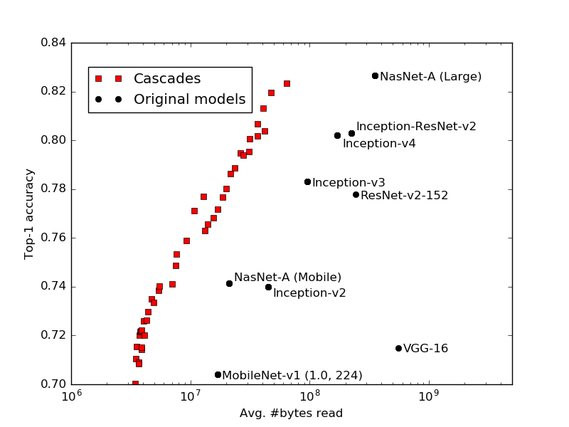
Figure 3: Cascades of quantized ImageNet models.

Figure 3 shows accuracy as a function of the average number of bits that must be fetched from memory in order to classify an example. Though the cascades generated in §4.2 (which were optimized for number of multiplications) do not consistently improve on average memory I/O, the cascades of approximations reduce it by up to a factor of 6 with no loss in accuracy. Perhaps surprisingly, the cascades of approximations also offer improvements in average-case number of multiplications similar to those shown in Figure 2, despite this not being an explicit component of the cost function.

5 Related work

The high-level goal of our work is to reduce average-case inference cost by spending less computation time on easier examples. This subject is the topic of a vast literature, with many distinct problem formulations spread across many domains.

Within the realm of computer vision, cascaded models received much attention following the seminal work of Viola and Jones (2001), who used a cascade of increasingly more expensive features to create a fast and accurate face detector. In problems such as speech recognition and machine translation, inference typically involves a heuristic search through the large space of possible outputs, and the cascade idea can be used to progressively filter the set of outputs under consideration (Weiss & Taskar, 2010).

Recent work has sought to apply the cascade idea to deep networks. Most research involves training an adaptive model end-to-end (Graves, 2016; Guan et al., 2017; Hu et al., 2017; Huang et al., 2017). Though end-to-end training is appealing, it is sensitive to the choice of model architecture. Current approaches for image classification are based on ResNet architectures, and do not achieve results competitive with the latest NasNet models on ImageNet.

Another way to produce adaptive deep networks is to apply postprocessing to a pool of pre-trained models, as we have done. To our knowledge, the only previous work that has taken this route is that of Bolukbasi et al. (2017), who also present results for ImageNet. In contrast to the greedy approximation algorithm presented in this work, their approach does not have good performance in the worst case, and also requires the pre-trained input models to be arranged into a directed acyclic graph a priori as opposed to learning this structure as part of the optimization process.

Finally, as already mentioned, our greedy approximation algorithm builds on previous greedy algorithms for min-sum set cover and related problems (Feige et al., 2004; Munagala et al., 2005; Streeter et al., 2007).

6 Conclusions

We presented a greedy meta-algorithm that can generate a cascaded model given a pool of pre-trained models as input, and proved that the algorithm has near-optimal worst-case performance under suitable assumptions. Experimentally, we showed that cascades generated using this algorithm significantly improve upon state-of-the-art ImageNet models in terms of both average-case number of multiplications and average-case memory I/O.

Our work leaves open several promising directions for future research. On the theoretical side, it remains an open problem to come up with more compelling theoretical guarantees for adaptive policies as opposed to linear cascades. Empirically, it would be very interesting to incorporate architecture search into the inner loop of the greedy algorithm, as discussed in §3.7.

References

- Bolukbasi et al. (2017) Bolukbasi, Tolga, Wang, Joseph, Dekel, Ofer, and Saligrama, Venkatesh. Adaptive neural networks for efficient inference. In Proceedings of the Thirty-fourth International Conference on Machine Learning, pp. 527–536, 2017.
- Feige et al. (2004) Feige, Uriel, Lovász, László, and Tetali, Prasad. Approximating min sum set cover. Algorithmica, 40(4):219–234, 2004.
- Golovin & Krause (2011) Golovin, Daniel and Krause, Andreas. Adaptive submodularity: Theory and applications in active learning and stochastic optimization. Journal of Artificial Intelligence Research, 42:427–486, 2011.
- Graves (2016) Graves, Alex. Adaptive computation time for recurrent neural networks. CoRR, abs/1603.08983, 2016.
- Guan et al. (2017) Guan, Jiaqi, Liu, Yang, Liu, Qiang, and Peng, Jian. Energy-efficient amortized inference with cascaded deep classifiers. CoRR, abs/1710.03368, 2017.
- Han et al. (2015) Han, Song, Mao, Huizi, and Dally, William J. Deep compression: Compressing deep neural networks with pruning, trained quantization and huffman coding. arXiv preprint arXiv:1510.00149, 2015.
- Howard et al. (2017) Howard, Andrew G., Zhu, Menglong, Chen, Bo, Kalenichenko, Dmitry, Wang, Weijun, Weyand, Tobias, Andreetto, Marco, and Adam, Hartwig. MobileNets: Efficient convolutional neural networks for mobile vision applications. CoRR, abs/1704.04861, 2017.
- Hu et al. (2017) Hu, Hanzhang, Dey, Debadeepta, Bagnell, J. Andrew, and Hebert, Martial. Anytime neural network: a versatile trade-off between computation and accuracy. CoRR, abs/1708.06832, 2017.
- Huang et al. (2017) Huang, Gao, Chen, Danlu, Li, Tianhong, Wu, Felix, van der Maaten, Laurens, and Weinberger, Kilian Q. Multi-scale dense networks for resource efficient image classification. CoRR, abs/1703.09844, 2017.
- Kuleshov & Liang (2015) Kuleshov, Volodymyr and Liang, Percy S. Calibrated structured prediction. In Advances in Neural Information Processing Systems, pp. 3474–3482, 2015.
- Munagala et al. (2005) Munagala, Kamesh, Babu, Shivnath, Motwani, Rajeev, Widom, Jennifer, and Thomas, Eiter. The pipelined set cover problem. In ICDT ’05: Proceedings of the 10th International Conference, volume 5, pp. 83–98. Springer, 2005.
- Russakovsky et al. (2015) Russakovsky, Olga, Deng, Jia, Su, Hao, Krause, Jonathan, Satheesh, Sanjeev, Ma, Sean, Huang, Zhiheng, Karpathy, Andrej, Khosla, Aditya, Bernstein, Michael, Berg, Alexander C., and Fei-Fei, Li. ImageNet Large Scale Visual Recognition Challenge. International Journal of Computer Vision (IJCV), 115(3):211–252, 2015. doi: 10.1007/s11263-015-0816-y.
- Silberman & Guadarrama (2016) Silberman, Nathan and Guadarrama, Sergio. Tf-slim: A high level library to define complex models in tensorflow. 2016. URL https://research.googleblog.com/2016/08/tf-slim-high-level-library-to-define.html.
- Streeter et al. (2007) Streeter, Matthew, Golovin, Daniel, and Smith, Stephen F. Combining multiple heuristics online. In Proceedings of the Twenty-second National Conference on Artificial Intelligence (AAAI’07), pp. 1197–1203, 2007.
- Szegedy et al. (2016) Szegedy, Christian, Vanhoucke, Vincent, Ioffe, Sergey, Shlens, Jon, and Wojna, Zbigniew. Rethinking the inception architecture for computer vision. In Proceedings of the IEEE Conference on Computer Vision and Pattern Recognition, pp. 2818–2826, 2016.
- Viola & Jones (2001) Viola, Paul and Jones, Michael. Rapid object detection using a boosted cascade of simple features. In CVPR, pp. 511–518, 2001.
- Weiss & Taskar (2010) Weiss, David and Taskar, Benjamin. Structured prediction cascades. In Proceedings of the Thirteenth International Conference on Artificial Intelligence and Statistics, pp. 916–923, 2010.
- Yuan & Wegkamp (2010) Yuan, Ming and Wegkamp, Marten. Classification methods with reject option based on convex risk minimization. Journal of Machine Learning Research, 11(Jan):111–130, 2010.
- Zoph et al. (2017) Zoph, Barret, Vasudevan, Vijay, Shlens, Jonathon, and Le, Quoc V. Learning transferable architectures for scalable image recognition. CoRR, abs/1707.07012, 2017.