The spatial Lambda-Fleming-Viot process with fluctuating selection

Abstract

We are interested in populations in which the fitness of different genetic types fluctuates in time and space, driven by temporal and spatial fluctuations in the environment. For simplicity, our population is assumed to be composed of just two genetic types. Short bursts of selection acting in opposing directions drive to maintain both types at intermediate frequencies, while the fluctuations due to ‘genetic drift’ work to eliminate variation in the population.

We consider first a population with no spatial structure, modelled by an adaptation of the Lambda (or generalised) Fleming-Viot process, and derive a stochastic differential equation as a scaling limit. This amounts to a limit result for a Lambda-Fleming-Viot process in a rapidly fluctuating random environment. We then extend to a population that is distributed across a spatial continuum, which we model through a modification of the spatial Lambda-Fleming-Viot process with selection. In this setting we show that the scaling limit is a stochastic partial differential equation. As is usual with spatially distributed populations, in dimensions greater than one, the ‘genetic drift’ disappears in the scaling limit, but here we retain some stochasticity due to the fluctuations in the environment, resulting in a stochastic p.d.e. driven by a noise that is white in time but coloured in space.

We discuss the (rather limited) situations under which there is a duality with a system of branching and annihilating particles. We also write down a system of equations that captures the frequency of descendants of particular subsets of the population and use this same idea of ‘tracers’, which we learned from Hallatschek and Nelson (2008) and Durrett and Fan (2016), in numerical experiments with a closely related model based on the classical Moran model.

Key words: Spatial Lambda Fleming-Viot model, Fluctuating selection, stochastic growth models, Tracer dynamics, scaling limits

MSC 2010 Subject Classification: Primary: 60G57, 60J25, 92D15
Secondary: 60J75, 60G55

1 Introduction

A fundamental challenge in population genetics is to understand the balance between adaptive processes (selection) and random neutral processes (genetic drift). The most studied example of adaptation is directional selection acting on a single genetic locus. In the simplest model, each individual is either of type $a$ or type $A$ at the locus under selection, and the relative fitnesses of individuals carrying the two types is $1+s_{0}:1$, for some small parameter $s_{0}$. At least provided that random fluctuations don’t eliminate the favoured type before it can become established, natural selection will act to remove variability from the population until, in the absence of mutation, everyone is of the favoured type. However, there are other forms of selection that act to maintain genetic variation. In this paper we are concerned with populations that are subject to changing environmental conditions, that cause relative fitnesses of different genotypes to fluctuate in time and space. To quote Gillespie (2004), “If fitnesses do depend on the state of the environment, as they surely must, then they must just as assuredly change in both time and space, driven by temporal and spatial fluctuations in the environment.”

We shall suppose that our population occurs in just two types (alleles), $\{a,A\}$ and that the environment fluctuates between two states, in the first of which $a$, and in the second of which $A$, is favoured. We suppose that selection is sufficiently strong that if the environment did not fluctuate, the favoured type would rapidly fix in the population, but that there is a ‘balance’ between the two environments so that both types can be maintained at non-trivial frequencies for long periods of time. If the population has no spatial structure, then over large timescales the frequency of $a$-alleles can be modelled by a stochastic differential equation:

$$\mathrm{d}p={\mathbf{s}}^{2}p(1-p)(1-2p)\mathrm{d}t+\sqrt{p(1-p)}\mathrm{d}B^{1}+\sqrt{2}{\mathbf{s}}p(1-p)\mathrm{d}B^{2},$$ (1.1)

where $B^{1}$ and $B^{2}$ are independent Brownian motions, the first (as we shall explain in Section 3) capturing the randomness due to genetic drift (that is the randomness due to reproduction in a finite population), the second encoding the random fluctuations in the environment (which are assumed to happen quickly on evolutionary timescales). The constant ${\mathbf{s}}$ is a scaled selection coefficient (see Section 3). For a population distributed across a one-dimensional spatial continuum, one can write down an analogous stochastic partial differential equation:

$$\mathrm{d}w(t,x)=\frac{1}{2}\Delta w(t,x)\mathrm{d}t+{\mathbf{s}}^{2}w(t,x)(1-w(t,x)(1-2w(t,x))\mathrm{d}t\\ +\sqrt{w(t,x)(1-w(t,x))}{\mathcal{W}}(\mathrm{d}t,\mathrm{d}x)+\sqrt{2}{\mathbf{s}}w(t,x)(1-w(t,x))W(\mathrm{d}t,\mathrm{d}x),$$ (1.2)

where ${\mathcal{W}}$ is space-time white noise (capturing genetic drift) and the independent noise $W$ is white in time, but may be coloured in space reflecting spatial correlations in the environmental fluctuations. In the biologically most relevant case of two dimensions, this equation has no solution, and we must find a different approach.

The difficulties with modelling genetic drift in populations evolving in higher dimensional spatial continua, often referred to as ‘the pain in the torus’, are well known; see Barton et al. (2013) for a review. They can be overcome using the spatial Lambda-Fleming-Viot process, introduced in Etheridge (2008) and rigorously constructed in, Barton et al. (2010), and here we adapt that model to incorporate fluctuating selection.

Our first result deals with the non-spatial case. We take a scaling limit of the Lambda-Fleming-Viot process and recover (1.1), which coincides with that obtained by Gillespie (2004) as a scaling limit of a Wright-Fisher type model. We then turn to the scaling limit of the spatial Lambda-Fleming-Viot process with fluctuating selection. In dimension one, the limiting process coincides (up to constants) with the stochastic p.d.e. (1.2). In higher dimensions, the term corresponding to genetic drift vanishes in the limit, but the effects of the fluctuations in the environment can still persist, resulting in a stochastic p.d.e. driven by (spatially) coloured noise.

Our ultimate aim is to find ways to distinguish the effects of spatial and temporal environmental fluctuations on genetic data. This would involve understanding the genealogical trees relating individuals in a sample from the population. Although for our prelimiting model we can write down an analogue of the ancestral selection graph of Krone and Neuhauser (1997), Neuhauser and Krone (1997), which tracks all ‘potential ancestors’ of individuals in a sample from the population, this process seems to be rather unwieldy. Moreover, when we apply our rescaling, the scaled ancestral selection graphs do not converge and we have not found a satisfactory way to extract genealogies for the limiting model. When selection does not fluctuate, the original ancestral selection graph can be thought of as a moment dual to the forwards in time diffusion describing allele frequencies in the population. It is natural to ask whether there are other dual processes that we could exploit when selection fluctuates. Our attempts to find a useful dual for the equation (1.2) have met with limited success, but in Section 5 we show that (after an affine transformation) there are circumstances in which a branching and annihilating dual exists.

In the absence of a useful dual process, instead we take a first step towards understanding ancestry in the population by following an interesting approach of Hallatschek and Nelson (2008) and, more recently, Durrett and Fan (2016) which uses the idea of ‘tracers’ to explore the way in which descendants of a subpopulation of the type $a$ individuals evolve forwards in time. In Section 6 we write down the system of stochastic p.d.e.’s that will determine the tracer dynamics. This idea is exploited further in our numerical experiments of Section 7.

The rest of the article is laid out as follows. In Section 2 we very briefly outline some of the biological background. In Section 3 we consider the case in which the population has no spatial structure. To prepare the ground for the case of spatially structured populations, we work with the Lambda-Fleming-Viot process (also sometimes known as the generalised Fleming-Viot process) that was introduced in Donnelly and Kurtz (1999), Bertoin and Le Gall (2003). In particular, we investigate different scaling limits, reflecting longtime behaviour of the process for different balances between the rate of changes of environment and the strength of selection. In Section 4 we define the spatial Lambda-Fleming-Viot process with fluctuating selection and give a precise statement of our scaling result for this model. In Section 5, we discuss the situations in which we can investigate the limiting process through duality with a system of branching and annihilating particles. Tracers are introduced in Section 6 and then explored numerically (for a Moran model of a subdivided population) in Section 7. The proof of our main scaling limit is in Section 8. The appendices contain some (important) technical results that we require in the course of the proofs.

Acknowledgement

We should like to thank Tom Kurtz and Amandine Véber for extremely helpful discussions and two anonymous referees for a careful reading of the manuscript and valuable suggestions.

2 Biological background

In this section we outline the biological context for this work. Although not a prerequisite for understanding the mathematics of subsequent sections, it explains our motivation for tackling this particular scaling limit.

Suppose that a gene occurs in just two forms that, because of environmental fluctuations, each finds itself subject to short alternating bursts of positive and negative selection. Even if these changes are happening on a much faster scale than neutral evolution, they may influence gene frequencies. For example, in diploid individuals (carrying two copies of the gene), a heterozygote (carrying one allele of each type) may have higher mean fitness, when we take account of different environments, than either homozygote, and so allelic variation can be maintained for long periods, even though at any given time the population is subject to directional selection. This marginal overdominance is an example of balancing selection. In equation (1.1) we see this in the deterministic term ($sp(1-p)(1-2p)\mathrm{d}t$) on the right hand side. 1969, Wright (1969) observed that spatial heterogeneity in the direction of selection combined with density dependent reproduction can also lead to balanced polymorphism, that is adaptive alleles are held at intermediate frequencies for long periods (see also Delph and Kelly (2014) and references therein).

One of the recurring arguments in evolutionary biology is whether evolution occurs principally through natural selection or through neutral processes, in which no particular genetic type is favoured, such as genetic drift. A data set that has sat at the heart of this debate for the last 70 years is a time series of changes in the genotype frequency of a polymorphism of the Scarlet Tiger Moth, Callimporpha (Panaxia) dominula, in an isolated population at Cothill Fen near Oxford, UK. Fisher and Ford (1947) found that the proportion of a certain medionigra allele in the population increased significantly between 1929 and 1941 from $1.2$% to $11.1$%, and decreased to $5.2$% between 1941 and 1946. They concluded, “$\ldots$ the observed fluctuations in generations are much greater than could be ascribed to random survival only. Fluctuations in natural selection must therefore be responsible for them.”. Fisher (a strong proponent of the importance of selection) was challenged by Wright (a champion of genetic drift) who argued that multiple factors could be at play and, moreover, Fisher may have underestimated the strength of genetic drift. (2005, O’Hara (2005) analysed the, by then 60 year long, time series of data from Cothill and concluded that most of the pattern of variation in the population should be attributed to genetic drift. Moreover, although selection is acting, mean fitness barely increased.

It is unusual to have such a long time series of data, especially in conjunction with information about the environment. In general it will also be far from clear which genes are undergoing selection, rather one tries to infer the action of selection through studying neutral diversity. For most populations, it may be very difficult to distinguish fluctuating selection from genetic drift. To see why, we recall a model due to Gillespie that captures the effect of a series of ‘selective sweeps’ through a population. Suppose that a selectively favoured mutation arises at some point on the genome and rapidly increases in frequency (until the whole population carries it). Because genes are arranged on chromosomes, different genes do not evolve independently of one another. As a result of a process called recombination, correlations between genes decrease as a function of the distance between them on the chromosome. Nonetheless, a neutral allele fortunate enough to be on the same chromosome as the selectively favoured mutation will itself receive a boost in its frequency (even if as a result of recombination it doesn’t exhaust the whole population). This boost to the type at the neutral locus is known as ‘genetic hitchhiking’, a term introduced by Maynard Smith and Haigh (1974). Of course, correspondingly, a neutral allele associated with an unfavoured type will decrease in frequency. Gillespie (2000), Gillespie (2001) investigated a model in which strongly selected mutations which give rise to hitchhiking events occur at the points of a Poisson process. He assumes that selection is strong enough that the duration of the sweeps causing the hitchhiking events that affect a given locus is small compared to the time between them so that we can ignore the possibility that a locus will be subject to two simultaneous hitchhiking events. He establishes that the first two moments of the change in allele frequency at the neutral locus over the course of a hitchhiking event take exactly the same form as if they had been produced by genetic drift over a single generation of reproduction. It is not hard to see that we will see the same hitchhiking effects under ‘partial sweeps’ driven by environmental fluctuations. This process of ‘genetic draft’ induced by selection, strongly resembles genetic drift and it may be hard to distinguish the two. Barton (2000) also considers the ‘genetic drift’ induced by hitchhiking.

Not surprisingly, the impact of environmental fluctuations on genetic variation has been extensively studied. Nonetheless, even in the absence of spatial structure, it remains an open question to characterise situations under which fluctuating environmental conditions can maintain genetic variation; see e.g. Novak and Barton (2017). Moreover, the effects of genetic drift have been largely ignored. This is perhaps because acting in isolation, genetic drift typically impacts gene frequencies over periods of (tens of) thousands of generations, much longer than the time scales of climatic fluctuation. However, once a particular genotype becomes rare, perhaps as a result of a run of unfavourable environments, stochastic fluctuations will be dominated by genetic drift, through which the genotype can be lost.

A further challenge in identifying genes that are subject to fluctuating selection is that, even if we can disentangle the effects of drift, numerous selection schemes lead to forms of balancing selection. For example, in the absence of spatial structure, allele frequency dynamics under fluctuating selection are identical to those under within-generation fecundity variance polymorphism. In this setting, Taylor (2013) shows that the effects on the genealogy at a linked neutral locus will differ. Fijarczyk and Babik (2015) and the references therein provide an overview of theoretical and empirical evidence for various forms of balancing selection and methods for their detection.

Recently, Bergland et al. (2014) reported hundreds of polymorphisms in Drosophila melanogaster whose frequencies oscillate among seasons and they attribute this to strong, temporally variable selection. They also cite evidence that genetic (and phenotypic) variation is maintained by temporally fluctuating selection for a variety of other organisms.Gompert (2016) proposes an approach to quantifying variable selection in populations experiencing both spatial and temporal variations in selection pressure. In spite of this combination of theoretical and empirical evidence for the importance of fluctuating selection, we have only a limited understanding of some basic questions: how many loci are subject to temporally fluctuating selection? How strong is that selection? What is the relationship between temporally and spatially varying selection?

Since natural environments are never truly constant, it is clearly important to understand the implication of temporally and spatially varying selection pressures. Cvijovic et al. (2015) examines some of the implications of temporal fluctuations. Our work here is a step towards a tractable framework in which to consider the combined effects of spatial and temporal fluctuations.

3 The non-spatial case

3.1 The (non-spatial) model

We first consider a population without spatial structure. Although we would obtain exactly the same scaling limits if we were to use the classical Moran or Wright-Fisher models as the basis of our approach, c.f. Gillespie (2004), for consistency with what follows, we shall work with the (non-spatial) Lambda-Fleming-Viot process. The key ideas that will be required in the spatial setting already appear here, where they are not obscured by notational complexity. An analogous scaling limit is obtained for the Wright-Fisher model with fluctuating selection (using similar reasoning) in Hutzenthaler et al. (2018).

We shall restrict ourselves to the special case of the Lambda-Fleming-Viot process in which reproduction events fall at a finite rate, determined by a Poisson process. We shall also suppose that there are just two types of individual, $\{a,A\}$. In each event, a parent is chosen from the population immediately before the event, and a portion $u$ of the population is replaced by offspring of the same type as the parent. In general the quantity $u$, which we shall call the impact of the event, may be random. Selection (on fecundity) can be incorporated by weighting the choice of parent, to favour one type or the other, and we shall extend previous versions of the model to allow the direction of selection to fluctuate. More precisely, we have the following definition.

Definition 3.1 (Lambda-Fleming-Viot process with fluctuating selection).

The Lambda-Fleming-Viot process with fluctuating selection, $\{p(t)\}_{t\geq 0}$ is a càdlàg process taking its values in $[0,1]$, with $p(t)$ to be interpreted as the proportion of type $a$ individuals in the population at time $t$.

Let $\Pi$ be a Poisson process defined on $\mathbb{R}\times(0,1)\times(0,1)$ with intensity measure $\mathrm{d}t\otimes\nu(\mathrm{d}u)\otimes\sigma(\mathrm{d}{\mathbf{s}})$, where $\nu$ and $\sigma$ are some probability measures. Moreover, let $\Pi^{env}$ be a rate $\tau^{env}$ Poisson process, independent of $\Pi$ (where $\tau^{env}\in(0,\infty))$. The state of the environment is a random variable $\zeta(t)\in\{-1,1\}$. At the times of the Poisson process $\Pi^{env}$, $\zeta$ is resampled uniformly from $\{-1,1\}$.

The dynamics of $\{p(t)\}_{t\geq 0}$ can be described as follows. If $(t,u,{\mathbf{s}})\in\Pi$, a reproduction event occurs. Then:

1. select a parental type $\kappa\in\{a,A\}$ according to

   $$\mathbb{P}[\kappa=a]=\frac{(1+{\mathbf{s}})p(t_{-})}{1+{\mathbf{s}}p(t_{-})}\quad\text{if}\quad\zeta=-1,$$

   $$\mathbb{P}[\kappa=a]=\frac{p(t_{-})}{1+{\mathbf{s}}(1-p(t_{-}))}\quad\text{if}\quad\zeta=1.$$

2. A proportion $u$ of the population immediately before the event dies and is replaced by offspring of the chosen type, that is

   $$p(t)=(1-u)p(t_{-})+\mathbf{1}_{\{\kappa=a\}}u.$$

Remark 3.2.

If, instead of resampling the environment according to an independent Poisson process, we resampled it at each reproduction event, by choosing $\nu$ to be distributed as the proportion of hitchhikers when a selective sweep occurs at a random distance from our chosen locus, we would recover Gillespie’s model of genetic draft at a neutral locus linked to loci undergoing a sequence of selective sweeps.

We shall see that the rate of resampling of the environment (relative to the strength of selection in each event) plays a key role in the long term behaviour of the population.

3.2 Scaling limits

In order to simplify the notation still further, we specialise to the case in which the Poisson point process $\Pi$ of Definition 3.1 has intensity $\mathrm{d}t\otimes\delta_{\bar{u}}\otimes\delta_{\mathbf{s}}$ for some fixed $\bar{u}$ and ${\mathbf{s}}$; in other words we fix the impact and the strength of selection in each event. A general result can be obtained from our calculations below by integration.

In order to obtain a diffusion approximation, we shall speed up the rate of reproduction events by a factor $n$, but scale down both the impact and the strength of the selection. We write $u_{n}$, ${\mathbf{s}}_{n}$ for the impact and strength of selection at the $n$th stage of our rescaling. We shall also scale $\Pi^{env}$ to have rate $n^{\gamma}$, with $\gamma>0$ to be chosen. We shall need the joint generator $\mathcal{L}^{(n)}$ of the pair $(p,\zeta)$ at the $n$th stage of this rescaling. We write $\pi$ for the uniform measure on $\{-1,1\}$ and $\mathbb{E}_{\pi}$ for the corresponding expectation. In an obvious notation, for suitable test functions $f$, we have

$$\mathcal{L}^{(n)}f(p,\zeta)=\mathbf{1}_{\{\zeta=-1\}}n\left(\left[\frac{(1+{\mathbf{s}}_{n})p}{1+{\mathbf{s}}_{n}p}\right]f\left((1-u_{n})p+u_{n},\zeta\right)\right.\\ \left.\phantom{blablablablablablablablablabla}+\left[\frac{1-p}{1+{\mathbf{s}}_{n}p}\right]f\left((1-u_{n})p,\zeta\right)-f(p,\zeta)\right)\\ +\mathbf{1}_{\{\zeta=1\}}n\left(\left[\frac{p}{1+{\mathbf{s}}_{n}(1-p)}\right]f\left((1-u_{n})p+u_{n},\zeta\right)\right.\\ \left.\phantom{blablablablablablablablablabla}+\left[\frac{(1+{\mathbf{s}}_{n})(1-p)}{1+{\mathbf{s}}_{n}(1-p)}\right]f\left((1-u_{n})p,\zeta\right)-f(p,\zeta)\right)\\ +n^{\gamma}\left(\mathbb{E}_{\pi}[f(p,\cdot)]-f(p,\zeta)\right).$$

Expanding the ratios involving ${\mathbf{s}}_{n}$ as geometric series, and using Taylor’s Theorem to expand $f$ (as a function of $p$), we obtain

$$\mathcal{L}^{(n)}f(p,\zeta) =n\{p-{\mathbf{s}}_{n}\zeta p(1-p)+\mathcal{O}({\mathbf{s}}_{n}^{2})\}$$

$$\qquad\qquad\times\{u_{n}(1-p)f^{\prime}(p,\zeta)+\frac{1}{2}u_{n}^{2}(1-p)^{2}f^{\prime\prime}(p,\zeta)+\mathcal{O}(u_{n}^{3})\}$$

$$+n\{(1-p)+{\mathbf{s}}_{n}\zeta p(1-p)+\mathcal{O}({\mathbf{s}}_{n}^{2})\}$$

$$\qquad\qquad\times\{-u_{n}pf^{\prime}(p,\zeta)+\frac{1}{2}u_{n}^{2}p^{2}f^{\prime\prime}(p,\zeta)+\mathcal{O}(u_{n}^{3})\}$$

$$+n^{\gamma}\left(\mathbb{E}_{\pi}[f(p,\cdot)]-f(p,\zeta)\right)$$

$$= \frac{1}{2}nu_{n}^{2}p(1-p)f^{\prime\prime}(p,\zeta)-n{\mathbf{s}}_{n}u_{n}\zeta p(1-p)f^{\prime}(p,\zeta)$$

$$+n^{\gamma}\left(\mathbb{E}_{\pi}[f(p,\zeta)]-f(p,\zeta)\right)+\mathcal{O}\left(n({\mathbf{s}}_{n}^{2}u_{n}+u_{n}^{2}{\mathbf{s}}_{n}+u_{n}^{3})\right).$$ (3.1)

In order to obtain a diffusion limit, we see that we should take $nu_{n}^{2}$ to be $\mathcal{O}(1)$. If the environment didn’t change, then we would require $nu_{n}{\mathbf{s}}_{n}$ to be $\mathcal{O}(1)$ and on passage to the limit recover the classical Wright-Fisher diffusion with selection, whose generator, if $\zeta=-1$ say, takes the form

$$\mathcal{L}^{WFS}f(p)=\frac{1}{2}p(1-p)f^{\prime\prime}(p)+{\mathbf{s}}p(1-p)f^{\prime}(p).$$

Since we are modelling short bursts of strong selection, we set

$$u_{n}=n^{-\frac{1}{2}}\bar{u}\quad{\mathbf{s}}_{n}=n^{-\frac{1}{2}+\alpha}{\mathbf{s}},$$ (3.2)

for some $\alpha\in(0,1/4)$. The restriction $\alpha<1/4$ ensures that the error term $n{\mathbf{s}}_{n}^{2}u_{n}$ in the expression (3.2) is negligible as $n\to\infty$.

We can then write the rescaled generator in the form

$$\mathcal{L}^{(n)}f(p,\zeta)=\mathcal{L}^{neu}f(p,\zeta)+n^{\alpha}\mathcal{L}^{fsel}f(p,\zeta)+n^{\gamma}\mathcal{L}^{env}f(p,\zeta)+\mathcal{O}\left(n^{-\frac{1}{2}+2\alpha}\right),$$ (3.3)

where

$$\mathcal{L}^{neu}f(p,\zeta) =\frac{1}{2}\bar{u}^{2}p(1-p)f^{\prime\prime}(p,\zeta)$$

$$\mathcal{L}^{fsel}f(p,\zeta) =-\zeta\bar{u}{\mathbf{s}}p(1-p)f^{\prime}(p,\zeta)$$

$$\mathcal{L}^{env}f(p,\zeta) =\mathbb{E}_{\pi}[f(p,\zeta)]-f(p,\zeta).$$

To see how we should choose $\gamma$, we employ a ‘separation of timescales’ trick due to Kurtz (1973). We apply the generator (3.3) to test functions of the form

$$g(p,\zeta)=f(p)+n^{-\delta}\left(\mathcal{L}^{fsel}f\right)(p,\zeta).$$ (3.4)

For this choice, we obtain

$$\mathcal{L}g(p,\zeta)=\mathcal{L}^{neu}f(p)+n^{\alpha}\left(\mathcal{L}^{fsel}f\right)(p,\zeta)+n^{-\delta}\mathcal{L}^{neu}\left(\mathcal{L}^{fsel}_{n}f\right)(p,\zeta)\\ +n^{\alpha-\delta}\mathcal{L}^{fsel}\left(\mathcal{L}^{fsel}f\right)(p,\zeta)-n^{\gamma-\delta}\left(\mathcal{L}^{fsel}f\right)(p,\zeta)+\mathcal{O}\left(n^{-\frac{1}{2}+2\alpha}\right),$$ (3.5)

where we have used the fact that $\mathcal{L}^{env}f(p)=0$ (since $f$ does not depend on $\zeta$) and $\mathbb{E}_{\pi}[n^{-\delta}\left(\mathcal{L}^{fsel}f\right)(p,\zeta)]=0$, since $\mathbb{E}_{\pi}[\zeta]=0$.

Evidently, to obtain a non-trivial limit we should take $\gamma=\delta+\alpha$. The most interesting case is when $\delta=\alpha$ and so $\gamma=2\alpha$. In that case, letting $n\to\infty$, in the limit the equation (3.5) becomes

$$\mathcal{L}f(p,\zeta)=\mathcal{L}^{neu}f(p)+\mathcal{L}^{fsel}\left(\mathcal{L}^{fsel}f\right)(p,\zeta).$$ (3.6)

To evaluate the right hand side,

$$\mathcal{L}^{fsel}\left(\mathcal{L}^{fsel}f\right)(p,\zeta) =\mathcal{L}^{fsel}\left(-\zeta\bar{u}{\mathbf{s}}p(1-p)f^{\prime}(p)\right)=\zeta^{2}\bar{u}^{2}{\mathbf{s}}^{2}p(1-p)\frac{d}{dp}\left(p(1-p)\frac{d}{dp}f(p)\right)$$

$$=\zeta^{2}\bar{u}^{2}{\mathbf{s}}^{2}p(1-p)(1-2p)f^{\prime}(p)+\zeta^{2}\bar{u}^{2}{\mathbf{s}}^{2}p^{2}(1-p)^{2}f^{\prime\prime}(p).$$

Noting that $\zeta^{2}\equiv 1$, equation (3.6) then reads

$$\mathcal{L}f(p)=\bar{u}^{2}{\mathbf{s}}^{2}p(1-p)(1-2p)f^{\prime}(p)+\left(\frac{1}{2}\bar{u}^{2}p(1-p)+\bar{u}^{2}{\mathbf{s}}^{2}p^{2}(1-p)^{2}\right)f^{\prime\prime}(p).$$

Remark 3.3.

There are other limits that can be obtained when $\gamma>2\alpha$. For example if $\alpha=1/4$ and we resample the environment at every reproduction event, corresponding to $\gamma>1$, then Miller (2012) shows that, under the same scaling of $u_{n}$, the frequency of type $a$ alleles in the population converges weakly to the solution of

$$\mathrm{d}p=\frac{1}{2}{\mathbf{s}}^{2}\bar{u}p(1-p)(1-2p)\mathrm{d}t+\bar{u}\sqrt{p(1-p)}\mathrm{d}B_{t}$$

for a standard Brownian motion $\{B_{t}\}_{t\geq 0}$. The deterministic drift here arises from the term of order $nu_{n}{\mathbf{s}}_{n}^{2}$ that under our previous scaling we were able to neglect in (3.2).

Based on these calculations, the following proposition follows easily from Theorem 2.1 of Kurtz (1992), which we recall later as Theorem 8.1. In the interests of space, we omit the details of the proof, which follows from exactly the same arguments as those that we employ in the spatial setting.

Proposition 3.4.

Let $\{p^{(n)}(t)\}_{t\geq 0}$ denote the (non-spatial) Lambda-Fleming-Viot process of Definition 3.1 in which $\Pi$ has intensity $n\mathrm{d}t\otimes\delta{u_{n}}\otimes\delta_{\mathbf{s}_{n}}$, where

$$u_{n}=n^{-1/2}\bar{u},\quad{\mathbf{s}}_{n}=n^{-1/2+\alpha}{\mathbf{s}},\mbox{ and }\tau^{env}=n^{2\alpha},$$

for some $\alpha\in(0,1/4)$. Suppose further that the sequence of initial conditions $\{p^{(n)}(0)\}_{n\geq 1}$ converges to $p_{0}$ as $n\to\infty$. Then as $n$ tends to infinity, $\{p^{(n)}(t)\}_{t\geq 0}$ converges weakly in $\mathcal{D}([0,\infty),[0,1])$ (the space of càdalàg functions taking values in $[0,1]$) to the one-dimensional diffusion with drift

$$\bar{u}^{2}{\mathbf{s}}^{2}p(1-p)(1-2p)$$

and quadratic variation

$$\bar{u}^{2}p(1-p)+2\bar{u}^{2}{\mathbf{s}}^{2}p^{2}(1-p)^{2},$$

started from $p_{0}$. In other words, the limiting process is the unique weak solution to the equation

$$\mathrm{d}p(t)=\bar{u}^{2}{\mathbf{s}}^{2}p(t)(1-p(t))(1-2p(t))\mathrm{d}t\\ +\bar{u}\sqrt{p(t)(1-p(t))}\mathrm{d}B_{t}^{1}+\sqrt{2}\bar{u}{\mathbf{s}}p(t)(1-p(t))\mathrm{d}B_{t}^{2},$$ (3.7)

with $p(0)=p_{0}$, and $\{B^{1}_{t}\}_{t\geq 0}$, $\{B_{t}^{2}\}_{t\geq 0}$ independent standard Brownian Motions.

4 Definition and scaling of the SLFVFS

In this section we first extend the Lambda-Fleming-Viot model with fluctuating selection of Section 3 to the spatial setting. The idea is simple: reproduction events are still driven by a Poisson point process, but now, in addition to specifying the strength of selection and the impact associated with each event, we must also specify the spatial region in which it takes place. As has become usual in this framework, we shall take those regions to be closed balls (indeed for simplicity we shall take our events to be of a fixed radius), but the same results will hold under much more general conditions, subject to some symmetry and boundedness assumptions. Having defined the model, we state our main scaling result for the spatial model.

4.1 Spatial Lambda-Fleming-Viot process with fluctuating selection

We suppose that the population, which is distributed across $\mathbb{R}^{d}$, is subdivided into two genetic types $\{a,A\}$. As explained in detail in Etheridge et al. (2018), which in turn borrows results from Véber and Wakolbinger (2015), formally, at each time the state of the population is described by a measure $M_{t}$ on $\mathbb{R}^{d}\times K$, where $K=\{a,A\}$, whose first marginal is Lebesgue measure on $\mathbb{R}^{d}$. This space of measures, which we denote by ${\cal M}_{\lambda}$, is equipped with the topology of vague convergence, under which it is compact. At any fixed time there is a density $w(t,\cdot):\mathbb{R}^{d}\rightarrow[0,1]$ such that

$$M_{t}(dx,d\kappa)=\left(w(t,x)\delta_{a}(d\kappa)+(1-w(t,x))\delta_{A}(d\kappa)\right)\mathrm{d}x.$$

Of course $w(t,x)$, which one should interpret as the proportion of the population at the location $x$ at time $t$ that is of type $a$, is only defined up to a Lebesgue null set. In what follows, we shall consider a representative of the density of $M_{t}$. It will be convenient to fix a representative $w(0,\cdot)$ of $M_{0}$ and then update it using the procedure described in the definition below, but the reader should bear in mind that the fundamental object is the measure-valued evolution. This becomes important when we talk about convergence of our rescaled processes; tightness will be immediate in the space of measures, but we will need to work harder to identify the dynamics of the density of the limit.

In what follows, for every $f\in C_{c}$ (continuous functions of compact support on $\mathbb{R}^{d}$) we shall use the notation

$$\left\langle w,f\right\rangle=\int_{\mathbb{R}^{d}}w(x)f(x)\mathrm{d}x.$$

Recall that the limit that we obtained in Section 3 corresponded to our throwing away the terms of order $n{\mathbf{s}}_{n}^{2}u_{n}$ in (3.2). In other words we approximated $(1+{\mathbf{s}})p/(1+{\mathbf{s}}p)$ by $p+{\mathbf{s}}p(1-p)=p(1-{\mathbf{s}})+{\mathbf{s}}\left(1-(1-p)^{2}\right)$ and similarly $p/(1+{\mathbf{s}}(1-p))$ was approximated by $p-{\mathbf{s}}p(1-p)=p(1-{\mathbf{s}})+{\mathbf{s}}p^{2}$. Under this approximation, since reproduction events are based on a Poisson process of events, we can think of splitting those events into two types: neutral events and selective events. In the non-spatial setting, neutral events occur at rate $(1-{\mathbf{s}})$ and, for such an event, the chance that the parent is type $a$ is $p$. Selective events fall at rate ${\mathbf{s}}$. One then selects two ‘potential’ parents. If $\zeta=-1$, then the offspring are type $a$ provided not both potential parents are type $A$, which has probability $1-(1-p)^{2}$, whereas if $\zeta=1$, the offspring are type $a$ only if both potential parents are type $a$ (probability $p^{2}$).

To avoid additional algebra, we shall define the spatial version of our model using this approximation. In our main scaling result, we shall indeed choose our scaling in such a way that $n{\mathbf{s}}_{n}^{2}u_{n}\to 0$ as $n\to\infty$.

Definition 4.1 (Spatial Lambda-Fleming-Viot process with fluctuating selection (SLFVFS)).

Let $\mu$ be a measure on $(0,\infty)$ and for each $r\in(0,\infty)$, let $\nu_{r}$ be a probability measure on $[0,1]$, such that the mapping $r\rightarrow\nu_{r}$ is measurable and

$$\int_{(0,\infty)}r^{d}\int_{[0,1]}u\;\nu_{r}(\mathrm{d}u)\mu(\mathrm{d}r)<\infty.$$ (4.1)

Further, fix ${\mathbf{s}}\in[0,1]$ and let $\Pi^{neu}$, $\Pi^{fsel}$, be independent Poisson point processes on $\mathbb{R}_{+}\times\mathbb{R}^{d}\times(0,\infty)\times[0,1]$ with intensity measures $(1-{\mathbf{s}})\mathrm{d}t\otimes\mathrm{d}x\otimes\mu(\mathrm{d}r)\nu_{r}(\mathrm{d}u)$ and ${\mathbf{s}}\mathrm{d}t\otimes\mathrm{d}x\otimes\mu(\mathrm{d}r)\nu_{r}(\mathrm{d}u)$ respectively.

Let $\Pi^{env}$ be a Poisson process, independent of $\Pi^{neu}$, $\Pi^{fsel}$, with intensity $\tau^{env}$, dictating the times of the changes in the environment. Let $\{\xi^{(m)}(\cdot)\}_{m\geq 0}$ be a family of identically distributed random fields such that

$$\mathbb{P}\left[\xi^{(m)}(x)=-1\right]=\frac{1}{2}=\mathbb{P}\left[\xi^{(m)}(x)=+1\right],$$

$$\mathbb{E}\left[\xi^{(m)}(x)\xi^{(m)}(y)\right]=g(x,y),$$

where the covariance function $g(x,y)$ is an element of $C_{b}\left(\mathbb{R}^{d}\times\mathbb{R}^{d}\right)$. Set $\tau_{0}=0$ and write $\{\tau_{m}\}_{m\geq 1}$ for the points in $\Pi^{env}$ and define

$$\zeta(t,\cdot):=\sum_{m=0}^{\infty}\xi^{(m)}(\cdot)\mathbf{1}_{[\tau_{m},\tau_{m+1})}(t).$$

In other words, the environment $\zeta(t,\cdot)$ is resampled, independently, at the times of the Poisson process $\Pi^{env}$.

The spatial Lambda-Fleming-Viot process with fluctuating selection (SLFVFS) with driving noises $\Pi^{neu}$, $\Pi^{fsel}$, $\Pi^{env}$, is the $\mathcal{M}_{\lambda}$-valued process $M_{t}$ with dynamics described as follows. Let $w(t_{-},\cdot)$ be a representative of the density of $M_{t_{-}}$ immediately before an event $(t,x,r,u)$ from $\Pi^{neu}$ or $\Pi^{fsel}$. Then the measure $M_{t_{-}}$ immediately after the event has density $w(t,\cdot)$ determined by:

1. If $(t,x,r,u)\in\Pi^{neu}$, a neutral event occurs at time $t$ within the closed ball $B(x,r)$. Then

   1. Choose a parental location $l$ according to the uniform distribution on $B(x,r)$.

   2. Choose the parental type $\kappa\in\{a,A\}$ according to the distribution

      $$\mathbb{P}\left[\kappa=a\right]=w(t_{-},l),\quad\mathbb{P}\left[\kappa=A\right]=1-w(t_{-},l).$$

   3. A proportion $u$ of the population within $B(x,r)$ dies and is replaced by offspring with type $\kappa$. Therefore, for each point $y\in B(x,r)$,

      $$w(t,y)=w(t_{-},y)(1-u)+u\mathbf{1}_{\{\kappa=a\}}.$$

2. If $(t,x,r,u)\in\Pi^{fsel}$, a selective event occurs at time $t$ within the closed ball $B(x,r)$. Then

   1. Choose two parental locations $l_{0},l_{1}$ independently, according to the uniform distribution on $B(x,r)$.

   2. Choose the two parental types, $\kappa_{0},\kappa_{1},$ independently, according to

      $$\mathbb{P}\left[\kappa_{i}=a\right]=w(t_{-},l_{i}),\quad\mathbb{P}\left[\kappa_{i}=A\right]=1-w(t_{-},l_{i}).$$

   3. A proportion $u$ of the population within $B(x,r)$ dies and is replaced by offspring with type chosen as follows:

      1. If $\zeta(t,x)=1$, their type is set to be $a$ if $\kappa_{0}=\kappa_{1}=a$, and $A$ otherwise. Thus for each $y\in B(x,r)$

         $$w(t,y) =(1-u)w(t_{-},y)+u\mathbf{1}_{\{\kappa_{0}=\kappa_{1}=a\}}.$$

      2. If $\zeta(t,x)=-1$, their type is set to be $a$ if $\kappa_{0}=\kappa_{1}=a$ or $\kappa_{0}\neq\kappa_{1}$ and $A$ otherwise, so that for each $y\in B(x,r)$,

         $$w(t,y) =(1-u)w(t_{-},y)+u\left(\mathbf{1}_{\{\kappa_{0}=\kappa_{1}=a\}}+\mathbf{1}_{\{\kappa_{0}\neq\kappa_{1}\}}\right).$$

We have tacitly assumed that $w(t_{-},l_{i})$ is defined. It is, with probability one, so we declare that if it is not defined, then we resample and try again. For a construction of the random fields $\{\xi^{(m)}(\cdot)\}_{m\geq 0}$ of Definition 4.1 we refer to Ma (2009), especially their Example 1. The arguments presented there require only minor adaptation.

Existence of the SLFVFS is guaranteed by the methods of Etheridge et al. (2018). Indeed, we could have taken different measures $\mu$ and $\nu_{r}$ according to whether events are selective or neutral. Although it is convenient to take the strength of selection to be constant in space and have its direction determined by the variable $\zeta\in\{-1,+1\}$, we could, of course, have defined a much more general model. For example, one could allow ${\mathbf{s}}$ to vary in space, or even resample ${\mathbf{s}}\zeta$ from a suitable random field whenever the environment is resampled. However, this would be at the expense of considerably more complicated notation and it would become more involved to exploit the Poisson structure of our model. See Remark 4.4 below for some comments on when our scaling result would generalise.

One of the key tools in the study of the neutral SLFV is the dual process of coalescing random walkers which traces out the genealogical trees relating individuals in a sample from the population. An ancestral lineage doesn’t move until it is both in the region affected by an event and is among the offspring of that event, at which time it jumps to the location of the parent of the event (which is uniformly distributed on the affected region). Things are more complicated in the presence of selection. Whereas in the neutral case we can always identify the distribution of the location of the parent of each event, now, at a selective event, even knowing the state of the environment, we are unable to identify which of the ‘potential parents’ is the true parent of the event without knowing their types. These can only be established by tracing further into the past. The resolution is to follow all potential ancestral lineages backwards in time. This results in a system of branching and coalescing walks in which branching and coalescence events are ‘marked’ according to the state of the environment at the time at which they occur.

Just as in the neutral case, the dynamics of the dual are driven by the time reversals $\overleftarrow{\Pi}^{neu}$, $\overleftarrow{\Pi}^{sel}$, $\overleftarrow{\Pi}^{env}$ of the Poisson point processes of events that drove the forwards in time process, that is

$$\overleftarrow{\Pi}^{i}:=\left\{(-t,x,r,u):(t,x,r,u)\in\Pi^{i}\right\},\quad i\in\{\text{neu},\text{sel},\text{env}\}.$$

The distribution of these Poisson point processes is invariant under the time reversal.

We emphasize that time for the process of ancestral lineages runs in the opposite direction to that for the allele frequencies. Our dual will relate the distribution of allele frequencies in a sample from the population at a time $T$, to allele frequencies at time $0$. More precisely, suppose that we know the frequencies $w(0,\cdot)$ of $a$-alleles at time $0$. At time $T$, which we think of as ‘the present’, we sample $j$ individuals from locations $\chi_{0}^{1},\ldots,\chi_{0}^{j}$. Tracing backwards in time, we write $\chi_{s}^{1},\ldots,\chi_{s}^{N_{s}}$ for the locations of the $N_{s}$ potential ancestors that make up our dual at time $s$ before the present.

Definition 4.2 (Ancestral selection graph).

We first define a $\bigcup_{n\geq 1}(\mathbb{R}^{d})^{n}$-valued Markov process, $((\chi^{i}_{t})_{i=1}^{N_{t}})_{t\geq 0}$, enriched by ‘environmental marks’ as follows:

At each $\tau\in\overleftarrow{\Pi}^{env}$ the environment is resampled;

At each event $(t,x,r,u)\in\overleftarrow{\Pi}^{neu}$,

1. for each $\chi_{t_{-}}^{i}\in B(x,r)$, independently mark the corresponding potential ancestor with probability $u$;

2. if at least one lineage is marked, all marked lineages disappear and are replaced by a single potential ancestor, whose location is drawn uniformly at random from within $B(x,r)$.

At each event $(t,x,r,u)\in\overleftarrow{\Pi}^{sel}$:

1. for each $\chi_{t_{-}}^{i}\in B(x,r)$, independently mark the corresponding potential ancestor with probability $u$;

2. if at least one lineage is marked, all marked lineages disappear and are replaced by two potential ancestors, whose locations are drawn independently and uniformly from within $B(x,r)$. The type of the environment is recorded.

In both cases, if no particles are marked, then nothing happens.

To determine the distribution of types of a sample of the population $w(T,\cdot)$, taken from locations $\chi_{0}^{1},\ldots,\chi_{0}^{j}$, knowing the distribution of $w(0,\cdot)$ at time $T$ before the present, first evolve the process of branching and coalescing lineages until time $T$. At time $T$ assign types to $\chi_{T}^{1},\ldots,\chi_{T}^{N_{T}}$ using independent Bernoulli random variables such that $\mathbb{P}[\mathtt{Type}(\chi_{T}^{i})=a]=w(0,\chi_{T}^{i})$. Tracing back through the system of branching and coalescing lineages $(\chi^{i}_{t})_{i=1}^{N_{t}}$, we define types recursively: at each neutral event the lineages that coalesced during the event are assigned the type of the parent; at a selective event, if $Z=1$ then all coalescing lineages are type $a$ if and only if both parents are type $a$, otherwise they are type $A$ whereas if $Z=-1$, all coalescing lineages are type $A$ if and only if both parents are type $A$, otherwise they are type $a$. The distribution of types at time zero is the desired quantity.

Since we only consider finitely many initial individuals in the sample, the jump rate in this process is finite and so this description gives rise to a well-defined process.

This dual process is the analogue for the SLFVFS of the Ancestral Selection Graph (ASG), introduced in the companion papersKrone and Neuhauser (1997), Neuhauser and Krone (1997), which describes all the potential ancestors of a sample from a population evolving according to the Wright-Fisher diffusion with selection. Indeed we could be more careful and use this process to extract the genealogy of a sample from the population. However, in this setting, this object seems to be rather unwieldy and, under the scalings in which we are interested, it will not converge to a well-defined limit.

Remark 4.3.

Informally, the procedure described above allows us to write down an expression, in terms of the marked process of branching and coalescing ancestral lineages and $w(0,\cdot)$, for $\mathbb{E}[\prod_{i=1}^{j}w(T,\chi_{0}^{i})]$; that is the probability that $j$ individuals, sampled from the present day population at locations $\chi_{0}^{1},\ldots,\chi_{0}^{j}$, are all of type $a$. More formally, since the density of the SLFVFS is only defined Lebesgue-almost everywhere, the quantities $w(T,\chi_{0}^{i})$ are only defined for Lebesgue almost every choice of $\chi_{0}^{1},\ldots,\chi_{0}^{j}$ and, just as in Etheridge et al. (2018) Section 1.2, this duality must be defined ‘weakly’, that is by integrating against a suitable test function $\psi(\chi_{0}^{1},\ldots,\chi_{0}^{j})$. Also mirroring that setting, the resulting ‘moment duality’ is sufficient to guarantee uniqueness of the SLFVFS. Since we do not use the duality in what follows, we refer the reader to Etheridge et al. (2018) for details.

4.2 Scaling the SLFVFS

We are interested in the effects of fluctuating selection over large spatial and temporal scales and so we shall consider a rescaling of our model. Etheridge et al. (2018) consider the corresponding process in which selection does not fluctuate with time, but instead always favours type $A$ (say). In that setting it is shown that if impact scales as $u_{n}=\bar{u}/n^{1/3}$ and selection scales as ${\mathbf{s}}_{n}={\mathbf{s}}/n^{2/3}$, then as $n\to\infty$, $w(nt,n^{1/3}x)$ (or rather a local average of this quantity) converges in $d\geq 2$ to the solution to the deterministic Fisher-KPP equation, and to the solution of the corresponding stochastic p.d.e. in which a ‘Wright-Fisher noise’ term, corresponding to genetic drift, has been added in $d=1$. Here we wish to consider short periods of stronger selection and so, by analogy with what we did in Section 3, we choose ${\mathbf{s}}_{n}={\mathbf{s}}n^{\alpha}/n^{2/3}$ for some $\alpha>0$, but we change the favoured type at times of mean $1/n^{2\alpha}$. This is of course the scaling suggested by the Central Limit Theorem (and is the natural analogue of our results in Section 3). In order to be able to ignore terms of order $n{\mathbf{s}}_{n}^{2}u_{n}$, we must now take $\alpha\in(0,1/6)$.

We must also scale the environment in a consistent way. In the examples that we have in mind, environmental correlations can be expected to extend over very large scales and so we actually fix the correlations in the limiting environment by fixing the distribution of a random field $\xi$ and at the $n$th stage of the scaling sampling the environment according to $\xi_{n}$ determined by

$$\xi(x)=\xi_{n}(n^{-\frac{1}{3}}x).$$

At the $n$th stage of the rescaling, the environment will be resampled at points of a rate $n^{2\alpha}$ Poisson process.

Remark 4.4 (Extensions).

We have taken selection to be constant in magnitude and just to vary in sign. This is not necessary, even for our scaling result. As an obvious extension, we could fix the distribution of ${\mathbf{s}}(x)\xi(x)$ and, at the $n$th stage of the scaling define

$${\mathbf{s}}_{n}(n^{-1/3}x)\xi_{n}(n^{-1/3}x)=\frac{n^{\alpha}}{n^{2/3}}\mathbf{s}(x)\xi(x),$$

At the expense of introducing an additional truncation of $\mathbf{s}(x)$ at the $n$th stage, to ensure that the $|\mathbf{s}_{n}(x)\xi_{n}(x)|<1$, it is enough to insist that

$$\mathbb{P}[\mathbf{s}(x)\xi(x)>z]=\mathbb{P}[\mathbf{s}(x)\xi(x)<-z],\quad\forall z\in\mathbb{R},$$

and

$$\mathbb{E}[|\mathbf{s}(x)\xi(x)|^{2+\epsilon}]<\infty,\qquad\mbox{for some }\epsilon>0,$$

plus some regularity to reflect equation (4.3) below. To avoid a proliferation of notation, we omit this somewhat artificial generalisation of our results.

Our definition of the SLFVFS is still rather general. We include it to underline the possibility of extending our results. However, in the interest of avoiding even more complex expressions than those that follow, from now on we shall specialise to fix the radius and impact of reproduction events.

Assumption 4.5.

From now on, fix $R\in(0,\infty)$ and $\bar{u}\in(0,1)$ and take

$$\mu({dr})=\delta_{R}(\mathrm{d}r),\qquad\nu_{r}(\mathrm{d}u)=\delta_{\bar{u}}(\mathrm{d}u).$$

Just as in Etheridge et al. (2018), we shall prove convergence, not of the sequence of densities of the SLFVFS, but of a sequence of local averages. We require some notation. Let $R$ be the fixed radius of events. Set

$$R_{n}=n^{-\frac{1}{3}}R,\quad B_{n}(x)=B(x,R_{n}),$$

and define the sequence of rescaled processes

$$w_{n}(t,x)=w(nt,n^{\frac{1}{3}}x),\quad\overline{w}_{n}(t,x)=\mathchoice{\mathop{\kern 1.99997pt\vrule width=6.00006pt,height=3.0pt,depth=-2.49997pt\kern-8.00003pt\intop}\nolimits_{\kern-2.79996ptB_{n}(x)}}{\mathop{\kern 1.00006pt\vrule width=5.0pt,height=3.0pt,depth=-2.59996pt\kern-6.00006pt\intop}\nolimits_{B_{n}(x)}}{\mathop{\kern 1.00006pt\vrule width=5.0pt,height=3.0pt,depth=-2.59996pt\kern-6.00006pt\intop}\nolimits_{B_{n}(x)}}{\mathop{\kern 1.00006pt\vrule width=5.0pt,height=3.0pt,depth=-2.59996pt\kern-6.00006pt\intop}\nolimits_{B_{n}(x)}}w_{n}(t,y)\mathrm{d}y,$$ (4.2)

where $\mathchoice{\mathop{\kern 1.99997pt\vrule width=6.00006pt,height=3.0pt,depth=-2.49997pt\kern-8.00003pt\intop}\nolimits_{\kern-2.79996ptB_{n}(x)}}{\mathop{\kern 1.00006pt\vrule width=5.0pt,height=3.0pt,depth=-2.59996pt\kern-6.00006pt\intop}\nolimits_{B_{n}(x)}}{\mathop{\kern 1.00006pt\vrule width=5.0pt,height=3.0pt,depth=-2.59996pt\kern-6.00006pt\intop}\nolimits_{B_{n}(x)}}{\mathop{\kern 1.00006pt\vrule width=5.0pt,height=3.0pt,depth=-2.59996pt\kern-6.00006pt\intop}\nolimits_{B_{n}(x)}}$ denotes an average integral over the ball $B_{n}(x)$. We write $V_{R}$ for the volume of a ball of radius $R$.

Theorem 4.6.

Write $(\overline{M}_{t}^{n})_{t\geq 0}$ for the measure-valued process with density $(\overline{w}_{n}(t))_{t\geq 0}$. Suppose that $(M_{0}^{n})_{n\geq 1}$ converges weakly in ${\cal M}_{\lambda}$ to the measure $M_{0}^{\infty}$ with density $w^{\infty}(0,x)=\lim_{n\rightarrow\infty}\overline{w}_{n}(0,x)$. Further, fix $\alpha\in(0,1/6)$, set $\mathbf{s}_{n}=\mathbf{s}n^{\alpha}/n^{2/3}$, $u_{n}=\bar{u}/n^{1/3}$ and suppose that the environment is resampled at the times of a Poisson process of rate $n^{2\alpha}$. We assume that the correlation function $g(x,y)$ that determines the environment satisfies

$$|g(x,x)-g(x,y)|\leq C|x-y|\qquad\mbox{ for all }x,y\in\mathbb{R}^{d}.$$ (4.3)

Then the sequence $(\overline{M}_{\cdot}^{n})_{n\geq 1}$ is tight in $D([0,\infty),{\cal M}_{\lambda})$ (the space of càdlàg functions on $[0,\infty)$ taking values in ${\cal M}_{\lambda}$). Moreover, for any weak limit point $(M_{t}^{\infty})_{t\geq 0}$, writing $w^{\infty}$ for a representative of the density of $M^{\infty}$,

1. for dimension $d=1$, $w^{\infty}$ is the process for which, for every $F\in C_{c}^{\infty}\left(\mathbb{R}\right)$ and for every $f\in C_{c}^{2}\left(\mathbb{R}\right)$,

   $$F\left(\langle w^{\infty}(t),f\rangle\right)-F\left(\langle w^{\infty}(0),f\rangle\right)\\ -\int_{0}^{t}F^{\prime}\left(\langle w^{\infty}(s),f\rangle\right)\left\{\left\langle w^{\infty}(s),\frac{\bar{u}\Gamma_{R}}{2}\Delta f\right\rangle\right.\phantom{V_{R}^{2}\bar{u}^{2}{\mathbf{s}}^{2}\langle{w}^{\infty}(s)(1-{w}^{\infty}(s))\langle w^{\infty}(s)}\\ \left.\phantom{\left\langle\frac{\Gamma_{R}}{2}\right.}+V_{R}^{2}\bar{u}^{2}{\mathbf{s}}^{2}\langle{w}^{\infty}(s)(1-{w}^{\infty}(s))(1-2{w}^{\infty}(s)),f\rangle\right\}\mathrm{d}s\\ -\int_{0}^{t}F^{\prime\prime}\left(\langle w^{\infty}(s),f\rangle\right)\left\{\phantom{\int_{\mathbb{R}^{d}}\int_{\mathbb{R}^{d}}V_{R}^{2}\bar{u}^{2}{\mathbf{s}}^{2}g(x,y)}\right.\phantom{\int_{\mathbb{R}^{d}}w^{\infty}(s,y)w^{\infty}(s,y)}\\ \left.\int_{\mathbb{R}^{d}}\int_{\mathbb{R}^{d}}\left[V_{R}^{2}\bar{u}^{2}{\mathbf{s}}^{2}g(x,y)w^{\infty}(s,x)(1-w^{\infty}(s,x))\right.\right.\phantom{\int_{\mathbb{R}^{d}}}\\ \left.\left.\phantom{V_{R}}\phantom{\int_{\mathbb{R}^{d}}}\times w^{\infty}(s,y)(1-w^{\infty}(s,y))f(x)f(y)\right]\mathrm{d}x\mathrm{d}y\right.\\ \left.\phantom{\int_{\mathbb{R}^{d}}}+\frac{\bar{u}^{2}V_{R}^{2}}{2}\langle w^{\infty}(s)(1-w^{\infty}(s)),f^{2}\rangle\right\}\mathrm{d}s$$ (4.4)

   is a martingale;

2. for dimension $d\geq 2$, for every $F\in C_{c}^{\infty}\left(\mathbb{R}\right)$ and for every $f\in C_{c}^{2}\left(\mathbb{R}^{d}\right)$,

   $$F\left(\langle w^{\infty}(t),f\rangle\right)-F\left(\langle w^{\infty}(0),f\rangle\right)\\ -\int_{0}^{t}F^{\prime}\left(\langle w^{\infty}(s),f\rangle\right)\left\{\left\langle w^{\infty}(s),\frac{\bar{u}\Gamma_{R}}{2}\Delta f\right\rangle\right.\phantom{V_{R}^{2}\bar{u}^{2}{\mathbf{s}}^{2}\langle{w}^{\infty}(s)(1-{w}^{\infty}(s))\langle w^{\infty}(s)}\\ \left.\phantom{\left\langle\frac{\Gamma_{R}}{2}\right.}+V_{R}^{2}\bar{u}^{2}{\mathbf{s}}^{2}\langle{w}^{\infty}(s)(1-{w}^{\infty}(s))(1-2{w}^{\infty}(s)),f\rangle\right\}\mathrm{d}s\\ -\int_{0}^{t}F^{\prime\prime}\left(\langle w^{\infty}(s),f\rangle\right)\left\{\phantom{\int_{\mathbb{R}^{d}}\int_{\mathbb{R}^{d}}V_{R}^{2}\bar{u}^{2}{\mathbf{s}}^{2}g(x,y)}\right.\phantom{\int_{\mathbb{R}^{d}}w^{\infty}(s,y)w^{\infty}(s,y)}\\ \left.\int_{\mathbb{R}^{d}}\int_{\mathbb{R}^{d}}\left[V_{R}^{2}\bar{u}^{2}{\mathbf{s}}^{2}g(x,y)w^{\infty}(s,x)(1-w^{\infty}(s,x))\right.\right.\phantom{\int_{\mathbb{R}^{d}}}\\ \left.\left.\phantom{V_{R}}\phantom{\int_{\mathbb{R}^{d}}}\times w^{\infty}(s,y)(1-w^{\infty}(s,y))f(x)f(y)\right]\mathrm{d}x\mathrm{d}y\right\}\mathrm{d}s$$ (4.5)

   is a martingale. Moreover, the solution to this martingale problem is unique and so $\{\overline{M}^{n}\}_{n\geq 1}$ actually converges.

The constant $\Gamma_{R}$ depends only on $R$ and is defined in (8.19).

The proof of uniqueness in $d\geq 2$ uses a pathwise uniqueness result of Rippl and Sturm (2013) for a corresponding stochastic p.d.e.. In Appendix B, we follow the approach of Kurtz (2010), which uses the Markov Mapping Theorem, to show that any solution to the martingale problem (4.5) is actually a weak solution to the stochastic p.d.e.:

$$\mathrm{d}w^{\infty}=\left(\frac{\bar{u}\Gamma_{R}}{2}\Delta w^{\infty}+\bar{u}^{2}V_{R}^{2}{\mathbf{s}}^{2}w^{\infty}(1-w^{\infty})(1-2w^{\infty})\right)\mathrm{d}t\\ +\sqrt{2}\bar{u}V_{R}{\mathbf{s}}w^{\infty}(1-w^{\infty})W(\mathrm{d}t,\mathrm{d}x),$$ (4.6)

where the noise $W$ is white in time and coloured in space, with quadratic variation given by

$$\langle W(\phi)\rangle_{t}=t\int_{\mathbb{R}^{d}}\int_{\mathbb{R}^{d}}g(x,y)\phi(x)\phi(y)\mathrm{d}x\mathrm{d}y.$$ (4.7)

The corresponding equation for dimension $d=1$ is

$$dw^{\infty}=\left(\frac{\bar{u}\Gamma_{R}}{2}\Delta w^{\infty}+4R^{2}\bar{u}^{2}{\mathbf{s}}^{2}w^{\infty}(1-w^{\infty})(1-2w^{\infty})\right)dt\\ +\sqrt{2}2R\bar{u}{\mathbf{s}}w^{\infty}(1-w^{\infty})W(\mathrm{d}t,\mathrm{d}x)+2R\bar{u}\sqrt{w^{\infty}(1-w^{\infty})}{\mathcal{W}}(\mathrm{d}t,\mathrm{d}x),$$ (4.8)

where $W$ is white in time and coloured in space as above and ${\mathcal{W}}$ is a space-time white noise. As in $d\geq 2$, any solution to the martingale problem (4.4) will be a weak solution to this stochastic p.d.e., but we only have a proof of uniqueness of (4.8) in the special case in which ${W}$ is also space-time white noise (in which case we can invoke the duality of Section 5).

5 Duality

In general, we have been unable to identify a useful dual process for our limiting equation. The exceptions are the non-spatial setting and the special case of one spatial dimension, with both noises in the stochastic p.d.e. being white in space as well as time. In order to obtain these duals, we transform the system in a way inspired by Blath et al. (2007).

Consider first the non-spatial case. We rewrite equation (3.7) by making the substitution $X=1-2p$. The process $X$, which takes values in $[-1,1]$, satisfies

$$\mathrm{d}X_{t}=\frac{1}{2}\bar{u}^{2}{\mathbf{s}}^{2}\left(X_{t}^{3}-X_{t}\right)\mathrm{d}t+\bar{u}\sqrt{1-X_{t}^{2}}\mathrm{d}B_{t}^{1}+\frac{\sqrt{2}}{2}\bar{u}{\mathbf{s}}(1-X_{t}^{2})\mathrm{d}B_{t}^{2},$$ (5.1)

for independent Brownian motions $B^{1}$, $B^{2}$.

Lemma 5.1.

The solution to the transformed equation (5.1) is dual to a branching annihilating process $\{N_{t}\}_{t\geq 0}$ with transitions

1. $N\mapsto N+2$ at rate

   $$\frac{\bar{u}^{2}{\mathbf{s}}^{2}}{2}\left(N+\binom{N}{2}\right);$$

2. For $N\geq 2$, $N\mapsto N-2$ at rate

   $$\bar{u}^{2}(1+\frac{{\mathbf{s}}^{2}}{2})\binom{N}{2}.$$

The duality relationship takes the form

$$\mathbb{E}_{X_{0}}\left[X_{t}^{N_{0}}\right]=\mathbb{E}_{N_{0}}\left[X_{0}^{N_{t}}\right]$$

where the expectation on the left is with respect to the law of $\{X_{t}\}_{t\geq 0}$ started from initial condition $X_{0}$, and that on the right is with respect to the law of $\{N_{t}\}_{t\geq 0}$, started from $N_{0}$.

The proof is an application of Itô’s formula. It is easy to see that started from an even number of particles, the dual process will die out in finite time, (count the number of pairs of particles and compare to a subcritical birth-death process), corresponding to the process $\{p_{t}\}_{t\geq 0}$ of allele frequencies being absorbed in either zero or one. Of course, this is also readily checked directly for the diffusion (1.1) using the theory of speed and scale, but if we could find an analogous dual for a spatially extended population, where the theory of one dimensional diffusions is no longer helpful, we might be able to exploit it to study the behaviour of allele frequencies.

In one spatial dimension, if the noises ${W}$ and ${\mathcal{W}}$ are both white in space as well as time, then we can extend this.

Lemma 5.2.

Suppose that $d=1$ and $w^{\infty}$ solves

$$\mathrm{d}w^{\infty}=\left(\frac{\bar{u}\Gamma_{R}}{2}\Delta w^{\infty}+4R^{2}\bar{u}^{2}{\mathbf{s}}^{2}w^{\infty}(1-w^{\infty})(1-2w^{\infty})\right)\mathrm{d}t+\\ \sqrt{2}2R\bar{u}{\mathbf{s}}w^{\infty}(1-w^{\infty})W(\mathrm{d}t,\mathrm{d}x)+2R\bar{u}\sqrt{w^{\infty}(1-w^{\infty})}{\mathcal{W}}(\mathrm{d}t,\mathrm{d}x),$$

where $W$ and ${\mathcal{W}}$ are independent space-time white noises. Then setting $X_{t}(x)=1-2w^{\infty}(t,x)$, $\{X_{t}(x)\}_{t\geq 0}$ is dual to a system of branching-annihilating Brownian particles whose spatial locations at time $t$ we denote by $\chi_{1},\ldots,\chi_{N_{t}}$, and whose dynamics are described as follows:

1. Each particle, independently, follows a Brownian motion in $\mathbb{R}$, with diffusion constant $\bar{u}\Gamma_{R}$;

2. Each particle, independently, splits into three at rate $\bar{u}\mathbf{s}^{2}/2$;

3. Each pair of particles annihilates, at a rate $\bar{u}^{2}(1+{\mathbf{s}}^{2}/2)$, measured by their intersection local time;

4. Each pair of particles replicates (i.e. is replaced by two identical pairs) at rate $\bar{u}^{2}{\mathbf{s}}^{2})/2$, also measured by their intersection local time.

The duality is expressed for points $\chi_{1}(0),\ldots\chi_{N_{0}}(0)\in\mathbb{R}$ and any continuous function $w^{\infty}(0,\cdot):\mathbb{R}\rightarrow[0,1]$, through

$$\mathbb{E}\left[\prod_{i=1}^{N_{0}}w^{\infty}_{t}(\chi_{i}(0))\right]=\mathbb{E}\left[\prod_{i=1}^{N_{t}}w^{\infty}_{0}(\chi_{i}(t))\right],$$ (5.2)

where the expectation on the left is with respect to the law of the stochastic p.d.e. and that on the right with respect to the law of the dual system of branching and annihilating lineages.

Tribe (1995) gives a construction of the analogous system of coalescing Brownian motions, which is dual to the stochastic heat equation with Wright-Fisher noise, as discussed in Shiga (1988). Doering et al. (2003) provide a complete derivation in that context; see also Liang (2009). We also note that Birkner (2003) considers a similar system of branching random walkers on $\mathbb{Z}^{d}$, in which particles reproduce at a rate that depends on the number of other particles within the same site.

Remark 5.3.

If we consider subdivided populations (i.e. an analogous model on a lattice), then the analogous system of stochastic (ordinary) differential equations satisfies a duality of this form with a system of branching and annihilating random walks. Moreover, we can apply the analogous transformation to the stochastic p.d.e. with coloured noise, but now, when we seek a branching annihilating dual process, in addition to the branching annihilating term when dual particles meet, we obtain cross terms of the form

$$g(x,y)X_{t}(x)X_{t}(y)\Big{(}1-X_{t}(x)^{2}\Big{)}\Big{(}1-X_{t}(y)^{2}\Big{)}.$$

We can rearrange the factors involving $X$ as

$$\left(X_{t}(x)^{2}X_{t}(y)^{2}-X_{t}(x)X_{t}(y)\right)+\left(1-X_{t}(x)X_{t}(y)\right)\\ -\left(X_{t}(x)^{2}-X_{t}(x)X_{t}(y)\right)-\left(X_{t}(y)^{2}-X_{t}(x)X_{t}(y)\right).$$ (5.3)

If $g(x,y)>0$, then we can interpret the first two terms in (5.3) as branching and annihilating terms in a putative dual; if $g(x,y)<0$, then the last two terms can be interpreted as one particle jumping to the location of another. However, we have not, in either case, found a way to interpret both terms simultaneously. The obvious approach is to follow Athreya and Tribe (2000) and introduce an additional ‘marker’ that switches sign every time we have an event of ‘the wrong sign’. This leads to a Feynman-Kac correction term in the duality relation (5.2), which it turns out is infinite.

6 Tracer dynamics

On passing to a stochastic p.d.e. limit, we have lost sight of the way in which individuals in the population were related to one another and the ancestral selection graphs which encoded that information in the prelimiting models do not converge. However, some information about heredity can be recovered using the notion of ‘tracers’. The idea, which finds its roots in the statistical physics literature, has more recently found application in models of population genetics, notably in Hallatschek and Nelson (2008), or, for a more mathematical approach, see Durrett and Fan (2016). The idea is simple: one labels some portion of the population of type $a$ individuals, say, at time zero not just according to their type at the selected locus, but also with a ‘neutral marker’ that is passed down from parent to offspring. Individuals in the population at time $t$ that carry the neutral marker are precisely the descendants of our original marked individuals.

To introduce this in our setting, let us label a portion of the $a$ population at time zero by a neutral marker. We shall use $v(t,x)$ to denote the proportion of the (total) population that are both type $a$ and labelled, and we shall use $a^{*}$ to denote that combined type. Thus

$$\{\mbox{type }a^{*}\mbox{ individuals}\}\subseteq\{\mbox{type }a\mbox{ individuals}\}$$

and $v(t,x)\leq w(t,x)$.

The dynamics are driven by the same Poisson point processes of events as before, but now we modify our description of inheritance to include the extra label.

Definition 6.1 (The SLFVFS with tracers).

Let $\zeta$, $\Pi^{neu}$, $\Pi^{fsel},\Pi^{env}$ be exactly as in Definition 4.1. The dynamics of the pair $(v,w)$ can be described as follows. Write $a^{\dagger}$ to denote individuals of type $a$, but not $a^{*}$.

1. If $(t,x,r,\bar{u})\in\Pi^{neu}$, a neutral event occurs at time $t$ within the closed ball $B(x,r)$. Then:

   1. Choose a parental location $l$ according to the uniform distribution over $B(x,r)$.

   2. Choose the parental type $\kappa\in\{0,1\}$ according to distribution

      $$\mathbb{P}\left[\kappa=a^{*}\right] =v(t_{-},l),\quad\mathbb{P}\left[\kappa=a^{\dagger}\right]=w(t_{-},l)-v(t_{-},l),$$

      $$\mathbb{P}\left[\kappa=A\right] =1-w(t_{-},l).$$

   3. For each $y\in B(x,r)$,

      $$v(t,y) =(1-\bar{u})v(t_{-},y)+\bar{u}\mathbf{1}_{\{\kappa=a^{*}\}}(y);$$

      $$w(t,y) =(1-\bar{u})w(t_{-},y)+\bar{u}\mathbf{1}_{\{\kappa\in\{a^{*},a^{\dagger}\}\}}(y).$$

2. If $(t,x,r,\bar{u})\in\Pi^{fsel}$, a selective event occurs at time $t$ within the closed ball $B(x,r)$. Then:

   1. Choose the two parental locations $l_{0},l_{1}$ independently, according to the uniform distribution on $B(x,r)$.

   2. Choose the two parental types, $\kappa_{0},\kappa_{1},$ according to

      $$\mathbb{P}\left[\kappa_{i}=a^{*}\right] =v(t_{-},l_{i}),\quad\mathbb{P}\left[\kappa_{i}=a^{\dagger}\right]=w(t_{-},l_{0})-v(t_{-},l_{0}),$$

      $$\mathbb{P}\left[\kappa_{i}=A\right] =1-w(t_{-},l_{i}).$$

   3. 1. If $\zeta(t,x)=1$, offspring inherit type $\kappa_{0}$ if $\kappa_{0}$ and $\kappa_{1}$ are both type $a$ (with or without the neutral marker), otherwise they are type $A$; so

         $$v(t,y) =(1-\bar{u})v(t_{-},y)+\bar{u}\mathbf{1}_{\{\kappa_{0}=a^{*},\kappa_{1}\in\{a^{*},a{\dagger}\}\}}(y)$$

         $$w(t,y) =(1-\bar{u})w(t_{-},y)+\bar{u}\mathbf{1}_{\{\kappa_{0},\kappa_{1}\in\{a^{*},a^{\dagger}\}\}}.$$

      2. If $\zeta(t,x)=-1$, offspring inherit type $\kappa_{0}$ if $\kappa_{0}$ is type $a$, and they inherit type $\kappa_{1}$ if $\kappa_{0}$ is type $A$. Thus

         $$v(t,y) =(1-\bar{u})v(t_{-},y)+\bar{u}\left(\mathbf{1}_{\{\kappa_{0}=a^{*}\}}+\mathbf{1}_{\{\kappa_{0}=A,\kappa_{1}=a^{*}\}}\right);$$

         $$w(t,y) =(1-\bar{u})w(t_{-},y)+\bar{u}\mathbf{1}_{\{\kappa_{0}=\kappa_{1}=A\}^{c}}.$$

Theorem 6.2.

Applying our previous scalings, let the population evolve under the assumptions of Theorem 4.6.

Assume that the sequence of measures of the initial states of the marked population converges weakly in $\mathcal{M}_{\lambda}$ to a measure with a density $v^{\infty}(0,x)=\lim_{n\to\infty}\overline{v}_{n}(0,x)$. Then as $n\rightarrow\infty$, the corresponding sequence of rescaled measure-valued processes is tight in $D([0,\infty),\mathcal{M}_{\lambda}^{2})$, and any limit point is a weak solution to a system of stochastic p.d.e.’s which in $d\geq 2$ takes the form

$$\mathrm{d}w^{\infty}\! =\!\left(\frac{\bar{u}\Gamma_{R}}{2}\Delta w^{\infty}+V_{R}^{2}\bar{u}^{2}{\mathbf{s}}^{2}w^{\infty}(1-w^{\infty})(1-2w^{\infty})\right)\!\mathrm{d}t\!+\!\sqrt{2}V_{R}\bar{u}\mathbf{s}w^{\infty}(1-w^{\infty}){W}(\mathrm{d}t,\mathrm{d}x),$$

$$dv^{\infty} =\left(\frac{\bar{u}\Gamma_{R}}{2}\Delta v^{\infty}+V_{R}^{2}\bar{u}^{2}{\mathbf{s}}^{2}v^{\infty}(1-w^{\infty})(1-2w^{\infty})\right)\!\mathrm{d}t\!+\!\sqrt{2}V_{R}\bar{u}\mathbf{s}v^{\infty}(1-w^{\infty}){W}(\mathrm{d}t,\mathrm{d}x),$$

where the noise ${W}$ is as before.

For dimension $d=1$, the limiting process is a weak solution to the system of stochastic partial differential equations

$$\mathrm{d}w^{\infty}\!= \left(\frac{\bar{u}\Gamma_{R}}{2}\Delta w^{\infty}+4R^{2}\bar{u}^{2}{\mathbf{s}}^{2}w^{\infty}(1-w^{\infty})(1-2w^{\infty})\right)\mathrm{d}t+\sqrt{2}2R\bar{u}w^{\infty}(1-w^{\infty}){W}(\mathrm{d}t,\mathrm{d}x)$$

$$+2R\bar{u}\sqrt{v^{\infty}(1-w^{\infty})}{\mathcal{W}^{0}}(\mathrm{d}t,\mathrm{d}x)+2R\bar{u}\sqrt{(w-v)^{\infty}(1-w^{\infty})}{\mathcal{W}^{1}}(\mathrm{d}t,\mathrm{d}x),$$

$$\mathrm{d}v^{\infty}\!= \left(\frac{\bar{u}\Gamma_{R}}{2}\Delta v^{\infty}+4R^{2}\bar{u}^{2}{\mathbf{s}}^{2}v^{\infty}(1-w^{\infty})(1-2w^{\infty})\right)\mathrm{d}t+\sqrt{2}2R\bar{u}{\mathbf{s}}v^{\infty}(1-w^{\infty}){W}(\mathrm{d}t,\mathrm{d}x)$$

$$+2R\bar{u}\sqrt{v^{\infty}(1-w^{\infty})}{\mathcal{W}^{0}}(\mathrm{d}t,\mathrm{d}x)+2R\bar{u}\sqrt{v^{\infty}(w-v^{\infty})}{\mathcal{W}^{2}}(\mathrm{d}t,\mathrm{d}x),$$

where, as before, ${W}$ is white in time and coloured in space and and ${\mathcal{W}^{i}}$, $i=0,1,2$, are independent space-time white noises.

The proof of this result is an even longer version of the proof of Theorem 4.6, but it follows exactly the same strategy. First we show that the limit points are solutions to appropriate martingale problems, then we show that any solution to the martingale problem provides a weak solution to the system of stochastic p.d.e.’s. Rather than providing details of the proof, we indicate why this result is to be expected. We once again use the trick of Kurtz (1973). In the case of one dimension and genic selection, Durrett and Fan (2016) obtain a pair of stochastic p.d.e.’s of the form

$$\mathrm{d}w = \left(\alpha\Delta w+\mathbf{s}w(1-w)\right)\mathrm{d}t+\sqrt{v(1-w)}W^{0}(dt,dx)+\sqrt{(w-v)(1-w)}W^{1}(\mathrm{d}t,\mathrm{d}x)$$

$$\mathrm{d}v = \left(\alpha\Delta v+\mathbf{s}v(1-w)\right)\mathrm{d}t+\sqrt{v(1-w)}W^{0}(\mathrm{d}t,\mathrm{d}x)+\sqrt{v(w-v)}W^{2}(dt,dx),$$

where $W^{0}$, $W^{1}$ and $W^{2}$ are independent space-time white noises. Writing the corresponding generator acting on test functions $f(w,l)$ as ${\cal L}^{neu}+{\cal L}^{sel}$ as in Section 3, to identify the generator in the limit of (appropriately scaled) rapidly fluctuating selection we must evaluate ${\cal L}^{sel}({\cal L}^{sel}f(\cdot,\cdot))(w,v)$ which, up to constants, is

$$\left(w(1-w)\frac{\partial}{\partial w}+v(1-w)\frac{\partial}{\partial v}\right)\left\{w(1-w)\frac{\partial f}{\partial w}+v(1-w)\frac{\partial f}{\partial v}\right\}\\ =w(1-w)(1-2w)\frac{\partial f}{\partial w}+v(1-w)(1-2w)\frac{\partial f}{\partial v}\\ +w^{2}(1-w)^{2}\frac{\partial^{2}f}{\partial w^{2}}+2wv(1-w)^{2}\frac{\partial^{2}f}{\partial v\partial w}+v^{2}(1-w)^{2}\frac{\partial^{2}f}{\partial v^{2}}.$$

From this we see that the stochastic p.d.e’s in Theorem 6.2 are of precisely the form that we should expect.

7 Numerical results

In order to gain a little more intuition about the effects of fluctuating selection on allele frequencies, in this section we present the results of a simple numerical experiment. It is certainly not an exhaustive study, but it points to some of the challenges that face us in distinguishing causes of patterns of allele frequencies. Our simulations are not of the spatial Lambda-Fleming-Viot models, but of natural extensions of the classical Moran model to incorporate spatial structure and fluctuating selection. After suitable scaling, we expect allele frequencies under these models to converge to the same limiting stochastic p.d.e. as our scaled SLFVFS.

Definition 7.1 (Spatial Moran model with fluctuating selection).

The population, which consists of two genetic types, $\{a,A\}$, lives at the vertices of a discrete lattice $\mathbb{L}$. There are $N_{d}$ individuals at each vertex (or deme). The state of the environment at time $t$ in deme $x$ is denoted by $\zeta(t,x)$.

The dynamics of the process are described as follows:

1. Reproduction events

   1. Neutral events: For each deme, independently, at rate $\binom{N_{d}}{2}$ a pair of individuals is chosen (uniformly at random), one of the pair (picked at random) dies and the other splits in two;

   2. Selective events: For each deme $x$, independently, at rate $\mathbf{s}N_{d}$ a pair of individuals is chosen (uniformly at random), one individual splits in two and the other one dies, if $\zeta(t,x)=-1$ and at least one of the pair is type $a$, then it is a type $a$ individual that is chosen to split, whereas if $\zeta(t,x)=1$ and at least one of the pair is type $A$, then a type $A$ individual is chosen to split.

2. Migration events: For each pair of demes $x_{1}$, $x_{2}$, we associate a nonnegative parameter $m_{x_{1},x_{2}}$. Independently for each pair, at rate $m_{x_{1},x_{2}}N_{d}$, an individual is chosen uniformly at random from each of the demes $x_{1}$, $x_{2}$ and they exchange places.

3. Environmental events: At the times of a Poisson process of rate $\alpha$, which is independent of those driving reproduction and migration, the environment is resampled. The value of the environment variable at each deme is uniformly distributed on $\{-1,+1\}$ and $\mathbb{E}[\zeta(t,x)\zeta(t,y)]=g(x,y)$ for a correlation function $g$.

In the experiments that follow, we take the lattice $\mathbb{L}$ to be a circle of $100$ demes with nearest neighbour migration at rate $1$. We set $N_{d}=400$, $\mathbf{s}=0.1$ and $\alpha=10$. The environment variables in demes $0-50$ all take the same value, as do those in demes $51-100$. We consider four different scenarios:

1. Demes $0-50$ and $51-100$ are perfectly anticorrelated; the environment fluctuates in time and the direction of selection is always different in demes $0-50$ and $51-100$;

2. Demes $0-100$ are perfectly correlated; the direction of selection fluctuates in time but it is the same in every deme;

3. Constant selection (the environment is fixed), with the direction of selection in demes $0-50$ the opposite of that in demes $51-100$;

4. The neutral case.

To ensure comparability of experiments, the same events are used for all the scenarios, with the only difference lying in the value of the environment variable. Thus, in the neutral case, either individual is equally likely to be the parent in ‘selective events’, irrespective of type. A more precise description of the code used for simulations can be found in Appendix C.

As a first comparison, Figure 1 shows the proportion of type $a$ individuals across the whole population. This is just a single realisation of the experiment. There is certainly no dramatic divergence from neutrality. However, as we illustrate below, this can mask some more interesting effects at the local level.

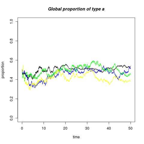
Figure 1: Global proportions of type $a$ individuals; one realisation, four different scenarios: blue anticorrelated environments, green correlated environments, black constant selection, and yellow neutral. See the main text for a full explanation.

In Figure 2, we have used a greyscale to record the proportion of type $a$ individuals in each deme - the darker the colour, the greater the proportion of type $a$. In the top left, selection is fixed, and we clearly see the effect of type $a$ being favoured in demes $50-100$. In the next two frames (top right and bottom left), the environment fluctuates, but whereas on the top left demes $0-50$ always favour the opposite type to demes $51-100$, on the bottom left all demes always favour the same type. The neutral model is the bottom right. When we repeat over many realisations, we see a greater concentration of types than for the neutral model, but it is certainly not easy to distinguish between the two frames.

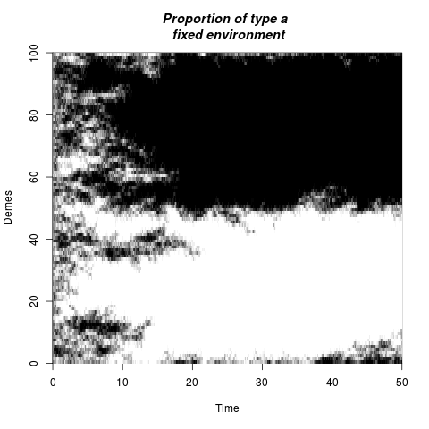
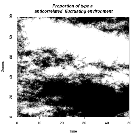
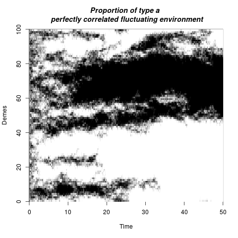
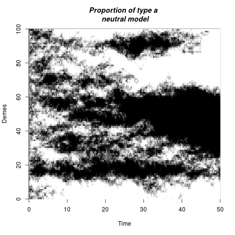
Figure 2: Map of the proportion of type $a$ individuals in each deme; the darker the colour the higher the proportion of type $a$. Top left, constant selection; top right, fluctuating selection with demes $0-50$ and $51-100$ perfectly anticorrelated; bottom left, fluctuating selection with all demes perfectly correlated; bottom right, the neutral case.

Just following the overall proportion of types in a deme is throwing away a lot of information, which may be available in genetic data, about the distribution of families. To explore this we used ‘tracers’, further explored in the context of Spatial Lambda-Fleming-Viot process in Section 6. In Figure 3 we mark individuals descended from the population in particular demes at time zero. The darker the colour, the higher the proportion of marked individuals. In a constant environment, left panel, the surviving family is well adapted to the environment in demes $50-100$, but has difficulty invading demes $1-50$, where it is not favoured. It also struggles to expand beyond deme $80$. This turns out to be because of competition with the equally well adapted family that is descended from individuals that were in deme $84$ at time zero (right hand panel).

Figure 3: Tracer map of individuals descended from ancestors located in particular demes at time zero; the darker the colour, the higher the proportion of such individuals. Fixed environment.

In left panel of Figure 4, we see a successful family in a fluctuating environment (with demes $0-50$ and $51-100$ perfectly anticorrelated). The family is on the brink of extinction several times and is rescued by a change in the environment. In the right panel, we see a family that begins life right on the boundary between the two regions. The environments are perfectly anticorrelated and the family is able to survive and spread much more readily.

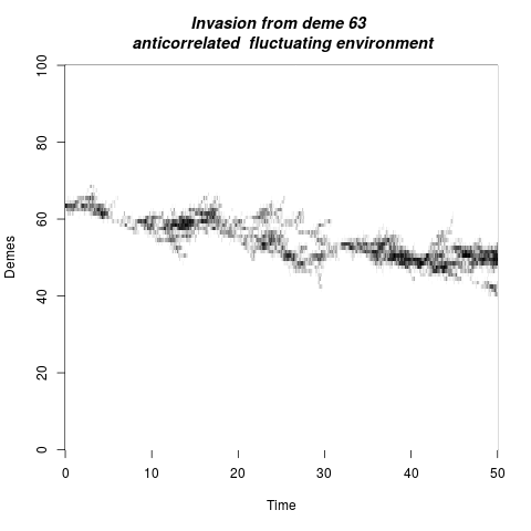
Figure 4: Tracer map of individuals descended from ancestors located in particular demes at time zero; the darker the colour, the higher the proportion of such individuals. The environment is fluctuating, with its value in demes $0-50$ perfectly anticorrelated with that in demes $51-100$.

The right hand panel of Figure 4 can be contrasted with the left hand panel of Figure 5. The descendants of ancestors in deme $1$ find it harder to spread in a perfectly correlated environment than in the perfectly anticorrelated environment of the previous figure. The trace of descendants of ancestors in deme $78$ in the right hand panel of Figure 5 shows the ‘thinning’ of the family resulting from the periods of time when it is not favoured.

Figure 5: Tracer map of individuals descended from ancestors located in particular demes at time zero; the darker the colour, the higher the proportion of such individuals. The environment is fluctuating, with its value in demes $0-50$ perfectly correlated with that in demes $51-100$.

Finally, Figure 6, shows the trace of descendants of ancestors in demes $12$ and $16$ for the neutral model. There appears to be a barrier between the two families, which could easily be mistaken for a change in the environment somewhere between demes $12$ and $16$, on the lower side of which the family descended from deme $12$ is better adapted and on the upper side of which the family from deme $16$ is better adapted. In fact this is due to competition between two equally fit families.

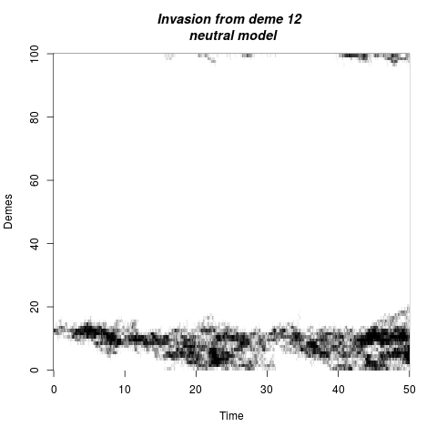
Figure 6: Tracer map of individuals descended from ancestors located in particular demes at time zero; the darker the colour, the higher the proportion of such individuals. Neutral model.

8 Proof of Theorem 4.6

The proof of Theorem 4.6 will rest on Theorem 2.1 of Kurtz (1992) (or rather his Example 2.2). For a metric space $E$, let $l_{m}(E)$ be the space of measures on $[0,\infty)\times E$ such that $\mu\in l_{m}(E)$ if $\mu([0,t)\times E)=t$.

Theorem 8.1 ( Kurtz (1992), Theorem 2.1).

Let $E_{1}$, $E_{2}$ be complete separable metric spaces, and set $E=E_{1}\times E_{2}$. For each $n$, let $\{(X_{n},Y_{n})\}$ be a stochastic process with sample paths in $D_{E}([0,\infty))$ adapted to a filtration $\{{\cal F}_{t}^{n}\}$. Assume that $\{X_{n}\}$ satisfies the compact containment condition, that is, for each $\epsilon>0$ and $T>0$, there exists a compact $K\subset E_{1}$ such that

$$\inf_{n}\mathbb{P}[X_{n}(t)\in K,t\leq T]\geq 1-\epsilon,$$ (8.1)

and assume that $\{Y_{n}(t):t\geq 0,n=1,2,\ldots\}$ is relatively compact (as a collection of $E_{2}$-valued random variables). Suppose that there is an operator $A:{\cal D}(A)\subset\overline{C}(E_{1})\rightarrow C(E_{1}\times E_{2})$ such that for $f\in{\cal D}(A)$ there is a process $\epsilon_{n}^{f}$ for which

$$f(X_{n}(t))-\int_{0}^{t}Af(X_{n}(s),Y_{n}(s))\mathrm{d}s+\epsilon_{n}^{f}(t)$$ (8.2)

is an $\{{\cal F}_{t}^{n}\}$-martingale. Let ${\cal D}(A)$ be dense in $\overline{C}(E_{1})$ in the topology of uniform convergence on compact sets. Suppose that for each $f\in{\cal D}(A)$ and each $T>0$, there exists $p>1$ such that

$$\sup_{n}\mathbb{E}\left[\int_{0}^{T}|Af(X_{n}(t),Y_{n}(t)|^{p}\mathrm{d}t\right]<\infty$$ (8.3)

and

$$\lim_{n\rightarrow\infty}\mathbb{E}\left[\sup_{t\leq T}|\epsilon_{n}^{f}(t)|\right]=0.$$ (8.4)

Let $\Gamma_{n}$ be the $l_{m}(E_{2})$-valued random variable given by

$$\Gamma_{n}\left([0,t]\times B\right)=\int_{0}^{t}\mathbf{1}_{B}(Y_{n}(s))\mathrm{d}s.$$

Then $\{(X_{n},\Gamma_{n})\}$ is relatively compact in $D_{E_{1}}[0,\infty)\times l_{m}(E_{2})$, and for any limit point $(X,\Gamma)$ there exists a filtration $\{{\cal G}_{t}\}$ such that

$$f(X(t))-\int_{0}^{t}\int_{E_{2}}Af(X(s),y)\Gamma(\mathrm{d}s\times\mathrm{d}y)$$ (8.5)

is a $\{{\cal G}_{t}\}$-martingale for each $f\in{\cal D}(A)$.

As a particular case, Kurtz (1992) provides the following example.

Example 8.2 ( Kurtz (1992), Example 2.2).

Suppose $Y$ is stationary and ergodic, and $Y_{n}$ in Theorem 8.1 is given by $Y_{n}(t)\equiv Y(nt)$. Then $\Gamma=m\times\pi$ where $m$ denotes Lebesgue measure and $\pi$ is the marginal distribution for $Y$. Consequently, under the assumptions of Theorem 8.1, $X$ is a solution of the martingale problem for $C$ given by

$$Cf(x)=\int Af(x,y)\pi(\mathrm{d}y),\qquad f\in{\cal D}(A).$$

Let us briefly discuss how our setup fits into that of Theorem 8.1. The sequence of measure-valued evolutions $\big{(}\overline{M}^{n}_{t}\big{)}_{t\geq 0}$ corresponds to the process $X_{n}$, while the sequence of environments corresponds to the process $Y_{n}$. Notice that $Y_{n}$ defined that way satisfies the assumptions of Example 8.2, and therefore those of Theorem 8.1. The domain of the generator $A$ is given by the closure of

$$\mathcal{D}(A)=\bigg{\{}F(\langle\cdot,w\rangle):f\in C_{c}^{\infty}(\mathbb{R}^{d}),F\in C^{\infty}(\mathbb{R})\bigg{\}}.$$ (8.6)

Since the state space of $\big{(}\overline{M}^{n}_{t}\big{)}_{t\geq 0}$ is compact, the compact containment condition (8.1) is satisfied.

The key step in applying Theorem 8.1 is the identification of the generator $A$, which leads to the decomposition (8.2). This consists of two steps. First we approximate the part of the SLFVFS generator corresponding to neutral events, and second we deal with the terms corresponding to fluctuating selection. These two steps are accomplished in Subsection 8.1.

Our approach mirrors the strategy of Section 3. Having transformed the generator of the SLFVFS into a form which allows us to consider the process of averaged densities $\overline{w}^{n}_{t}$, we use the ‘separation of timescales’ trick of Kurtz (1973), to (up to a small error) split the generator into parts corresponding to neutral and selective events in a convenient way; see equation (8.1). We then consider the two terms in this decomposition. The analysis of the neutral part of the generator will closely follow Etheridge et al. (2018); the novel step is the second, which deals with the terms corresponding to fluctuating selection. Our analysis will not only identify the correct form of $A$ and $\epsilon_{n}^{f}$ (see (8.28) and (8.29) respectively), but also provides a uniform bound on $A$, which shows that (8.3) is satisfied.

Having identified $A$, and $\epsilon_{n}^{f}$, we show that (8.4) holds. This bound relies on the Lipschitz bound (4.3) on the correlation kernel $g(x,y)$. Subsection 8.1 concludes with a discussion of the continuity estimates on the averaged densities of the measure-valued evolutions that are required to deduce our result. These estimates are stated as Equation (8.30) and Proposition 8.5 (and proved in Appendix A). This leads to a complete characterisation of limits of the sequence of averaged processes $\overline{w}_{n}$ as solutions to a martingale problem.

In Subsection 8.2 we discuss the uniqueness of solution to the limiting martingale problem, which we have only managed to prove in dimensions $d\geq 2$. This requires a separate argument based on the fact that, under certain regularity conditions (which are satisfied as a result of Proposition 8.5), any solution to the martingale problem is a weak solution to a corresponding stochastic p.d.e. The weak uniqueness of solutions to the stochastic p.d.e. is a consequence of a combination of a pathwise uniqueness result of Rippl and Sturm (2013) and a Yamada-Watanabe Theorem.

8.1 Identifying the limit

In what follows $C$ is a constant that depends on certain fixed quantities such as the functions $f$ and $F$ that appear in our test functions, c.f. (8.6), and the quantities $\mathbf{s}$ and $\bar{u}$ appearing in our scaled selection and impact parameters in the statement of Theorem 4.6. The quantity $C$ may vary from line to line; its exact value is unimportant.

Throughout this section we shall be manipulating expressions pertaining to a local average of a version of the density of the SLFVFS. These manipulations are insensitive to changing that density on a set of Lebesgue measure zero and so should really be thought of as results for the measure-valued evolution itself.

Our result concerns the locally averaged process $\overline{w}_{n}$. However, before passage to the limit, this process is not Markov (in contrast to $w$ itself). In order to overcome this, we follow Etheridge et al. (2018) and define

$$\phi_{f}(x)=\mathchoice{\mathop{\kern 1.99997pt\vrule width=6.00006pt,height=3.0pt,depth=-2.49997pt\kern-8.00003pt\intop}\nolimits_{\kern-2.79996ptB_{n}(x)}}{\mathop{\kern 1.00006pt\vrule width=5.0pt,height=3.0pt,depth=-2.59996pt\kern-6.00006pt\intop}\nolimits_{B_{n}(x)}}{\mathop{\kern 1.00006pt\vrule width=5.0pt,height=3.0pt,depth=-2.59996pt\kern-6.00006pt\intop}\nolimits_{B_{n}(x)}}{\mathop{\kern 1.00006pt\vrule width=5.0pt,height=3.0pt,depth=-2.59996pt\kern-6.00006pt\intop}\nolimits_{B_{n}(x)}}f(y)\mathrm{d}y.$$

To alleviate notation, we have suppressed the dependence on $n$ in this quantity. Notice that

$$\langle w_{n},\phi_{f}\rangle=\int_{\mathbb{R}^{d}}\int_{\mathbb{R}^{d}}w_{n}(y)\frac{n^{\frac{d}{3}}}{V_{R}}f(z)\mathbf{1}_{\{|z-y|\leq R_{n}\}}(z)\mathrm{d}y\mathrm{d}z=\langle\overline{w}_{n},f\rangle.$$

Using Taylor’s Theorem, we see that for $f\in C^{2}_{c}$,

$$\phi_{f}(x) =f(x)+\frac{n^{\frac{d}{3}}}{V_{R}}\int_{B_{n}(x)}(y-x)\cdot\nabla f(x)\mathrm{d}y+\mathcal{O}\left(\frac{n^{\frac{d}{3}}}{V_{R}}\int_{B_{n}(x)\cap S_{f}}|x-y|^{2}\mathrm{d}x\right)$$

$$=f(x)+\mathcal{O}\left(n^{-\frac{2}{3}}\right)\mathbf{1}_{B_{n}(x)\cap S_{f}\neq\emptyset},$$ (8.7)

where $S_{f}$ denotes the support of $f$. Here, and throughout, we have used $|\cdot|$ to denote the Euclidean norm. This yields the useful approximation

$$\langle\overline{w}_{n},f\rangle=\langle w_{n},\phi_{f}\rangle=\langle w_{n},f\rangle+\mathcal{O}(n^{-\frac{2}{3}}).$$ (8.8)

It will be convenient to have some notation.

Notation 8.3.

Suppose that immediately before a reproduction event the unscaled process takes the value $w$, then immediately after the event, its state will be $\theta^{+}_{x,R,\bar{u}}(w)$, if the parent of the event was of type $a$, and $\theta^{-}_{x,R,\bar{u}}(w)$ if the parent was of type $A$, where

$$\theta^{+}_{x,R,\bar{u}}(w) =\mathbf{1}_{\mathbb{R}^{d}\setminus B(x,R)}w+\mathbf{1}_{B(x,R)}\left((1-\bar{u})w+\bar{u}\right),$$

$$\theta^{-}_{x,R,\bar{u}}(w) =\mathbf{1}_{\mathbb{R}^{d}\setminus B(x,R)}w+\mathbf{1}_{B(x,R)}(1-\bar{u})w.$$ (8.9)

Using this notation,

$$\big{\langle}\theta^{+}_{x,R_{n},u_{n}}(w),\phi_{f}\big{\rangle}-\langle w,\phi_{f}\rangle=u_{n}\left\langle\mathbf{1}_{B_{n}(x)}(1-w),\phi_{f}\right\rangle,$$ (8.10)

$$\big{\langle}\theta^{-}_{x,R_{n},u_{n}}(w),\phi_{f}\big{\rangle}-\left\langle w,\phi_{f}\right\rangle=-u_{n}\left\langle\mathbf{1}_{B_{n}(x)}w,\phi_{f}\right\rangle.$$ (8.11)

The first step will be to evaluate the generator on test functions of the form

$$\psi_{F,f}(w_{n})=F\left(\langle\overline{w}_{n},f\rangle\right)=F\left(\langle w_{n},\phi_{f}\rangle\right),$$ (8.12)

where $F\in C^{\infty}(\mathbb{R})$, $f\in C^{\infty}_{c}(\mathbb{R}^{d})$. Notice that these are independent of the environment $\zeta$. Recall that the analogous functions were our starting point in Section 3. Since the support $S_{f}$ of $f$ is compact, it is only overlapped by events at a finite rate and so, writing ${\cal L}\psi_{F,f}$, which will be a function of the state $\zeta(\cdot)$ of the environment, for the generator of the unscaled process acting on test functions of this form, we have

$$\mathcal{L}\psi_{F,f}(w,\zeta) = (1-{\mathbf{s}})\int_{\mathbb{R}^{d}}\mathchoice{\mathop{\kern 1.99997pt\vrule width=6.00006pt,height=3.0pt,depth=-2.49997pt\kern-8.00003pt\intop}\nolimits_{\kern-2.79996ptB(x,R)}}{\mathop{\kern 1.00006pt\vrule width=5.0pt,height=3.0pt,depth=-2.59996pt\kern-6.00006pt\intop}\nolimits_{B(x,R)}}{\mathop{\kern 1.00006pt\vrule width=5.0pt,height=3.0pt,depth=-2.59996pt\kern-6.00006pt\intop}\nolimits_{B(x,R)}}{\mathop{\kern 1.00006pt\vrule width=5.0pt,height=3.0pt,depth=-2.59996pt\kern-6.00006pt\intop}\nolimits_{B(x,R)}}w(y)\left[F(\langle\theta^{+}_{x,R,\bar{u}}(w),\phi_{f}\rangle)-F(\langle w,\phi_{f}\rangle)\right]\mathrm{d}y\mathrm{d}x$$

$$+(1-\mathbf{s})\int_{\mathbb{R}^{d}}\mathchoice{\mathop{\kern 1.99997pt\vrule width=6.00006pt,height=3.0pt,depth=-2.49997pt\kern-8.00003pt\intop}\nolimits_{\kern-2.79996ptB(x,R)}}{\mathop{\kern 1.00006pt\vrule width=5.0pt,height=3.0pt,depth=-2.59996pt\kern-6.00006pt\intop}\nolimits_{B(x,R)}}{\mathop{\kern 1.00006pt\vrule width=5.0pt,height=3.0pt,depth=-2.59996pt\kern-6.00006pt\intop}\nolimits_{B(x,R)}}{\mathop{\kern 1.00006pt\vrule width=5.0pt,height=3.0pt,depth=-2.59996pt\kern-6.00006pt\intop}\nolimits_{B(x,R)}}\{1-w(y)\}\left[F(\langle\theta^{-}_{x,R,\bar{u}}(w),\phi_{f}\rangle)-F(\langle w,\phi_{f}\rangle)\right]\mathrm{d}y\mathrm{d}x$$

$$+\mathbf{s}\int_{\mathbb{R}^{d}}\mathchoice{\mathop{\kern 1.99997pt\vrule width=6.00006pt,height=3.0pt,depth=-2.49997pt\kern-8.00003pt\intop}\nolimits_{\kern-2.79996ptB(x,R)^{2}}}{\mathop{\kern 1.00006pt\vrule width=5.0pt,height=3.0pt,depth=-2.59996pt\kern-6.00006pt\intop}\nolimits_{B(x,R)^{2}}}{\mathop{\kern 1.00006pt\vrule width=5.0pt,height=3.0pt,depth=-2.59996pt\kern-6.00006pt\intop}\nolimits_{B(x,R)^{2}}}{\mathop{\kern 1.00006pt\vrule width=5.0pt,height=3.0pt,depth=-2.59996pt\kern-6.00006pt\intop}\nolimits_{B(x,R)^{2}}}\Bigg{\{}w(y_{1})w(y_{2})+\frac{1-\zeta(x)}{2}\Bigg{[}(w(y_{1})(1-w(y_{2}))$$

$$+(1-w(y_{2}))w(y_{2})\Bigg{]}\Bigg{\}}\times\left[F(\langle\theta^{+}_{x,R,\bar{u}}(w),\phi_{f}\rangle)-F(\langle w,\phi_{f}\rangle)\right]\mathrm{d}y_{1}\mathrm{d}y_{2}\mathrm{d}x$$

$$+\mathbf{s}\int_{\mathbb{R}^{d}}\mathchoice{\mathop{\kern 1.99997pt\vrule width=6.00006pt,height=3.0pt,depth=-2.49997pt\kern-8.00003pt\intop}\nolimits_{\kern-2.79996ptB(x,R)^{2}}}{\mathop{\kern 1.00006pt\vrule width=5.0pt,height=3.0pt,depth=-2.59996pt\kern-6.00006pt\intop}\nolimits_{B(x,R)^{2}}}{\mathop{\kern 1.00006pt\vrule width=5.0pt,height=3.0pt,depth=-2.59996pt\kern-6.00006pt\intop}\nolimits_{B(x,R)^{2}}}{\mathop{\kern 1.00006pt\vrule width=5.0pt,height=3.0pt,depth=-2.59996pt\kern-6.00006pt\intop}\nolimits_{B(x,R)^{2}}}\Bigg{\{}(1-w(y_{1}))(1-w(y_{2}))+\frac{1+\zeta(x)}{2}(w(y_{1})(1-w(y_{2}))$$

$$+(1-w(y_{1}))w(y_{2}))\Bigg{\}}\times\left[F(\langle\theta^{-}_{x,R,\bar{u}}(w),\phi_{f}\rangle)-F(\langle w,\phi_{f}\rangle)\right]\mathrm{d}y_{1}\mathrm{d}y_{2}\mathrm{d}x.$$

$$:= \mathcal{L}^{neu}\psi_{F,f}(w)+\mathcal{L}^{fsel}\psi_{F,f}(w,\zeta)$$

We recognise the generator of the neutral spatial Lambda-Fleming-Viot process (which does not depend on the environment) plus two terms reflecting the selection events. If we set the environment to be identically equal to $1$, say, then the surviving selection term is precisely that considered in Etheridge et al. (2018) in modelling selection in favour of type $A$ individuals.

After scaling (and a change of variables), the generator of $w_{n}$ acting on test functions of this form is given by

$$\mathcal{L}_{n}\psi_{F,f}(w_{n},\zeta) =n^{1+\frac{d}{3}}(1-\mathbf{s}_{n})\left(\int_{\mathbb{R}^{d}}\overline{w}_{n}(x)\left[F(\langle\theta^{+}_{x,R_{n},u_{n}}(w_{n}),\phi_{f}\rangle)-F(\langle w_{n},\phi_{f}\rangle)\right]\mathrm{d}x\right.$$

$$\phantom{=n^{1+\frac{d}{3}}}+\left.\int_{\mathbb{R}^{d}}\{1-\overline{w}_{n}(x)\}\left[F(\langle\theta^{-}_{x,R_{n},u_{n}}(w_{n}),\phi_{f}\rangle)-F(\langle w_{n},\phi_{f}\rangle)\right]\mathrm{d}x\right)$$

$$+n^{1+\frac{d}{3}}\mathbf{s}_{n}\int_{\mathbb{R}^{d}}\left\{\overline{w}_{n}^{2}(x)+(1-\zeta(x))\overline{w}_{n}(x)(1-\overline{w}_{n}(x))\right\}$$

$$\phantom{=n^{1+\frac{d}{3}}=n^{1+\frac{d}{3}}=n^{1+\frac{d}{3}}\mathbf{s}_{n}\int_{\mathbb{R}^{d}}}\times\left[F(\langle\theta^{+}_{x,R_{n},u_{n}}(w_{n}),\phi\rangle)-F(\langle w_{n},\phi_{f}\rangle)\right]\mathrm{d}x$$

$$+n^{1+\frac{d}{3}}\mathbf{s}_{n}\int_{\mathbb{R}^{d}}\left\{(1-\overline{w}_{n}(x))^{2}+(1+\zeta(x))\overline{w}_{n}(x)(1-\overline{w}(x))\right\}$$

$$\phantom{=n^{1+\frac{d}{3}}=n^{1+\frac{d}{3}}=n^{1+\frac{d}{3}}\mathbf{s}_{n}\int_{\mathbb{R}^{d}}}\times\left[F(\langle\theta^{-}_{x,R_{n},u_{n}}(w_{n}),\phi_{f}\rangle)-F(\langle w_{n},\phi_{f}\rangle)\right]\mathrm{d}x.$$

By analogy with (3.3), we write this as

$$\mathcal{L}_{n}\psi_{F,f}=(1-{\mathbf{s}}_{n})\mathcal{L}^{neu}_{n}\psi_{F,f}+n^{\alpha}\mathcal{L}^{fsel}_{n}\psi_{F,f},$$ (8.13)

where

$$\mathcal{L}^{neu}_{n}\psi_{F,f}(w_{n})=n^{1+\frac{d}{3}}\left(\int_{\mathbb{R}^{d}}\overline{w}_{n}(x)\left[F(\langle\theta^{+}_{x,R_{n},u_{n}}(w_{n}),\phi_{f}\rangle)-F(\langle w_{n},\phi_{f}\rangle)\right]\mathrm{d}x\right.\\ \left.+\int_{\mathbb{R}^{d}}\{1-\overline{w}_{n}(x)\}\left[F(\langle\theta^{-}_{x,R_{n},u_{n}}(w_{n}),\phi_{f}\rangle)-F(\langle w_{n},\phi_{f}\rangle)\right]\mathrm{d}x\right),$$ (8.14)

and, writing ${\mathbf{s}}_{n}=n^{\alpha}\tilde{\mathbf{s}}_{n}=n^{\alpha}{\mathbf{s}}/n^{2/3}$,

$$\mathcal{L}^{fsel}_{n}\psi_{F,f}(w_{n},\zeta) =n^{1+\frac{d}{3}}\tilde{\mathbf{s}}_{n}\int_{\mathbb{R}^{d}}\left\{\overline{w}_{n}(x)-\zeta(x)\overline{w}_{n}(x)(1-\overline{w}_{n}(x))\right\}$$

$$\phantom{\mathcal{L}^{fsel}_{n}F(\langle w_{n},\phi_{f}\rangle)}\times\left[F(\langle\theta^{+}_{x,R_{n},u_{n}}(w_{n}),\phi_{f}\rangle)-F(\langle w_{n},\phi_{f}\rangle)\right]\mathrm{d}x$$

$$+n^{1+\frac{d}{3}}\tilde{\mathbf{s}}_{n}\int_{\mathbb{R}^{d}}\left\{(1-\overline{w}_{n}(x))+\zeta(x)\overline{w}_{n}(x)(1-\overline{w}_{n}(x))\right\}$$

$$\phantom{\mathcal{L}^{fsel}_{n}F(\langle w_{n},\phi_{f}\rangle)}\times\left[F(\langle\theta^{-}_{x,R_{n},u_{n}}(w_{n}),\phi_{f}\rangle)-F(\langle w_{n},\phi_{f}\rangle)\right]\mathrm{d}x.$$

Just as in the non-spatial case, in order to reduce the generator to the form (8.2), we appeal to the approach of Kurtz (1973). Entirely analogously to our calculations of Section 3 (see (3.4)), we evaluate the generator on test functions of the form

$$G_{F,f}(w_{n},\zeta)=\psi_{F,f}(w_{n})+n^{-\alpha}\mathcal{L}^{fsel}_{n}\psi_{F,f}(w_{n},\zeta),$$ (8.15)

where $F\in C^{\infty}(\mathbb{R})$ and $f\in C_{c}^{\infty}(\mathbb{R}^{d})$. The second term on the right hand side will form part of $\epsilon_{n}^{f}$ in (8.2). Evidently we must now account for the changing environment, but this is just the generator of a pure jump process in which a new state is sampled from a (mean zero) stationary distribution at the times of a Poisson process of rate $n^{2\alpha}\tau^{env}$.

Writing the full generator as ${\cal L}^{neu}+n^{\alpha}{\cal L}^{fsel}+n^{2\alpha}{\cal L}^{env}$, as in (3.3), we observe that ${\cal L}^{env}\psi_{F,f}=0$ (since $\psi_{F,f}$ is independent of $\zeta$). In (8.23) below, we show that

$${\cal L}^{fsel}\psi_{F,f}(w_{n},\zeta)=-{\mathbf{s}}\bar{u}V_{R}F^{\prime}(\langle w_{n},\phi_{f}\rangle)\int\zeta(x)\overline{w}_{n}(x)\left(1-\overline{w}_{n}(x)\right)f(x)\mathrm{d}x+\mathcal{O}\left(n^{-\frac{1}{3}}\right),$$

and since $\mathbb{E}_{\pi}[\zeta]=0$, $\mathbb{E}_{\pi}[{\cal L}^{fsel}\psi_{F,f}]=\mathcal{O}(n^{-1/3})$. Calculating exactly as in the non-spatial case (see (3.5)), we find a spatial analogue of (3.6), that is

$$\mathcal{L}_{n}G_{F,f}(w_{n},\zeta)+\mathcal{O}\left(n^{-\alpha}\right) =\mathcal{L}^{neu}_{n}\psi_{F,f}(w_{n})+\mathcal{L}^{fsel}_{n}\left(\mathcal{L}^{fsel}_{n}\psi_{F,f}\right)(w_{n},\zeta)$$

$$:=\mathcal{L}^{neu}_{n}\psi_{F,f}(w_{n})+\mathcal{G}_{n}\psi_{F,f}(w_{n},\zeta),$$ (8.16)

where we have used that $\alpha<1/6<1/3$ to absorb $\mathbb{E}_{\pi}[{\cal L}^{fsel}\psi_{F,f}]$ into the error on the left hand side. In this notation, for $F\in C^{\infty}(\mathbb{R})$ and $f\in C^{\infty}_{c}(\mathbb{R}^{d})$

$$\psi_{F,f}(w_{n}(t))-\int_{0}^{t}\left[\mathcal{L}_{n}^{neu}\psi_{F,f}\left(w_{n}(s)\right)+\mathcal{G}_{n}\psi_{F,f}\left(w_{n}(s),\zeta(s)\right)\right]\mathrm{d}s+\mathcal{O}\left(n^{-\alpha}\right)$$

is a martingale.

Neutral part

First we find an approximation to the part of the generator corresponding to neutral events. This mirrors the proof of Theorem 1.8 of Etheridge et al. (2018) and so we recall the strategy, but omit many of the details.

Taking the expression (8.14) for ${\cal L}_{n}^{neu}$, we perform a Taylor expansion of $F$ about $\langle w_{n},\phi_{f}\rangle$ to obtain

$$\int_{0}^{t}\mathcal{L}_{n}^{neu}\psi_{F,f}\left(w_{n}(s)\right)\mathrm{d}s=(1-\mathbf{s}_{n})\int_{0}^{t}\left[A_{n}(s)+B_{n}(s)+C_{n}(s)\right]\mathrm{d}s,$$

where $A_{n}(s)$, $B_{n}(s)$, $C_{n}(s)$ can be expressed as

$$A_{n}(s) =u_{n}n^{1+\frac{d}{3}}F^{\prime}\left(\langle\overline{w}_{n}(s),f\rangle\right)\int_{\mathbb{R}^{d}}\left[\overline{w}_{n}(s,x)\left\langle\mathbf{1}_{B_{n}(x)}\left(1-w_{n}(s)\right),\phi_{f}\right\rangle\right.$$

$$\phantom{{}=u_{n}n^{1+\frac{d}{3}}F^{\prime}\left(\langle\overline{w}_{n}(t),f\rangle\right)\int_{\mathbb{R}^{d}}}\left.-\left(1-\overline{w}_{n}(s,x)\right)\left\langle\mathbf{1}_{B_{n}(x)}w_{n}(s),\phi_{f}\right\rangle\right]\mathrm{d}x$$

$$B_{n}(s) =u_{n}^{2}n^{1+\frac{d}{3}}\frac{F^{\prime\prime}\left(\langle\overline{w}_{n}(s),f\rangle\right)}{2}\int_{\mathbb{R}^{d}}\left[\overline{w}_{n}(s,x)\left\langle\mathbf{1}_{B_{n}(x)}\left(1-w_{n}(s)\right),\phi_{f}\right\rangle^{2}\right.$$

$$\phantom{{}=u_{n}n^{1+\frac{d}{3}}F^{\prime}\left(\langle\overline{w}^{n}(t),f\rangle\right)\int_{\mathbb{R}^{d}}}\left.+\left(1-\overline{w}_{n}(s,x)\right)\left\langle\mathbf{1}_{B_{n}(x)}w_{n}(s),\phi_{f}\right\rangle^{2}\right]\mathrm{d}x$$

$$C_{n}(s) \leq\mathcal{O}(n^{-2d/3}),$$

where we have used (8.10) and (8.11) and $C_{n}$ corresponds to the third order term in the Taylor expansion.

The key to controlling $A_{n}$ and $B_{n}$ is a Taylor expansion of $\phi_{f}$. First we use Fubini’s Theorem to write

$$A_{n}(s) =u_{n}n^{1+\frac{d}{3}}F^{\prime}\left(\langle\overline{w}_{n}(s),f\rangle\right)\int_{\mathbb{R}^{d}}\left\{\overline{w}_{n}(s,x)\langle\mathbf{1}_{B_{n}(x)},\phi_{f}\rangle-\langle\mathbf{1}_{B_{n}(x)}w_{n}(s),\phi_{f}\rangle\right\}\mathrm{d}x$$

$$=u_{n}n^{1+\frac{d}{3}}F^{\prime}\left(\langle\overline{w}_{n}(s),f\rangle\right)\int_{\mathbb{R}^{d}}\left[\frac{n^{\frac{d}{3}}}{V_{R}}\int_{\mathbb{R}^{d}}\int_{\mathbb{R}^{d}}\mathbf{1}_{\{|x-y|<R_{n}\}}w_{n}(s,y)\mathbf{1}_{\{|x-z|<R_{n}\}}\phi_{f}(z)\mathrm{d}y\mathrm{d}z\right.$$

$$\phantom{=u_{n}n^{1+\frac{d}{3}}u_{n}n^{1+\frac{d}{3}}u_{n}n^{1+\frac{d}{3}}F^{\prime}\left(\langle\overline{w}_{n}(s),f\rangle\right)\int_{\mathbb{R}^{d}}}\left.-\int_{\mathbb{R}^{d}}\mathbf{1}_{\{|x-y|<R_{n}\}}w_{n}(s,y)\phi_{f}(y)\mathrm{d}y\right]\mathrm{d}x$$

$$=u_{n}n^{1+\frac{d}{3}}F^{\prime}\left(\langle\overline{w}_{n}(s),f\rangle\right)\int_{\mathbb{R}^{d}}\frac{n^{\frac{d}{3}}}{V_{R}}\int_{\mathbb{R}^{d}}\int_{\mathbb{R}^{d}}\mathbf{1}_{\{|x-y|<R_{n}\}}w_{n}(s,y)\mathbf{1}_{\{|x-z|<R_{n}\}}$$

$$\phantom{u_{n}n^{1+\frac{d}{3}}F^{\prime}\left(\langle\overline{w}_{n}(s),f\rangle\right)\int_{\mathbb{R}^{d}}\frac{n^{\frac{d}{3}}}{V_{R}}\int_{\mathbb{R}^{d}}\int_{\mathbb{R}^{d}}\mathbf{1}_{\{|x-y|<R_{n}\}}w_{n}(s,y)}\left(\phi_{f}(z)-\phi_{f}(y)\right)\mathrm{d}y\mathrm{d}z\mathrm{d}x.$$

Now Taylor-expand $\phi_{f}$ around $y$ to obtain

$$A_{n}(s)=u_{n}n^{1+\frac{d}{3}}F^{\prime}\left(\langle\overline{w}_{n}(s),f\rangle\right)\int_{\mathbb{R}^{d}}\left[\frac{n^{\frac{d}{3}}}{V_{R}}\int\int\mathbf{1}_{\{|x-y|<R_{n}\}}w_{n}(s,y)\mathbf{1}_{\{|x-z|<R_{n}\}}\right.\\ \left.\times\left[D\phi_{f}(y)(z-y)+\frac{1}{2}(z-y){\mathbf{H}}(y)\phi_{f}(z-y)+\mathcal{O}\left(|z-y|^{3}\right)\mathbf{1}_{y\in S_{f}}\right]\right]\mathrm{d}y\mathrm{d}z\mathrm{d}x,$$ (8.17)

where ${\mathbf{H}}$ denotes the Hessian. Using anti-symmetry of $z-y$, the term involving the gradient vanishes, as do the off-diagonal terms in the Hessian, so that (8.17) is equal to

$$u_{n}n^{1+\frac{d}{3}}F^{\prime}\left(\langle\overline{w}_{n}(s),f\rangle\right)\int_{\mathbb{R}^{d}}\frac{n^{\frac{d}{3}}}{V_{R}}\int_{\mathbb{R}^{d}}\int_{\mathbb{R}^{d}}\mathbf{1}_{\{|x-y|<R_{n}\}}\mathbf{1}_{\{|x-z|<R_{n}\}}w_{n}(s,y)$$

$$\times\frac{1}{2}\sum_{i=1}^{d}(z_{i}-y_{i})^{2}\frac{\partial^{2}}{\partial y_{i}^{2}}\phi_{f}(y)\mathrm{d}y\mathrm{d}z\mathrm{d}x,$$

plus a lower order term which is bounded uniformly in the time variable $s$ by $\mathtt{Vol}(S_{f})u_{n}C_{f}$ (where $C_{f}$ is a bound on the third derivative of $f$ and $S_{f}$ is the support of $f$). The analogue of (8.1) with $\phi_{f}$ replaced by $\frac{\partial^{2}\phi_{f}}{\partial y_{i}^{2}}$ is

$$\frac{\partial^{2}}{\partial y_{i}^{2}}\phi_{f}(y)=\frac{\partial^{2}f}{\partial y_{i}^{2}}(y)+\mathcal{O}(n^{-2/3}\mathbf{1}_{B_{n}(y)\cap S_{f}\neq\emptyset}),$$

and (using (8.8) with $\Delta f$ in place of $f$) we deduce that

$$A_{n}(s) =u_{n}n^{1+\frac{d}{3}}F^{\prime}\left(\langle\overline{w}_{n}(s),f\rangle\right)\int_{\mathbb{R}^{d}}\frac{n^{\frac{d}{3}}}{V_{R}}\int_{\mathbb{R}^{d}}\int_{\mathbb{R}^{d}}\mathbf{1}_{\{|x-y|<R_{n}\}}\mathbf{1}_{\{|x-z|<R_{n}\}}w_{n}(s,y)$$

$$\phantom{A_{n}(s)=u_{n}n^{1+\frac{d}{3}}}\times\frac{1}{2}\sum_{i=1}^{d}(z_{i}-y_{i})^{2}\frac{\partial^{2}}{\partial y_{i}^{2}}{f}(y)\mathrm{d}y\mathrm{d}z\mathrm{d}x+\mathcal{O}\left(n^{-\frac{2}{3}}C\right)$$

$$=\frac{\bar{u}\Gamma_{R}}{2}F^{\prime}\left(\langle\overline{w}_{n}(s),f\rangle\right)\int_{\mathbb{R}^{d}}w_{n}(s,y)\Delta f\mathrm{d}y+\mathcal{O}\left(n^{-\frac{2}{3}}C\right)$$

$$=\frac{\bar{u}\Gamma_{R}}{2}F^{\prime}\left(\langle\overline{w}_{n}(s),f\rangle\right)\langle\overline{w}_{n}(s),\Delta f\rangle+\mathcal{O}\left(n^{-\frac{2}{3}}C\right)$$ (8.18)

where

$$\Gamma_{R}=\frac{1}{V_{R}}\int_{B(0,R)}\int_{B(x,R)}(z_{1})^{2}\mathrm{d}z\mathrm{d}x,$$ (8.19)

and $z_{1}$ is the first component of the vector $z\in\mathbb{R}^{d}$. The error term tends to zero uniformly in $s$ and since $|\langle\overline{w}_{n}(s),f\rangle|\leq\|f\|_{\infty}\mathtt{Vol}(S_{f})$, we have that $|A_{n}(s)|$ is uniformly bounded in $s$ and $n$. The contribution coming from $B_{n}(s)$ can be treated similarly:

$$B_{n}(s)=u_{n}^{2}n^{1+\frac{d}{3}}\frac{F^{\prime\prime}\left(\langle\overline{w}_{n}(s),f\rangle\right)}{2}\\ \times\int_{\mathbb{R}^{d}}\overline{w}_{n}(s,x)\left\langle\mathbf{1}_{B_{n}(x)}\big{(}1-w_{n}(s)\big{)},\phi_{f}\right\rangle^{2}+(1-\overline{w}_{n}(s,x))\left\langle\mathbf{1}_{B_{n}(x)}{w}_{n}(s),\phi_{f}\right\rangle^{2}\mathrm{d}x\\ =u_{n}^{2}n^{1+\frac{d}{3}}\frac{F^{\prime\prime}\left(\langle\overline{w}_{n}(s),f\rangle\right)}{2}\int_{\mathbb{R}^{d}}\big{\{}\overline{w}_{n}(s,x)\left\langle\mathbf{1}_{B_{n}(x)},\phi_{f}\right\rangle^{2}\\ -2\overline{w}_{n}(s,x)\left\langle\mathbf{1}_{B_{n}(x)},\phi_{f}\right\rangle\left\langle w_{n}(s)\mathbf{1}_{B_{n}(x)},\phi_{f}\right\rangle+\left\langle w_{n}(s)\mathbf{1}_{B_{n}(x)},\phi_{f}\right\rangle^{2}\bigg{\}}\mathrm{d}x\\ =u_{n}^{2}n^{1+\frac{d}{3}}\frac{F^{\prime\prime}\left(\langle\overline{w}_{n}(s),f\rangle\right)}{2}\int_{\mathbb{R}^{d}}\bigg{\{}\overline{w}_{n}(s,x)\left\langle\mathbf{1}_{B_{n}(x)},\phi_{f}\right\rangle\big{(}\left\langle\mathbf{1}_{B_{n}(x)},\phi_{f}\right\rangle-\left\langle\mathbf{1}_{B_{n}(x)}w_{n}(s),\phi_{f}\right\rangle\big{)}\\ -\left\langle\mathbf{1}_{B_{n}(x)}w_{n}(s),\phi_{f}\right\rangle\big{(}\overline{w}_{n}(s,x)\left\langle\mathbf{1}_{B_{n}(x)},\phi_{f}\right\rangle-\left\langle\mathbf{1}_{B_{n}(x)}w_{n}(s),\phi_{f}\right\rangle\big{)}\bigg{\}}\mathrm{d}x\\ \leq u_{n}^{2}n^{1+\frac{d}{3}}\frac{F^{\prime\prime}\left(\langle\overline{w}_{n}(s),f\rangle\right)}{2}\int_{S_{f}}2\mathtt{Vol}\left(B_{n}(x)\right)^{2}\|f\|_{\infty}^{2}\mathrm{d}x\leq Cn^{\frac{1-d}{3}},$$ (8.20)

which implies that the sequence of quadratic variations is not only tight, but also, for dimensions $d\geq 2$, it tends to $0$ uniformly on compact time sets. In other words, any randomness remaining in the limit in $d\geq 2$ will be due to the fluctuations in the environment.

In $d=1$, using (8.1) and a further Taylor expansion to approximate $\phi_{f}(y)$ by $f(x)$ for $y\in B_{n}(x)$ (up to an error of order $n^{-1/3}$) and that $n^{1/3}u_{n}=\overline{u}$, $n^{1/3}\mathtt{Vol}(B_{n})=V_{R}$, we have

$$B_{n}(s)=\overline{u}^{2}V_{R}^{2}\frac{F^{\prime\prime}\left(\langle\overline{w}_{n}(s),f\rangle\right)}{2}\int_{\mathbb{R}}\overline{w}_{n}(s,x)\left(1-\overline{w}_{n}(s,x)\right)f(x)^{2}\mathrm{d}x+\mathcal{O}\left(n^{-\frac{1}{3}}\right).$$ (8.21)

It is this term that (via an application of Proposition 8.5) leads to the final term in (4.4).

Fluctuating part

In order to tackle the part of the generator which describes the fluctuating selection, we need to understand the action of the operator $\mathcal{L}^{fsel}_{n}$ on $\mathcal{L}^{fsel}_{n}\psi_{F,f}(w_{n},\zeta)$. It is here that we must diverge from Etheridge et al. (2018).

As before, although the test function $\psi_{F,f}(w_{n})$ does not depend on the environment, the result of applying $\mathcal{L}^{fsel}_{n}$ to it is a function that does depend on the environment, to which we must then apply $\mathcal{L}^{fsel}_{n}$. Recall that $\tilde{\mathbf{s}}_{n}=\mathbf{s}/n^{2/3}$. We take a Taylor expansion of $F$ about $\langle w_{n},\phi_{f}\rangle$ to obtain

$$\mathcal{L}^{fsel}_{n}\psi_{F,f}(w_{n},\zeta)+\mathcal{O}\left(n^{-\frac{1}{3}}C_{f}\right)$$

$$=n^{1+\frac{d}{3}}\tilde{\mathbf{s}}_{n}u_{n}\left[\int_{\mathbb{R}^{d}}\left\{\overline{w}_{n}(x)-\zeta(x)\overline{w}_{n}(x)(1-\overline{w}_{n}(x))\right\}F^{\prime}(\langle w_{n},\phi_{f}\rangle)\langle\mathbf{1}_{B_{n}(x)}(1-w_{n}),\phi_{f}\rangle\mathrm{d}x\right.$$

$$-\left.\int_{\mathbb{R}^{d}}\left\{(1-\overline{w}_{n}(x))+\zeta(x)\overline{w}_{n}(x)(1-\overline{w}_{n}(x))\right\}F^{\prime}(\langle w_{n},\phi_{f}\rangle)\langle\mathbf{1}_{B_{n}(x)}w_{n},\phi_{f}\rangle\mathrm{d}x\right],$$ (8.22)

(plus lower order terms) where we have used (8.10) and (8.11).

Now using our scaling, (8.1) and (8.8), we obtain

$$\mathcal{L}^{fsel}_{n}\psi_{F,f}(\overline{w}_{n},\zeta)$$

$$=n^{\frac{d}{3}}{\mathbf{s}}\bar{u}F^{\prime}(\langle w_{n},\phi_{f}\rangle)\left[\int_{\mathbb{R}^{d}}\{\overline{w}_{n}(x)-\zeta(x)\overline{w}_{n}(x)(1-\overline{w}_{n}(x))\}\right.$$

$$\phantom{n^{\frac{d}{3}}suF^{\prime}(\langle w,\phi\rangle,\zeta)n^{\frac{d}{3}}suF^{\prime}(\langle w,\phi\rangle)}\times\left\langle\mathbf{1}_{B_{n}(x)}(1-w_{n}),f+\mathcal{O}\left(|x-y|\right)\mathbf{1}_{x\in S_{f}}\right\rangle\mathrm{d}x$$

$$-\left.\int_{\mathbb{R}^{d}}\left\{(1-\overline{w}_{n}(x))+\zeta(x)\overline{w}_{n}(x)(1-\overline{w}_{n}(x))\right\}\left\langle\mathbf{1}_{B_{n}(x)}w_{n},\left[f+\mathcal{O}\left(|x-y|\right)\mathbf{1}_{x\in S_{f}}\right]\right\rangle\mathrm{d}x\right]$$

$$\phantom{AAAAAAAAAAAAAAAAAAAAAAAAAAAAAAAAAAAAAA}+\mathcal{O}\left(n^{-\frac{1}{3}}\right)$$

$$=-{\mathbf{s}}\bar{u}V_{R}F^{\prime}(\langle w_{n},\phi_{f}\rangle)\int_{\mathbb{R}^{d}}\zeta(x)\overline{w}_{n}(x)(1-\overline{w}_{n}(x))f(x)\mathrm{d}x+\mathcal{O}\left(n^{-\frac{1}{3}}\right)$$

$$=-{\mathbf{s}}\bar{u}V_{R}F^{\prime}(\langle w_{n},\phi_{f}\rangle)H_{f}(\overline{w}_{n},\zeta)+\mathcal{O}\left(n^{-\frac{1}{3}}\right),$$ (8.23)

where

$$H_{f}(\overline{w}_{n},\zeta)=\int\zeta(x)\overline{w}_{n}(x)\left(1-\overline{w}_{n}(x)\right)f(x)\mathrm{d}x.$$

We now need to evaluate ${\cal L}_{n}^{fsel}$ on the product in (8.23).

$$\mathcal{L}^{fsel}_{n}\left(\mathcal{L}^{fsel}_{n}\psi_{F,f}\right)(w_{n},\zeta)+\mathcal{O}\left(n^{-\frac{1}{3}}\right)\\ =-{\mathbf{s}}\bar{u}V_{R}\mathcal{L}^{fsel}_{n}\left(\psi_{F^{\prime},f}\right)(w_{n},\zeta)H_{f}(\overline{w}_{n},\zeta)-{\mathbf{s}}\bar{u}V_{R}F^{\prime}(\langle w_{n},\phi_{f}\rangle)\left(\mathcal{L}^{fsel}_{n}H_{f}\right)(\overline{w}_{n},\zeta).$$ (8.24)

As in the non-spatial case, these two terms will correspond to the diffusion and drift terms respectively in the stochastic p.d.e..

The difficulty that we now face is that $H$ depends on $\langle\overline{w}^{2},f\rangle$ as well as $\langle\overline{w},f\rangle$ and it will no longer suffice to use the test function $\phi_{f}$ and integrate by parts. Let us consider the effect on $\overline{w}_{n}(x)^{2}$ of an event in the ball $B_{n}(y)$ in which the parent is of type $a$. After the event $\overline{w}_{n}(x)^{2}$ is replaced by

$$\left(\overline{w}_{n}(x)+\frac{n^{d/3}}{V_{R}}\int_{B_{n}(y)}\mathbf{1}_{\{|z-x|<R_{n}\}}u_{n}(1-w_{n}(z))\mathrm{d}z\right)^{2}\\ =\overline{w}_{n}(x)^{2}+2u_{n}\overline{w}_{n}(x)\frac{n^{d/3}}{V_{R}}\int_{B_{n}(y)}\mathchoice{\mathop{\kern 1.99997pt\vrule width=6.00006pt,height=3.0pt,depth=-2.49997pt\kern-8.00003pt\intop}\nolimits_{\kern-2.79996ptB_{n}(y)}}{\mathop{\kern 1.00006pt\vrule width=5.0pt,height=3.0pt,depth=-2.59996pt\kern-6.00006pt\intop}\nolimits_{B_{n}(y)}}{\mathop{\kern 1.00006pt\vrule width=5.0pt,height=3.0pt,depth=-2.59996pt\kern-6.00006pt\intop}\nolimits_{B_{n}(y)}}{\mathop{\kern 1.00006pt\vrule width=5.0pt,height=3.0pt,depth=-2.59996pt\kern-6.00006pt\intop}\nolimits_{B_{n}(y)}}\mathbf{1}_{\{|z-x|<R_{n}\}}(1-w_{n}(z))\mathrm{d}z\\ +\mathcal{O}(u_{n}^{2}\mathbf{1}_{\{|x-y|<2R_{n}\}}).$$ (8.25)

The corresponding change in $\overline{w}_{n}(x)(1-\overline{w}_{n}(x))$ is then

$$(1-2\overline{w}_{n}(x))\frac{n^{d/3}}{V_{R}}\int_{B_{n}(y)}\mathbf{1}_{\{|z-x|<R_{n}\}}u_{n}(1-w_{n}(z))\mathrm{d}z+\mathcal{O}(u_{n}^{2}\mathbf{1}_{\{|x-y|<2R_{n}\}}).$$

If the parent is type $A$, then the change is

$$-(1-2\overline{w}_{n}(x))\frac{n^{d/3}}{V_{R}}\int_{B_{n}(y)}\mathbf{1}_{\{|z-x|<R_{n}\}}u_{n}w_{n}(z)\mathrm{d}z+\mathcal{O}(u_{n}^{2})\mathbf{1}_{\{|x-y|<2R_{n}\}}).$$

To evaluate the second term in (8.24), we calculate the effect of an event in $B_{n}(y)$ and integrate with respect to $y$, taking into account only the first order change in $\overline{w}_{n}^{2}(x)$ as given in (8.25). We can now observe that the second term in (8.24) can be written as

$${\cal L} {}_{n}^{fsel}\Big{(}\int_{\mathbb{R}^{d}}\zeta(x)\overline{w}_{n}(x)\left(1-\overline{w}_{n}(x)\right)f(x)\mathrm{d}x\Big{)}$$

$$=n^{1+\frac{d}{3}}\tilde{\mathbf{s}}_{n}\int_{\mathbb{R}^{d}}\int_{\mathbb{R}^{d}}\int_{\mathbb{R}^{d}}\{\overline{w}_{n}(y)-\zeta(y)\overline{w}_{n}(y)\left(1-\overline{w}_{n}(y)\right)\}\zeta(x)$$

$$\phantom{n^{1+\frac{d}{3}}n^{1+\frac{d}{3}}}\times\frac{n^{d/3}u_{n}}{V_{R}}\mathbf{1}_{\{|x-z|<R_{n}\}}\mathbf{1}_{\{|y-z|<R_{n}\}}\left(1-w_{n}(z)\right)\left(1-2\overline{w}_{n}(x)\right)f(x)\mathrm{d}z\mathrm{d}y\mathrm{d}x$$

$$-n^{1+\frac{d}{3}}\tilde{\mathbf{s}}_{n}\int_{\mathbb{R}^{d}}\int_{\mathbb{R}^{d}}\int_{\mathbb{R}^{d}}\{(1-\overline{w}_{n}(y))+\zeta(y)\overline{w}_{n}(y)\left(1-\overline{w}_{n}(y)\right)\}\zeta(x)$$

$$\phantom{n^{1+\frac{d}{3}}}\times\frac{n^{d/3}u_{n}}{V_{R}}\mathbf{1}_{\{|x-z|<R_{n}\}}\mathbf{1}_{\{|y-z|<R_{n}\}}w_{n}(z)\left(1-2\overline{w}_{n}(x)\right)f(x)\mathrm{d}z\mathrm{d}y\mathrm{d}x+{\mathcal{O}}(n^{-\frac{1}{3}})$$ (8.26)

We can further simplify this expression to

$${\cal L}_{n}^{fsel}\Big{(}\int_{\mathbb{R}^{d}}\zeta(x)\overline{w}_{n}(x)\left(1-\overline{w}_{n}(x)\right)f(x)\mathrm{d}x\Big{)}$$

$$=-n^{1+\frac{d}{3}}\tilde{\mathbf{s}}_{n}\frac{n^{d/3}u_{n}}{V_{R}}\int_{\mathbb{R}^{d}}\int_{\mathbb{R}^{d}}\int_{\mathbb{R}^{d}}\zeta(x)\zeta(y)\mathbf{1}_{\{|x-z|<R_{n}\}}\mathbf{1}_{\{|y-z|<R_{n}\}}$$

$$\phantom{n^{1+\frac{d}{3}}n^{1+\frac{d}{3}}blablablabla}\times\left(1-2\overline{w}_{n}(x)\right)f(x)\overline{w}_{n}(y)\left(1-\overline{w}_{n}(y)\right)\mathrm{d}z\mathrm{d}y\mathrm{d}x$$

$$+n^{1+\frac{d}{3}}\tilde{\mathbf{s}}_{n}\frac{n^{d/3}u_{n}}{V_{R}}\int_{\mathbb{R}^{d}}\int_{\mathbb{R}^{d}}\int_{\mathbb{R}^{d}}\bigg{\{}\zeta(x)\mathbf{1}_{\{|x-z|<R_{n}\}}\mathbf{1}_{\{|y-z|<R_{n}\}}$$

$$\phantom{blablablablablabalbla}\times\left(1-2\overline{w}_{n}(x)\right)f(x)\left(\overline{w}_{n}(y)-w_{n}(z)\right)\bigg{\}}\mathrm{d}z\mathrm{d}y\mathrm{d}x+{\mathcal{O}}(n^{-\frac{1}{3}})$$

$$=-\bar{u}\mathbf{s}V_{R}\int\zeta(y)^{2}\overline{w}_{n}(y)\left(1-\overline{w}_{n}(y)\right)\left(1-2\overline{w}_{n}(y)\right)f(y)\mathrm{d}y$$

$$+\bar{u}\mathbf{s}V_{R}\int\mathchoice{\mathop{\kern 1.99997pt\vrule width=6.00006pt,height=3.0pt,depth=-2.49997pt\kern-8.00003pt\intop}\nolimits_{\kern-2.79996ptB_{n}(y)}}{\mathop{\kern 1.00006pt\vrule width=5.0pt,height=3.0pt,depth=-2.59996pt\kern-6.00006pt\intop}\nolimits_{B_{n}(y)}}{\mathop{\kern 1.00006pt\vrule width=5.0pt,height=3.0pt,depth=-2.59996pt\kern-6.00006pt\intop}\nolimits_{B_{n}(y)}}{\mathop{\kern 1.00006pt\vrule width=5.0pt,height=3.0pt,depth=-2.59996pt\kern-6.00006pt\intop}\nolimits_{B_{n}(y)}}\zeta(y)^{2}2\left(\overline{w}_{n}(x)-(\overline{w}_{n}(y)\right)\overline{w}_{n}(y)\left(1-\overline{w}_{n}(y)\right)f(y)\mathrm{d}y$$

$$+\bar{u}\mathbf{s}V_{R}\int\mathchoice{\mathop{\kern 1.99997pt\vrule width=6.00006pt,height=3.0pt,depth=-2.49997pt\kern-8.00003pt\intop}\nolimits_{\kern-2.79996ptB_{n}(y)}}{\mathop{\kern 1.00006pt\vrule width=5.0pt,height=3.0pt,depth=-2.59996pt\kern-6.00006pt\intop}\nolimits_{B_{n}(y)}}{\mathop{\kern 1.00006pt\vrule width=5.0pt,height=3.0pt,depth=-2.59996pt\kern-6.00006pt\intop}\nolimits_{B_{n}(y)}}{\mathop{\kern 1.00006pt\vrule width=5.0pt,height=3.0pt,depth=-2.59996pt\kern-6.00006pt\intop}\nolimits_{B_{n}(y)}}\Big{(}\zeta(y)^{2}-\zeta(x)\zeta(y)\Big{)}\overline{w}_{n}(y)\left(1-\overline{w}_{n}(y)\right)\left(1-2\overline{w}_{n}(x)\right)f(y)\mathrm{d}x\mathrm{d}y$$ (8.27)

$$\phantom{+\bar{u}\mathbf{s}V_{R}\int\mathchoice{\mathop{\kern 1.99997pt\vrule width=6.00006pt,height=3.0pt,depth=-2.49997pt\kern-8.00003pt\intop}\nolimits_{\kern-2.79996ptB_{n}(x)}}{\mathop{\kern 1.00006pt\vrule width=5.0pt,height=3.0pt,depth=-2.59996pt\kern-6.00006pt\intop}\nolimits_{B_{n}(x)}}{\mathop{\kern 1.00006pt\vrule width=5.0pt,height=3.0pt,depth=-2.59996pt\kern-6.00006pt\intop}\nolimits_{B_{n}(x)}}{\mathop{\kern 1.00006pt\vrule width=5.0pt,height=3.0pt,depth=-2.59996pt\kern-6.00006pt\intop}\nolimits_{B_{n}(x)}}\Big{(}\zeta(x)^{2}-\zeta(x)\zeta(y)\Big{)}\overline{w}_{n}(x)\left(1-2\overline{w}_{n}(x)\right)}+{\mathcal{O}}(n^{-\frac{1}{3}}),$$

where we have written

$$(1-2\overline{w}_{n}(x))=(1-2\overline{w}_{n}(y))+2(\overline{w}_{n}(y)-\overline{w}_{n}(x)),$$

performed a Taylor expansion of $f$ around $y$ for $|y-x|<R_{n}$, and used Fubini’s Theorem.

Since $F^{\prime}(\langle w_{n},\phi_{f}\rangle)$ is independent of $\zeta$, the first term in (8.24) can be read off immediately from our previous calculations, and combining all the above, we see that we should like to take $A$ in Theorem 8.1 to be

$$AF(\langle\overline{w},f\rangle)=F^{\prime}(\langle\overline{w},f\rangle)\Big{\{}\langle\overline{w},\frac{\bar{u}\Gamma_{R}\Delta f}{2}\rangle+\langle\bar{u}^{2}\mathbf{s}^{2}V_{R}^{2}\overline{w}(1-\overline{w})(1-2\overline{w}),f\rangle\Big{\}}\\ +F^{\prime\prime}(\langle\overline{w},f\rangle)\Big{\{}\bar{u}^{2}\mathbf{s}^{2}V_{R}^{2}\langle\zeta\overline{w}(1-\overline{w},f\rangle^{2}+\mathbf{1}_{d=1}\frac{\bar{u}^{2}V_{R}^{2}}{2}\langle\overline{w}(1-\overline{w}),f^{2}\rangle\Big{\}},$$ (8.28)

and

$$\epsilon_{n}^{f}(t)=\bar{u}^{2}\mathbf{s}^{2}V_{R}^{2}\int_{0}^{t}\bigg{\{}F^{\prime}(\langle\overline{w}_{n}(s),f\rangle)\int_{\mathbb{R}^{d}}\mathchoice{\mathop{\kern 1.99997pt\vrule width=6.00006pt,height=3.0pt,depth=-2.49997pt\kern-8.00003pt\intop}\nolimits_{\kern-2.79996ptB_{n}(y)}}{\mathop{\kern 1.00006pt\vrule width=5.0pt,height=3.0pt,depth=-2.59996pt\kern-6.00006pt\intop}\nolimits_{B_{n}(y)}}{\mathop{\kern 1.00006pt\vrule width=5.0pt,height=3.0pt,depth=-2.59996pt\kern-6.00006pt\intop}\nolimits_{B_{n}(y)}}{\mathop{\kern 1.00006pt\vrule width=5.0pt,height=3.0pt,depth=-2.59996pt\kern-6.00006pt\intop}\nolimits_{B_{n}(y)}}\Big{(}\zeta(s,y)^{2}-\zeta(s,x)\zeta(s,y)\Big{)}\\ \times\overline{w}_{n}(s,y)\left(1-\overline{w}_{n}(s,y)\right)\left(1-2\overline{w}_{n}(s,x)\right)f(y)\bigg{\}}\mathrm{d}x\mathrm{d}y\mathrm{d}s\\ +\bar{u}^{2}\mathbf{s}^{2}V_{R}^{2}\int_{0}^{t}\bigg{\{}F^{\prime}(\langle\overline{w}_{n}(s),f\rangle)\int_{\mathbb{R}^{d}}\mathchoice{\mathop{\kern 1.99997pt\vrule width=6.00006pt,height=3.0pt,depth=-2.49997pt\kern-8.00003pt\intop}\nolimits_{\kern-2.79996ptB_{n}(y)}}{\mathop{\kern 1.00006pt\vrule width=5.0pt,height=3.0pt,depth=-2.59996pt\kern-6.00006pt\intop}\nolimits_{B_{n}(y)}}{\mathop{\kern 1.00006pt\vrule width=5.0pt,height=3.0pt,depth=-2.59996pt\kern-6.00006pt\intop}\nolimits_{B_{n}(y)}}{\mathop{\kern 1.00006pt\vrule width=5.0pt,height=3.0pt,depth=-2.59996pt\kern-6.00006pt\intop}\nolimits_{B_{n}(y)}}\Big{(}\overline{w}_{n}(s,x)-\overline{w}_{n}(s,y)\Big{)}\\ \times\overline{w}_{n}(s,y)\left(1-\overline{w}_{n}(s,y)\right)f(y)\bigg{\}}\mathrm{d}x\mathrm{d}y\mathrm{d}s+Ct{\mathcal{O}}(n^{-\alpha}),$$ (8.29)

where the term of order $n^{-\alpha}$ comes from the second term on the right of (8.15) and we have used that $\alpha<1/6$ to absorb a term of order $n^{-1/3}$. The additional term in $A$ in $d=1$ stems from the term $B_{n}(s)$ in (8.21). Since $A$ is uniformly bounded, (8.3) is obviously satisfied. To check that $\mathbb{E}[\sup_{t\leq T}|\epsilon_{n}^{f}(t)|]\rightarrow 0$ as $n\rightarrow\infty$, we must control the integral terms in (8.29). We need to use the continuity of $\overline{w}_{n}(x)$. As shown in the proof of Proposition 8.5 (see Appendix A, (A.4)), for any fixed constant $\lambda>0$,

$$\mathbb{E}\left[\sup_{s\leq t}|\overline{w}_{n}(s,x)-\overline{w}_{n}(s,y)|\right]\leq Cn^{-1/12}e^{\lambda|x|},\qquad\mbox{ for }|x-y|<2R_{n}.$$ (8.30)

This immediately controls the expectation of the supremum of the second integral in (8.29).

To control the first integral in (8.29), first observe that for $|x-y|<R_{n}$, by (4.3),

$$\mathbb{E}[\zeta(y)^{2}-\zeta(x)\zeta(y)]=\Big{(}g(y,y)-g(x,y)\Big{)}\leq CR_{n},$$

so that writing

$$I(s)=\int\mathchoice{\mathop{\kern 1.99997pt\vrule width=6.00006pt,height=3.0pt,depth=-2.49997pt\kern-8.00003pt\intop}\nolimits_{\kern-2.79996ptB_{n}(y)}}{\mathop{\kern 1.00006pt\vrule width=5.0pt,height=3.0pt,depth=-2.59996pt\kern-6.00006pt\intop}\nolimits_{B_{n}(y)}}{\mathop{\kern 1.00006pt\vrule width=5.0pt,height=3.0pt,depth=-2.59996pt\kern-6.00006pt\intop}\nolimits_{B_{n}(y)}}{\mathop{\kern 1.00006pt\vrule width=5.0pt,height=3.0pt,depth=-2.59996pt\kern-6.00006pt\intop}\nolimits_{B_{n}(y)}}\Big{(}\zeta(s,y)^{2}-\zeta(s,x)\zeta(s,y)\Big{)}\overline{w}_{n}(s,y)\left(1-\overline{w}_{n}(s,y)\right)\left(1-2\overline{w}_{n}(s,y)\right)f(y)\mathrm{d}y,$$

we have

$$\mathbb{E}_{\pi}\left[I(s)\right]\leq Cn^{-1/3}.$$

Let us write $\tau_{i},i=1,\ldots,N_{T}$ for the times at which the environment is resampled in the time interval $[0,T]$, and setting $\tau_{0}=0$ and $\tau_{N_{T}+1}=T$, write

$$S_{i}=\sup\{I(s):s\in(\tau_{i-1},\tau_{i}]\},\quad i=1,\ldots,N_{T}+1.$$

By Markov’s inequality, $\mathbb{P}[S_{i}>1/n^{\delta}]\leq Cn^{-1/3+\delta}$ and

$$\mathbb{P}\left[\sup_{1\leq i\leq N_{T}+1}S_{i}>\frac{1}{n^{\delta}}\right]\leq\mathbb{E}\left[N_{T}+1\right]\mathbb{P}\left[S_{1}>\frac{1}{n^{\delta}}\right]\leq Cn^{2\alpha-\frac{1}{3}+\delta}T.$$

Thus for $\delta>0$,

$$\mathbb{E}\left[\sup_{1\leq i\leq N_{T}+1}S_{i}\right]\leq C\left(\frac{1}{n^{\delta}}+\mathbb{P}\left[\sup_{1\leq i\leq N_{T}+1}S_{i}>\frac{1}{n^{\delta}}\right]\right)\leq C\left(\frac{1}{n^{\delta}}+n^{2\alpha+\delta-\frac{1}{3}}\right).$$

Since $\alpha<1/6$, we may choose $\delta>0$ in such a way that the right hand side tends to zero, and so we conclude that for fixed $T$,

$$\mathbb{E}\left[\sup_{t\leq T}|\epsilon_{n}^{f}(t)|\right]\rightarrow 0$$

as $n\rightarrow\infty$, as required.

Remark 8.4.

The estimate on $\mathbb{E}\left[\sup_{t\leq T}|\epsilon_{n}^{f}(t)|\right]$ depends on the Lipschitz bound on the correlation kernel $g(x,y)$. This is precisely the place where our argument breaks down if we allow the environmental noise to be ‘white’.

The only difficulty that we still face is that the compact containment condition, and hence tightness of our sequence of processes, is in the space ${\cal M}_{\lambda}$, and since $\langle\overline{w}_{n}^{2},f\rangle$ cannot be written as an integral with respect to the measure $\overline{M}_{n}$ or $\overline{M}_{n}^{\otimes 2}$, convergence of $\langle\overline{w}_{n}^{2},f\rangle$ to $\langle(w^{\infty})^{2},f\rangle$ is not a simple consequence of the convergence of the sequence of measure-valued evolutions. Evidently, the term in $\overline{w}_{n}^{3}$ suffers from the same problem. However, the proof of Theorem 4.6 will be complete, if we can prove the following proposition.

Proposition 8.5.

For $k=2,3$, we have, for each fixed $s$,

$$\limsup_{n\rightarrow\infty}\mathbb{E}\left[\left|\langle\overline{w}_{n}^{k}(s),f\rangle-\langle(w^{\infty})^{k}(s),f\rangle\right|\right]=0.$$ (8.31)

The proof, which we give in Appendix A, once again follows Etheridge et al. (2018). It rests on the continuity estimate (8.30) on the densities $\overline{w}_{n}$ that we used above, and integration with respect to a suitable approximate identity.

8.2 Uniqueness of solutions for the limiting equation

In order to establish uniqueness of the limit points in $d\geq 2$, and hence convergence of our rescaled SLFVFS, we consider the corresponding stochastic partial differential equation. The first task is to show that any solution to the martingale problem (4.5) is a weak solution to the stochastic p.d.e. (4.6). We establish this in Appendix B, using a technique of Kurtz (2010). This then reduces the question to that of the weak uniqueness of the solution to the corresponding stochastic p.d.e., which we deduce from a pathwise uniqueness result of Rippl and Sturm (2013) and a suitable version of the Yamada-Watanabe Theorem.

In one dimension, although any solution to the martingale problem does indeed give a solution to the stochastic p.d.e., we do not have an analogue of the result of Rippl and Sturm (2013). The only case in which we have a proof of uniqueness of the equation is when $W$ is also space-time white noise, in which case we can use the duality of Section 5. We note, however, that the proof of our main result would need to be modified to capture this form of environmental noise, see Remark 8.4. We do not currently know how to do this.

Theorem 8.6 (Rippl and Sturm (2013), Theorem 1.2).

Consider the stochastic heat equation

$$du_{t}=\frac{1}{2}\Delta u_{t}\mathrm{d}t+\sigma(t,x,u_{t})W(\mathrm{d}t,\mathrm{d}x)+b(t,x,u_{t})\mathrm{d}t,$$ (8.32)

where $b$, $\sigma$ are continuous real-valued functions and the noise $W$ is white in time and coloured in space with quadratic variation given by

$$\langle W(\phi)\rangle_{t}=t\int_{\mathbb{R}^{d}}\int_{\mathbb{R}^{d}}g(x,y)\phi(x)\phi(y)\mathrm{d}x\mathrm{d}y,$$

where the kernel $g(x,y)$ is bounded by a Riesz potential; that is there exists a constant $c_{1}>0$ such that

$$g(x,y)\leq c_{1}(1+|x-y|^{\alpha})\quad\mbox{for some }\alpha\in(0,2\wedge d).$$ (8.33)

Suppose further that

1. there exists a constant $c_{2}>0$ such that

   $$|\sigma(t,x,u)|+|b(t,x,u)|\leq c_{2}(1+|u|);$$

2. $\sigma(t,x,u)$ is $\gamma$-Hölder continuous w.r.t. $u$, i.e.

   $$|\sigma(t,x,u_{1})-\sigma(t,x,u_{2})|\leq c_{3}(t)e^{A_{1}|x|}(1+|u_{1}|+|u_{2}|)|u_{1}-u_{2}|^{\gamma},$$

   where $\gamma\in(0,1)$, and $c_{3},A_{1}>0$;

3. there exists a constant $c_{4}$ such that

   $$|b(t,x,u_{1})-b(t,x,u_{2})|<c_{4}|u_{1}-u_{2}|.$$

Under the above assumptions, equation (8.32) with initial data in $C_{tem}$ has a mild solution. This solution is continuous in time and is pathwise unique whenever $\alpha<2(2\gamma-1)$.

Corollary 8.7.

Solutions to the stochastic p.d.e. (4.6) are pathwise unique.

Proof.

It is easy to see that all the conditions of Theorem 8.6 are satisfied. The functions $b$, $\sigma$, are polynomials in $w^{\infty}$ and, since the solution itself take values in $[0,1]$, they are both Lipschitz. The absolute value of the correlation kernel is bounded, and so condition (8.33) is satisfied for any $\alpha$. ∎

Remark 8.8.

Theorem 8.6 guarantees the uniqueness result for the mild solution of (8.32). However, under the assumptions of this Theorem, the mild and analytically weak formulations are actually equivalent; see the discussion on p. 1917 of Mytnik et al. (2006).

Uniqueness of the weak solution to (4.6) is now a consequence of a Yamada-Watanabe Theorem. A suitable version is provided by Kurtz (2007) Theorem 3.14 and Lemma 2.4 (see also Rippl and Sturm (2013), Theorem 1.3 and Kurtz (2014) Example 3.9.).

Appendix A Proof of Proposition 8.5

In this section we shall prove Proposition 8.5 in the case $k=2$. The case $k=3$ is entirely analogous.

Let $\rho_{\epsilon}$ be a continuous density in $\mathbb{R}^{d}$ supported on $B_{\epsilon}(0)$. Then

$$\Bigg{|}\langle\overline{w}_{n}^{2}(s),f\rangle - \langle(w^{\infty})^{2}(s),f\rangle\Bigg{|}$$

$$\leq\left|\int_{\mathbb{R}^{d}}f(x)\overline{w}^{2}_{n}(s,x)\mathrm{d}x-\int_{\mathbb{R}^{d}}\int_{\mathbb{R}^{d}}f(x)\overline{w}_{n}(s,x)\overline{w}_{n}(s,y)\rho_{\epsilon}(x-y)\mathrm{d}y\mathrm{d}x\right|$$

$$+\left|\int_{\mathbb{R}^{d}}\int_{\mathbb{R}^{d}}f(x){w}^{\infty}(s,x){w}^{\infty}(s,y)\rho_{\epsilon}(x-y)\mathrm{d}y\mathrm{d}x-\int_{\mathbb{R}^{d}}f(x)({w}^{\infty}(s,x))^{2}\mathrm{d}x\right|$$

$$+\Bigg{|}\int_{\mathbb{R}^{d}}\int_{\mathbb{R}^{d}}f(x)\overline{w}_{n}(s,x)\overline{w}_{n}(s,y)\rho_{\epsilon}(x-y)\mathrm{d}y\mathrm{d}x$$

$$\phantom{AAAAA}-\int_{\mathbb{R}^{d}}\int_{\mathbb{R}^{d}}f(x){w}^{\infty}(s,x){w}^{\infty}(s,y)\rho_{\epsilon}(x-y)\mathrm{d}y\mathrm{d}x\Bigg{|}.$$

From convergence of the process in ${\cal M}_{\lambda}$, we can deduce that the third term on the right converges to zero. We turn our attention to the first term, noticing that the second term can be estimated in the same way. Taking expectations and using Fubini’s Theorem,

$$\mathbb{E}\left[\left|\int_{\mathbb{R}^{d}}f(x)\overline{w}^{2}_{n}(s,x)\mathrm{d}x-\int_{\mathbb{R}^{d}}\int_{\mathbb{R}^{d}}f(x)\overline{w}_{n}(s,x)\overline{w}_{n}(s,y)\rho_{\epsilon}(x-y)\mathrm{d}y\mathrm{d}x\right|\right]$$ (A.1)

$$\leq \int_{\mathbb{R}^{d}}\mathbb{E}\left[\left|f(x)\overline{w}_{n}(s,x)\int_{\mathbb{R}^{d}}\big{(}\overline{w}_{n}(s,x)-\overline{w}_{n}(s,y)\big{)}\rho_{\epsilon}(x-y)\mathrm{d}y\right|\right]\mathrm{d}x$$

$$\leq \|f\|_{\infty}\int_{S_{f}}\int_{B_{0}(\epsilon)}\mathbb{E}[|\overline{w}_{n}(s,x)-\overline{w}_{n}(s,y)|]\rho_{\epsilon}(x-y)\mathrm{d}y\mathrm{d}x,$$

where $S_{f}$ denotes support of function $f$.

We now bound the expectation on the right hand side, by proving a continuity estimate for $\overline{w}_{n}$. In the limit as $n\rightarrow\infty$, this results from the smoothing effect of the heat semigroup. We use a well-known trick of Mueller and Tribe (1995) based on substituting a careful choice of test functions, which approximate the Brownian transition density, into the martingale characterization of the process. We shall focus on $d=1$, but the proof in higher dimensions follows the same pattern.

First observe that setting $F(x)\equiv x$ in (8.14),

$${\cal L}^{neu}_{n}\psi_{\mathtt{Id},f}(w_{n})=u_{n}n^{4/3}\int_{\mathbb{R}}\overline{w}_{n}(y)\int_{B_{n}(y)}\phi_{f}(x)(1-w_{n}(x))\mathrm{d}x\mathrm{d}y\\ -u_{n}n^{4/3}\int_{\mathbb{R}}(1-\overline{w}_{n}(y))\int_{B_{n}(y)}\phi_{f}(x)w_{n}(x)\mathrm{d}x\mathrm{d}y\\ =n^{4/3}u_{n}\int\int\phi_{f}(x)\mathbf{1}_{\{|x-y|<R_{n}\}}\Big{(}\overline{w}_{n}(y)-w_{n}(x)\Big{)}\mathrm{d}x\mathrm{d}y.$$ (A.2)

Writing $\overline{w}_{n}$ as an integral and using the notation

$$\Lambda(x)=\max(1-|x|,0),\qquad\Lambda_{R}(x)=\frac{1}{R}\Lambda\left(\frac{x}{R}\right),$$

noting that, in $d=1$, $\mathtt{vol}(B_{R}(x)\cap B_{R}(y))=(2R)^{2}\Lambda_{2R}(x-y)$, we obtain

$${\cal L}^{neu}_{n}\psi_{\mathtt{Id},f}(w_{n})=V_{R}n^{2/3}\bar{u}\int_{\mathbb{R}}\phi_{f}(x)\left(\int\Lambda_{2R/n^{1/3}}(x-y)\Big{(}w_{n}(y)-w_{n}(x)\Big{)}\mathrm{d}y\right)\mathrm{d}x.$$

We now choose a special class of time dependent test functions $\phi_{t}^{n}$, in such a way that

$${\cal L}^{neu}_{n}(\langle w_{n}(s),\phi_{t-s}^{n}\rangle)=0.$$

In order to make contact with the notation of Mueller and Tribe (1995), we set $\phi_{t}^{n}=\psi_{t}^{n^{2/3}}$ where $\psi_{t}^{n}$ satisfies

$$\frac{\partial}{\partial t}\psi_{t}^{n}(x,z)=n\bar{u}\left(\int_{\mathbb{R}}\left(1-\frac{\sqrt{n}|x-y|}{2}\right)_{+}\Big{(}\psi_{t}^{n}(y,z)-\psi_{t}^{n}(x,z)\Big{)}\mathrm{d}y\right),$$

with initial condition $\psi_{0}^{n}(x;y)=\delta_{y}(x)$. Note that this gives an approximation to the Brownian transition density as $n\rightarrow\infty$. Writing $\Lambda_{2/\sqrt{n}}^{*k}$ for the $k$-fold convolution of $\Lambda_{2/\sqrt{n}}$,

$$\psi_{t}^{n}(x,z)=\sum_{k=0}^{\infty}e^{-nt}\frac{(nt)^{k}}{k!}\Lambda_{2/\sqrt{n}}^{*k}(x-z).$$

We shall require the following lemma, which is essentially Lemma 3 of Mueller and Tribe (1995), and can be proved in the same way, using bounds from the local central limit theorem.

Lemma A.1.

Let $\|f\|_{\lambda}=\sup_{x}|f(x)|e^{\lambda|x|}$. Then, for all $x$, $y$, $z$,

1. $|\psi_{t}^{n}(x,z)-e^{-nt}\delta_{z}(x)|\leq C_{T}t^{-1/2}$ for $t\leq T$.

2. $|\psi_{t}^{n}(x,y)-\psi_{t}^{n}(x,z)-e^{-nt}\delta_{y}(x)+e^{-nt}\delta_{z}(x)|\leq C(t^{-1}|y-z|+n^{-1}t^{-3/2})$.

3. $\psi_{t}^{n}(x,z)\leq C_{\lambda,T}e^{-\lambda|x-z|}$ for $\lambda>0$, $t\leq T$ and $|x-z|\geq 1$.

4. $\|\psi_{t}^{n}(x,z)-e^{-nt}\delta_{z}(x)\|_{\lambda}\leq C_{\lambda,T}t^{-1/2}e^{\lambda|z|}$ for $\lambda>0$, $t\leq T$.

5. For $\lambda>0$, $t\leq T$,

   $$\|\psi_{t}^{n}(x,y)-\psi_{t}^{n}(x,z)-e^{-nt}\delta_{y}(x)+e^{-nt}\delta_{z}(x)\|_{\lambda}\\ \leq C_{\lambda,T}(t^{-1/2}|y-z|^{1/2}+n^{-1/2}t^{-3/4})e^{\lambda|z|}$$

Now using (8.24) with $F(x)=x$ and (8.26) we find that

$$w_{n}(t,x)=M_{t}(\phi^{n}_{\cdot}(\cdot,x))+\int_{0}^{t}\int_{\mathbb{R}}\phi_{t-s}^{n}(z,x)v_{n}(s,z)\mathrm{d}z\mathrm{d}s+{\mathcal{O}}(n^{-1/3}),$$

where $M_{t}(\phi^{n}_{\cdot}(\cdot,x))$ is a martingale and $v_{n}(s,z)$ is uniformly bounded over compact time intervals. We can then write

$$|w_{n}(t,x)-w_{n}(t,y)|\\ =\left|M_{t}(\phi^{n}_{\cdot}(\cdot,x))-M_{t}(\phi^{n}_{\cdot}(\cdot,y))+\int_{0}^{t}\int_{\mathbb{R}}\Big{(}\phi^{n}_{t-s}(z,x)-\phi^{n}_{t-s}(z,y)\Big{)}v_{n}(s,z)\mathrm{d}z\mathrm{d}s\right|.$$

We first control the integral on the right. Using the bounds in Lemma A.1 we write

$$\left|\int_{0}^{t}\int_{\mathbb{R}}\Big{(}\phi_{t-s}^{n}(z,x)-\phi_{t-s}^{n}(z,y)\Big{)}v_{n}(s,z)\mathrm{d}z\mathrm{d}s\right|\leq I_{1}+I_{2}+I_{3}$$

where

$$I_{1} =\left|\int_{0}^{t-\tau}\int_{\mathbb{R}}\Big{(}\phi^{n}_{t-s}(z,x)-\phi^{n}_{t-s}(z,y)\Big{)}v_{n}(s,z)\mathrm{d}z\mathrm{d}s\right.$$

$$\phantom{AAAAAAAAAAAAAAAAAAAaaaaa}\left.-\int_{0}^{t-\tau}e^{-n(t-s)}\left(v_{n}(s,x)-v_{n}(s,y)\right)\mathrm{d}s\right|,$$

$$I_{2} =\left|\int_{t-\tau}^{t}\int_{\mathbb{R}}\Big{(}\phi^{n}_{t-s}(z,x)-\phi_{t-s}(z,y)\Big{)}v_{n}(s,z)\mathrm{d}z\mathrm{d}s\right.$$

$$\phantom{AAAAAAAAAAAAAAAAAAAaaaaa}\left.-\int_{t-\tau}^{t}e^{-n(t-s)}\left(v_{n}(s,x)-v_{n}(s,y)\right)\mathrm{d}s\right|,$$

$$I_{3} =\left|\int_{0}^{t}e^{-n(t-s)}\left(v_{n}(s,x)-v_{n}(s,y)\right)\mathrm{d}s\right|.$$

We estimate these three terms separately. First observe that

$$I_{1} =\left|\int_{0}^{t-\tau}\int_{\mathbb{R}}\left(\phi^{n}_{t-s}(z,x)-\phi^{n}_{t-s}(z,y)+e^{-nt}\delta_{x}(z)-e^{-nt}\delta_{y}(z)\right)v_{n}(s,z)\mathrm{d}z\mathrm{d}s\right|$$

$$\leq\sup_{s\in[0,t-\tau]}\|\phi^{n}_{t-s}(z,x)-\phi^{n}_{t-s}(z,y)+e^{-nt}\delta_{x}(z)-e^{-nt}\delta_{y}(z)\|_{\lambda}$$

$$\phantom{\leq\sup_{s\in[0,t-\tau]}\|\phi^{n}_{t-s}(z,x)-\phi^{n}_{t-s}(z,y)+e^{-nt}\delta_{x}}\times\left|\int_{0}^{t-\tau}\int_{\mathbb{R}}e^{-\lambda z}v_{n}(s,z)\mathrm{d}z\mathrm{d}s\right|$$

$$\leq C_{\lambda,T}\left(\tau^{-\frac{1}{2}}|x-y|^{\frac{1}{2}}+n^{-\frac{1}{3}}\tau^{-\frac{3}{4}}\right)e^{\lambda|y|},$$

where we have used Part 5 of Lemma A.1. Analogously,

$$I_{2} =\left|\int_{t-\tau}^{t}\int_{\mathbb{R}}\left(\phi^{n}_{t-s}(z,x)-\phi^{n}_{t-s}(z,y)+e^{-nt}\delta_{x}(z)-e^{-nt}\delta_{y}(z)\right)v_{n}(s,z)\mathrm{d}z\mathrm{d}s\right|$$

$$\leq C_{\lambda}\int_{t-\tau}^{t}\|\phi^{n}_{t-s}(z,x)-\phi^{n}_{t-s}(z,y)+e^{-nt}\delta_{x}(z)-e^{-nt}\delta_{y}(z)\|_{\lambda}\mathrm{d}s$$

$$\leq C_{\lambda,t}\tau^{\frac{1}{2}}e^{\lambda|y|},$$

where we have used Part 4 of Lemma A.1. Finally, $I(3)$ can be bounded by

$$I_{3}\leq C\int_{0}^{t}e^{-n^{2/3}s}\mathrm{d}s\leq\frac{C}{n^{2/3}}$$

Combining the estimates above we conclude that

$$|w_{n}(t,x)-w_{n}(t,y)|\\ \leq\left|M_{t}(\phi^{n}_{\cdot}(\cdot,x))-M_{t}(\phi^{n}_{\cdot}(\cdot,y))\right|+\left|\int_{0}^{t}\int_{\mathbb{R}}\{\phi_{t-s}^{n}(z,x)-\phi_{t-s}^{n}(z,y)\}v_{n}(s,z)\mathrm{d}z\mathrm{d}s\right|\\ \leq\left|M_{t}(\phi^{n}_{\cdot}(\cdot,x))-M_{t}(\phi^{n}_{\cdot}(\cdot,y))\right|+C\left(|x-y|^{1/4}+n^{-1/12}\right)e^{\lambda|x|},$$ (A.3)

where the second term is independent of $s\leq t$. We turn our attention to the difference of martingale terms. We use the Burkholder-Davis-Gundy inequality in the form:

$$\mathbb{E}\left[\sup_{s\leq t}M_{s}\right]\leq C\left(\mathbb{E}\langle M\rangle_{t}^{\frac{1}{2}}+\sup_{s\leq t}|M_{s}-M_{s_{-}}|\right).$$

The first term can be controlled in the same way as above, by writing it as an integral of $\phi_{\cdot}^{n}(\cdot,x)-\phi_{\cdot}^{n}(\cdot,y)$ times a bounded function and the jumps of the martingale are of size ${\mathcal{O}}(n^{-1/3})$, so combining with (A.3) leads to, for any $\lambda>0$,

$$\mathbb{E}[\sup_{s\leq t}|\overline{w}_{n}(s,x)-\overline{w}_{n}(s,y)|]\leq C_{\lambda,t}\left(\left(n^{-\frac{1}{3}}+|x-y|^{\frac{1}{4}}+n^{-\frac{1}{12}}\right)e^{\lambda|x|}\right).$$ (A.4)

Taking into account that $\rho_{\epsilon}$ is a probability density supported in $B_{0}(\epsilon)$ and that the support of the test function $f$ is compact support, we conclude that (A.1) can be bounded by

$$\mathbb{E}\left[\left|\int_{\mathbb{R}^{d}}f(x)\overline{w}^{2}_{n}(s,x)\mathrm{d}x-\int_{\mathbb{R}^{d}}\int_{\mathbb{R}^{d}}f(x)\overline{w}_{n}(s,x)\overline{w}_{n}(s,y)\rho_{\epsilon}(x-y)\mathrm{d}y\mathrm{d}x\right|\right]\\ \leq C_{\lambda,t}\left(n^{-\frac{1}{3}}+\epsilon^{\frac{1}{4}}+n^{-\frac{1}{12}}\right)$$

Noting once again that the remaining term can be bounded in the same way, we let $n\to\infty$ to obtain

$$\limsup_{n\rightarrow\infty}\mathbb{E}\left[\left|\langle\overline{w}_{n}^{k}(s),f\rangle-\langle(w^{\infty})^{k}(s),f\rangle\right|\right]\leq C\epsilon^{\frac{1}{4}},$$

which, since $\epsilon$ is arbitrary, completes the proof of Proposition 8.5 .

Appendix B Equivalence of martingale problem and stochastic p.d.e. formulations

Suppose that $d\geq 2$. Write $w$ for a continuous representative of the density of the ${\cal M}_{\lambda}$-valued process, which exists as a result of the calculations of Appendix A. Our aim is to show that $w$ is a weak solution to the stochastic p.d.e. (4.6). This follows as a special case from the following result.

Theorem B.1.

Let $b,\sigma,g$ be functions satisfying the conditions of Theorem 8.6. Suppose that for all $F\in C^{\infty}(\mathbb{R})$ and $f\in C_{c}^{\infty}(\mathbb{R}^{d})$,

$$F(\langle w_{t},f\rangle)-F(\langle w_{0},f\rangle)-\int_{0}^{t}F^{\prime}(\langle w_{s},f\rangle)\left\{\frac{1}{2}\langle w,\Delta f\rangle+\langle b(s,w),f\rangle\right\}\mathrm{d}s$$ (B.1)

is a martingale with quadratic variation

$$\int_{0}^{t}\int_{\mathbb{R}^{d}\times\mathbb{R}^{d}}F^{\prime\prime}(\langle w_{s},f\rangle)g(x,y)\sigma(s,x,w))\sigma(s,y,w))f(x)f(y)\mathrm{d}x\mathrm{d}y\mathrm{d}s.$$

Then $w$ is a (stochastically and analytically) weak solution to the stochastic p.d.e.

$$dw=\left\{\frac{1}{2}\Delta w+b(t,x,w)\right\}dt+\sigma(t,x,w)W(\mathrm{d}t,\mathrm{d}x),$$ (B.2)

where the noise $W$ is white in time and coloured in space with quadratic variation

$$\langle W(\phi)\rangle_{t}=t\int_{\mathbb{R}^{d}\times\mathbb{R}^{d}}\phi(x)\phi(y)g(x,y)\mathrm{d}x\mathrm{d}y.$$

The converse of Theorem B.1 is a simple application of Itô’s formula.

We closely follow Kurtz (2010), who provides a powerful proof of the corresponding result for stochastic (ordinary) differential equations, not through the classical approach of explicitly constructing the driving noise, but via the Markov Mapping Theorem. The proof of our case requires only very minor modifications of the proof from Kurtz (2010). This proof is very flexible and could be adapted further without any major difficulties to cover a wider class of equations, e.g. with more singular coefficients $b,\sigma$ in (B.2). For convenience, we first recall the Markov Mapping Theorem in the form stated there.

Theorem B.2 (Markov Mapping Theorem, Kurtz (2010), Theorem 1.4).

Suppose that $E$ is a complete separable metric space and that the operator $B\subseteq\overline{C}(E)\times\overline{C}(E)$ is separable and a pre-generator and that its domain ${\cal D}(B)$ is closed under multiplication and separates points in $E$. Let $(E_{0},r_{0})$ be a complete, separable, metric space, $\gamma:E\rightarrow E_{0}$ be Borel measurable, and $\alpha$ be a transition function from $E_{0}$ into $E$ ($y\in E_{0}\rightarrow\alpha(y,\cdot)\in{\cal P}(E)$ is Borel measurable) satisfying $\alpha(y,\gamma^{-1}(y))=1$. Define

$$C=\left\{\left(\int_{E}f(z)\alpha(\cdot,dz),\int_{E}Bf(z)\alpha(\cdot,dz)\right):f\in{\cal D}(B)\right\}.$$

Let $\mu_{0}\in{\cal P}(E_{0})$, and define $\nu_{0}=\int\alpha(y,\cdot)\mu_{0}(dy)$. If $\widetilde{U}$ is a solution of the martingale problem for $(C,\mu_{0})$, then there exists a solution $V$ of the martingale problem for $(B,\nu_{0})$ such that $\widetilde{U}$ has the same distribution on $M_{E_{0}}[0,\infty)$ (the space of measurable functions mapping $[0,\infty)$ to $E_{0}$, with topology given by convergence in Lebesgue measure) as $U=\gamma\circ V$ and

$$\mathbb{P}\left[V(t)\in\Gamma|\widehat{\cal F}_{t}^{U}\right]=\alpha(U(t),\Gamma),\quad\Gamma\in{\cal B}(E),t\in T^{U},$$ (B.3)

where $\widehat{\cal F}_{t}^{U}$ is the completion of the $\sigma$-field $\sigma\left(\int_{0}^{r}h(U(s))\mathrm{d}s:r\leq t\right)$ (for bounded and measurable $h$) and $T^{U}$ is the set of times for which $U$ is measurable.

The proof of Theorem B.1 is based on the introduction of an auxiliary process $Z$, whose generator plays the role of $B$ in the statement of Theorem B.2. This process is introduced in such a way that we can evaluate the conditional distributions of the driving noise given the state of the process $w$. Those conditional distributions are given in terms of stationary processes.

First we describe the representation of the driving noise in terms of a countable collection of stationary processes. By our assumptions, the noise can be realised as an element of the Hilbert space $W^{-1-d,2}(\mathbb{R}^{d})$ (see, e.g. Rippl (2012)), that is on the dual of the Sobolev space $W^{1+d,2}(\mathbb{R}^{d})$. Therefore there exists an orthonormal basis $\{\phi_{i}\}_{i\geq 1}$ such that the noise $W$ is completely characterised by a countable sequence of independent, one-dimensional Brownian motions $W_{t}(\phi_{i})$ with

$$W_{t}(\phi_{i})=\int_{0}^{t}\int_{\mathbb{R}^{d}}\phi_{i}(x)W(ds,dx),$$

and, for any adapted process $H$, the integral with respect to the noise can be written in the form

$$\int_{0}^{t}\int_{\mathbb{R}^{d}}H(s-,x)W(ds,dx)=\sum_{i=1}^{\infty}\int_{0}^{t}\langle H,\phi_{i}\rangle\phi_{i}\mathrm{d}W_{s}(\phi_{i}).$$

Define $Y=\{Y_{i}\}_{i\geq 1}$ by

$$Y_{i}=\bigg{(}Y_{i}(0)+W_{t}(\phi_{i})\mod 2\pi\bigg{)}.$$

We can recover $W_{t}(\phi_{i})$ (and hence $W$) from $Y_{i}$, by observing the increments. Indeed, setting

$$\beta_{i}(t)=\binom{\cos(Y_{i}(t))+\frac{1}{2}\int_{0}^{t}\cos(Y_{i}(s))ds}{\sin(Y_{i}(t))+\frac{1}{2}\int_{0}^{t}\sin(Y_{i}(s))ds},$$

we have

$$W_{t}(\phi_{i})=\int_{0}^{t}\left(-\sin(Y_{i}(s)),\cos(Y_{i}(s))\right)d\beta_{i}(s)$$ (B.4)

and

$$d\beta_{i}(t)=\binom{-\sin(Y_{i}(t))}{\cos(Y_{i}(t))}dW_{t}(\phi).$$

Remark B.3.

Our definition ensures that $Y_{i}(t)$ are independent. Identifying $0$ and $2\pi$, we note that $Y=\{Y_{i}\}_{i\geq 1}$ is a Markov process with compact state space $[0,2\pi)^{\infty}$. If $Y_{i}(0)$ is uniformly distributed on $[0,2\pi)$ and independent of $W$, then $Y_{i}$ is stationary.

We define an auxiliary process $Z$ by

$$Z=\binom{w}{Y},$$

where $w$ is a solution of the martingale problem (B.1) and $Y=\{Y_{i}\}_{i\geq 1}$. Let $A$ be the generator associated with the martingale problem (B.1). Its domain is given by

$$\mathcal{D}(A)=\bigg{\{}F(\langle\cdot,f\rangle):f\in C_{c}^{\infty},F\in C^{\infty}(\mathbb{R})\bigg{\}}.$$

Let $D_{0}([0,2\pi))$ be the collection of functions for which

$$f(0)=f(2\pi_{-}),\quad f^{\prime}(0)=f^{\prime}(2\pi_{-}),\quad f^{\prime\prime}(0)=f^{\prime\prime}(2\pi_{-}).$$

Let $\widehat{A}$ be the generator of the process $Z$. Its domain $\mathcal{D}(\widehat{A})$ is defined by

$$D(\widehat{A})=\left\{\psi(w)\prod_{i=1}^{m}f_{i}(y_{i}):\psi\in\mathcal{D}(\mathcal{A}),f_{i}\in D_{0}\right\}.$$

An application of Itô’s formula guarantees that $\widehat{A}$ can be written in the form

$$\widehat{A}\big{[}\psi(w)\prod_{i}^{m}f_{i}(y)\big{]}=\prod_{i}^{m}f_{i}(y)A\psi(w)+\psi(w)\sum_{i}^{m}{\cal L}_{i}f_{i}(y_{i})\prod_{j}^{i}f_{j}(y_{j})+\sum_{i}c_{i}\partial_{y_{i}}f_{i},$$

where ${\cal L}_{i}$ is the generator of $Y_{i}$, $\prod_{j}^{i}$ denotes the product over $j=1,\ldots,m$ with the $i$th term omitted and the last term (which is finite due to our construction of the noise) is determined by the Meyer process between $w$ and $Y_{i}$. The exact value of the $c_{i}$’s will not concern us. We write it in this form to stress the dependence on the derivative of $f_{i}$.

To show that solutions to the martingale problem for $\widehat{A}$ are weak solutions to (B.2), we use the following lemma.

Lemma B.4 ( Kurtz (2010), Lemma A.1).

Let $A\subset B(E)\times B(E)$ be a generator, and let $X$ be a càdlàg solution of the martingale problem for $A$. For each $f\in\mathcal{D}(A)$, define

$$N_{f}=f(X_{t})-\int_{0}^{t}Af(X_{s})\mathrm{d}s.$$

Suppose $\mathcal{D}(A)$ is an algebra and that $f\circ X$ is càdlàg for each $f\in\mathcal{D}(A)$. Let $f_{0}\cdots,f_{m}\in\mathcal{D}(A)$ and $h_{0},\cdots,h_{m}\in B(E)$. Then

$$N(t)=\sum_{i}\int_{0}^{t}h(X_{s_{-}})\mathrm{d}N_{f_{i}}(s)$$

is a square integrable martingale with Meyer process

$$\langle N\rangle_{t}=\sum_{i,j}\int_{0}^{t}h_{i}(X_{s})h_{j}(X(s))\\ \times\bigg{[}Af_{i}f_{j}(X_{s})-f_{i}(X_{s})Af_{j}(X_{s})-f_{j}(X_{s})Af_{i}(X_{s})\bigg{]}\mathrm{d}s$$ (B.5)

Lemma B.5.

Every solution of the martingale problem defined by $\widehat{A}$ is a solution of (B.2), with $W$ defined by (B.4).

Proof.

The statement follows from an application of Lemma B.4 with

$$f_{0}(w,\bar{y}) =F(\langle w,f\rangle),\quad f_{i}(w,\bar{y})=\cos(y_{i})\text{ for }i\in\{1,\dots m\},$$

$$f_{i}(w,\bar{y}) =\sin(y_{i})\text{ for }i\in\{m+1,\dots 2m\},$$

$$h_{0}(w,\bar{y}) =1,\quad h_{i}(w,\bar{y})=c_{i}\sin(y_{i})\text{ for }i\in\{1,\dots m\},$$

$$h_{i}(w,\bar{y}) =-c_{i}\cos(y_{i})\text{ for }i\in\{m+1,\dots 2m\},$$

where we have used $\bar{y}$ to denote the vector $(y_{i})_{i\geq 1}$. This choice of functions guarantees that $N(t)$ defined as in Lemma B.4 is a martingale with quadratic variation equal to $0$. This, in turn, implies that $w$ is a weak solution to (B.2). ∎

Proof of Theorem B.1.

We begin by observing that $D(\widehat{A})$ is separable and closed under multiplication. The next step is to construct the transition function $\alpha$ in the Markov Mapping Theorem. Let ${\cal P}(\Omega)$ be the collection of probability measures on $\Omega$. Let $\eta_{y}\in{\cal P}([0,2\pi)^{\infty})$ be the product of independent uniform distributions on $[0,2\pi)$. We define

$$\alpha(w,\cdot)=\delta_{w}\times\eta_{y}\in{\cal P}\left(C_{b}(\mathbb{R}^{d})\times[0,2\pi)^{\infty}\right).$$

We observe that

$$\alpha\bigg{(}A[F(\langle w,f\rangle)\prod_{i}^{m}f_{i}(y)]\bigg{)}=A\alpha\bigg{(}F(\langle w,f\rangle)\prod_{i}^{m}f_{i}(y)\bigg{)}.$$ (B.6)

Since $\eta_{y}$ has been chosen in a way which guarantees that it is a stationary distribution for $Y$, we have, by definition,

$$\alpha\bigg{(}F(\langle w,f\rangle)\sum_{i}^{m}{\cal L}_{i}f_{i}(y_{i})\prod^{i}_{j}f_{j}(y)\bigg{)}=0.$$ (B.7)

Finally, since the functions $f_{i}$ are chosen to be periodic,

$$\alpha\bigg{(}\sum_{i}c_{i}\partial_{y_{i}}f_{i}\bigg{)}=0.$$ (B.8)

Combining (B.6), (B.7), (B.8), we conclude that

$$\alpha\bigg{(}\widehat{A}F(\langle w,f\rangle)\prod_{i}^{m}f_{i}(y)\bigg{)}=A\alpha\bigg{(}F(\langle w,f\rangle)\prod_{i}^{m}f_{i}(y)\bigg{)}.$$

Our result now follows from application of the Markov Mapping Theorem B.2 . ∎

Appendix C Detailed description of simulations

C.1 A general description

We provide a more detailed description of the simulation.

Initialization

The simulation begins by choosing random seeds, separately for the times of reproduction/migration events and for the selection of individuals during those events. The user specifies the parameters of the simulation: the number of demes, their spatial structure (for the simulations reported in Section 7 this is always a one-dimensional torus), the number of individuals per deme, a correlation function for the environments, the selection coefficient, the rate of changes in the environment, the frequency of creating records and the time of the simulation. The rates of neutral and migration rates are determined by the number of individuals per deme, and the rate of selection events depends additionally on the selection coefficient.

The basic objects in the simulation are initialized. Each deme is assigned an identification number and a list of neighbours, determined by the selected spatial structure (for the one-dimensional torus, each deme has two neighbours). Each individual is randomly assigned a type according to a Bernoulli (1/2) distribution. Each individual is assigned an identification number, according to the deme in which it lives. This number allow us to track the ancestral origin of the population forward in time. The initial state of the environment in each deme is specified. A maximal time of the simulation is set.

The object that determines the times of the events, ‘the Clock’, is initialised. For each deme, for each type of event, the next time at which an event occurs is encoded. A separate variable with the time of the next environment change is also kept. The Clock is initialised with the exponential distribution with rates specified for each type of an event. The current time is set to $0$.

Simulation

As long as the time of the simulation is smaller than the maximal time of the simulation the following is repeated.

The clock is asked to return the time, deme identification number $\alpha$, and type $\kappa$ of the next event (chosen to be the smallest number on the list of all times stored). This time is saved as the current time in the simulation. A random number is drawn from an exponential distribution with rate determined by the type $\kappa$ of the event. This new time is added to the current time and passed to the Clock to specify the next time an event of type $\kappa$ occurs in deme $\alpha$.

The event of type $\kappa$ is executed in deme with identification number $\alpha$. With a given frequency (specified by the user with respect to the number of events that have taken place), a record of the current state of the population is created.

Events

There are four type of events: two types of reproduction events (neutral and selective), migration events and environmental events.

Whenever a reproduction event takes place in deme $\alpha$, two individuals are chosen uniformly from deme $\alpha$. One of the selected individuals is then randomly chosen to be a potential parent, using a Bernoulli (1/2) distribution. If the event is neutral, the potential parent is selected as the parent. If the event is selective, the types of the two selected individuals are checked. If they are the same, the potential parent is selected as the parent. If the types are different, the state of the environment is checked. Then the individual with type favoured by the environment is selected as the parent. The type and the ancestral origin of the parent are assigned to the second individual.

Whenever a migration event occurs in deme $\alpha$, one of the neighbouring demes is randomly selected according to the uniform distribution. A single individual is chosen uniformly from each of deme $\alpha$ and the randomly selected neighbour and the type and ancestral origin of those individuals are swapped.

Whenever an environmental event occurs, a new state of the environment is randomly chosen. For the environmental regimes considered in Section 7, a single number ($1$ or $-1$) is drawn randomly from a Bernoulli $(1/2)$ distribution. In the cases of neutral/constant selection, the environment is not changed. In the fluctuating cases, the environment is changed in all demes (consistent with the specified correlation function).

Recording

Two separate types of record are created, the ‘proportion file’ and the collection of ‘ancestral origin files’. The number of ancestral origin files is equal to the number of demes, $\beta$.

The proportion file is a .txt file with $\beta+3$ columns, separated by a single space. The first column contains the information of the time at which records are created. The second column contains the global proportion of type $a$ at the given time. Columns $3,\ldots,(\beta+3)$ record the proportion of type $a$ in each deme.

Each ‘ancestral origin’ file is a .txt file with $\beta+1$ columns, separated by a single space. File number $\gamma$ contains information on the proportion of individuals in each deme with ancestral origin equal to $\gamma$. The first column contains the time of creation of the records. Columns $2,\ldots,(\beta+1)$ record the proportion of individuals with ancestral origin equal to $\gamma$ in each deme.

C.2 Implementation

The simulation was implemented in C++14. The Mersenne Twister pseudorandom number generator was used. Figures were created using R, (2015, R Core Team (2015)).

References

• Athreya and Tribe (2000) S. Athreya and R. Tribe. Uniqueness for a class of one-dimensional stochastic pde’s using moment duality. Ann. Probab., 28(4):1711–1734, 2000.
• Barton (2000) N. H. Barton. Genetic hitchhiking. Phil. Trans. Roy. Soc. London B, 355:1553–1562, 2000.
• Barton et al. (2010) N. H. Barton, A. M. Etheridge, and A. Véber. A new model for evolution in a spatial continuum. Electron. J. Probab., 15:162–216, 2010.
• Barton et al. (2013) N. H. Barton, A. M. Etheridge, and A. Véber. Modelling evolution in a spatial continuum. J. Stat. Mech., page PO1002, 2013.
• Bergland et al. (2014) A O Bergland, E L Behrman, K R O’Brien, P S Schmidt, and D A Petrov. Genomic evidence of rapid and stable adaptive oscillations over seasonal time scales in Drosophila. PLoS Genetics, 10(11):e1004775, 2014.
• Bertoin and Le Gall (2003) J Bertoin and J-F Le Gall. Stochastic flows associated to a coalescent process. Prob. Theor. Rel. Fields, 126:261–288, 2003.
• Birkner (2003) M Birkner. Particle systems with locally dependent branching : long-time behaviour, genealogy and critical parameters. PhD thesis, Goethe-Universität, Frankfurt am Main, 2003.
• Blath et al. (2007) J Blath, A M Etheridge, and M Meredith. Coexistence in locally regulated competing populations and survival of branching annihilating random walk. Ann. Appl. Probab., 17:1474–1507, 2007.
• Cvijovic et al. (2015) I Cvijovic, B H Good, E R Jerison, and M M Desai. Fate of a mutation in a fluctuating environment. Proc. Nat. Acad. Sci. U.S.A., 112(36):E5021–E5028, 2015.
• Delph and Kelly (2014) L F Delph and J K Kelly. Tansley review: on the importance of balancing selection in plants. New Phytologist, 201:45–56, 2014.
• Doering et al. (2003) C. R. Doering, C. Mueller, and P. Smereka. Interacting particles, the stochastic Fisher-Kolmogorov-Petrovsky-Piscounov equation, and duality. Physica A Statistical Mechanics and its Applications, 325:243–259, July 2003.
• Donnelly and Kurtz (1999) P. Donnelly and T. G. Kurtz. Particle representations for measure-valued population models. Ann. Probab., 27:166–205, 1999.
• Durrett and Fan (2016) R Durrett and W-T Fan. Genealogies in expanding populations. Ann. Appl. Probab., 26:3456–3490, 2016.
• Etheridge (2008) A M Etheridge. Drift, draft and structure: some mathematical models of evolution. Banach Center Publ., 80:121–144, 2008.
• Etheridge et al. (2018) A M Etheridge, A Véber, and F Yu. Rescaling limits of the spatial Lambda-Fleming-Viot process with selection. arXiv:1406.5884, 2018.
• Fijarczyk and Babik (2015) A Fijarczyk and W Babik. Detecting balancing selection in genomes: limits and prospects. Molecular Ecology, 24:3529–3545, 2015.
• Fisher and Ford (1947) R A Fisher and E B Ford. The spread of a gene in natural conditions in a colony of the moth Panaxia dominula l. Heredity, 1:143–174, 1947.
• Gillespie (2000) J H Gillespie. Genetic drift in an infinite population: the pseudohitchhiking model. Genetics, 155:909–919, 2000.
• Gillespie (2001) J H Gillespie. Is the population size of a species relavant to its evolution? Evolution, 55:2161–2169, 2001.
• Gillespie (2004) J H Gillespie. Population genetics: a concise guide. The Johns Hopkins University Press, 2nd Edition, 2004.
• Gompert (2016) Z Gompert. Bayesian inference of selection in a heterogeneous environment from genetic time-series data. Molecular Ecology, 25:121–134, 2016.
• Hallatschek and Nelson (2008) O Hallatschek and D Nelson. Gene surfing in expanding populations. Theor. Pop. Biol., 73:158–170, 2008.
• Hutzenthaler et al. (2018) M. Hutzenthaler, Pfaffelhuber, and C. Printz. Stochastic averaging for multiscale markov processes with an application to branching random walk in random environment. arXiv preprint arXiv:1504.01508, 2018.
• Krone and Neuhauser (1997) S. M. Krone and C. Neuhauser. Ancestral processes with selection. Theor. Pop. Biol., 51:210–237, 1997.
• Kurtz (2007) T. G. Kurtz. The Yamada-Watanabe-Engelbert Theorem for general stochastic equations and inequalities. Electron. J. Probab., 12:951–965, 2007.
• Kurtz (1973) T.G. Kurtz. A limit theorem for perturbed operator semigroups with applications to random evolutions. Journal of Functional Analysis, 12(1):55–67, 1973.
• Kurtz (1992) T.G. Kurtz. Averaging for martingale problems and stochastic approximation. In Applied Stochastic Analysis, volume 177. Springer, Berlin, 1992.
• Kurtz (2010) T.G. Kurtz. Equivalence of stochastic equations and martingale problems. In Stochastic analysis 2010, pages 113–130. Springer, 2010.
• Kurtz (2014) T.G. Kurtz. Weak and strong solutions of general stochastic models. Electron. Commun. Probab., 19:16 pp., 2014.
• Liang (2009) R H Liang. Two continuum-sites stepping stone models in population genetics with delayed coalescence. Ph D thesis, UC Berkeley, 2009.
• Ma (2009) C. Ma. Construction of non-gaussian random fields with any given correlation structure. Journal of Statistical Planning and Inference, 139(3):780–787, 2009.
• Maynard Smith and Haigh (1974) J Maynard Smith and J Haigh. The hitch-hiking effect of a favourable gene. Genet. Res., 23:23–35, 1974.
• Miller (2012) L Miller. The effect of fluctuating selection in population genetics. Transfer of Status dissertation, 2012.
• Mueller and Tribe (1995) C. Mueller and R. Tribe. Stochastic p.d.e.’s arising from the long range contact and long range voter processes. Prob. Th. Rel. Fields, 102:519–546, 1995.
• Mytnik et al. (2006) L. Mytnik, E. Perkins, and A. Sturm. On pathwise uniqueness for stochastic heat equations with non-lipschitz coefficients. Ann. Probab., 34(5):1910–1959, 09 2006.
• Neuhauser and Krone (1997) C. Neuhauser and S. M. Krone. Genealogies of samples in models with selection. Genetics, 145:519–534, 1997.
• Novak and Barton (2017) S Novak and N H Barton. When does frequency independent selection maintain genetic variation? Genetics, 207:653–668, 2017.
• O’Hara (2005) R B O’Hara. Comparing the effects of genetic drift and fluctuating selection on genotype frequency changes in the scarlet toger moth. Proc. Roy. Soc. London Ser. B, 272:211–217, 2005.
• R Core Team (2015) R Core Team. R: A Language and Environment for Statistical Computing. R Foundation for Statistical Computing, Vienna, Austria, 2015.
• Rippl (2012) T. Rippl. Pathwise Uniqueness of the Stochastic Heat Equation with Holder continuous diffusion coefficient and colored noise. PhD thesis, University of Göttingen, 2012.
• Rippl and Sturm (2013) T. Rippl and A. Sturm. New results on pathwise uniqueness for the heat equation with colored noise. Electron. J. Probab., 18:46 pp., 2013.
• Shiga (1988) T Shiga. Stepping stone models in population genetics and population dynamics. In S Albeverio et al, editor, Stochastic processes in physics and engineering. D Reidel Publishing Company, 1988.
• Taylor (2013) J. E. Taylor. The effect of fluctuating selection on the genealogy at a linked site. Theor. Pop. Biol., 87:34–50, 2013.
• Tribe (1995) R. Tribe. Large time behavior of interface solutions to the heat equation with fisher-wright noise. Prob. Th. Rel. Fields, 102:289–311, 1995.
• Véber and Wakolbinger (2015) A Véber and A Wakolbinger. The spatial Lambda-Fleming-Viot process: an event based construction and a lookdown representation. Ann. Inst. H. Poincaré, 51:570–598, 2015.
• Wright (1969) S Wright. Evolution and the genetics of populations, vol2: the theory of gene frequencies. University of Chicago Press, 1969.