Entropy stable modeling of non-isothermal multi-component diffuse-interface two-phase flows with realistic equations of state

Abstract

In this paper, we consider mathematical modeling and numerical simulation of non-isothermal compressible multi-component diffuse-interface two-phase flows with realistic equations of state. A general model with general reference velocity is derived rigorously through thermodynamical laws and Onsager’s reciprocal principle, and it is capable of characterizing compressibility and partial miscibility between multiple fluids. We prove a novel relation among the pressure, temperature and chemical potentials, which results in a new formulation of the momentum conservation equation indicating that the gradients of chemical potentials and temperature become the primary driving force of the fluid motion except for the external forces. A key challenge in numerical simulation is to develop entropy stable numerical schemes preserving the laws of thermodynamics. Based on the convex-concave splitting of Helmholtz free energy density with respect to molar densities and temperature, we propose an entropy stable numerical method, which solves the total energy balance equation directly, and thus, naturally satisfies the first law of thermodynamics. Unconditional entropy stability (the second law of thermodynamics) of the proposed method is proved by estimating the variations of Helmholtz free energy and kinetic energy with time steps. Numerical results validate the proposed method.

1 Introduction

Various non-isothermal multi-component two-phase flows are ubiquitous in nature and industry, and thus their research carries broad and far-reaching significance. An industrial example is the phase transition of hydrocarbon mixtures in the reservoir; at specified thermodynamical conditions, a hydrocarbon mixture may split into gas and liquid (oil) to stay in an equilibrium state; when the thermal enhanced oil recovery is employed, intentionally introduced heat disrupts the equilibrium states and vaporizes part of the oil, thereby changing the physical properties such that oil flows more freely through the reservoir [11, 37]. Another example is the utilization of supercritical fluids as solvents in chemical analysis and synthesis [43]. In the natural world, many common phenomena, such as boiling, evaporation and condensation, are also related to physical properties and motion of non-isothermal two-phase flows [42].

For realistic fluids, the interfaces between multiple fluids always exist and play a very important role in the mass and energy transfer between different phases. Partial miscibility of multiple fluids, a common phenomenon displayed by realistic fluids in experiments and practical processes, takes place through the interfaces. Moreover, capillarity effect, a significant mechanism of flows in porous media, is also caused by the anisotropic attractive force of molecules on the interfaces [30]. To describe the gas-liquid interfaces, the diffuse-interface models for multiphase flows have been developed in the literature. The pioneering work is that the density-gradient contribution on the interfaces is introduced by van der Waals in the energy density (see [51] and the references therein), and on the base of it, the Korteweg stress formulation is induced by composition gradients (see [42, 51] and the references therein). Various phase-field models for immiscible and incompressible two-phase flows have been developed and simulated in the literature, [9, 17, 1, 5, 28, 2, 23, 14, 58, 40, 15, 65, 64, 29, 7, 12] for instance.

Modeling and simulation of compressible multi-component two-phase flows with partial miscibility and realistic equations of state (e.g. Peng-Robinson equation of state [54]) are intensively studied in recent years [57, 31, 32, 19, 35, 39, 55]. The multi-component models with realistic equations of state are traditionally applied for simulation of many problems in chemical and petroleum engineering, for example, the phase equilibria calculations [26, 27, 45, 46, 33, 36, 49, 20] and prediction of surface tension [47, 30, 38, 20], but the fluid motion is never considered in these applications. The models of compositional fluid flows in porous media, for example, [56, 48, 25, 44], describe the fluid motion through Darcy’s law, but using the sharp interface. A general diffuse interface model for compressible multi-component two-phase flows with partial miscibility are developed in [34, 35] based on the thermodynamic laws and realistic equations of state. It uses molar densities as the primal state variables, and takes a general thermodynamic pressure as a function of the molar density and temperature, thereby never suffering from the difficulty of constructing the pressure equation. However, the temperature field in this model is assumed to be homogeneous and constant.

There exist many situations, such as boiling, evaporation, condensation and thermal enhanced oil recovery, in which phase transitions and fluid motions are highly influenced by an inhomogeneous and variable temperature field. In [3], the non-isothermal diffuse-interface models for the single-component and binary fluids are developed by including gradient contributions in the internal energy. In [50, 51], Onuki generalizes the van der Waals theory for the single-component fluids by including gradient contributions in both the internal energy and the entropy. Subsequently, improvements and applications of the model in [50, 51] are investigated in [42, 53, 8, 61, 10, 43, 52] and the other literature; especially, in [42] a continuum mechanics modeling framework for liquid-vapor flows is rigorously derived using the thermodynamical laws. The non-isothermal diffuse-interface models are extended to the compressible binary fluids in [43, 22]. The aforementioned research works are done on the basis of the van der Waals equation of state, but rarely concerning the other equations of state, for example, the Peng-Robinson equation of state [54] extensively employed in petroleum and chemical industries due to its accuracy and consistency for numerous realistic gas-liquid fluids including N₂, CO₂, and hydrocarbons. It is noted that different from the single-component fluids, a reference velocity, such as mass-average velocity, molar-average velocity and so on, usually needs to be selected for multi-component fluids [13], so the models are expected to be compatible with general reference velocity. However, up to now, the rigorous generalization of the aforementioned models to multi-component flows with general reference velocity is still an open problem.

In this paper, we will generalize the aforementioned model; more precisely, we will derive a general non-isothermal multi-component diffuse-interface two-phase model based on the thermodynamical laws and realistic equations of state (e.g. Peng-Robinson equation of state) with mathematical rigors. A significant feature of the general model is that it has a set of unified formulations for general reference velocities and related mass diffusion fluxes. Moreover, a general thermodynamic pressure, which is a function of the molar density and temperature, is used and consequently, it is free of constructing the pressure equation.

The entropy balance equation plays a fundamental role in the derivations of diffuse interface two-phase flow models [3, 50, 51, 43, 42], by which we can apply the entropy production principle (the second law of thermodynamics) to derive the forms of thermodynamical fluxes, including the stress tensor, the mass diffusion and heat transfer fluxes. Different from the existing derivation approach using the Gibbs relation and other thermodynamical relations, we derive the entropy balance equation directly from the total energy balance equation (the first law of thermodynamics) based on general mass balance equations involving a general reference velocity. The transport equation of Helmholtz free energy density is derived to further reduce the entropy balance equation into a form composed of conservative terms and entropy production terms, from which we derive the forms of thermodynamical fluxes using the non-negativity principle of entropy production and Onsager’s reciprocal principle. Consequently, the derived general model satisfies the first and second laws of thermodynamics and Onsager’s reciprocal principle, thereby ensuring the thermodynamical consistency.

In the momentum conservation equations of the existing models, the pressure and surface tension are formulated as the primary driving force of the fluid motion except for the external forces. In this paper, we prove a novel relation among the pressure, temperature and chemical potentials, which leads to a new formulation of the momentum conservation equation indicating that the gradients of chemical potentials and temperature become the primary driving force except for the external forces. It will be shown that on the basis of the new formulation of momentum conservation equation, we can conveniently design efficient, easy-to-implement and entropy stable numerical algorithms.

A key and challenging issue in numerical simulations is how to design an algorithm preserving the first and second laws of thermodynamics obeyed by the model. To our best knowledge, there are only a few works regarding such algorithms in the literature. In [42], a provably entropy-stable numerical scheme has been developed fundamentally on the concept of functional entropy variables. Recently, in [37], using the convex-concave splitting of Helmholtz free energy density, the authors propose an entropy stable numerical method for the single-component fluids with the Peng-Robinson equation of state, and rigorously prove that the first and second laws of thermodynamics are preserved by this method. But only single-component flows are considered in these existing methods. In this paper, we focus on the numerical schemes preserving the laws of thermodynamics for the general multi-component flow model.

The proposed numerical scheme will be based on the convex splitting approach, which is first proposed in [16, 18] and has been popularly employed in various phase-field models [59, 63, 18, 6, 24]. For isothermal single-component and multi-component diffuse-interface models with Peng-Robinson equation of state, the convex splitting schemes have been intensively studied recently [57, 19, 35, 36, 55, 41], and very recently, a convex splitting scheme for the non-isothermal single-component fluids is also developed in [37]. But the convex splitting approach is never studied yet for non-isothermal multi-component fluids with Peng-Robinson equation of state. In this paper, we will develop the convex-concave splitting of Helmholtz free energy density based on Peng-Robinson equation of state; in particular, we will prove that this Helmholtz free energy density is always concave with respect to temperature.

In the algorithm proposed in [37], the internal energy equation is solved instead of the total energy balance equation. The proposed numerical algorithm in this paper will solve the total energy balance equation directly for ease of preserving the first law of thermodynamics. The key issue becomes how to gain entropy stability; in other words, the method shall be designed to satisfy the second law of thermodynamics. It is well known that the convex-concave splitting schemes usually result in the energy-dissipation feature for isothermal systems, whereas in this work we will prove that the convex-concave splitting of Helmholtz free energy density with respect to molar densities and temperature leads to the entropy stability of a numerical scheme for the non-isothermal systems. Another great challenge in designing the entropy-stable scheme is the very tightly coupling relationship among molar density, energy (temperature) and velocity. Such relationship will be well treated through very careful mathematical and physical observations.

The rest of this paper is organized as follows. In Section 2, we will introduce the mathematical model for non-isothermal multi-component diffuse-interface two-phase flows, and rigorous derivations for this model will be provided in Section 3. In Section 4, we will propose an entropy stable numerical scheme based on the convex-concave splitting of Helmholtz free energy density and prove its entropy stability. Numerical results will be provided in Section 5 to validate the proposed method. Finally, some concluding remarks are given in Section 6.

2 Non-isothermal multi-component two-phase flow model

In this section, we present the system of equations modeling the non-isothermal multi-component two-phase flows with general reference velocity, which is composed of the mass balance equations, the momentum balance equation and total energy balance equation. Moreover, a new formulation of the momentum balance equation is derived through the relationship between the pressure, chemical potentials and temperature.

2.1 Notations and thermodynamical relations

We consider a fluid mixture composed of $M$ components in a variable temperature field. The temperature is denoted by $T$. Let $n_{i}$ denote the molar density of the $i$th component, and then we denote the molar density vector by ${\bm{n}}=[n_{1},n_{2},\cdots,n_{M}]^{T}$.

The diffuse interfaces, which always exist between two phases in a realistic fluid, play an extremely important role in the heat and mass transfer between multiple phases. The key feature of diffuse interface models is to introduce the local density gradient contribution in the energy density of inhomogeneous fluids. The general Helmholtz free energy density, denoted by $f$, is expressed as

$$f({\bm{n}},T)=f_{b}({\bm{n}},T)+f_{\nabla}({\bm{n}},T),$$ (2.1a)

$$f_{\nabla}({\bm{n}},T)=\frac{1}{2}\sum_{i,j=1}^{M}c_{ij}({\bm{n}},T)\nabla n_{i}\cdot\nabla n_{j},$$ (2.1b)

where $f_{b}$ stands for the Helmholtz free energy density of a bulk fluid and $c_{ij}$ is the cross influence parameter generally relying on molar densities and temperature.

The chemical potential of component $i$ is defined as

$$\mu_{i}=\left(\frac{\delta f({\bm{n}},T)}{\delta n_{i}}\right)_{T,n_{1},\cdots,n_{i-1},n_{i+1},\cdots,n_{M}},~{}~{}i=1,\cdots,M,$$ (2.2)

where $\frac{\delta}{\delta n_{i}}$ represents the variational derivative. The entropy density, denoted by $s$, can be defined as

$$s=-\left(\frac{\delta f}{\delta T}\right)_{\bm{n}}.$$ (2.3)

We denote the internal energy density by $\vartheta$. The internal energy, entropy, and temperature have the following relation

$$\vartheta=f+sT.$$ (2.4)

The following relation between the pressure, Helmholtz free energy and chemical potential [35] holds for the bulk and inhomogeneous fluids

$$p=\sum_{i=1}^{M}\mu_{i}n_{i}-f,$$ (2.5)

which allows us to define the general thermodynamical pressure.

According to (2.2), the chemical potential of component $i$ can be deduced from (2.1) as

$$\mu_{i}=\mu_{i}^{b}-\sum_{j=1}^{M}\nabla\cdot\left(c_{ij}\nabla{n_{j}}\right)+\frac{1}{2}\sum_{j,k=1}^{N}\frac{\partial c_{jk}}{\partial n_{i}}\nabla n_{j}\cdot\nabla n_{k},$$ (2.6)

where $\mu_{i}^{b}=\left(\frac{\partial f_{b}({\bm{n}},T)}{\partial n_{i}}\right)_{T,n_{1},\cdots,n_{i-1},n_{i+1},\cdots,n_{M}}$. We get the formulation of the general pressure from (2.1), (2.5) and (2.6) as

$$p = p_{b}-\sum_{i,j=1}^{M}n_{i}\nabla\cdot\left(c_{ij}\nabla{n_{j}}\right)+\frac{1}{2}\sum_{i,j,k=1}^{N}n_{i}\frac{\partial c_{jk}}{\partial n_{i}}\nabla n_{j}\cdot\nabla n_{k}$$ (2.7)

$$-\frac{1}{2}\sum_{i,j=1}^{M}c_{ij}\nabla n_{i}\cdot\nabla n_{j},$$

where $p_{b}=\sum_{i=1}^{M}n_{i}\mu_{i}^{b}-f_{b}.$

We denote by $M_{w,i}$ the molar weight of component $i$, and we further define the mass density of the mixture as

$$\rho=\sum_{i=1}^{M}n_{i}M_{w,i}.$$ (2.8)

Let $g$ be the absolute value of the gravity acceleration and $h$ is the height referred to a given reference platform.

2.2 Model equations

We now state the system of model equations, which basically consists of the mass balance equations, the momentum balance equation and total energy conservation equation. First, the mass balance equation for component $i$ is written as

$$\frac{\partial n_{i}}{\partial t}+\nabla\cdot\left({\bm{u}}n_{i}\right)+\nabla\cdot{\bm{J}}_{i}=0,$$ (2.9)

where ${\bm{u}}$ is a reference velocity and ${\bm{J}}_{i}$ is the diffusion flux of component $i$.

Let us define the stress tensor

$$\bm{\sigma}=p{\bm{I}}-\bm{\tau},~{}~{}\bm{\tau}\left({\bm{u}}\right)=\left(\lambda\nabla\cdot{\bm{u}}\right){\bm{I}}+\eta\bm{\varepsilon}({\bm{u}}),~{}~{}~{}\bm{\varepsilon}({\bm{u}})=\nabla{\bm{u}}+\nabla{\bm{u}}^{T},$$ (2.10)

where ${\bm{I}}$ is the identity tensor, $\xi$ is the volumetric viscosity, $\eta$ is the shear viscosity and $\lambda=\xi-\frac{2}{3}\eta$. We assume that $\eta>0$ and $\lambda>0$. The momentum balance equation is

$$\rho\left(\frac{\partial{\bm{u}}}{\partial t}+{\bm{u}}\cdot\nabla{{\bm{u}}}\right)+\sum_{i=1}^{M}M_{w,i}{\bm{J}}_{i}\cdot\nabla{\bm{u}}=-\nabla\cdot\bm{\sigma}-\sum_{i,j=1}^{M}\nabla\cdot\left(c_{ij}\nabla n_{i}\otimes\nabla n_{j}\right)+\rho{\bm{g}},$$ (2.11)

where ${\bm{g}}=-g\nabla h$. Thanks to the following relation (which will be proved in Sub-section 3.4)

$$\nabla p+\sum_{i,j=1}^{M}\nabla\cdot\left(c_{ij}\nabla n_{i}\otimes\nabla n_{j}\right)=\sum_{i=1}^{M}n_{i}\nabla\mu_{i}+s\nabla T,$$ (2.12)

we obtain a new formulation of the momentum balance equation as

$$\rho\left(\frac{\partial{\bm{u}}}{\partial t}+{\bm{u}}\cdot\nabla{{\bm{u}}}\right)+\sum_{i=1}^{M}M_{w,i}{\bm{J}}_{i}\cdot\nabla{\bm{u}}=-\sum_{i=1}^{M}n_{i}\nabla\mu_{i}-s\nabla T+\nabla\cdot\bm{\tau}({\bm{u}})+\rho{\bm{g}},$$ (2.13)

which indicates that the fluid motion is driven by the gradients of chemical potentials and temperature.

We denote the total energy density $e_{t}=\vartheta+\frac{1}{2}\rho|{\bm{u}}|^{2}+\rho gh$. The total energy conservation equation is expressed as

$$\frac{\partial e_{t}}{\partial t}+\nabla\cdot\left({\bm{u}}e_{t}+\bm{\sigma}\cdot{\bm{u}}\right)=-\nabla\cdot\left({\bm{q}}-\bm{\pi}\right),$$ (2.14)

where ${\bm{q}}$ is the heat flux and

$$\bm{\pi}=\sum_{i,j=1}^{M}c_{ij}\frac{\partial n_{i}}{\partial t}\nabla{n_{j}}-\frac{1}{2}\sum_{i=1}^{M}M_{w,i}|{\bm{u}}|^{2}{\bm{J}}_{i}.$$ (2.15)

The mass diffusion fluxes in (2.9) and the heat flux in (2.14) are assumed to be linearly related to $\nabla\frac{\mu_{i}}{T}$ and $\nabla\frac{1}{T}$ as

$${\bm{J}}_{i}=-\sum_{j=1}^{M}\mathcal{L}_{i,j}\nabla\frac{\mu_{j}+M_{w,j}gh}{T}+\mathcal{L}_{i,M+1}\nabla\frac{1}{T},$$ (2.16a)

$${\bm{q}}=-\sum_{j=1}^{M}\mathcal{L}_{M+1,j}\nabla\frac{\mu_{j}+M_{w,j}gh}{T}+\mathcal{L}_{M+1,M+1}\nabla\frac{1}{T}.$$ (2.16b)

The mobility matrix $\bm{\mathcal{L}}=\left(\mathcal{L}_{i,j}\right)_{i,j=1}^{M+1}$ shall be symmetric in terms of Onsager’s reciprocal principle. Moreover, the second law of thermodynamics requires that it shall be positive definite or positive semi-definite.

For the boundary conditions, we assume that all boundary terms will vanish when integrating by parts is performed; for example, we can use homogeneous Neumann boundary conditions or periodic boundary conditions.

We have the following comments on the above model.

1. The model has thermodynamically-consistent unified formulations for the general reference velocity and the mass diffusion and heat fluxes.

2. The model can characterize the compressibility, partial miscibility and heat transfer between different phases through the diffuse interfaces.

3. It is different from the case of the pure substance that there exist many choices of the reference velocity ${\bm{u}}$ and the diffusion flux ${\bm{J}}_{i}$ for a multi-component mixture. Moreover, ${\bm{u}}$ and ${\bm{J}}_{i}$ have the tightly dependent relations as shown below.

4. For the special case of ${\bm{J}}_{i}$ taken such that $\sum_{i=1}^{M}M_{w,i}{\bm{J}}_{i}=0$, the terms $\sum_{i=1}^{M}M_{w,i}{\bm{J}}_{i}\cdot\nabla{\bm{u}}$ in (2.11) and $\sum_{i=1}^{M}M_{w,i}|{\bm{u}}|^{2}{\bm{J}}_{i}$ in (3.21) will vanish. However, in general cases, these terms are essential to ensure the thermodynamical consistency.

5. Due to the use of the general thermodynamic pressure, it is not necessary to construct the pressure equation, indeed, the pressure can be explicitly calculated from (2.7) if the molar density and temperature are available.

We now present a few choices of the mass diffusion fluxes and heat flux. In general, these flux formulations shall be chosen such that the mobility matrix $\bm{\mathcal{L}}$ is symmetric, positive definite or positive semi-definite. We take $\mathcal{L}_{i,M+1}=0$ for $1\leq i\leq M$, and furthermore, we take $\mathcal{L}_{M+1,M+1}=\mathcal{K}T^{2}$, where $\mathcal{K}$ is the Fourier thermal conductivity coefficient of the mixture. As a result, we obtain the heat flux and the diffusion flux of component $i$ as

$${\bm{q}}=-\mathcal{K}\nabla{T},~{}~{}~{}\bm{J}_{i}=-\sum_{j=1}^{M}\mathcal{L}_{ij}\nabla\frac{\mu_{j}+M_{w,j}gh}{T},~{}~{}i=1,\cdots,M.$$ (2.17)

To determine the diffusion flux $\bm{J}_{i}$ precisely, we give two typical choices of $\mathcal{L}_{ij}~{}(1\leq i,j\leq M)$, which correspond to molar-average velocity and mass-average velocity respectively.

(J1)

In the first case, the diffusion mobility parameters are taken as

$$\mathcal{L}_{ii}=\sum_{j=1}^{M}\frac{\mathcal{D}_{ij}n_{i}n_{j}}{nR},~{}~{}~{}~{}~{}\mathcal{L}_{ij}=-\frac{\mathcal{D}_{ij}n_{i}n_{j}}{nR},~{}~{}j\neq i,~{}~{}1\leq i,j\leq M,$$ (2.18)

where $R$ stands for the universal gas constant and the mole diffusion coefficients $\mathcal{D}_{ij}$ satisfy $\mathcal{D}_{ii}=0$ and $\mathcal{D}_{ij}=\mathcal{D}_{ji}>0$ for $i\neq j$. In this case, we have $\sum_{i=1}^{M}{\bm{J}}_{i}=0$, which means that the reference velocity is the molar-average velocity.

(J2)

In the second case, we take

$$\mathcal{L}_{ii}=\sum_{j=1}^{M}\frac{\mathscr{D}_{ij}n_{i}\rho_{j}}{M_{w,i}\rho R},~{}~{}~{}~{}~{}\mathcal{L}_{ij}=-\frac{\mathscr{D}_{ij}n_{i}n_{j}}{\rho R},~{}~{}j\neq i,~{}~{}1\leq i,j\leq M,$$ (2.19)

where $\mathscr{D}_{ij}$ are the mass diffusion coefficients satisfying $\mathscr{D}_{ii}=0$ and $\mathscr{D}_{ij}=\mathscr{D}_{ji}>0$ for $i\neq j$. In this case, it holds that $\sum_{i=1}^{M}M_{w,i}{\bm{J}}_{i}=0$, so the reference velocity becomes the mass-average velocity.

It is easy to prove that the above choices of $\bm{\mathcal{L}}$ is symmetric positive semidefinite, and consequently, they obey Onsager’s reciprocal principle [13] and the second law of thermodynamics.

3 Derivations of the model

In this section, we show the rigorous derivations of the model equations given in Section 2. The component mass balance equations (2.9) are assumed to hold with general reference velocity, but the mass diffusion fluxes are undetermined. The formulations of the mass diffusion fluxes, the momentum balance equation and total energy conservation equation will be derived using the laws of thermodynamics and Onsager’s reciprocal principle.

3.1 Primary thermodynamical equations

In a time-dependent volume $V(t)$, we define the internal energy and kinetic energy ($E$) within $V(t)$ as

$$U=\int_{V(t)}\vartheta dV,~{}~{}~{}E=\frac{1}{2}\int_{V(t)}\rho|{\bm{u}}|^{2}dV.$$ (3.1)

The gravitational potential energy has the form

$$H=\int_{V(t)}\rho ghdV.$$ (3.2)

We recall the first law of thermodynamics

$$\frac{d(U+E+H)}{dt}=\frac{d_{\_}W}{dt}+\frac{d_{\_}Q}{dt},$$ (3.3)

where $W$ is the work done by the face force ${\bm{F}}_{t}$, and $Q$ is the heat transfer from external environment of $V(t)$. The work done by ${\bm{F}}_{t}$ is expressed as

$$\frac{d_{\_}W}{dt}=\int_{\partial V(t)}{\bm{F}}_{t}\cdot{\bm{u}}d\bm{s}.$$

Cauchy’s relation between face force ${\bm{F}}_{t}$ and the stress tensor $\bm{\sigma}$ of component $i$ gives ${\bm{F}}_{t}=-\bm{\sigma}\cdot\bm{\nu}$, and as a result,

$$\frac{d_{\_}W}{dt}=-\int_{\partial V(t)}\left(\bm{\sigma}\cdot\bm{\nu}\right)\cdot{\bm{u}}d\bm{s}=-\int_{V(t)}\nabla\cdot\left(\bm{\sigma}\cdot{\bm{u}}\right)dV,$$ (3.4)

where $\bm{\nu}$ is the unit normal vector towards the outside of $V(t)$. We note that the other external forces are ignored in this work, but the model derivations can be easily extended to the cases in the presence of additional external forces. The heat flux is expressed as

$$\frac{d_{\_}Q}{dt}=-\int_{\partial V(t)}\bm{\phi}_{q}\cdot\bm{\nu}d\bm{s}=-\int_{V(t)}\nabla\cdot\bm{\phi}_{q}dV,$$ (3.5)

where $\bm{\phi}_{q}$ represents the general heat flux.

Applying the Reynolds transport theorem and the Gauss divergence theorem, we deduce that

$$\frac{dU}{dt} = \int_{V(t)}\frac{\partial\vartheta}{\partial t}dV+\int_{V(t)}\nabla\cdot\left({\bm{u}}\vartheta\right)dV$$ (3.6)

$$= \int_{V(t)}\left(\frac{\partial f}{\partial t}+\nabla\cdot\left({\bm{u}}f\right)\right)dV+\int_{V(t)}T\left(\frac{\partial s}{\partial t}+\nabla\cdot\left({\bm{u}}s\right)\right)dV$$

$$+\int_{V(t)}s\left(\frac{\partial T}{\partial t}+{\bm{u}}\cdot\nabla T\right)dV,$$

where we have also used the relation $\vartheta=f+Ts$. We can also derive that

$$\frac{dE}{dt} = \frac{1}{2}\int_{V(t)}\frac{\partial\left(\rho{\bm{u}}\cdot{\bm{u}}\right)}{\partial t}dV+\frac{1}{2}\int_{V(t)}\nabla\cdot\left({\bm{u}}\left(\rho{\bm{u}}\cdot{\bm{u}}\right)\right)dV$$ (3.7)

$$= \int_{V(t)}\left(\rho{\bm{u}}\cdot\frac{\partial{\bm{u}}}{\partial t}+\frac{1}{2}{\bm{u}}\cdot{\bm{u}}\frac{\partial\rho}{\partial t}\right)dV$$

$$+\frac{1}{2}\int_{V(t)}\big{(}\left(\rho{\bm{u}}\cdot{\bm{u}}\right)\nabla\cdot{\bm{u}}+\left({\bm{u}}\cdot{\bm{u}}\right){\bm{u}}\cdot\nabla\rho+\rho{\bm{u}}\cdot\nabla\left({\bm{u}}\cdot{\bm{u}}\right)\big{)}dV$$

$$= \int_{V(t)}\left(\rho{\bm{u}}\cdot\frac{\partial{\bm{u}}}{\partial t}+\frac{1}{2}{\bm{u}}\cdot{\bm{u}}\frac{\partial\rho}{\partial t}\right)dV$$

$$+\frac{1}{2}\int_{V(t)}\big{(}\left({\bm{u}}\cdot{\bm{u}}\right)\nabla\cdot\left(\rho{\bm{u}}\right)+2\rho{\bm{u}}\cdot\left({\bm{u}}\cdot\nabla{\bm{u}}\right)\big{)}dV$$

$$= \int_{V(t)}\rho{\bm{u}}\cdot\left(\frac{\partial{\bm{u}}}{\partial t}+{\bm{u}}\cdot\nabla{\bm{u}}\right)dV+\frac{1}{2}\int_{V(t)}{\bm{u}}\cdot{\bm{u}}\left(\frac{\partial\rho}{\partial t}+\nabla\cdot\left(\rho{\bm{u}}\right)\right)dV.$$

On the other hand, the following overall mass balance equation can be obtained from the component mass balance equations (2.9)

$$\frac{\partial\rho}{\partial t}+\nabla\cdot(\rho{\bm{u}})+\sum_{i=1}^{M}M_{w,i}\nabla\cdot{\bm{J}}_{i}=0.$$ (3.8)

Substituting (3.8) into (3.7) yields

$$\frac{dE}{dt} = \int_{V(t)}{\bm{u}}\cdot\left(\rho\frac{D{\bm{u}}}{Dt}+\sum_{i=1}^{M}M_{w,i}{\bm{J}}_{i}\cdot\nabla{\bm{u}}\right)dV$$ (3.9)

$$-\frac{1}{2}\int_{V(t)}\sum_{i=1}^{M}M_{w,i}\nabla\cdot\left(|{\bm{u}}|^{2}{\bm{J}}_{i}\right)dV,$$

where $\frac{D{\bm{u}}}{Dt}=\frac{\partial{\bm{u}}}{\partial t}+{\bm{u}}\cdot\nabla{{\bm{u}}}.$

Substituting (3.4), (3.5), (3.6), (3.9) into (3.3), and taking into account the arbitrariness of $V(t)$, we obtain

$$T\left(\frac{\partial s}{\partial t}+\nabla\cdot({\bm{u}}s)\right)+s\frac{DT}{Dt}+\frac{\partial(f+\rho gh)}{\partial t}+\nabla\cdot\left({\bm{u}}(f+\rho gh)\right)$$

$$~{}~{}+{\bm{u}}\cdot\left(\rho\frac{D{\bm{u}}}{Dt}+\sum_{i=1}^{M}M_{w,i}{\bm{J}}_{i}\cdot\nabla{\bm{u}}\right)-\frac{1}{2}\sum_{i=1}^{M}M_{w,i}\nabla\cdot\left(|{\bm{u}}|^{2}{\bm{J}}_{i}\right)$$

$$~{}~{}=-\nabla\cdot\bm{\phi}_{q}-\nabla\cdot\left(\bm{\sigma}\cdot{\bm{u}}\right),$$ (3.10)

where $\frac{DT}{Dt}$ is the material derivative as

$$\frac{DT}{Dt}=\frac{\partial T}{\partial t}+{\bm{u}}\cdot\nabla{T}.$$

Furthermore, we rewrite (3.1) as

$$\frac{\partial s}{\partial t}+\nabla\cdot({\bm{u}}s) = -\frac{1}{T}\nabla\cdot\bm{\phi}_{q}-\frac{1}{T}\bm{\sigma}^{T}:\nabla{\bm{u}}-\frac{s}{T}\frac{DT}{Dt}$$ (3.11)

$$-\frac{1}{T}\left(\frac{\partial(f+\rho gh)}{\partial t}+\nabla\cdot\left({\bm{u}}(f+\rho gh)\right)\right)$$

$$+\frac{1}{2T}\sum_{i=1}^{M}M_{w,i}\nabla\cdot\left(|{\bm{u}}|^{2}{\bm{J}}_{i}\right)$$

$$-\frac{{\bm{u}}}{T}\cdot\left(\rho\frac{D{\bm{u}}}{Dt}+\sum_{i=1}^{M}M_{w,i}{\bm{J}}_{i}\cdot\nabla{\bm{u}}+\nabla\cdot\bm{\sigma}\right).$$

3.2 Entropy equation

In order to derive the model equations using the second law of thermodynamics, we will deduce an entropy equation, which consists of conservative and non-negative terms. For this purpose, we need to derive the transport equation of Helmholtz free energy density to reduce (3.11).

We define ${\gamma}=\gamma_{b}+\gamma_{\nabla}$, where $\gamma_{b}=\left(\frac{\partial f_{b}}{\partial T}\right)_{\bm{n}}$ and

$$\gamma_{\nabla}=\left(\frac{\delta f_{\nabla}}{\delta T}\right)_{\bm{n}}=\frac{1}{2}\sum_{i,j=1}^{M}\frac{\partial c_{ij}}{\partial T}\nabla n_{i}\cdot\nabla n_{j}.$$

Firstly, using the component mass balance equations, we derive the transport equation of $f_{b}$ as

$$\frac{\partial f_{b}}{\partial t}+\nabla\cdot(f_{b}{\bm{u}}) = \sum_{i=1}^{M}\mu_{i}^{b}\frac{\partial n_{i}}{\partial t}+\gamma_{b}\frac{\partial T}{\partial t}+f_{b}\nabla\cdot{\bm{u}}+{\bm{u}}\cdot\nabla f_{b}$$ (3.12)

$$= -\sum_{i=1}^{M}\mu_{i}^{b}\left(\nabla\cdot(n_{i}{\bm{u}})+\nabla\cdot{\bm{J}}_{i}\right)+\gamma_{b}\frac{\partial T}{\partial t}$$

$$+f_{b}\nabla\cdot{\bm{u}}+\sum_{i=1}^{M}{\bm{u}}\cdot\mu_{i}^{b}\nabla n_{i}+{\bm{u}}\cdot\gamma_{b}\nabla T$$

$$= -\sum_{i=1}^{M}\left(\mu_{i}^{b}n_{i}\nabla\cdot{\bm{u}}+{\bm{u}}\cdot\mu_{i}^{b}\nabla n_{i}+\mu_{i}^{b}\nabla\cdot{\bm{J}}_{i}\right)$$

$$+\gamma_{b}\frac{DT}{Dt}+f_{b}\nabla\cdot{\bm{u}}+\sum_{i=1}^{M}{\bm{u}}\cdot\mu_{i}^{b}\nabla n_{i}$$

$$= -p_{b}\nabla\cdot{\bm{u}}-\sum_{i=1}^{M}\mu_{i}^{b}\nabla\cdot{\bm{J}}_{i}+\gamma_{b}\frac{DT}{Dt}.$$

For the gradient contribution of Helmholtz free energy density, we can derive

$$\frac{\partial f_{\nabla}}{\partial t} = \frac{1}{2}\frac{\partial\left(\sum_{i,j=1}^{M}c_{ij}\nabla n_{i}\cdot\nabla n_{j}\right)}{\partial{t}}$$ (3.13)

$$= \frac{1}{2}\sum_{i,j=1}^{M}\frac{\partial c_{ij}}{\partial T}\frac{\partial T}{\partial t}\nabla n_{i}\cdot\nabla n_{j}+\frac{1}{2}\sum_{i,j,k=1}^{N}\frac{\partial c_{jk}}{\partial n_{i}}\frac{\partial n_{i}}{\partial t}\nabla n_{j}\cdot\nabla n_{k}$$

$$+\sum_{i,j=1}^{M}c_{ij}\nabla\frac{\partial n_{i}}{\partial{t}}\cdot\nabla n_{j}$$

$$= \gamma_{\nabla}\frac{\partial T}{\partial t}-\frac{1}{2}\sum_{i,j,k=1}^{N}\frac{\partial c_{jk}}{\partial n_{i}}\left(\nabla\cdot(n_{i}{\bm{u}})+\nabla\cdot{\bm{J}}_{i}\right)\nabla n_{j}\cdot\nabla n_{k}$$

$$-\sum_{i,j=1}^{M}c_{ij}\nabla n_{j}\cdot\nabla\big{(}\nabla\cdot(n_{i}{\bm{u}})+\nabla\cdot{\bm{J}}_{i}\big{)}$$

$$= \gamma_{\nabla}\frac{\partial T}{\partial t}-\sum_{i,j=1}^{M}\nabla\cdot\big{(}\left(\nabla\cdot\left({\bm{u}}n_{i}\right)\right)c_{ij}\nabla{n_{j}}\big{)}$$

$$-\frac{1}{2}\sum_{i,j,k=1}^{N}\frac{\partial c_{jk}}{\partial n_{i}}\left(n_{i}\nabla\cdot{\bm{u}}+{\bm{u}}\cdot\nabla n_{i}+\nabla\cdot{\bm{J}}_{i}\right)\nabla n_{j}\cdot\nabla n_{k}$$

$$+\sum_{i,j=1}^{M}\nabla\cdot\left({\bm{u}}n_{i}\right)\nabla\cdot\left(c_{ij}\nabla{n_{j}}\right)-\sum_{i,j=1}^{M}c_{ij}\nabla n_{j}\cdot\nabla\left(\nabla\cdot{\bm{J}}_{i}\right)$$

$$= \gamma_{\nabla}\frac{\partial T}{\partial t}-\sum_{i,j=1}^{M}\nabla\cdot\big{(}\left(\nabla\cdot\left({\bm{u}}n_{i}\right)\right)c_{ij}\nabla{n_{j}}\big{)}$$

$$-\frac{1}{2}\sum_{i,j,k=1}^{N}\frac{\partial c_{jk}}{\partial n_{i}}\left(n_{i}\nabla\cdot{\bm{u}}+{\bm{u}}\cdot\nabla n_{i}+\nabla\cdot{\bm{J}}_{i}\right)\nabla n_{j}\cdot\nabla n_{k}$$

$$+\sum_{i,j=1}^{M}n_{i}\left(\nabla\cdot{\bm{u}}\right)\nabla\cdot\left(c_{ij}\nabla{n_{j}}\right)+\sum_{i,j=1}^{M}\left({\bm{u}}\cdot\nabla{n_{i}}\right)\nabla\cdot\left(c_{ij}\nabla{n_{j}}\right)$$

$$-\sum_{i,j=1}^{M}\nabla\cdot\big{(}\left(\nabla\cdot{\bm{J}}_{i}\right)c_{ij}\nabla{n_{j}}\big{)}+\sum_{i,j=1}^{M}\left(\nabla\cdot{\bm{J}}_{i}\right)\nabla\cdot\left(c_{ij}\nabla{n_{j}}\right),$$

and

$$\nabla\cdot(f_{\nabla}{\bm{u}}) =\frac{1}{2}\nabla\cdot\left({\bm{u}}\sum_{i,j=1}^{M}c_{ij}\nabla n_{i}\cdot\nabla n_{j}\right)$$

$$=\frac{1}{2}\left(\sum_{i,j=1}^{M}c_{ij}\nabla n_{i}\cdot\nabla n_{j}\right)\nabla\cdot{\bm{u}}+\frac{1}{2}{\bm{u}}\cdot\nabla\left(\sum_{i,j=1}^{M}c_{ij}\nabla n_{i}\cdot\nabla n_{j}\right).$$ (3.14)

Combining (3.12)-(3.2), we deduce the transport equation of the Helmholtz free energy $f$ as

$$\frac{\partial f}{\partial t}+\nabla\cdot(f{\bm{u}}) = \frac{\partial f_{b}}{\partial t}+\nabla\cdot(f_{b}{\bm{u}})+\frac{\partial f_{\nabla}}{\partial t}+\nabla\cdot(f_{\nabla}{\bm{u}})$$

$$= \gamma_{b}\frac{DT}{Dt}-p_{b}\nabla\cdot{\bm{u}}-\sum_{i=1}^{M}\mu_{i}^{b}\nabla\cdot{\bm{J}}_{i}$$

$$+\gamma_{\nabla}\frac{\partial T}{\partial t}-\sum_{i,j=1}^{M}\nabla\cdot\big{(}\left(\nabla\cdot\left({\bm{u}}n_{i}\right)\right)c_{ij}\nabla{n_{j}}\big{)}$$

$$-\frac{1}{2}\sum_{i,j,k=1}^{N}\frac{\partial c_{jk}}{\partial n_{i}}\left(n_{i}\nabla\cdot{\bm{u}}+{\bm{u}}\cdot\nabla n_{i}+\nabla\cdot{\bm{J}}_{i}\right)\nabla n_{j}\cdot\nabla n_{k}$$

$$+\sum_{i,j=1}^{M}\left(\nabla\cdot{\bm{u}}\right)n_{i}\nabla\cdot\left(c_{ij}\nabla{n_{j}}\right)+\sum_{i,j=1}^{M}\left({\bm{u}}\cdot\nabla{n_{i}}\right)\nabla\cdot\left(c_{ij}\nabla{n_{j}}\right)$$

$$-\sum_{i,j=1}^{M}\nabla\cdot\big{(}\left(\nabla\cdot{\bm{J}}_{i}\right)c_{ij}\nabla{n_{j}}\big{)}+\sum_{i,j=1}^{M}\left(\nabla\cdot{\bm{J}}_{i}\right)\nabla\cdot\left(c_{ij}\nabla{n_{j}}\right)$$

$$+\frac{1}{2}\left(\sum_{i,j=1}^{M}c_{ij}\nabla n_{i}\cdot\nabla n_{j}\right)\nabla\cdot{\bm{u}}+\frac{1}{2}{\bm{u}}\cdot\nabla\left(\sum_{i,j=1}^{M}c_{ij}\nabla n_{i}\cdot\nabla n_{j}\right)$$

$$= -p~{}\nabla\cdot{\bm{u}}+\gamma_{b}\frac{DT}{Dt}-\sum_{i=1}^{M}\mu_{i}\nabla\cdot{\bm{J}}_{i}+\gamma_{\nabla}\frac{\partial T}{\partial t}$$

$$+\sum_{i,j=1}^{M}\nabla\cdot\left(\frac{\partial n_{i}}{\partial t}c_{ij}\nabla{n_{j}}\right)-\frac{1}{2}\sum_{i,j,k=1}^{N}\left({\bm{u}}\cdot\nabla n_{i}\right)\frac{\partial c_{jk}}{\partial n_{i}}\nabla n_{j}\cdot\nabla n_{k}$$

$$+\sum_{i,j=1}^{M}\left({\bm{u}}\cdot\nabla{n_{i}}\right)\nabla\cdot\left(c_{ij}\nabla{n_{j}}\right)+\frac{1}{2}{\bm{u}}\cdot\nabla\left(\sum_{i,j=1}^{M}c_{ij}\nabla n_{i}\cdot\nabla n_{j}\right),$$

where we have also used the formulation of the general pressure $p$. Using the identity (3.26), we deduce that

$$\sum_{i,j=1}^{M}\left(\nabla{n_{i}}\right)\nabla\cdot\left(c_{ij}\nabla{n_{j}}\right)+\frac{1}{2}\nabla\left(\sum_{i,j=1}^{M}c_{ij}\nabla n_{i}\cdot\nabla n_{j}\right)$$

$$~{}~{}=\sum_{i,j=1}^{M}\left(\nabla{n_{i}}\right)\nabla\cdot\left(c_{ij}\nabla{n_{j}}\right)+\frac{1}{2}\sum_{i,j=1}^{M}\left(\nabla n_{i}\cdot\nabla n_{j}\right)\nabla{c}_{ij}$$

$$~{}~{}~{}~{}~{}+\frac{1}{2}\sum_{i,j=1}^{M}c_{ij}\nabla\left(\nabla n_{i}\cdot\nabla n_{j}\right)$$

$$~{}~{}=\gamma_{\nabla}\nabla{T}+\frac{1}{2}\sum_{i,j,k=1}^{N}\left(\nabla n_{i}\right)\frac{\partial c_{jk}}{\partial n_{i}}\nabla n_{j}\cdot\nabla n_{k}+\sum_{i,j=1}^{M}\nabla\cdot c_{ij}\left(\nabla n_{i}\otimes\nabla n_{j}\right).$$ (3.16)

Substituting (3.2) into (3.2), we obtain

$$\frac{\partial f}{\partial t}+\nabla\cdot(f{\bm{u}}) = -p~{}\nabla\cdot{\bm{u}}+\gamma\frac{DT}{Dt}-\sum_{i=1}^{M}\mu_{i}\nabla\cdot{\bm{J}}_{i}+\sum_{i,j=1}^{M}\nabla\cdot\left(\frac{\partial n_{i}}{\partial t}c_{ij}\nabla{n_{j}}\right)$$ (3.17)

$$+{\bm{u}}\cdot\left(\sum_{i,j=1}^{M}\nabla\cdot c_{ij}\left(\nabla n_{i}\otimes\nabla n_{j}\right)\right).$$

The transport equation of the gravity potential energy can be easily derived as

$$\frac{\partial\rho gh}{\partial t}+\nabla\cdot(\rho gh{\bm{u}}) = gh\left(\frac{\partial\rho}{\partial t}+\nabla\cdot(\rho{\bm{u}})\right)+{\bm{u}}\rho g\nabla h$$ (3.18)

$$= -\sum_{i=1}^{M}M_{w,i}gh\nabla\cdot{\bm{J}}_{i}-\rho{\bm{g}}\cdot{\bm{u}}.$$

Substituting (3.17) and (3.18) into (3.11), we reduce the entropy balance equation as

$$\frac{\partial s}{\partial t}+\nabla\cdot({\bm{u}}s)=-\nabla\cdot\left(\frac{\bm{\phi}_{q}}{T}\right)+\bm{\phi}_{q}\cdot\nabla\frac{1}{T}-\frac{1}{T}\left(\bm{\sigma}-p{\bm{I}}\right):\nabla{\bm{u}}-\frac{s+\gamma}{T}\frac{DT}{Dt}$$

$$~{}~{}+\frac{1}{2}\sum_{i=1}^{M}M_{w,i}\nabla\cdot\left(\frac{1}{T}|{\bm{u}}|^{2}{\bm{J}}_{i}\right)-\frac{1}{2}\sum_{i=1}^{M}M_{w,i}|{\bm{u}}|^{2}{\bm{J}}_{i}\cdot\nabla\frac{1}{T}$$

$$~{}~{}+\sum_{i=1}^{M}\nabla\cdot\left(\frac{\mu_{i}+M_{w,i}gh}{T}{\bm{J}}_{i}\right)-\sum_{i,j=1}^{M}\nabla\cdot\left(\frac{1}{T}\frac{\partial n_{i}}{\partial t}c_{ij}\nabla{n_{j}}\right)$$

$$~{}~{}+\sum_{i,j=1}^{M}\left(c_{ij}\frac{\partial n_{i}}{\partial t}\nabla{n_{j}}\right)\cdot\nabla\frac{1}{T}-\sum_{i=1}^{M}{\bm{J}}_{i}\cdot\nabla\frac{\mu_{i}+M_{w,i}gh}{T}$$

$$~{}~{}-\frac{{\bm{u}}}{T}\cdot\left(\rho\frac{D{\bm{u}}}{Dt}+\sum_{i=1}^{M}M_{w,i}{\bm{J}}_{i}\cdot\nabla{\bm{u}}+\nabla\cdot\bm{\sigma}+\sum_{i,j=1}^{M}\nabla\cdot c_{ij}\left(\nabla n_{i}\otimes\nabla n_{j}\right)-\rho{\bm{g}}\right).$$ (3.19)

3.3 Physical principles of the model derivations

The second law of thermodynamics states that the total entropy can never decrease over time for an isolated system, so the non-conservative terms in (3.2) shall be non-negative. The fourth term on the right-hand side of (3.2) will vanish due to the relation $s=-\gamma$ given in (2.3). Thanks to Galilean invariance, we must formulate the momentum conservation equation as the form of the equation (2.11) with an undetermined stress tensor, thereby making the last non-conservative term on the right-hand side of (3.2) disappear. In order to find the detailed formulation of the stress tensor, we consider the third term on the right-hand side of (3.2), which is a non-conservative term and thus shall be non-negative. This term shall vanish for the reversible process, and in this case, the total stress only contains the reversible part, i.e., the pressure $p{\bm{I}}$. For the realistic viscous fluids, in terms of Newtonian fluid theory, the Cauchy stress tensor $\bm{\tau}\left({\bm{u}}\right)$ given in (2.10) shall be included in the total stress, and consequently, we get $\bm{\sigma}=p{\bm{I}}-\bm{\tau}\left({\bm{u}}\right)$, which ensures that the third term on the right-hand side of (3.2) is always non-negative

$$-\frac{1}{T}\left(\bm{\sigma}-p{\bm{I}}\right):\nabla{\bm{u}}=\frac{1}{T}\bm{\tau}\left({\bm{u}}\right):\nabla{\bm{u}}=\frac{\lambda}{T}|\nabla\cdot{\bm{u}}|^{2}+\frac{\eta}{2T}|\bm{\varepsilon}({\bm{u}})|^{2}\geq 0.$$ (3.20)

So far the momentum balance equation reaches its complete form (2.11) with the stress tensor (2.10).

W define the heat flux

$${\bm{q}} = \bm{\phi}_{q}-\frac{1}{2}\sum_{i=1}^{M}M_{w,i}|{\bm{u}}|^{2}{\bm{J}}_{i}+\sum_{i,j=1}^{M}c_{ij}\frac{\partial n_{i}}{\partial t}\nabla{n_{j}}.$$ (3.21)

The fluxes ${\bm{q}}$ and ${\bm{J}}_{i}$ may rely on $\nabla\frac{\mu_{i}}{T}$ and $\nabla\frac{1}{T}$ according to Curie’s Principle. Onsager’s principle suggests that ${\bm{q}}$ and ${\bm{J}}_{i}$ have a linear dependent relationship with $\nabla\frac{\mu_{i}}{T}$ and $\nabla\frac{1}{T}$ and moreover, this linear relationship shall be symmetric. So there exists the linear, symmetric relationship given in (2.16). To obey the second law of thermodynamics, the sum of two related non-conservative terms shall be non-negative, i.e.,

$${\bm{q}}\cdot\nabla\frac{1}{T}-\sum_{i=1}^{M}{\bm{J}}_{i}\cdot\nabla\frac{\mu_{i}+M_{w,i}gh}{T}\geq 0,$$ (3.22)

which requires that the mobility matrix $\bm{\mathcal{L}}$ given in (2.16) must be positive definite or positive semi-definite.

We rewrite (3.1) as

$$\frac{\partial e_{t}}{\partial t}+\nabla\cdot\left({\bm{u}}e_{t}+\bm{\sigma}\cdot{\bm{u}}\right)=-\nabla\cdot\bm{\phi}_{q},$$ (3.23)

which leads to the total energy conservation equation (2.14) taking into account (3.21).

Finally, the entropy equation (3.2) is reduced into the following form

$$\frac{\partial s}{\partial t}+\nabla\cdot({\bm{u}}s) = -\nabla\cdot\frac{{\bm{q}}}{T}+{\bm{q}}\cdot\nabla\frac{1}{T}+\frac{1}{T}\bm{\tau}\left({\bm{u}}\right):\nabla{\bm{u}}$$ (3.24)

$$+\sum_{i=1}^{M}\nabla\cdot\left(\frac{\mu_{i}+M_{w,i}gh}{T}{\bm{J}}_{i}\right)-\sum_{i=1}^{M}{\bm{J}}_{i}\cdot\nabla\frac{\mu_{i}+M_{w,i}gh}{T}$$

$$= -\frac{1}{T}\nabla\cdot{\bm{q}}+\frac{1}{T}\bm{\tau}\left({\bm{u}}\right):\nabla{\bm{u}}+\sum_{i=1}^{M}\frac{\mu_{i}+M_{w,i}gh}{T}\nabla\cdot{\bm{J}}_{i}.$$

The above model equations are established such that the entropy production (non-conservative) terms in (3.24) are all non-negative, thereby obeying the second law of thermodynamics.

3.4 The proof of the relation (2.12)

Using the formulations of the pressure and chemical potentials, we can deduce

$$\sum_{i=1}^{M}n_{i}\nabla\mu_{i}-\nabla p = \sum_{i=1}^{M}n_{i}\nabla\mu_{i}^{b}-\nabla p_{b}-\sum_{i=1}^{M}n_{i}\nabla\left(\sum_{j=1}^{M}\nabla\cdot\left(c_{ij}\nabla{n_{j}}\right)\right)$$ (3.25)

$$+\sum_{i,j=1}^{M}\nabla\big{(}n_{i}\nabla\cdot\left(c_{ij}\nabla{n_{j}}\right)\big{)}+\frac{1}{2}\sum_{i,j=1}^{M}\nabla\left(c_{ij}\nabla n_{i}\cdot\nabla n_{j}\right)$$

$$-\frac{1}{2}\sum_{i,j,k=1}^{N}(\nabla n_{i})\frac{\partial c_{jk}}{\partial n_{i}}\nabla n_{j}\cdot\nabla n_{k}$$

$$= \gamma_{b}\nabla T+\sum_{i,j=1}^{M}\left(\nabla\cdot\left(c_{ij}\nabla{n_{j}}\right)\right)\nabla n_{i}-\frac{1}{2}\sum_{i,j,k=1}^{N}(\nabla n_{i})\frac{\partial c_{jk}}{\partial n_{i}}\nabla n_{j}\cdot\nabla n_{k}$$

$$+\frac{1}{2}\sum_{i,j=1}^{M}\left(\nabla c_{ij}\right)\left(\nabla n_{i}\cdot\nabla n_{j}\right)+\frac{1}{2}\sum_{i,j=1}^{M}c_{ij}\nabla\left(\nabla n_{i}\cdot\nabla n_{j}\right)$$

$$= \gamma_{b}\nabla T+\gamma_{\nabla}\nabla{T}+\nabla\cdot\left(\sum_{i,j=1}^{M}c_{ij}\nabla n_{i}\otimes\nabla n_{j}\right),$$

where we have also used the following identity

$$\sum_{i,j=1}^{M}\left(\nabla{n_{i}}\right)\nabla\cdot\left(c_{ij}\nabla{n_{j}}\right)+\frac{1}{2}\sum_{i,j=1}^{M}c_{ij}\nabla\left(\nabla n_{i}\cdot\nabla n_{j}\right)=\sum_{i,j=1}^{M}\nabla\cdot c_{ij}\left(\nabla n_{i}\otimes\nabla n_{j}\right).$$ (3.26)

Consequently, we obtain the relation (2.12) taking into account $s=-\gamma$.

4 Entropy stable numerical method

We have already shown that the proposed model obeys the first and second laws of thermodynamics. In this section, we focus on developing the semi-implicit time marching scheme preserving these laws of thermodynamics. The energy conservation equation will be solved in the proposed scheme, and thus, the first law of thermodynamics can be naturally satisfied. The key effort put in designing the efficient numerical scheme is how to preserve the second law of thermodynamics, which states that the total entropy can never decrease over time for an isolated system. Here, the entropy stability of a numerical scheme means that it obeys the second law of thermodynamics at the time-discrete level.

We will develop an entropy stable numerical method based on the use of an intermediate velocity and the convex-concave splitting of Helmholtz free energy density with respect to molar density and temperature. The convex-concave splitting approaches usually leading to the energy-dissipation feature for numerical simulation of the system with a constant temperature will be proved to result in the entropy stability of a numerical scheme for the non-isothermal systems. A great challenge in designing the entropy-stable scheme is the very tightly coupling relationship among molar density, energy (temperature) and velocity, the treatment of which requires very careful mathematical and physical observations.

4.1 Convex-concave splitting of Helmholtz free energy density

We analyze the convex-concave splitting of Helmholtz free energy density based on Peng-Robinson equation of state, which is widely used in the oil reservoir and chemical engineering. The gradient term of Helmholtz free energy density is always convex with respect to molar densities. For the bulk Helmholtz free energy density for the multi-component mixture, there are a few approaches proposed in [19, 36, 35] to get a strict convex-concave splitting scheme. Here, we follow the approach proposed in [35] to introduce a stabilization term

$$f_{b}^{\textnormal{stab}}({\bm{n}},T)=RT\sum_{i=1}^{M}n_{i}\left(\ln n_{i}-1\right)-RT\sum_{i=1}^{M}n_{i}\ln\left(1-b_{i}n_{i}\right),$$ (4.1)

which has a diagonal positive definite Hessian matrix, and thus is convex with respect to molar densities. Let us introduce a stabilization parameter $\theta\geq 0$, and then we reformulate the bulk Helmholtz free energy density as a sum of the convex part $f_{b}^{\textnormal{convex}}$ and the concave part $f_{b}^{\textnormal{concave}}$

$$f_{b}({\bm{n}},T)=f_{b}^{\textnormal{convex}}({\bm{n}},T)+f_{b}^{\textnormal{concave}}({\bm{n}},T),$$ (4.2a)

$$f_{b}^{\textnormal{convex}}({\bm{n}},T)=f_{b}^{\textnormal{ideal}}({\bm{n}},T)+f_{b}^{\textnormal{repulsion}}({\bm{n}},T)+\theta f_{b}^{\textnormal{stab}}({\bm{n}},T),$$ (4.2b)

$$f_{b}^{\textnormal{concave}}({\bm{n}},T)=f_{b}^{\textnormal{attraction}}({\bm{n}},T)-\theta f_{b}^{\textnormal{stab}}({\bm{n}},T),$$ (4.2c)

where the detailed formulations of $f_{b}^{\textnormal{ideal}},~{}f_{b}^{\textnormal{repulsion}}$ and $f_{b}^{\textnormal{attraction}}$ can be found in Appendix. The chemical potentials can be reformulated accordingly

$$\mu_{i}^{b}({\bm{n}},T)=\mu_{i}^{b,\textnormal{convex}}({\bm{n}},T)+\mu_{i}^{b,\textnormal{concave}}({\bm{n}},T),$$ (4.3)

where

$$\mu_{i}^{b,\textnormal{convex}}({\bm{n}},T)=\frac{\partial f_{b}^{\textnormal{convex}}({\bm{n}},T)}{\partial n_{i}},~{}~{}~{}\mu_{i}^{b,\textnormal{concave}}({\bm{n}},T)=\frac{\partial f_{b}^{\textnormal{concave}}({\bm{n}},T)}{\partial n_{i}}.$$ (4.4)

We now turn to consider the convex-concave property of Helmholtz free energy density with respect to the temperature. It is noted that $\psi_{i}^{p}$ in the formulation of $f_{b}$ is the molar heat capacity of the ideal gas at the constant pressure. We recall the following thermodynamical relation for the ideal gas

$$\psi_{i}^{p}=R+\psi_{i}^{v},~{}~{}i=1,\cdots,M,$$ (4.5)

where $R$ is the universal gas constant and $\psi_{i}^{v}>0$ is the molar heat capacity of component $i$ at the constant volume for the ideal gas.

Lemma 4.1.

The second derivative of the bulk Helmholtz free energy density $f_{b}$ with respective to the temperature satisfies

$$\left(\frac{\partial^{2}f_{b}({\bm{n}},T)}{\partial T^{2}}\right)_{\bm{n}}\leq 0,$$ (4.6)

and thus $f_{b}$ is concave with respect to the temperature.

Proof.

Let $n=\sum_{i=1}^{M}n_{i}$. Fixing molar densities, we calculate the second derivative of $f_{b}$ with respect to $T$ as

$$\frac{\partial^{2}f_{b}({\bm{n}},T)}{\partial T^{2}} = \frac{nR}{T}-\sum_{i=1}^{M}n_{i}\frac{\psi_{i}^{p}}{T}+\frac{na^{\prime\prime}(T)}{2\sqrt{2}b}\ln\left(\frac{1+(1-\sqrt{2})bn}{1+(1+\sqrt{2})bn}\right)$$ (4.7)

$$= -\sum_{i=1}^{M}n_{i}\frac{\psi_{i}^{v}}{T}+\frac{na^{\prime\prime}(T)}{2\sqrt{2}b}\ln\left(\frac{1+(1-\sqrt{2})bn}{1+(1+\sqrt{2})bn}\right),$$

where we have used the relation (4.5). The first term on the right-hand side of (4.7) is negative. We note that the parameters $a_{i}$ and $b_{i}$ have defined in (A.1). From the definition of $a(T)$ in (A.3), we calculate

$$a^{\prime\prime}(T)=\frac{1}{4}\sum_{i,j=1}^{M}y_{i}y_{j}(a_{i}a_{j})^{-\frac{3}{2}}(1-k_{ij})A_{ij},$$

$$A_{ij} = \frac{m_{i}a_{i}^{2}a_{j}^{2}}{T\sqrt{TT_{c,i}}\left(1+m_{i}(1-\sqrt{T_{r,i}})\right)}+\frac{m_{j}a_{i}^{2}a_{j}^{2}}{T\sqrt{TT_{c,j}}\left(1+m_{j}(1-\sqrt{T_{r,j}})\right)}$$

$$+\frac{2m_{i}m_{j}a_{i}^{2}a_{j}^{2}}{T\sqrt{T_{c,i}T_{c,j}}\left(1+m_{i}(1-\sqrt{T_{r,i}})\right)\left(1+m_{j}(1-\sqrt{T_{r,j}})\right)},$$

where $T_{r,i}=T/T_{c,i}$, $T_{c,i}$ is the critical temperature and $m_{i}$ is the parameter given in (A.2). It is obtained that $A_{ij}>0$ by the physical definitions of parameters, and thus we have $a^{\prime\prime}(T)>0$ taking into account $k_{ij}<1$. Consequently, (4.6) is reached. ∎

For the gradient term of Helmholtz free energy density $f_{\nabla}$, we take the constant influence parameters $c_{ij}$ in numerical tests as usual practices in the dynamical van der Waals model. This choice makes the derivatives of $f_{\nabla}$ with respect to the temperature zero when molar densities are fixed.

It is easy to prove that Helmholtz free energy density based on van der Waals equation of state has the property (4.6), and can also be split into the sum of a convex part and a concave part with respect to molar density. In the following, we assume that the influence parameters $c_{ij}$ may rely on the temperature but independent of molar densities and the convex-concave splitting can be reached for the Helmholtz free energy density considered in this paper; more precisely, $f_{b}$ can be written as the form (4.2a) and $\left(\frac{\partial^{2}f({\bm{n}},T)}{\partial T^{2}}\right)_{\bm{n}}\leq 0$ always holds.

4.2 Semi-implicit time scheme

We now contruct the semi-implicit time marching scheme. We divide the time interval $\mathcal{T}=(0,t_{f}]$, where $t_{f}>0$ into $N$ subintervals $\mathcal{T}_{k}=(t_{k},t_{k+1}]$, where $t_{0}=0$ and $t_{N}=t_{f}$. The time step size is denoted as $\delta t_{k}=t_{k+1}-t_{k}$. For a scalar function $v(t)$ or a vector function ${\bm{v}}(t)$, we denote by $v^{k}$ or ${\bm{v}}^{k}$ its approximation at the time $t_{k}$.

For chemical potentials, we treat molar densities implicitly in their convex parts, while we apply the explicit treatment for their concave parts; meanwhile, the temperature is always implicit in both parts. More precisely, the time discrete chemical potential of component $i$ at the $(k+1)$th time step is expressed as

$$\mu_{i}^{k+1}=\mu_{i}^{b,k+1}+\mu_{\nabla,i}^{k+1},$$ (4.8a)

$$\mu_{i}^{b,k+1}=\mu_{i}^{b,\textnormal{convex}}({\bm{n}}^{k+1},T^{k+1})+\mu_{i}^{b,\textnormal{concave}}({\bm{n}}^{k},T^{k+1}),$$ (4.8b)

$$\mu_{\nabla,i}^{k+1}=-\sum_{j=1}^{M}\nabla\cdot\left(c_{ij}^{k+1}\nabla{n_{j}^{k+1}}\right).$$ (4.8c)

where $c_{ij}^{k+1}=c_{ij}(T^{k+1})$. The relation parameters in the mass diffusion fluxes and the heat flux may rely on molar densities and temperature, and here, we take the following schemes

$${\bm{J}}_{i}^{k+1}=-\sum_{j=1}^{M}\mathcal{L}_{i,j}({\bm{n}}^{k},T^{k})\nabla\frac{\mu_{j}^{k+1}+M_{w,j}gh}{T^{k+1}}+\mathcal{L}_{i,M+1}({\bm{n}}^{k},T^{k})\nabla\frac{1}{T^{k+1}},$$ (4.9a)

$${\bm{q}}^{k+1}=-\sum_{j=1}^{M}\mathcal{L}_{M+1,j}({\bm{n}}^{k},T^{k})\nabla\frac{\mu_{j}^{k+1}+M_{w,j}gh}{T^{k+1}}+\mathcal{L}_{M+1,M+1}({\bm{n}}^{k},T^{k+1})\nabla\frac{1}{T^{k+1}}.$$ (4.9b)

The above parameter matrix $\left(\mathcal{L}_{i,j}\right)_{i,j=1}^{M}$ still ensures the symmetry and semi-positive definite property. We introduce an intermediate velocity as

$${\bm{u}}_{\star}^{k}={\bm{u}}^{k}-\frac{\delta t_{k}}{\rho^{k}}\left(\sum_{i=1}^{M}n_{i}^{k}\nabla\mu_{i}^{k+1}+s^{k}\nabla T^{k+1}-\rho^{k}{\bm{g}}\right).$$ (4.10)

Based on the formulations of ${\bm{u}}_{\star}^{k}$ and ${\bm{J}}_{i}^{k+1}$, we propose the following semi-implicit scheme for the mass balance equation of component $i$

$$\frac{n_{i}^{k+1}-n_{i}^{k}}{\delta t_{k}}+\nabla\cdot\left(n_{i}^{k}{\bm{u}}_{\star}^{k}\right)+\nabla\cdot{\bm{J}}_{i}^{k+1}=0.$$ (4.11)

The momentum balance equation is discretized as

$$\rho^{k}\left(\frac{{\bm{u}}^{k+1}-{\bm{u}}_{\star}^{k}}{\delta t_{k}}+{\bm{u}}_{\star}^{k}\cdot\nabla{{\bm{u}}^{k+1}}\right)+\sum_{i=1}^{M}M_{w,i}{\bm{J}}_{i}^{k+1}\cdot\nabla{\bm{u}}^{k+1}=\nabla\cdot\bm{\tau}^{k+1},$$ (4.12)

where

$$\bm{\tau}^{k+1}=\left(\lambda^{k}\nabla\cdot{\bm{u}}^{k+1}\right){\bm{I}}+\eta^{k}\bm{\varepsilon}({\bm{u}}^{k+1}).$$ (4.13)

The total energy at the $k$th time step is expressed as

$$e_{t}^{k}=f({\bm{n}}^{k},T^{k})+T^{k}s^{k}+\frac{1}{2}\rho^{k}|{\bm{u}}^{k}|^{2}+\rho^{k}gh.$$ (4.14)

We also introduce the intermediate total energy as

$$e_{t\star}^{k}=f({\bm{n}}^{k+1},T^{k+1})+T^{k+1}s^{k}+\frac{1}{2}\rho^{k}|{\bm{u}}^{k+1}|^{2}+\rho^{k}gh.$$ (4.15)

The pressure at the $(k+1)$th time step is calculated as

$$p^{k+1}=\sum_{i=1}^{M}n_{i}^{k}\mu_{i}^{k+1}-f({\bm{n}}^{k+1},T^{k+1}).$$ (4.16)

The total energy conservation equation has the following discrete form

$$\frac{e_{t}^{k+1}-e_{t}^{k}}{\delta t_{k}}+\nabla\cdot\left({\bm{u}}_{\star}^{k}(e_{t\star}^{k}+p^{k+1})-\bm{\tau}^{k+1}\cdot{\bm{u}}^{k+1}\right)=-\nabla\cdot\left({\bm{q}}^{k+1}-\bm{\pi}^{k+1}\right),$$ (4.17)

where

$$\bm{\pi}^{k+1}=\sum_{i,j=1}^{M}c_{ij}^{k+1}\frac{n_{i}^{k+1}-n_{i}^{k}}{\delta t_{k}}\nabla{n_{j}^{k+1}}-\frac{1}{2}\sum_{i=1}^{M}M_{w,i}|{\bm{u}}^{k+1}|^{2}{\bm{J}}_{i}^{k+1}.$$ (4.18)

4.3 Unconditional entropy stability

We will derive an equality of entropy to prove that the proposed numerical scheme is unconditionally entropy stable.

The entropy equality will be deduced from the discrete total energy conservation equation through reducing the kinetic energies and Helmholtz free energies, and for this purpose, we need first to prove the following lemmas on the variations of the kinetic energies and Helmholtz free energies.

Lemma 4.2.

The variation of kinetic energies between the $k$th and $(k+1)$th time steps is estimated as

$$\frac{\rho^{k+1}|{\bm{u}}^{k+1}|^{2}-\rho^{k}|{\bm{u}}^{k}|^{2}}{2\delta t_{k}} \leq -\frac{1}{2}\nabla\cdot\left({\bm{u}}_{\star}^{k}\rho^{k}|{\bm{u}}^{k+1}|^{2}\right)-\frac{1}{2}\sum_{i=1}^{M}M_{w,i}\nabla\cdot\left(|{\bm{u}}^{k+1}|^{2}{\bm{J}}_{i}^{k+1}\right)$$ (4.19)

$$-{\bm{u}}_{\star}^{k}\cdot\left(n^{k}\nabla\mu^{k+1}+s^{k}\nabla T^{k+1}-\rho^{k}{\bm{g}}\right)$$

$$+\nabla\cdot\left(\bm{\tau}^{k+1}\cdot{\bm{u}}^{k+1}\right)-\bm{\tau}^{k+1}:\nabla{\bm{u}}^{k+1}.$$

Proof.

For the kinetic energy at the $(k+1)$th time step and the intermediate kinetic energy, we derive their difference

$$\frac{\rho^{k+1}|{\bm{u}}^{k+1}|^{2}-\rho^{k}|{\bm{u}}_{\star}^{k}|^{2}}{2} =\frac{1}{2}\rho^{k}\left(|{\bm{u}}^{k+1}|^{2}-|{\bm{u}}_{\star}^{k}|^{2}\right)+\frac{1}{2}\left(\rho^{k+1}-\rho^{k}\right)|{\bm{u}}^{k+1}|^{2}$$

$$=\rho^{k}\left({\bm{u}}^{k+1}-{\bm{u}}_{\star}^{k}\right)\cdot{\bm{u}}^{k+1}-\frac{1}{2}\rho^{k}|{\bm{u}}^{k+1}-{\bm{u}}_{\star}^{k}|^{2}$$

$$~{}~{}~{}+\frac{1}{2}\left(\rho^{k+1}-\rho^{k}\right)|{\bm{u}}^{k+1}|^{2}.$$ (4.20)

The overall mass balance equation is deduced from the component mass balance equations (4.11) as

$$\frac{\rho^{k+1}-\rho^{k}}{\delta t_{k}}+\nabla\cdot(\rho^{k}{\bm{u}}_{\star}^{k})+\sum_{i=1}^{M}M_{w,i}\nabla\cdot{\bm{J}}_{i}^{k+1}=0.$$ (4.21)

Substituting (4.12) and (4.21) into (4.3) yields

$$\frac{\rho^{k+1}|{\bm{u}}^{k+1}|^{2}-\rho^{k}|{\bm{u}}_{\star}^{k}|^{2}}{2\delta t_{k}} = -\left(\rho^{k}{\bm{u}}_{\star}^{k}\cdot\nabla{\bm{u}}^{k+1}+\sum_{i=1}^{M}M_{w,i}{\bm{J}}_{i}^{k+1}\cdot\nabla{\bm{u}}^{k+1}\right)\cdot{\bm{u}}^{k+1}$$ (4.22)

$$+{\bm{u}}^{k+1}\cdot\nabla\cdot\bm{\tau}^{k+1}$$

$$-\frac{1}{2}|{\bm{u}}^{k+1}|^{2}\left(\nabla\cdot(\rho^{k}{\bm{u}}_{\star}^{k})+\sum_{i=1}^{M}M_{w,i}\nabla\cdot{\bm{J}}_{i}^{k+1}\right)$$

$$-\frac{1}{2\delta t_{k}}\rho^{k}|{\bm{u}}^{k+1}-{\bm{u}}_{\star}^{k}|^{2}$$

$$= -\frac{1}{2}\nabla\cdot\left({\bm{u}}_{\star}^{k}\rho^{k}|{\bm{u}}^{k+1}|^{2}\right)-\frac{1}{2}\sum_{i=1}^{M}M_{w,i}\nabla\cdot\left(|{\bm{u}}^{k+1}|^{2}{\bm{J}}_{i}^{k+1}\right)$$

$$+\nabla\cdot\left(\bm{\tau}^{k+1}\cdot{\bm{u}}^{k+1}\right)-\bm{\tau}^{k+1}:\nabla{\bm{u}}^{k+1}$$

$$-\frac{1}{2\delta t_{k}}\rho^{k}|{\bm{u}}^{k+1}-{\bm{u}}_{\star}^{k}|^{2}.$$

Using the definition of the intermediate kinetic energy, we deduce that

$$\frac{\rho^{k}|{\bm{u}}_{\star}^{k}|^{2}-\rho^{k}|{\bm{u}}^{k}|^{2}}{2} = \rho^{k}\left({\bm{u}}_{\star}^{k}-{\bm{u}}^{k}\right)\cdot{\bm{u}}_{\star}^{k}-\frac{1}{2}\rho^{k}|{\bm{u}}_{\star}^{k}-{\bm{u}}^{k}|^{2}$$ (4.23)

$$= -\delta t_{k}{\bm{u}}_{\star}^{k}\cdot\left(n^{k}\nabla\mu^{k+1}+s^{k}\nabla T^{k+1}-\rho^{k}{\bm{g}}\right)$$

$$-\frac{1}{2}\rho^{k}|{\bm{u}}_{\star}^{k}-{\bm{u}}^{k}|^{2}.$$

We combine (4.22) and (4.23) to get

$$\frac{\rho^{k+1}|{\bm{u}}^{k+1}|^{2}-\rho^{k}|{\bm{u}}^{k}|^{2}}{2\delta t_{k}} = -\frac{1}{2}\nabla\cdot\left({\bm{u}}_{\star}^{k}\rho^{k}|{\bm{u}}^{k+1}|^{2}\right)-\frac{1}{2}\sum_{i=1}^{M}M_{w,i}\nabla\cdot\left(|{\bm{u}}^{k+1}|^{2}{\bm{J}}_{i}^{k+1}\right)$$ (4.24)

$$-{\bm{u}}_{\star}^{k}\cdot\left(n^{k}\nabla\mu^{k+1}+s^{k}\nabla T^{k+1}-\rho^{k}{\bm{g}}\right)$$

$$+\nabla\cdot\left(\bm{\tau}^{k+1}\cdot{\bm{u}}^{k+1}\right)-\bm{\tau}^{k+1}:\nabla{\bm{u}}^{k+1}$$

$$-\frac{1}{2\delta t_{k}}\rho^{k}|{\bm{u}}^{k+1}-{\bm{u}}_{\star}^{k}|^{2}-\frac{1}{2\delta t_{k}}\rho^{k}|{\bm{u}}_{\star}^{k}-{\bm{u}}^{k}|^{2},$$

which yields (4.19). ∎

Lemma 4.3.

The variation of Helmholtz free energies between the $k$th and $(k+1)$th time steps satisfy the following inequality

$$\frac{f^{k+1}-f^{k}}{\delta t_{k}} \leq -\nabla\cdot\left({\bm{u}}_{\star}^{k}f^{k+1}\right)-\nabla\cdot\left({\bm{u}}^{k}_{\star}p^{k+1}\right)-s^{k}\frac{T^{k+1}-T^{k}}{\delta t_{k}}$$ (4.25)

$$+\frac{1}{\delta t_{k}}\sum_{i,j=1}^{M}\nabla\cdot\left(c_{ij}^{k+1}\left(n_{i}^{k+1}-n_{i}^{k}\right)\nabla n_{j}^{k+1}\right)$$

$$-\sum_{i=1}^{M}\mu_{i}^{k+1}\nabla\cdot{\bm{J}}_{i}^{k+1}+\sum_{i=1}^{M}{\bm{u}}^{k}_{\star}\cdot n_{i}^{k}\nabla\mu_{i}^{k+1},$$

where we denote $f^{k}=f({\bm{n}}^{k},T^{k})$ and $s^{k}=s({\bm{n}}^{k},T^{k})$.

Proof.

For the sake of notation simplification, we denote $f_{b}^{k}=f_{b}({\bm{n}}^{k},T^{k})$ and $f_{\nabla}^{k}=f_{\nabla}({\bm{n}}^{k},T^{k})$. Furthermore, we separate the pressure $p^{k+1}$ as $p^{k+1}=p_{b}^{k+1}+p_{\nabla}^{k+1}$, where

$$p_{b}^{k+1}=\sum_{i=1}^{M}n_{i}^{k}\mu_{i}^{b,k+1}-f_{b}^{k+1},~{}~{}~{}p_{\nabla}^{k+1}=\sum_{i=1}^{M}n_{i}^{k}\mu_{\nabla,i}^{k+1}-f_{\nabla}^{k+1}.$$

Let us denote $\gamma_{b}^{k}=\gamma_{b}({\bm{n}}^{k},T^{k})$ and $\gamma_{\nabla}^{k}=\gamma_{\nabla}({\bm{n}}^{k},T^{k})$. Applying the convex-concave properties and component mass balance equations, we deduce that

$$\frac{f_{b}^{k+1}-f_{b}^{k}}{\delta t_{k}} = \frac{f_{b}({\bm{n}}^{k+1},T^{k+1})-f_{b}({\bm{n}}^{k},T^{k+1})}{\delta t_{k}}+\frac{f_{b}({\bm{n}}^{k},T^{k+1})-f_{b}({\bm{n}}^{k},T^{k})}{\delta t_{k}}$$ (4.26)

$$\leq \sum_{i=1}^{M}\mu_{i}^{b,k+1}\frac{n_{i}^{k+1}-n_{i}^{k}}{\delta t_{k}}+\gamma_{b}^{k}\frac{T^{k+1}-T^{k}}{\delta t_{k}}$$

$$\leq -\sum_{i=1}^{M}\mu_{i}^{b,k+1}\left(\nabla\cdot(n_{i}^{k}{\bm{u}}^{k}_{\star})+\nabla\cdot{\bm{J}}_{i}^{k+1}\right)+\gamma_{b}^{k}\frac{T^{k+1}-T^{k}}{\delta t_{k}}$$

$$\leq -\sum_{i=1}^{M}\left(\nabla\cdot({\bm{u}}_{\star}^{k}n_{i}^{k}\mu_{i}^{b,k+1})-{\bm{u}}^{k}_{\star}\cdot n_{i}^{k}\nabla\mu_{i}^{b,k+1}\right)$$

$$-\sum_{i=1}^{M}\mu_{i}^{b,k+1}\nabla\cdot{\bm{J}}_{i}^{k+1}+\gamma_{b}^{k}\frac{T^{k+1}-T^{k}}{\delta t_{k}}$$

$$\leq -\nabla\cdot(f_{b}^{k+1}{\bm{u}}_{\star}^{k})-\nabla\cdot({\bm{u}}_{\star}^{k}p_{b}^{k+1})-\sum_{i=1}^{M}{\bm{u}}^{k}_{\star}\cdot n_{i}^{k}\nabla\mu_{i}^{b,k+1}$$

$$-\sum_{i=1}^{M}\mu_{i}^{b,k+1}\nabla\cdot{\bm{J}}_{i}^{k+1}+\gamma_{b}^{k}\frac{T^{k+1}-T^{k}}{\delta t_{k}}.$$

The variation of gradient term of Helmholtz free energy density can be derived as

$$\frac{f_{\nabla}^{k+1}-f_{\nabla}^{k}}{\delta t_{k}} = \frac{1}{2\delta t_{k}}\sum_{i,j=1}^{M}\left(c_{ij}^{k+1}\nabla n_{i}^{k+1}\cdot\nabla n_{j}^{k+1}-c_{ij}^{k}\nabla n_{i}^{k}\cdot\nabla n_{j}^{k}\right)$$ (4.27)

$$= \frac{1}{2\delta t_{k}}\sum_{i,j=1}^{M}\left(c_{ij}^{k+1}-c_{ij}^{k}\right)\nabla n_{i}^{k}\cdot\nabla n_{j}^{k}$$

$$+\frac{1}{2\delta t_{k}}\sum_{i,j=1}^{M}c_{ij}^{k+1}\left(\nabla n_{i}^{k+1}\cdot\nabla n_{j}^{k+1}-\nabla n_{i}^{k}\cdot\nabla n_{j}^{k}\right)$$

$$\leq \gamma_{\nabla}^{k}\frac{T^{k+1}-T^{k}}{\delta t_{k}}+\frac{1}{\delta t_{k}}\sum_{i,j=1}^{M}c_{ij}^{k+1}\nabla\left(n_{i}^{k+1}-n_{i}^{k}\right)\cdot\nabla n_{j}^{k+1}$$

$$\leq \gamma_{\nabla}^{k}\frac{T^{k+1}-T^{k}}{\delta t_{k}}+\frac{1}{\delta t_{k}}\sum_{i,j=1}^{M}\nabla\cdot c_{ij}^{k+1}\left(n_{i}^{k+1}-n_{i}^{k}\right)\nabla n_{j}^{k+1}$$

$$+\sum_{i=1}^{M}\frac{n_{i}^{k+1}-n_{i}^{k}}{\delta t_{k}}\mu_{\nabla,i}^{k+1}$$

$$\leq \gamma_{\nabla}^{k}\frac{T^{k+1}-T^{k}}{\delta t_{k}}+\frac{1}{\delta t_{k}}\sum_{i,j=1}^{M}\nabla\cdot c_{ij}^{k+1}\left(n_{i}^{k+1}-n_{i}^{k}\right)\nabla n_{j}^{k+1}$$

$$-\sum_{i=1}^{M}\left(\nabla\cdot(n_{i}^{k}{\bm{u}}^{k}_{\star})+\nabla\cdot{\bm{J}}_{i}^{k+1}\right)\mu_{\nabla,i}^{k+1}$$

$$\leq \gamma_{\nabla}^{k}\frac{T^{k+1}-T^{k}}{\delta t_{k}}+\frac{1}{\delta t_{k}}\sum_{i,j=1}^{M}\nabla\cdot c_{ij}^{k+1}\left(n_{i}^{k+1}-n_{i}^{k}\right)\nabla n_{j}^{k+1}$$

$$-\sum_{i=1}^{M}\mu_{\nabla,i}^{k+1}\nabla\cdot{\bm{J}}_{i}^{k+1}-\sum_{i=1}^{M}\nabla\cdot\left({\bm{u}}^{k}_{\star}n_{i}^{k}\mu_{\nabla,i}^{k+1}\right)+\sum_{i=1}^{M}{\bm{u}}^{k}_{\star}\cdot n_{i}^{k}\nabla\mu_{\nabla,i}^{k+1}$$

$$\leq \gamma_{\nabla}^{k}\frac{T^{k+1}-T^{k}}{\delta t_{k}}+\frac{1}{\delta t_{k}}\sum_{i,j=1}^{M}\nabla\cdot c_{ij}^{k+1}\left(n_{i}^{k+1}-n_{i}^{k}\right)\nabla n_{j}^{k+1}$$

$$-\sum_{i=1}^{M}\mu_{\nabla,i}^{k+1}\nabla\cdot{\bm{J}}_{i}^{k+1}-\nabla\cdot\left({\bm{u}}^{k}_{\star}p_{\nabla}^{k+1}\right)$$

$$+\sum_{i=1}^{M}{\bm{u}}^{k}_{\star}\cdot n_{i}^{k}\nabla\mu_{\nabla,i}^{k+1}-\nabla\cdot\left({\bm{u}}_{\star}^{k}f_{\nabla}({\bm{n}}^{k+1},T^{k})\right).$$

Combining (4.26) and (4.27) and taking into account $s=-\gamma$, we obtain the inequality (4.25). ∎

We now prove that the proposed semi-implicit scheme obeys the laws of thermodynamics; that is, it is unconditionally entropy stable.

Theorem 4.1.

The proposed semi-implicit scheme satisfies the second law of thermodynamics in the sense of

$$\frac{s^{k+1}-s^{k}}{\delta t_{k}} \geq -\nabla\cdot\frac{{\bm{q}}^{k+1}}{T^{k+1}}-\nabla\cdot({\bm{u}}_{\star}^{k}s^{k})+\sum_{i=1}^{M}\nabla\cdot\left({\bm{J}}_{i}^{k+1}\frac{\mu_{i}^{k+1}+M_{w,i}gh}{T^{k+1}}\right)$$ (4.28)

$$+{\bm{q}}^{k+1}\cdot\nabla\frac{1}{T^{k+1}}-\sum_{i=1}^{M}{\bm{J}}_{i}^{k+1}\cdot\nabla\frac{\mu_{i}^{k+1}+M_{w,i}gh}{T^{k+1}}$$

$$+\frac{1}{T^{k+1}}\left(\lambda^{k}|\nabla\cdot{\bm{u}}^{k+1}|^{2}+\frac{1}{2}\eta^{k}|\bm{\varepsilon}({\bm{u}}^{k+1})|^{2}\right),$$

where $s^{k}=s({\bm{n}}^{k},T^{k})$. Moreover, for an isolated system, we have

$$\frac{\mathcal{S}^{k+1}-\mathcal{S}^{k}}{\delta t_{k}} \geq \left({\bm{q}}^{k+1},\nabla\frac{1}{T^{k+1}}\right)-\sum_{i=1}^{M}\left({\bm{J}}_{i}^{k+1},\nabla\frac{\mu_{i}^{k+1}+M_{w,i}gh}{T^{k+1}}\right)$$ (4.29)

$$+\left(\lambda^{k}|\nabla\cdot{\bm{u}}^{k+1}|^{2}+\frac{1}{2}\eta^{k}|\bm{\varepsilon}({\bm{u}}^{k+1})|^{2},\frac{1}{T^{k+1}}\right)\geq 0,$$

where $\mathcal{S}^{k}=\int_{\Omega}s^{k}d{\bm{x}}$.

Proof.

We note that $e_{t}^{k}=f^{k}+T^{k}s^{k}+\frac{1}{2}\rho^{k}|{\bm{u}}^{k}|^{2}+\rho^{k}gh$. We have already deduced the variations of the kinetic energy and Helmholtz free energy with time steps, and now we deduce the variation of gravity potential energy with time steps

$$gh\frac{\rho^{k+1}-\rho^{k}}{\delta t_{k}} = -gh\left(\nabla\cdot(\rho^{k}{\bm{u}}_{\star}^{k})+\sum_{i=1}^{M}M_{w,i}\nabla\cdot{\bm{J}}_{i}^{k+1}\right)$$ (4.30)

$$= -\nabla\cdot(\rho^{k}gh{\bm{u}}_{\star}^{k})-\rho^{k}{\bm{u}}_{\star}^{k}\cdot{\bm{g}}-\sum_{i=1}^{M}M_{w,i}gh\nabla\cdot{\bm{J}}_{i}^{k+1}.$$

Using (4.19), (4.25) and (4.30), and taking into account

$$T^{k+1}s^{k+1}-T^{k}s^{k}=T^{k+1}\left(s^{k+1}-s^{k}\right)+s^{k}(T^{k+1}-T^{k}),$$ (4.31)

we reduce the kinetic energies, Helmholtz free energies and gravity potential energies from the total energy equation to derive that

$$T^{k+1}\frac{s^{k+1}-s^{k}}{\delta t_{k}} \geq -\nabla\cdot({\bm{q}}^{k+1}+{\bm{u}}_{\star}^{k}T^{k+1}s^{k})+\sum_{i=1}^{M}\left(\mu_{i}^{k+1}+M_{w,i}gh\right)\nabla\cdot{\bm{J}}_{i}^{k+1}$$ (4.32)

$$+{\bm{u}}_{\star}^{k}\cdot s^{k}\nabla T^{k+1}+\bm{\tau}^{k+1}:\nabla{\bm{u}}^{k+1}.$$

Furthermore, we reduce (4.32) as

$$\frac{s^{k+1}-s^{k}}{\delta t_{k}} \geq -\frac{1}{T^{k+1}}\nabla\cdot{\bm{q}}^{k+1}-\nabla\cdot({\bm{u}}_{\star}^{k}s^{k})$$ (4.33)

$$+\sum_{i=1}^{M}\frac{\mu_{i}^{k+1}+M_{w,i}gh}{T^{k+1}}\nabla\cdot{\bm{J}}_{i}^{k+1}+\frac{1}{T^{k+1}}\bm{\tau}^{k+1}:\nabla{\bm{u}}^{k+1},$$

which leads to (4.28).

We now analyze the terms in the right-hand side of (4.28). The first three terms are the conservative terms, which do not produce the entropy, while the rest terms are the entropy production terms, which shall be non-negative according to the second law of thermodynamics. The non-negativity of the fourth and fifth terms is true due to the choice principles of ${\bm{q}}^{k+1}$ and ${\bm{J}}_{i}^{k+1}$. The last term is obviously non-negative. Consequently, the proposed scheme obeys the second law of thermodynamics. For the isolated system, the homogeneous Neumann boundary conditions are applied (that is, all terms vanish on the boundary when integration by parts is applied), and thus the inequality (4.29) can be obtained by integrating (4.28) over the domain $\Omega$. ∎

5 Numerical tests

In this section, we will apply the proposed method to simulate non-isothermal multi-component two-phase flow problems. A binary mixture composed of methane (C₁) and pentane (C₅) is located in a square domain $\Omega$ with the length $20$ nm. To validate the proposed method, we simulate the dynamics of the isolated systems, showing the entropy increase with time steps as proved in (4.29). The mass-average velocity is employed with the diffusion mobility formulations given by (2.19) taking the mass-diffusion coefficients $\mathscr{D}_{12}=\mathscr{D}_{21}=10^{-8}$ m²/s. The volumetric viscosity and the shear viscosity are taken equal to zero. The heat diffusion coefficient is taken as $\mathcal{K}=n\times 10^{-3}$ J/(m$\cdot$s$\cdot$K), where $n=\sum_{i=1}^{M}n_{i}$. The initial liquid-phase molar densities are $n_{\textnormal{C}_{1}}^{L}=6.8663$ kmol/m³ and $n_{\textnormal{C}_{5}}^{L}=4.7915$ kmol/m³ respectively, while the initial gas-phase molar densities are $n_{\textnormal{C}_{1}}^{G}=7.4302$ kmol/m³ and $n_{\textnormal{C}_{5}}^{G}=0.6736$ kmol/m³ respectively. The gravity effect is ignored. The parameter $\theta=0$ is taken in (4.2). The rest physical parameters can be found in Appendix. We use a uniform rectangular mesh with $40\times 40$ elements. We employ the cell-centered finite difference method and the upwind scheme to discretize the mass balance equations and total energy conservation equation, and the finite volume method on the staggered mesh [62] for the momentum balance equation. These spatial discretization methods can be equivalent to the special mixed finite element methods with specified quadrature rules [4, 21].

In this example, a square-shaped droplet is located in the center of the domain at the initial time. The initial molar density distributions of C₁ and C₅ are depicted in Figures 2(a) and 3(a) respectively. The initial temperature is uniformly taken equal to 310 K. The time step size is taken as $10^{-12}$ s, and 60 time steps are simulated.

The total entropy profiles with time steps are depicted in Figure 1(a), while Figure 1(b) is a zoom-in plot of Figure 1(a) in the later time steps. It is shown that the total entropy always increase in the simulation process, and as a result, the proposed method can preserve the second law of thermodynamics.

Figures 2 and 3 illustrate the dynamical process of molar densities of C₁ and C₅ at different time steps, while Figure 4 illustrates the temperature contours at different time steps. Moreover, in Figure 5, we show the fluid motion including the velocity field and magnitudes of both velocity components. It is clearly observed that the initially square-shaped droplet is gradually changing to a circle, and subsequently, the mixture vapor is partially cooled and condenses into the liquid phase due to the lower temperature in the droplet region.

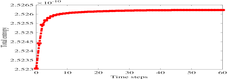
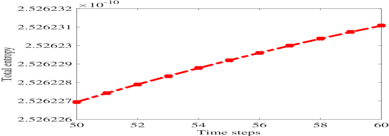
Fig. 1: Example 1: the total entropy profile with time steps.

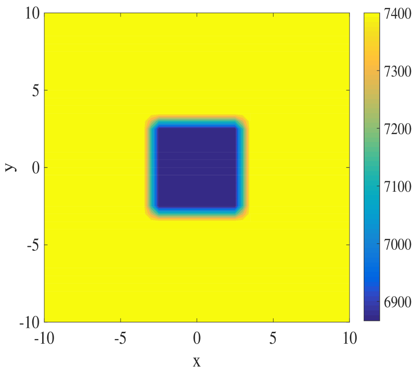
(a) C₁ at the initial time

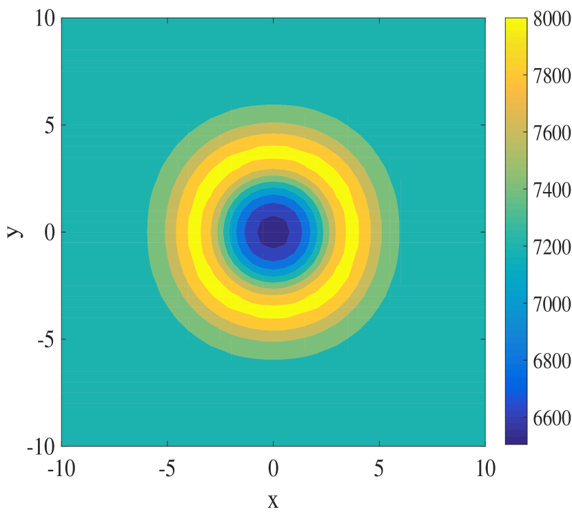
(b) C₁ at the 30th time step

(c) C₁ at the 60th time step

Fig. 2: Example 1: molar densities of C₁ at different time steps.

(a) C₅ at the the initial time

(b) C₅ at the 30th time step

(c) C₅ at the 60th time step

Fig. 3: Example 1: molar densities of C₅ at different time steps.

(a) $T$ at the10th time step

(b) $T$ at the 30th time step

(c) $T$ at the 60th time step

Fig. 4: Example 1: temperature ($T$) contours at different time steps.

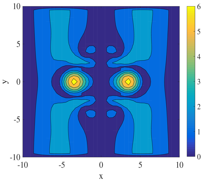
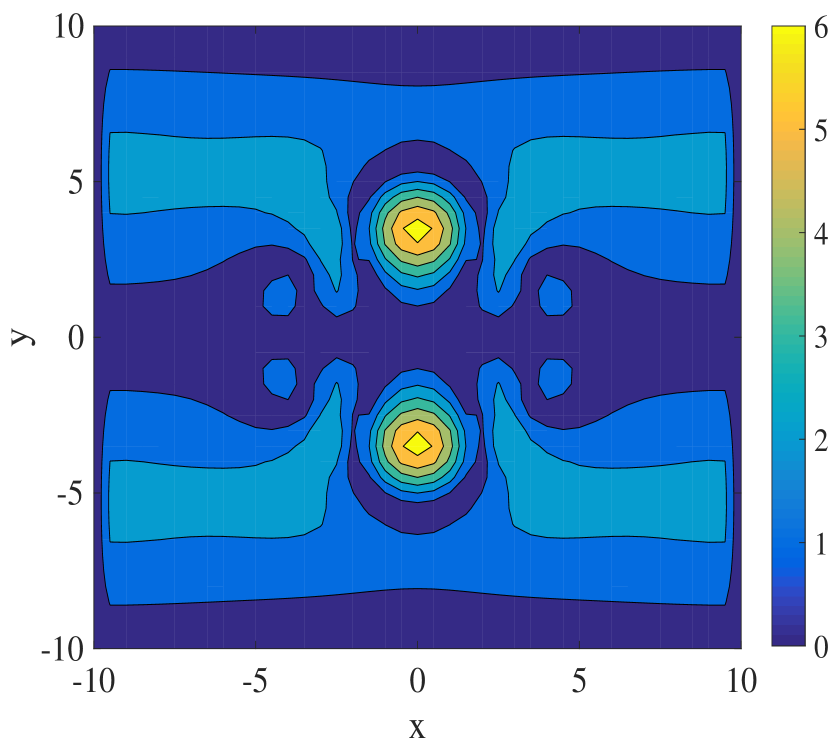
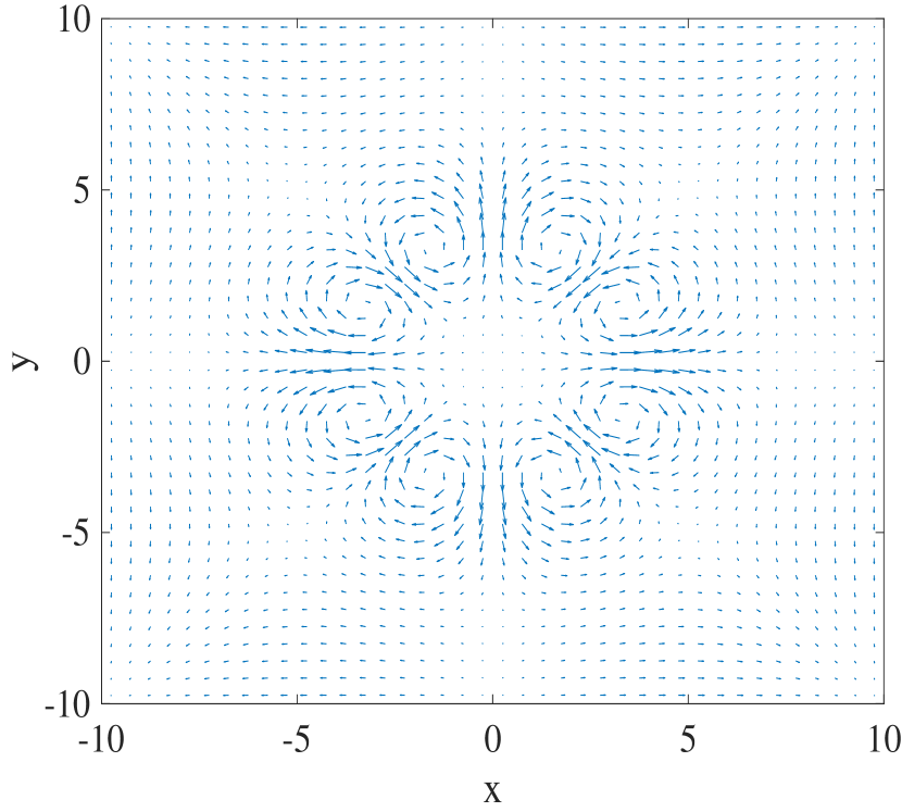
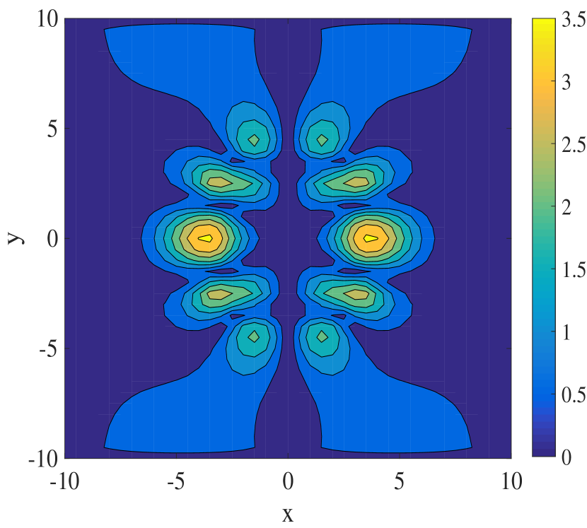
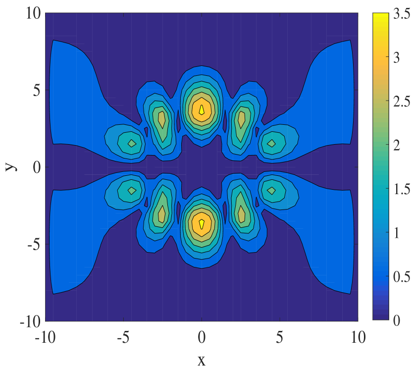
Fig. 5: Example 1: flow quivers (left column), magnitude contours of $x$-direction velocity component (center column), and magnitude contours of $y$-direction velocity component (right column) at the 30th(top row) and 60th(bottom row) time step respectively.

6 Conclusions

A general model obeying the thermodynamic laws and Onsager’s reciprocal relations and characterizing compressibility and partial miscibility between multiple fluids has been developed for non-isothermal multi-component diffuse-interface two-phase flows with realistic equations of state. This model is formulised by a set of nonlinear and coupling equations, including the component mass balance equations, the momentum conservation equation and the total energy balance equation, which is unified for general reference velocities. We have proved an important relation between pressure, chemical potential and temperature, and on the basis of it, we obtain a new formulation of the momentum conservation equation, which indicates that the gradients of chemical potentials and temperature become the primary driving force of the fluid motion except for the external forces. For numerical simulations, we have proposed an efficient, entropy stable numerical method based on the convex-concave splitting of Helmholtz free energy density with respect to molar densities and temperature. We have proved unconditional entropy stability of the proposed method by deriving the variations of Helmholtz free energy and kinetic energy with time steps. Numerical results are provided to validate the proposed method.

Appendix A Helmholtz free energy density

We describe the computations of Helmholtz free energy density $f_{b}({\bm{n}},T)$ of a homogeneous fluid determined by Peng-Robinson equation of state [54].

Let $R$ be the universal gas constant. We denote by $T_{c_{i}}$ and $P_{c_{i}}$ the $i$th component critical temperature and critical pressure, respectively. For the $i$th component, let the reduced temperature be $T_{r_{i}}=T/T_{c_{i}}$. We let the mole fraction of component $i$ be $y_{i}=n_{i}/n$, where $n=\sum_{i=1}^{M}n_{i}$ is the overall molar density. The parameters $a_{i}$ and $b_{i}$ are calculated as

$$a_{i}=0.45724\frac{R^{2}T_{c_{i}}^{2}}{P_{c_{i}}}\left[1+m_{i}(1-\sqrt{T_{r_{i}}})\right]^{2},~{}~{}~{}~{}b_{i}=0.07780\frac{RT_{c_{i}}}{P_{c_{i}}}.$$ (A.1)

The coefficients $m_{i}$ are calculated by the following formulas

$$m_{i}=0.37464+1.54226\omega_{i}-0.26992\omega_{i}^{2},~{}~{}\omega_{i}\leq 0.49,$$ (A.2a)

$$m_{i}=0.379642+1.485030\omega_{i}-0.164423\omega_{i}^{2}+0.016666\omega_{i}^{3},~{}~{}\omega_{i}>0.49,$$ (A.2b)

where $\omega_{i}$ is the acentric factor. Finally, $a(T)$ and $b$ are calculated by

$$a=\sum_{i=1}^{M}\sum_{j=1}^{M}y_{i}y_{j}\left(a_{i}a_{j}\right)^{1/2}(1-k_{ij}),~{}~{}~{}~{}b=\sum_{i=1}^{M}y_{i}b_{i},$$ (A.3)

where $k_{ij}$ the given binary interaction coefficients for the energy parameters.

The correlation coefficients $\alpha_{ik}$ estimate the molar heat capacity of ideal gas at the constant pressure as

$$\psi_{i}^{p}(T)=\sum_{k=0}^{3}\alpha_{ik}T^{k}.$$ (A.4)

We list the correlation coefficients of methane and pentane in Table 2.

The bulk Helmholtz free energy density, denoted by $f_{b}$, is calculated as a sum of three contributions

$$f_{b}(n,T) = f_{b}^{\textnormal{ideal}}(n,T)+f_{b}^{\textnormal{repulsion}}(n,T)+f_{b}^{\textnormal{attraction}}(n,T),$$ (A.5)

where

$$f_{b}^{\textnormal{ideal}}(n,T) = n\vartheta_{0}-ns_{0}T+\sum_{i=1}^{M}n_{i}\sum_{k=0}^{3}\alpha_{ik}\frac{T^{k+1}-T_{0}^{k+1}}{k+1}-nR(T-T_{0})$$ (A.6)

$$-\sum_{i=1}^{M}n_{i}RT\ln\left(\frac{P_{0}}{n_{i}RT}\right)-\sum_{i=1}^{M}n_{i}T\int_{T_{0}}^{T}\frac{\psi_{i}^{p}(\xi)}{\xi}d\xi,$$

$$f_{b}^{\textnormal{repulsion}}(n,T)=-nRT\ln\left(1-bn\right),$$ (A.7)

$$f_{b}^{\textnormal{attraction}}(n,T)=\frac{a(T)n}{2\sqrt{2}b}\ln\left(\frac{1+(1-\sqrt{2})bn}{1+(1+\sqrt{2})bn}\right),$$ (A.8)

where $T_{0}=298.15$K, $P_{0}=1$bar, $\vartheta_{0}=-2478.95687512$ J$/$mol and $s_{0}=59.5827$ J$/($mol$\cdot$K) for the mixture of methane and pentane in numerical tests.

Appendix B Internal energy and entropy

The bulk internal energy, denoted by $\vartheta_{b}$, is formulated as

$$\vartheta_{b}(n,T) = n\vartheta_{0}+\sum_{i=1}^{M}n_{i}\sum_{k=0}^{3}\alpha_{ik}\frac{T^{k+1}-T_{0}^{k+1}}{k+1}-nR(T-T_{0})$$ (B.1)

$$+\frac{n\left(a(T)-Ta^{\prime}(T)\right)}{2\sqrt{2}b}\ln\left(\frac{1+(1-\sqrt{2})bn}{1+(1+\sqrt{2})bn}\right),$$

where $a^{\prime}(T)$ denotes the derivative with respect to $T$. We denote by $s_{b}$ the bulk entropy and express it as

$$s_{b}(n,T) = ns_{0}+nR\ln\left(1-bn\right)+\sum_{i=1}^{M}n_{i}R\ln\left(\frac{P_{0}}{n_{i}RT}\right)+\sum_{i=1}^{M}n_{i}\int_{T_{0}}^{T}\frac{\psi^{p}_{i}(\xi)}{\xi}d\xi$$ (B.2)

$$-\frac{na^{\prime}(T)}{2\sqrt{2}b}\ln\left(\frac{1+(1-\sqrt{2})bn}{1+(1+\sqrt{2})bn}\right).$$

The above formulations are referred to [60].

Appendix C Some physical parameters

The influence parameters in numerical tests are taken as

$$\bm{c}=(c_{ij})_{i,j=1}^{2}=\left(\begin{array}[]{cc}0.0282&0.0462\\ 0.0462&0.3019\end{array}\right)\times 1e-18.$$

We list some physical parameters of the substances in Tables 1, 2 and 3.

Table 1: Physical parameters

Substance	$P_{c}$(bar)	$T_{c}$(K)	Acentric factor	$M_{w}$(g/mole)
methane	45.99	190.56	0.011	16.04
pentane	33.70	469.7	0.251	72.15

Table 2: The correlation coefficients in the heat capacity

Substance	$\alpha_{0}$	$\alpha_{1}$	$\alpha_{2}$	$\alpha_{3}$
methane	19.25	5.213e-2	1.197e-5	-1.132e-8
pentane	-3.626	4.873e-1	-2.580e-4	5.305e-8

Table 3: Binary interaction coefficients

	methane	pentane
methane	0	0.041
pentane	0.041	0

References

• [1] H. Abels, H. Garcke, G. Grün. Thermodynamically consistent, frame indifferent diffuse interface models for incompressible two-phase flows with different densities. Mathematical Models and Methods in Applied Sciences, Vol. 22, No. 3, 1150013, 2012.
• [2] F. O. Alpak, B. Riviere, F. Frank. A phase-field method for the direct simulation of two-phase flows in pore-scale media using a non-equilibrium wetting boundary condition. Computational Geosciences, 20: 881–908, 2016.
• [3] D. M. Anderson, G. B. McFadden, A. A. Wheeler. Diffuse-Interface Methods in Fluid Mechanics. Annual Review of Fluid Mechanics, 30: 139-165, 1998.
• [4] T. Arbogast, M.F. Wheeler, I. Yotov. Mixed finite elements for elliptic problems with tensor coefficients as cell-centered finite differences. SIAM Journal on Numerical Analysis, 4(2): 828–852, 1997.
• [5] K. Bao, Y. Shi, S. Sun, X.-P. Wang. A finite element method for the numerical solution of the coupled Cahn-Hilliard and Navier-Stokes system for moving contact line problems. Journal of Computational Physics, 231(24): 8083–8099, 2012.
• [6] A. Baskaran, J. Lowengrub, C. Wang, S. Wise. Convergence analysis of a second order convex splitting scheme for the modified phase field crystal equation. SIAM Journal on Numerical Analysis, 51(5): 2851–2873, 2013.
• [7] F. Boyer, C. Lapuerta. Study of a three component Cahn-Hilliard flow model. ESAIM: Mathematical Modelling and Numerical Analysis, 40(4): 653–687, 2006.
• [8] J. Bueno, H. Gomez. Liquid-vapor transformations with surfactants. Phase-field model and Isogeometric Analysis. Journal of Computational Physics, 321: 797–818, 2016.
• [9] J. W. Cahn, J. E. Hilliard. Free Energy of a Nonuniform System. I. Interfacial Free Energy. Journal of Chemical Physics, 28: 258-267, 1958.
• [10] A. Chaudhri, J. B. Bell, A. L. Garcia, A. Donev. Modeling multiphase flow using fluctuating hydrodynamics. Physical Review E, 90, 033014, 2014.
• [11] Z. Chen, G. Huan, Y. Ma, Computational methods for multiphase flows in porous media. SIAM Comp. Sci. Eng., Philadelphia, 2006.
• [12] Y. Chen, J. Shen. Efficient, adaptive energy stable schemes for the incompressible Cahn-Hilliard Navier-Stokes phase-field models. Journal of Computational Physics, 308: 40-56, 2016.
• [13] S. R. De Groot, P. Mazur. Non-Equilibrium Thermodynamics. Dover Publications, New York, 2011.
• [14] H. Ding, P.D.M. Spelt, C. Shu. Diffuse interface model for incompressible two-phase flows with large density ratios. Journal of Computational Physics, 226: 2078–2095, 2007.
• [15] S. Dong. Wall-bounded multiphase flows of N immiscible incompressible fluids: Consistency and contact-angle boundary condition. Journal of Computational Physics, 338: 21–67, 2017.
• [16] C. M. Elliott, A. M. Stuart, The global dynamics of discrete semilinear parabolic equations, SIAM Journal on Numerical Analysis, 30: 1622–1663, 1993.
• [17] H. Emmerich. The Diffuse Interface Approach in Materials Science: Thermodynamic Concepts and Applications of Phase-Field Models. Springer, 2011.
• [18] D. J. Eyre. Unconditionally gradient stable time marching the Cahn-Hilliard equation. Computational and mathematical models of microstructural evolution (San Francisco, CA, 1998), Mater. Res. Soc. Sympos. Proc., 529: 39–46. MRS, Warrendale, PA, 1998.
• [19] X. Fan, J. Kou, Z. Qiao, S. Sun. A Componentwise Convex Splitting Scheme for Diffuse Interface Models with Van der Waals and Peng–Robinson Equations of State. SIAM Journal on Scientific Computing, 39(1): B1–B28, 2017.
• [20] A. Firoozabadi. Thermodynamics of hydrocarbon reservoirs. McGraw-Hill New York, 1999.
• [21] V. Girault, H. Lopez. Finite-element error estimates for the MAC scheme. IMA Journal of Numerical Analysis, 16(3): 347-379, 1996.
• [22] G. Gonnella, A. Lamura, A. Piscitelli. Dynamics of binary mixtures in inhomogeneous temperatures. Journal of Physics A: Mathematical and Theoretical, 41, 105001, 2008.
• [23] Z. Guo, P. Lin A thermodynamically consistent phase-field model for two-phase flows with thermocapillary effects. Journal of Fluid Mechanics, 766: 226–271, 2015.
• [24] J. Guo, C. Wang, S. Wise, X. Yue. An $H^{2}$ convergence of a second-order convex-splitting, finite difference scheme for the three-dimensional Cahn-Hilliard equation. Communications in Mathematical Sciences, 14: 489-515, 2016.
• [25] H. Hoteit. Modeling diffusion and gas-oil mass transfer in fractured reservoirs. Journal of Petroleum Science and Engineering, 105: 1–17, 2013.
• [26] T. Jindrová, J. Miky$\check{\textnormal{s}}$ka. Fast and robust algorithm for calculation of two-phase equilibria at given volume, temperature, and moles. Fluid Phase Equilibria, 353: 101–114, 2013.
• [27] T. Jindrová, J. Miky$\check{\textnormal{s}}$ka. General algorithm for multiphase equilibria calculation at given volume, temperature, and moles. Fluid Phase Equilibria, 393: 7–25, 2015.
• [28] J. Kim. A generalized continuous surface tension force formulation for phase-field models for multi-component immiscible fluid flows. Computer Methods in Applied Mechanics and Engineering, 198: 3105–3112, 2009.
• [29] J. Kim. Phase-field models for multi-component fluid flows. Communications in Computational Physics, 2(3): 613–661, 2012.
• [30] J. Kou, S. Sun, X. Wang. Efficient numerical methods for simulating surface tension of multi-component mixtures with the gradient theory of fluid interfaces. Computer Methods in Applied Mechanics and Engineering, 292: 92–106, 2015.
• [31] J. Kou, S. Sun. Numerical methods for a multi-component two-phase interface model with geometric mean influence parameters. SIAM Journal on Scientific Computing, 37(4): B543–B569, 2015.
• [32] J. Kou, S. Sun. Unconditionally stable methods for simulating multi-component two-phase interface models with Peng-Robinson equation of state and various boundary conditions. Journal of Computational and Applied Mathematics, 291(1): 158–182, 2016.
• [33] J. Kou, S. Sun, X. Wang. An energy stable evolution method for simulating two-phase equilibria of multi-component fluids at constant moles, volume and temperature. Computational Geosciences, 20: 283–295, 2016.
• [34] J. Kou, S. Sun. Multi-scale diffuse interface modeling of multi-component two-phase flow with partial miscibility. Journal of Computational Physics, 318: 349–372, 2016.
• [35] J. Kou, S. Sun. Thermodynamically consistent modeling and simulation of multi-component two-phase flow with partial miscibility. Computer Methods in Applied Mechanics and Engineering, 331: 623–649, 2018.
• [36] J. Kou, S. Sun. A stable algorithm for calculating phase equilibria with capillarity at specified moles, volume and temperature using a dynamic model. Fluid Phase Equilibria, 456: 7–24, 2018.
• [37] J. Kou, S. Sun. Thermodynamically consistent simulation of nonisothermal diffuse-interface two-phase flow with Peng-Robinson equation of state, arXiv:1712.03090 [math.NA], 2017.
• [38] Z. Li, B. C.-Y. Lu. On the prediction of surface tension for multicomponent mixtures. The Canadian Journal of Chemical Engineering, 79(3): 402–411, 2001.
• [39] H. Li, L. Ju, C. Zhang, Q. Peng. Unconditionally energy stable linear schemes for the diffuse interface model with Peng-Robinson equation of state. Journal of Scientific Computing, DOI 10.1007/s10915-017-0576-7, 2017.
• [40] Y. Li, J.-I. Choi, J. Kim. Multi-component Cahn-Hilliard system with different boundary conditions in complex domains. Journal of Computational Physics, 323: 1–16, 2016.
• [41] Y. Li, J. Kou, S. Sun. Numerical modeling of isothermal compositional grading by convex splitting methods. Journal of Natural Gas Science and Engineering, 43: 207–221, 2017.
• [42] J. Liu, C. M. Landis, H. Gomez, T. J.R. Hughes. Liquid–vapor phase transition: Thermomechanical theory, entropy stable numerical formulation, and boiling simulations. Computer Methods in Applied Mechanics and Engineering, 297: 476–553, 2015.
• [43] J. Liu, G. Amberg, M. Do-Quang. Diffuse interface method for a compressible binary fluid. Physical Review E, 93, 013121, 2016.
• [44] A. Leahy-Dios, A. Firoozabadi. Unified Model for Nonideal Multicomponent Molecular Diffusion Coefficients. AIChE Journal, 53(11): 2932–2939, 2007.
• [45] J. Miky$\check{\textnormal{s}}$ka, A. Firoozabadi. A new thermodynamic function for phase-splitting at constant temperature, moles, and volume. AIChE Journal, 57(7):1897–1904, 2011.
• [46] J. Miky$\check{\textnormal{s}}$ka, A. Firoozabadi. Investigation of mixture stability at given volume, temperature, and number of moles. Fluid Phase Equilibria, 321:1–9, 2012.
• [47] C. Miqueu, B. Mendiboure, C. Graciaa, J. Lachaise. Modelling of the surface tension of binary and ternary mixtures with the gradient theory of fluid interfaces. Fluid Phase Equilibria, 218: 189–203, 2004.
• [48] J. Moortgat, A. Firoozabadi. Higher-order compositional modeling of three-phase flow in 3D fractured porous media based on cross-flow equilibrium. Journal of Computational Physics, 250: 425–445, 2013.
• [49] N.R. Nagarajan, A.S. Cullick. New strategy for phase equilibrium and critical point calculations by thermodynamic energy analysis. Part I. Stability analysis and flash. Fluid Phase Equilibria, 62(3): 191–210, 1991.
• [50] A. Onuki. Dynamic van der Waals theory of two-phase fluids in heat flow. Physical Review Letters, 94(5): 054501, 2005.
• [51] A. Onuki. Dynamic van der Waals theory. Physical Review E, 75(3): 036304, 2007.
• [52] A. Pecenko, J.G.M. Kuerten, C.W.M. van der Geld. A diffuse-interface approach to two-phase isothermal flow of a Van der Waals fluid near the critical point, International Journal of Multiphase Flow, 36: 558–569, 2010.
• [53] A. Pecenko, L.G.M. van Deurzen, J.G.M. Kuerten, C.W.M. van der Geld. Non-isothermal two-phase flow with a diffuse-interface model. International Journal of Multiphase Flow, 37: 149-165, 2011.
• [54] D. Peng, D.B. Robinson. A new two-constant equation of state. Industrial and Engineering Chemistry Fundamentals, 15(1): 59–64, 1976.
• [55] Q. Peng. A convex-splitting scheme for a diffuse interface model with Peng-Robinson equation of state. Advances in Applied Mathematics and Mechanics, 9(5): 1162–1188, 2017.
• [56] O. Polívka, J. Miky$\check{\textnormal{s}}$ka. Compositional modeling in porous media using constant volume flash and flux computation without the need for phase identification. Journal of Computational Physics, 272:149–169, 2014.
• [57] Z. Qiao, S. Sun. Two-phase fluid simulation using a diffuse interface model with Peng-Robinson equation of state. SIAM Journal on Scientific Computing, 36(4): B708–B728, 2014.
• [58] A. Rasheed, A. Belmiloudi. Mathematical modelling and numerical simulation of dendrite growth using phase-field method with a magnetic field effect. Communications in Computational Physics, 14: 477–508, 2013.
• [59] J. Shen, X. Yang. Decoupled, energy stable schemes for phase-field models of two-phase incompressible flows. SIAM Journal on Numerical Analysis, 53(1): 279-296, 2015.
• [60] T. Smejkal, J. Miky$\check{\textnormal{s}}$ka. Phase stability testing and phase equilibrium calculation at specified internal energy, volume, and moles. Fluid Phase Equilibria, 431: 82–96, 2017.
• [61] M. T. Taylor, T. Qian. Thermal singularity and contact line motion in pool boiling: Effects of substrate wettability. Physical Review E, 93(3), 033105, 2016.
• [62] G. Tryggvason, R. Scardovelli, S. Zaleski. Direct Numerical Simulations of Gas-Liquid Multiphase Flows. Cambridge University Press, New York, 2011.
• [63] S. M. Wise, C. Wang, J. S. Lowengrub. An energy-stable and convergent finite-difference scheme for the phase field crystal equation. SIAM Journal on Numerical Analysis, 47(3): 2269–2288, 2009.
• [64] X. Yang, J. Zhao, Q. Wang, J. Shen. Numerical approximations for a three-component Cahn-Hilliard phase-field model based on the invariant energy quadratization method. Mathematical Models and Methods in Applied Sciences, 27(11): 1993–2030, 2017.
• [65] Q. Zhang, X.-P. Wang. Phase field modeling and simulation of three-phase flow on solid surfaces. Journal of Computational Physics, 319: 79–107, 2016.