Active Learning with Logged Data

Abstract

We consider active learning with logged data, where labeled examples are drawn conditioned on a predetermined logging policy, and the goal is to learn a classifier on the entire population, not just conditioned on the logging policy. Prior work addresses this problem either when only logged data is available, or purely in a controlled random experimentation setting where the logged data is ignored. In this work, we combine both approaches to provide an algorithm that uses logged data to bootstrap and inform experimentation, thus achieving the best of both worlds. Our work is inspired by a connection between controlled random experimentation and active learning, and modifies existing disagreement-based active learning algorithms to exploit logged data.

1 Introduction

We consider learning a classifier from logged data. Here, the learner has access to a logged labeled dataset that has been collected according to a known pre-determined policy, and his goal is to learn a classifier that predicts the labels accurately over the entire population, not just conditioned on the logging policy.

This problem arises frequently in many natural settings. An example is predicting the efficacy of a treatment as a function of patient characteristics based on observed data. Doctors may assign the treatment to patients based on some predetermined rule; recording these patient outcomes produces a logged dataset where outcomes are observed conditioned on the doctors’ assignment. A second example is recidivism prediction, where the goal is to predict whether a convict will re-offend. Judges use their own predefined policy to grant parole, and if parole is granted, then an outcome (reoffense or not) is observed. Thus the observed data records outcomes conditioned on the judges’ parole policy, while the learner’s goal is to learn a predictor over the entire population.

A major challenge in learning from logged data is that the logging policy may leave large areas of the data distribution under-explored. Consequently, empirical risk minimization (ERM) on the logged data leads to classifiers that may be highly suboptimal on the population. When the logging policy is known, a second option is to use a weighted ERM, that reweighs each observed labeled data point to ensure that it reflects the underlying population. However, this may lead to sample inefficiency if the logging policy does not adequately explore essential regions of the population. A final approach, typically used in clinical trials, is controlled random experimentation – essentially, ignore the logged data, and record outcomes for fresh examples drawn from the population. This approach is expensive due to the high cost of trials, and wasteful since it ignores the observed data.

Motivated by these challenges, we propose active learning to combine logged data with a small amount of strategically chosen labeled data that can be used to correct the bias in the logging policy. This solution has the potential to achieve the best of both worlds by limiting experimentation to achieve higher sample efficiency, and by making the most of the logged data. Specifically, we assume that in addition to the logged data, the learner has some additional unlabeled data that he can selectively ask an annotator to label. The learner’s goal is to learn a highly accurate classifier over the entire population by using a combination of the logged data and with as few label queries to the annotator as possible.

How can we utilize logged data for better active learning? This problem has not been studied to the best of our knowledge. A naive approach is to use the logged data to come up with a warm start and then do standard active learning. In this work, we show that we can do even better. In addition to the warm start, we show how to use multiple importance sampling estimators to utilize the logged data more efficiently. Additionally, we introduce a novel debiasing policy that selectively avoids label queries for those examples that are highly represented in the logged data.

Combining these three approaches, we provide a new algorithm. We prove that our algorithm is statistically consistent, and has a lower label requirement than simple active learning that uses the logged data as a warm start. Finally, we evaluate our algorithm experimentally on various datasets and logging policies. Our experiments show that the performance of our method is either the best or close to the best for a variety of datasets and logging policies. This confirms that active learning to combine logged data with carefully chosen labeled data may indeed yield performance gains.

2 Preliminaries

2.1 Problem Setup

Instances are drawn from an instance space $\mathcal{X}$ and a label space $\mathcal{Y}=\{0,1\}$. There is an underlying data distribution $D$ over $\mathcal{X}\times\mathcal{Y}$ that describes the population. There is a hypothesis space $\mathcal{H}\subset\mathcal{Y}^{\mathcal{X}}$. For simplicity, we assume $\mathcal{H}$ is a finite set, but our results can be generalized to VC-classes by standard arguments (Vapnik & Chervonenkis, 1971).

The learning algorithm has access to two sources of data: logged data, and online data. The logged data are generated from $m$ examples $\{(X_{t},Y_{t})\}_{t=1}^{m}$ drawn i.i.d. from $D$, and a logging policy $Q_{0}:\mathcal{X}\rightarrow[0,1]$ that determines the probability of observing the label. For each example $(X_{t},Y_{t})$ ($1\leq t\leq m$), an independent Bernoulli random variable $Z_{t}$ is drawn with expectation $Q_{0}(X_{t})$, and then the label $Y_{t}$ is revealed to the learning algorithm if $Z_{t}=1$. We call $T_{0}=\{(X_{t},Y_{t},Z_{t})\}_{t=1}^{m}$ the logged dataset. From the algorithm’s perspective, we assume it knows the logging policy $Q_{0}$, and only observes instances $\{X_{t}\}_{t=1}^{m}$, decisions of the policy $\{Z_{t}\}_{t=1}^{m}$, and revealed labels $\{Y_{t}\mid Z_{t}=1\}_{t=1}^{m}$.

The online data are generated as follows. Suppose there is a stream of another $n$ examples $\{(X_{t},Y_{t})\}_{t=m+1}^{m+n}$ drawn i.i.d. from distribution $D$. At time $t$ ($m<t\leq m+n$), the algorithm uses its query policy to compute a bit $Z_{t}\in\{0,1\}$, and then the label $Y_{t}$ is revealed to the algorithm if $Z_{t}=1$. The computation of $Z_{t}$ may in general be randomized, and is based on the observed logged data $T_{0}$, observed instances $\{X_{i}\}_{i=m+1}^{t}$, previous decisions$\{Z_{i}\}_{i=m+1}^{t-1}$, and observed labels $\{Y_{i}\mid Z_{i}=1\}_{i=m+1}^{t-1}$.

The goal of the algorithm is to learn a classifier $h\in\mathcal{H}$ from observed logged data and online data. Fixing $D$, $Q_{0}$, $m$, $n$, the performance measures are: (1) the error rate $l(h):=\Pr_{D}(h(X)\neq Y)$ of the output classifier, and (2) the number of label queries on the online data. Note that the error rate is over the entire population $D$ instead of conditioned on the logging policy, and that we assume the logged data $T_{0}$ come at no cost. In this work, we are interested in the situation where $n$ is about the same as or less than $m$.

2.2 Background on Disagreement-Based Active Learning

Our algorithm is based on Disagreement-Based Active Learning (DBAL) which has rigorous theoretical guarantees and can be implemented practically (see (Hanneke et al., 2014) for a survey, and (Hanneke & Yang, 2015; Huang et al., 2015) for some recent developments). DBAL iteratively maintains a candidate set of classifiers that contains the optimal classifier $h^{\star}:=\arg\min_{h\in\mathcal{H}}l(h)$ with high probability. At the $k$-th iteration, the candidate set $V_{k}$ is constructed as all classifiers which have low estimated error on examples observed up to round $k$. Based on $V_{k}$, the algorithm constructs a disagreement set $D_{k}$ to be a set of instances on which there are at least two classifiers in $V_{k}$ that predict different labels. Then the algorithm draws a set $T_{k}$ of unlabeled examples, where the size of $T_{k}$ is a parameter of the algorithm. For each instance $X\in T_{k}$, if it falls into the disagreement region $D_{k}$, then the algorithm queries for its label; otherwise, observing that all classifiers in $V_{k}$ have the same prediction on $X$, its label is not queried. The queried labels are then used to update future candidate sets.

2.3 Background on Error Estimators

Most learning algorithms, including DBAL, require estimating the error rate of a classifier. A good error estimator should be unbiased and of low variance. When instances are observed with different probabilities, a commonly used error estimator is the standard importance sampling estimator that reweighs each observed labeled example according to the inverse probability of observing it.

Consider a simplified setting where the logged dataset $T_{0}=(X_{i},Y_{i},Z_{i})_{i=1}^{m}$ and $\Pr(Z_{i}=1\mid X_{i})=Q_{0}(X_{i})$. On the online dataset $T_{1}=(X_{i},Y_{i},Z_{i})_{i=m+1}^{m+n}$, the algorithm uses a fixed query policy $Q_{1}$ to determine whether to query for labels, that is, $\Pr(Z_{i}=1\mid X_{i})=Q_{1}(X_{i})$ for $m<i\leq m+n$. Let $S=T_{0}\cup T_{1}$.

In this setting, the standard importance sampling (IS) error estimator for a classifier $h$ is:

$$l_{\text{IS}}(h,S):= \frac{1}{m+n}\sum_{i=1}^{m}\frac{\mathds{1}\{h(X_{i})\neq Y_{i}\}Z_{i}}{Q_{0}(X_{i})}$$

$$+\frac{1}{m+n}\sum_{i=m+1}^{m+n}\frac{\mathds{1}\{h(X_{i})\neq Y_{i}\}Z_{i}}{Q_{1}(X_{i})}.$$ (1)

$l_{\text{IS}}$ is unbiased, and its variance is proportional to $\sup_{i=0,1;x\in\mathcal{X}}\frac{1}{Q_{i}(x)}$. Although the learning algorithm can choose its query policy $Q_{1}$ to avoid $Q_{1}(X_{i})$ to be too small for $i>m$, $Q_{0}$ is the logging policy that cannot be changed. When $Q_{0}(X_{i})$ is small for some $i\leq m$, the estimator in (1) have a high variance such that it may be even better to just ignore the logged dataset $T_{0}$.

An alternative is the multiple importance sampling (MIS) estimator with balanced heuristic (Veach & Guibas, 1995):

$$l_{\text{MIS}}(h,S):=\sum_{i=1}^{m+n}\frac{\mathds{1}\{h(X_{i})\neq Y_{i}\}Z_{i}}{mQ_{0}(X_{i})+nQ_{1}(X_{i})}.$$ (2)

It can be proved that $l_{\text{MIS}}(h,S)$ is indeed an unbiased estimator for $l(h)$. Moreover, as proved in (Owen & Zhou, 2000; Agarwal et al., 2017), (2) always has a lower variance than both (1) and the standard importance sampling estimator that ignores the logged data.

In this paper, we use multiple importance sampling estimators, and write $l_{\text{MIS}}(h,S)$ as $l(h,S)$.

Additional Notations

In this paper, unless otherwise specified, all probabilities and expectations are over the distribution $D$, and we drop $D$ from subscripts henceforth.

Let $\rho(h_{1},h_{2}):=\Pr(h_{1}(X)\neq h_{2}(X))$ be the disagreement mass between $h_{1}$ and $h_{2}$, and $\rho_{S}(h_{1},h_{2}):=\frac{1}{N}\sum_{i=1}^{N}\mathds{1}\{h_{1}(x_{i})\neq h_{2}(x_{i})\}$ for $S=\{x_{1},x_{2},\dots,x_{N}\}\subset\mathcal{X}$ be the empirical disagreement mass between $h_{1}$ and $h_{2}$ on $S$.

For any $h\in\mathcal{H}$, $r>0$, define $B(h,r):=\{h^{\prime}\in\mathcal{H}\mid\rho(h,h^{\prime})\leq r\}$ to be $r$-ball around $h$. For any $V\subseteq\mathcal{H}$, define the disagreement region $\text{DIS}(V):=\{x\in\mathcal{X}\mid\exists h_{1}\neq h_{2}\in V\text{ s.t. }h_{1}(x)\neq h_{2}(x)\}$.

3 Algorithm

3.1 Main Ideas

Our algorithm employs the disagreement-based active learning framework, but modifies the main DBAL algorithm in three key ways.

Key Idea 1: Warm-Start

Our algorithm applies a straightforward way of making use of the logged data $T_{0}$ inside the DBAL framework: to set the initial candidate set $V_{0}$ to be the set of classifiers that have a low empirical error on $T_{0}$.

Key Idea 2: Multiple Importance Sampling

Our algorithm uses multiple importance sampling estimators instead of standard importance sampling estimators. As noted in the previous section, in our setting, multiple importance sampling estimators are unbiased and have lower variance, which results in a better performance guarantee.

We remark that the main purpose of using multiple importance sampling estimators here is to control the variance due to the predetermined logging policy. In the classical active learning setting without logged data, standard importance sampling can give satisfactory performance guarantees (Beygelzimer et al., 2009, 2010; Huang et al., 2015).

Key Idea 3: A Debiasing Query Strategy

The logging policy $Q_{0}$ introduces bias into the logged data: some examples may be underrepresented since $Q_{0}$ chooses to reveal their labels with lower probability. Our algorithm employs a debiasing query strategy to neutralize this effect. For any instance $x$ in the online data, the algorithm would query for its label with a lower probability if $Q_{0}(x)$ is relatively large.

It is clear that a lower query probability leads to fewer label queries. Moreover, we claim that our debiasing strategy, though queries for less labels, does not deteriorate our theoretical guarantee on the error rate of the final output classifier. To see this, we note that we can establish a concentration bound for multiple importance sampling estimators that with probability at least $1-\delta$, for all $h\in\mathcal{H}$,

$$l(h)-l(h^{\star})\leq 2(l(h,S)-l(h^{\star},S))$$

$$+ \gamma_{1}\sup_{x\in\mathcal{X}}\frac{\mathds{1}\{h(x)\neq h^{\star}(x)\}\log\frac{|\mathcal{H}|}{\delta}}{mQ_{0}(x)+nQ_{1}(x)}$$

$$+ \gamma_{1}\sqrt{\sup_{x\in\mathcal{X}}\frac{\mathds{1}\{h(x)\neq h^{\star}(x)\}\log\frac{|\mathcal{H}|}{\delta}}{mQ_{0}(x)+nQ_{1}(x)}l(h^{\star})}$$ (3)

where $m,n$ are sizes of logged data and online data respectively, $Q_{0}$ and $Q_{1}$ are query policy during the logging phase and the online phase respectively, and $\gamma_{1}$ is an absolute constant (see Corollary 15 in Appendix for proof).

This concentration bound implies that for any $x\in\mathcal{X}$, if $Q_{0}(x)$ is large, we can set $Q_{1}(x)$ to be relatively small (as long as $mQ_{0}(x)+nQ_{1}(x)\geq\inf_{x^{\prime}}mQ_{0}(x^{\prime})+nQ_{1}(x^{\prime})$) while achieving the same concentration bound. Consequently, the upper bound on the final error rate that we can establish from this concentration bound would not be impacted by the debiasing querying strategy.

One technical difficulty of applying both multiple importance sampling and the debiasing strategy to the DBAL framework is adaptivity. Applying both methods requires that the query policy and consequently the importance weights in the error estimator are updated with observed examples in each iteration. In this case, the summands of the error estimator are not independent, and the estimator becomes an adaptive multiple importance sampling estimator whose convergence property is still an open problem (Cornuet et al., 2012).

To circumvent this convergence issue and establish rigorous theoretical guarantees, in each iteration, we compute the error estimator from a fresh sample set. In particular, we partition the logged data and the online data stream into disjoint subsets, and we use one logged subset and one online subset for each iteration.

3.2 Details of the Algorithm

1:  Input: confidence $\delta$, size of online data $n$, logging policy $Q_{0}$, logged data $T_{0}$.

2:  $K\leftarrow\lceil\log{n}\rceil$.

3:  $\tilde{S}_{0}\leftarrow T_{0}^{(0)}$; $V_{0}\leftarrow\mathcal{H}$; $D_{0}\leftarrow\mathcal{X}$; $\xi_{0}\leftarrow\inf_{x\in\mathcal{X}}Q_{0}(x)$.

4:  for $k=0,\dots,K-1$ do

5:     Define $\delta_{k}\leftarrow\frac{\delta}{(k+1)(k+2)}$; $\sigma(k,\delta)\leftarrow\frac{\log|\mathcal{H}|/\delta}{m_{k}\xi_{k}+n_{k}}$; $\Delta_{k}(h,h^{\prime})\leftarrow\gamma_{0}(\sigma(k,\frac{\delta_{k}}{2})+\sqrt{\sigma(k,\frac{\delta_{k}}{2})\rho_{\tilde{S}_{k}}(h,h^{\prime})})$.

6:     $\triangleright$ $\gamma_{0}$ is an absolute constant defined in Lemma 16.

7:     $\hat{h}_{k}\leftarrow\arg\min_{h\in V_{k}}l(h,\tilde{S}_{k})$.

8:     Define the candidate set

$$V_{k+1}\leftarrow\{h\in V_{k}\mid l(h,\tilde{S}_{k})\leq l(\hat{h}_{k},\tilde{S}_{k})+\Delta_{k}(h,\hat{h}_{k})\}$$

and its disagreement region $D_{k+1}\leftarrow\text{DIS}(V_{k+1})$.

9:     Define $\xi_{k+1}\leftarrow\inf_{x\in D_{k+1}}Q_{0}(x)$, and $Q_{k+1}(x)\leftarrow\mathds{1}\{Q_{0}(x)\leq\xi_{k+1}+1/\alpha\}$.

10:     Draw $n_{k+1}$ samples $\{(X_{t},Y_{t})\}_{t=m+n_{1}\cdots+n_{k}+1}^{m+n_{1}+\cdots+n_{k+1}}$, and present $\{X_{t}\}_{t=m+n_{1}+\cdots+n_{k}+1}^{m+n_{1}+\cdots+n_{k+1}}$ to the algorithm.

11:     for $t=m+n_{1}+\cdots+n_{k}+1\text{ to }m+n_{1}+\cdots+n_{k+1}$ do

12:        $Z_{t}\leftarrow Q_{k+1}(X_{t})$.

13:        if $Z_{t}=1$ then

14:           If $X_{t}\in D_{k+1}$, query for label: $\tilde{Y}_{t}\leftarrow Y_{t}$; otherwise infer $\tilde{Y}_{t}\leftarrow\hat{h}_{k}(X_{t})$.

15:        end if

16:     end for

17:     $\tilde{T}_{k+1}\leftarrow\{X_{t},\tilde{Y}_{t},Z_{t}\}_{t=m+n_{1}+\cdots+n_{k}+1}^{m+n_{1}+\cdots+n_{k+1}}$.

18:     $\tilde{S}_{k+1}\leftarrow T_{0}^{(k+1)}\cup\tilde{T}_{k+1}$.

19:  end for

20:  Output $\hat{h}=\arg\min_{h\in V_{K}}l(h,\tilde{S}_{K})$.

Algorithm 1 Acitve learning with logged data

The Algorithm is shown as Algorithm 1. Algorithm 1 runs in $K$ iterations where $K=\lceil\log{n}\rceil$ (recall $n$ is the size of the online data stream). For simplicity, we assume $n=2^{K}-1$.

As noted in the previous subsection, we require the algorithm to use a disjoint sample set for each iteration. Thus, we partition the data as follows. The online data stream is partitioned into $K$ parts $T_{1},\cdots,T_{K}$ of sizes $n_{1}=2^{0},\cdots,n_{K}=2^{K-1}$. We define $n_{0}=0$ for completeness. The logged data $T_{0}$ is partitioned into $K+1$ parts $T_{0}^{(0)},\cdots,T_{0}^{(K)}$ of sizes $m_{0}=m/3,m_{1}=\alpha n_{1},m_{2}=\alpha n_{2},\cdots,m_{K}=\alpha n_{K}$ (where $\alpha=2m/3n$ and we assume $\alpha\geq 1$ is an integer for simplicity. $m_{0}$ can take other values as long as it is a constant factor of $m$). The algorithm uses $T_{0}^{(0)}$ to construct an initial candidate set, and uses $S_{k}:=T_{0}^{(k)}\cup T_{k}$ in iteration $k$.

Algorithm 1 uses the disagreement-based active learning framework. At iteration $k$ ($k=0,\cdots,K-1$), it first constructs a candidate set $V_{k+1}$ which is the set of classifiers whose training error (using the multiple importance sampling estimator) on $T_{0}^{(k)}\cup\tilde{T}_{k}$ is small, and its disagreement region $D_{k+1}$. At the end of the $k$-th iteration, it receives the $(k+1)$-th part of the online data stream $\{X_{i}\}_{i=m+n_{1}\cdots+n_{k}+1}^{m+n_{1}\cdots+n_{k+1}}$ from which it can query for labels. It only queries for labels inside the disagreement region $D_{k+1}$. For any example $X$ outside the disagreement region, Algorithm 1 infers its label $\tilde{Y}=\hat{h}_{k}(X)$. Throughout this paper, we denote by $T_{k}$, $S_{k}$ the set of examples with original labels, and by $\tilde{T}_{k}$, $\tilde{S_{k}}$ the set of examples with inferred labels. The algorithm only observes $\tilde{T}_{k}$ and $\tilde{S_{k}}$.

Algorithm 1 uses aforementioned debiasing query strategy, which leads to fewer label queries than the standard disagreement-based algorithms. To simplify our analysis, we round the query probability $Q_{k}(x)$ to be 0 or 1.

4 Analysis

4.1 Consistency

We first introduce some additional quantities.

Define $h^{\star}:=\min_{h\in\mathcal{H}}l(h)$ to be the best classifier in $\mathcal{H}$, and $\nu:=l(h^{\star})$ to be its error rate. Let $\gamma_{2}$ to be an absolute constant to be specified in Lemma 17 in Appendix.

We introduce some definitions that will be used to upper-bound the size of the disagreement sets in our algorithm. Let $\text{DIS}_{0}:=\mathcal{X}$. Recall $K=\lceil\log n\rceil$. For $k=1,\dots,K$, let $\zeta_{k}:=\sup_{x\in\text{DIS}_{k-1}}\frac{\log(2|\mathcal{H}|/\delta_{k})}{m_{k-1}Q_{0}(x)+n_{k-1}}$, $\epsilon_{k}:=\gamma_{2}\zeta_{k}+\gamma_{2}\sqrt{\zeta_{k}l(h^{\star})}$, $\text{DIS}_{k}:=\text{DIS}(B(h^{\star},2\nu+\epsilon_{k}))$. Let $\zeta:=\sup_{x\in\text{DIS}_{1}}\frac{1}{\alpha Q_{0}(x)+1}$.

The following theorem gives statistical consistency of our algorithm.

Theorem 1.

There is an absolute constant $c_{0}$ such that for any $\delta>0$, with probability at least $1-\delta$,

$$l(\hat{h})\leq l(h^{\star})+c_{0}\sup_{x\in\text{DIS}_{K}}\frac{\log\frac{K|\mathcal{H}|}{\delta}}{mQ_{0}(x)+n}$$

$$+c_{0}\sqrt{\sup_{x\in\text{DIS}_{K}}\frac{\log\frac{K|\mathcal{H}|}{\delta}}{mQ_{0}(x)+n}l(h^{\star})}.$$

4.2 Label Complexity

We first introduce the adjusted disagreement coefficient, which characterizes the rate of decrease of the query region as the candidate set shrinks.

Definition 2.

For any measurable set $A\subseteq\mathcal{X}$, define $S(A,\alpha)$ to be

$$\bigcup_{A^{\prime}\subseteq A}\left(A^{\prime}\cap\left\{x:Q_{0}(x)\leq\inf_{x\in A^{\prime}}Q_{0}(x)+\frac{1}{\alpha}\right\}\right).$$

For any $r_{0}\geq 2\nu$, $\alpha\geq 1$, define the adjusted disagreement coefficient $\tilde{\theta}(r_{0},\alpha)$ to be

$$\sup_{r>r_{0}}\frac{1}{r}\Pr(S(\text{DIS}(B(h^{\star},r)),\alpha)).$$

The adjusted disagreement coefficient is a generalization of the standard disagreement coefficient (Hanneke, 2007) which has been widely used for analyzing active learning algorithms. The standard disagreement coefficient $\theta(r)$ can be written as $\theta(r)=\tilde{\theta}(r,1)$, and clearly $\theta(r)\geq\tilde{\theta}(r,\alpha)$ for all $\alpha\geq 1$.

We can upper-bound the number of labels queried by our algorithm using the adjusted disagreement coefficient. (Recall that we only count labels queried during the online phase, and that $\alpha=2m/3n\geq 1$)

Theorem 3.

There is an absolute constant $c_{1}$ such that for any $\delta>0$, with probability at least $1-\delta$, the number of labels queried by Algorithm 1 is at most:

$$c_{1}\tilde{\theta}(2\nu+\epsilon_{K},\alpha)( n\nu+\zeta\log n\log\frac{|\mathcal{H}|\log n}{\delta}$$

$$+\log n\sqrt{n\nu\zeta\log\frac{|\mathcal{H}|\log n}{\delta}}).$$

4.3 Remarks

As a sanity check, note that when $Q_{0}(x)\equiv 1$ (i.e., all labels in the logged data are shown), our results reduce to the classical bounds for disagreement-based active learning with a warm-start.

Next, we compare the theoretical guarantees of our algorithm with some alternatives. We fix the target error rate to be $\nu+\epsilon$, assume we are given $m$ logged data, and compare upper bounds on the number of labels required in the online phase to achieve the target error rate. Recall $\xi_{0}=\inf_{x\in\mathcal{X}}Q_{0}(x)$. Define $\tilde{\xi}_{K}:=\inf_{x\in\text{DIS}_{K}}Q_{0}(x)$, $\tilde{\theta}:=\tilde{\theta}(2\nu,\alpha)$, $\theta:=\theta(2\nu)$.

From Theorem 1 and 3 and some algebra, our algorithm requires $\tilde{O}\left(\nu\tilde{\theta}\cdot(\frac{\nu+\epsilon}{\epsilon^{2}}\log\frac{|\mathcal{H}|}{\delta}-m\tilde{\xi}_{K})\right)$ labels.

The first alternative is passive learning that requests all labels for $\{X_{t}\}_{t=m+1}^{m+n}$ and finds an empirical risk minimizer using both logged data and online data. If standard importance sampling is used, the upper bound is $\tilde{O}\left(\frac{1}{\xi_{0}}(\frac{\nu+\epsilon}{\epsilon^{2}}\log\frac{|\mathcal{H}|}{\delta}-m\xi_{0})\right)$. If multiple importance sampling is used, the upper bound is $\tilde{O}\left(\frac{\nu+\epsilon}{\epsilon^{2}}\log\frac{|\mathcal{H}|}{\delta}-m\tilde{\xi}_{K}\right)$. Both bounds are worse than ours since $\nu\tilde{\theta}\leq 1$ and $\xi_{0}\leq\tilde{\xi}_{K}\leq 1$.

A second alternative is standard disagreement-based active learning with naive warm-start where the logged data is only used to construct an initial candidate set. For standard importance sampling, the upper bound is $\tilde{O}\left(\frac{\nu\theta}{\xi_{0}}(\frac{\nu+\epsilon}{\epsilon^{2}}\log\frac{|\mathcal{H}|}{\delta}-m\xi_{0})\right)$. For multiple importance sampling (i.e., out algorithm without the debiasing step), the upper bound is $\tilde{O}\left(\nu\theta\cdot(\frac{\nu+\epsilon}{\epsilon^{2}}\log\frac{|\mathcal{H}|}{\delta}-m\tilde{\xi}_{K})\right)$. Both bounds are worse than ours since $\nu\tilde{\theta}\leq\nu\theta$ and $\xi_{0}\leq\tilde{\xi}_{K}\leq 1$.

A third alternative is to merely use past policy to label data – that is, query on $x$ with probability $Q_{0}(x)$ in the online phase. The upper bound here is $\tilde{O}\left(\frac{\mathbb{E}[Q_{0}(X)]}{\xi_{0}}(\frac{\nu+\epsilon}{\epsilon^{2}}\log\frac{|\mathcal{H}|}{\delta}-m\xi_{0})\right)$. This is worse than ours since $\xi_{0}\leq\mathbb{E}[Q_{0}(X)]$ and $\xi_{0}\leq\tilde{\xi}_{K}\leq 1$.

5 Experiments

We now empirically validate our theoretical results by comparing our algorithm with a few alternatives on several datasets and logging policies. In particular, we confirm that the test error of our classifier drops faster than several alternatives as the expected number of label queries increases. Furthermore, we investigate the effectiveness of two key components of our algorithm: multiple importance sampling and the debiasing query strategy.

5.1 Methodology

5.1.1 Algorithms and Implementations

To the best of our knowledge, no algorithms with theoretical guarantees have been proposed in the literature. We consider the overall performance of our algorithm against two natural baselines: standard passive learning (Passive) and the disagreement-based active learning algorithm with warm start (DBALw). To understand the contribution of multiple importance sampling and the debiasing query strategy, we also compare the results with the disagreement-based active learning with warm start that uses multiple importance sampling (DBALwm). We do not compare with the standard disagreement-based active learning that ignores the logged data since the contribution of warm start is clear: it always results in a smaller initial candidate set, and thus leads to less label queries.

Precisely, the algorithms we implement are:

• Passive: A passive learning algorithm that queries labels for all examples in the online sequence and uses the standard importance sampling estimator to combine logged data and online data.

• DBALw: A disagreement-based active learning algorithm that uses the standard importance sampling estimator, and constructs the initial candidate set with logged data. This algorithm only uses only our first key idea – warm start.

• DBALwm: A disagreement-based active learning algorithm that uses the multiple importance sampling estimator, and constructs the initial candidate set with logged data. This algorithm uses our first and second key ideas, but not the debiasing query strategy. In other words, this method sets $Q_{k}\equiv 1$ in Algorithm 1.

• IDBAL: The method proposed in this paper: improved disagreement-based active learning algorithm with warm start that uses the multiple importance sampling estimator and the debiasing query strategy.

Our implementation of above algorithms follows Vowpal Wabbit (vw, ). Details can be found in Appendix.

5.1.2 Data

Due to lack of public datasets for learning with logged data, we convert datasets for standard binary classification into our setting. Specifically, we first randomly select 80% of the whole dataset as training data and the remaining 20% is test data. We randomly select 50% of the training set as logged data, and the remaining 50% is online data. We then run an artificial logging policy (to be specified later) on the logged data to determine whether each label should be revealed to the learning algorithm or not.

Experiments are conducted on synthetic data and 11 datasets from UCI datasets (Lichman, 2013) and LIBSVM datasets (Chang & Lin, 2011). The synthetic data is generated as follows: we generate 6000 30-dimensional points uniformly from hypercube $[-1,1]^{30}$, and labels are assigned by a random linear classifier and then flipped with probability 0.1 independently.

We use the following four logging policies:

• Identical: Each label is revealed with probability 0.005.

• Uniform: We first assign each instance in the instance space to three groups with (approximately) equal probability. Then the labels in each group are revealed with probability 0.005, 0.05, and 0.5 respectively.

• Uncertainty: We first train a coarse linear classifier using 10% of the data. Then, for an instance at distance $r$ to the decision boundary, we reveal its label with probability $\exp(-cr^{2})$ where $c$ is some constant. This policy is intended to simulate uncertainty sampling used in active learning.

• Certainty: We first train a coarse linear classifier using 10% of the data. Then, for an instance at distance $r$ to the decision boundary, we reveal its label with probability $cr^{2}$ where $c$ is some constant. This policy is intended to simulate a scenario where an action (i.e. querying for labels in our setting) is taken only if the current model is certain about its consequence.

5.1.3 Metrics and Parameter Tuning

The experiments are conducted as follows. For a fixed policy, for each dataset $d$, we repeat the following process 10 times. At time $k$, we first randomly generate a simulated logged dataset, an online dataset, and a test dataset as stated above. Then for $i=1,2,\cdots$, we set the horizon of the online data stream $a_{i}=10\times 2^{i}$ (in other words, we only allow the algorithm to use first $a_{i}$ examples in the online dataset), and run algorithm $A$ with parameter set $p$ (to be specified later) using the logged dataset and first $a_{i}$ examples in the online dataset. We record $n(d,k,i,A,p)$ to be the number of label queries, and $e(d,k,i,A,p)$ to be the test error of the learned linear classifier.

Let $\bar{n}(d,i,A,p)=\frac{1}{10}\sum_{k}n(d,k,i,A,p)$, $\bar{e}(d,i,A,p)=\frac{1}{10}\sum_{k}e(d,k,i,A,p)$. To evaluate the overall performance of algorithm $A$ with parameter set $p$, we use the following area under the curve metric (see also (Huang et al., 2015)):

$$\text{AUC}(d,A,p)=\sum_{i} \frac{\bar{e}(d,i,A,p)+\bar{e}(d,i+1,A,p)}{2}$$

$$\cdot(\bar{n}(d,i+1,A,p)-\bar{n}(d,i,A,p)).$$

A small value of AUC means that the test error decays fast as the number of label queries increases.

The parameter set $p$ consists of two parameters:

• Model capacity $C$ (see also item 4 in Appendix F.1). In our theoretical analysis there is a term $C:=O(\log\frac{\mathcal{H}}{\delta})$ in the bounds, which is known to be loose in practice (Hsu, 2010). Therefore, in experiments, we treat $C$ as a parameter to tune. We try $C$ in $\{0.01\times 2^{k}\mid k=0,2,4,\dots,18\}$

• Learning rate $\eta$ (see also item 3 in Appendix F.1). We use online gradient descent with stepsize $\sqrt{\frac{\eta}{t+\eta}}$ . We try $\eta$ in $\{0.0001\times 2^{k}\mid k=0,2,4,\dots,18\}$.

For each policy, we report $\text{AUC}(d,A)=\min_{p}\text{AUC}(d,A,p)$, the AUC under the parameter set that minimizes AUC for dataset $d$ and algorithm $A$.

5.2 Results and Discussion

Table 1: AUC under Identical policy

Dataset	Passive	DBALw	DBALwm	IDBAL
synthetic	121.77	123.61	111.16	106.66
letter	4.40	3.65	3.82	3.48
skin	27.53	27.29	21.48	21.44
magic	109.46	101.77	89.95	83.82
covtype	228.04	209.56	208.82	220.27
mushrooms	19.22	25.29	18.54	23.67
phishing	78.49	73.40	70.54	71.68
splice	65.97	67.54	65.73	65.66
svmguide1	59.36	55.78	46.79	48.04
a5a	53.34	50.8	51.10	51.21
cod-rna	175.88	176.42	167.42	164.96
german	65.76	68.68	59.31	61.54

Table 2: AUC under Uniform policy

Dataset	Passive	DBALw	DBALwm	IDBAL
synthetic	113.49	106.24	92.67	88.38
letter	1.68	1.29	1.45	1.59
skin	23.76	21.42	20.67	19.58
magic	53.63	51.43	51.78	50.19
covtype	262.34	287.40	274.81	263.82
mushrooms	7.31	6.81	6.51	6.90
phishing	42.53	39.56	39.19	37.02
splice	88.61	89.61	90.98	87.75
svmguide1	110.06	105.63	98.41	96.46
a5a	46.96	48.79	49.50	47.60
cod-rna	63.39	63.30	66.32	58.48
german	63.60	55.87	56.22	55.79

Table 3: AUC under Uncertainty policy

Dataset	Passive	DBALw	DBALwm	IDBAL
synthetic	117.86	113.34	100.82	99.1
letter	0.65	0.70	0.71	1.07
skin	20.19	21.91	18.89	19.10
magic	106.48	101.90	99.44	90.05
covtype	272.48	274.53	271.37	251.56
mushrooms	4.93	4.64	3.77	2.87
phishing	52.96	48.62	46.55	46.59
splice	62.94	63.49	60.00	58.56
svmguide1	117.59	111.58	98.88	100.44
a5a	70.97	72.15	65.37	69.54
cod-rna	60.12	61.66	64.48	53.38
german	62.64	58.87	56.91	56.67

Table 4: AUC under Certainty policy

Dataset	Passive	DBALw	DBALwm	IDBAL
synthetic	114.86	111.02	92.39	88.82
letter	2.02	1.43	2.46	1.87
skin	22.89	17.92	18.17	18.11
magic	231.64	225.59	205.95	202.29
covtype	235.68	240.86	228.94	216.57
mushrooms	16.53	14.62	17.97	11.65
phishing	34.70	37.83	35.28	33.73
splice	125.32	129.46	122.74	122.26
svmguide1	94.77	91.99	92.57	84.86
a5a	119.51	132.27	138.48	125.53
cod-rna	98.39	98.87	90.76	90.2
german	63.47	58.05	61.16	59.12

We report the AUCs for each algorithm under each policy and each dataset in Tables 2 to 4. The test error curves can be found in Appendix.

Overall Performance

The results confirm that the test error of the classifier output by our algorithm (IDBAL) drops faster than the baselines passive and DBALw: as demonstrated in Tables 2 to 4, IDBAL achieves lower AUC than both Passive and DBALw for a majority of datasets under all policies. We also see that IDBAL performs better than or close to DBALwm for all policies other than Identical. This confirms that among our two key novel ideas, using multiple importance sampling consistently results in a performance gain. Using the debiasing query strategy over multiple importance sampling also leads to performance gains, but these are less consistent.

The Effectiveness of Multiple Importance Sampling

As noted in Section 2.3, multiple importance sampling estimators have lower variance than standard importance sampling estimators, and thus can lead to a lower label complexity. This is verified in our experiments that DBALwm (DBAL with multiple importance sampling estimators) has a lower AUC than DBALw (DBAL with standard importance sampling estimator) on a majority of datasets under all policies.

The Effectiveness of the Debiasing Query Strategy

Under Identical policy, all labels in the logged data are revealed with equal probability. In this case, our algorithm IDBAL queries all examples in the disagreement region as DBALwm does. As shown in Table 2, IDBAL and DBALwm achieves the best AUC on similar number of datasets, and both methods outperform DBALw over most datasets.

Under Uniform, Uncertainty, and Certainty policies, labels in the logged data are revealed with different probabilities. In this case, IDBAL’s debiasing query strategy takes effect: it queries less frequently the instances that are well-represented in the logged data, and we show that this could lead to a lower label complexity theoretically. In our experiments, as shown in Tables 2 to 4, IDBAL does indeed outperform DBALwm on these policies empirically.

6 Related Work

Learning from logged observational data is a fundamental problem in machine learning with applications to causal inference (Shalit et al., 2017), information retrieval (Strehl et al., 2010; Li et al., 2015; Hofmann et al., 2016), recommender systems (Li et al., 2010; Schnabel et al., 2016), online learning (Agarwal et al., 2014; Wang et al., 2017), and reinforcement learning (Thomas, 2015; Thomas et al., 2015; Mandel et al., 2016). This problem is also closely related to covariate shift (Zadrozny, 2004; Sugiyama et al., 2007; Ben-David et al., 2010). Two variants are widely studied – first, when the logging policy is known, a problem known as learning from logged data (Li et al., 2015; Thomas et al., 2015; Swaminathan & Joachims, 2015a, b), and second, when this policy is unknown (Johansson et al., 2016; Athey & Imbens, 2016; Kallus, 2017; Shalit et al., 2017), a problem known as learning from observational data. Our work addresses the first problem.

When the logging policy is unknown, the direct method (Dudík et al., 2011) finds a classifier using observed data. This method, however, is vulnerable to selection bias (Hofmann et al., 2016; Johansson et al., 2016). Existing de-biasing procedures include (Athey & Imbens, 2016; Kallus, 2017), which proposes a tree-based method to partition the data space, and (Johansson et al., 2016; Shalit et al., 2017), which proposes to use deep neural networks to learn a good representation for both the logged and population data.

When the logging policy is known, we can learn a classifier by optimizing a loss function that is an unbiased estimator of the expected error rate. Even in this case, however, estimating the expected error rate of a classifier is not completely straightforward and has been one of the central problems in contextual bandit (Wang et al., 2017), off-policy evaluation (Jiang & Li, 2016), and other related fields. The most common solution is to use importance sampling according to the inverse propensity scores (Rosenbaum & Rubin, 1983). This method is unbiased when propensity scores are accurate, but may have high variance when some propensity scores are close to zero. To resolve this, (Bottou et al., 2013; Strehl et al., 2010; Swaminathan & Joachims, 2015a) propose to truncate the inverse propensity score, (Swaminathan & Joachims, 2015b) proposes to use normalized importance sampling, and (Jiang & Li, 2016; Dudík et al., 2011; Thomas & Brunskill, 2016; Wang et al., 2017) propose doubly robust estimators. Recently, (Thomas et al., 2015) and (Agarwal et al., 2017) suggest adjusting the importance weights according to data to further reduce the variance. We use the multiple importance sampling estimator (which have also been recently studied in (Agarwal et al., 2017) for policy evaluation), and we prove this estimator concentrates around the true expected loss tightly.

Most existing work on learning with logged data falls into the passive learning paradigm, that is, they first collect the observational data and then train a classifier. In this work, we allow for active learning, that is, the algorithm could adaptively collect some labeled data. It has been shown in the active learning literature that adaptively selecting data to label can achieve high accuracy at low labeling cost (Balcan et al., 2009; Beygelzimer et al., 2010; Hanneke et al., 2014; Zhang & Chaudhuri, 2014; Huang et al., 2015). Krishnamurthy et al. (2017) study active learning with bandit feedback and give a disagreement-based learning algorithm.

To the best of our knowledge, there is no prior work with theoretical guarantees that combines passive and active learning with a logged observational dataset. Beygelzimer et al. (2009) consider active learning with warm-start where the algorithm is presented with a labeled dataset prior to active learning, but the labeled dataset is not observational: it is assumed to be drawn from the same distribution for the entire population, while in our work, we assume the logged dataset is in general drawn from a different distribution by a logging policy.

7 Conclusion and Future Work

We consider active learning with logged data. The logged data are collected by a predetermined logging policy while the learner’s goal is to learn a classifier over the entire population. We propose a new disagreement-based active learning algorithm that makes use of warm start, multiple importance sampling, and a debiasing query strategy. We show that theoretically our algorithm achieves better label complexity than alternative methods. Our theoretical results are further validated by empirical experiments on different datasets and logging policies.

This work can be extended in several ways. First, the derivation and analysis of the debiasing strategy are based on a variant of the concentration inequality (3) in subsection 3.1. The inequality relates the generalization error with the best error rate $l(h^{\star})$, but has a looser variance term than some existing bounds (for example (Cortes et al., 2010)). A more refined analysis on the concentration of weighted estimators could better characterize the performance of the proposed algorithm, and might also improve the debiasing strategy. Second, due to the dependency of multiple importance sampling, in Algorithm 1, the candidate set $V_{k+1}$ is constructed with only the $k$-th segment of data $\tilde{S}_{k}$ instead of all data collected so far $\cup_{i=0}^{k}\tilde{S}_{i}$. One future direction is to investigate how to utilize all collected data while provably controlling the variance of the weighted estimator. Finally, it would be interesting to investigate how to perform active learning from logged observational data without knowing the logging policy.

Acknowledgements

We thank NSF under CCF 1719133 for support. We thank Chris Meek, Adith Swaminathan, and Chicheng Zhang for helpful discussions. We also thank anonymous reviewers for constructive comments.

Appendix A Preliminaries

A.1 Summary of Key Notations

Data Partitions

$T_{k}=\{(X_{t},Y_{t},Z_{t})\}_{t=m+n_{1}+\cdots+n_{k-1}+1}^{t=m+n_{1}+\cdots+n_{k}}$ ($1\leq k\leq K$) is the online data collected in $k$-th iteration of size $n_{k}=2^{k-1}$. $n=n_{1}+\cdots+n_{K}$, $\alpha=2m/3n$. We define $n_{0}=0$. $T_{0}=\{(X_{t},Y_{t},Z_{t})\}_{t=1}^{t=m}$ is the logged data and is partitioned into $K+1$ parts $T_{0}^{(0)},\cdots,T_{0}^{(K)}$ of sizes $m_{0}=m/3,m_{1}=\alpha n_{1},m_{2}=\alpha n_{2},\cdots,m_{K}=\alpha n_{K}$. $S_{k}=T_{0}^{(k)}\cup T_{k}$.

Recall that $\tilde{S}_{k}$ and $\tilde{T}_{k}$ contain inferred labels while $S_{k}$ and $T_{k}$ are sets of examples with original labels. The algorithm only observes $\tilde{S}_{k}$ and $\tilde{T}_{k}$.

For $(X,Z)\in T_{k}$ ($0\leq k\leq K)$, $Q_{k}(X)=\Pr(Z=1\mid X)$.

Disagreement Regions

The candidate set $V_{k}$ and its disagreement region $D_{k}$ are defined in Algorithm 1. $\hat{h}_{k}=\arg\min_{h\in V_{k}}l(h,\tilde{S}_{k})$. $\nu=l(h^{\star})$.

$B(h,r):=\{h^{\prime}\in\mathcal{H}\mid\rho(h,h^{\prime})\leq r\}$, $\text{DIS}(V):=\{x\in\mathcal{X}\mid\exists h_{1}\neq h_{2}\in V\text{ s.t. }h_{1}(x)\neq h_{2}(x)\}$. $S(A,\alpha)=\bigcup_{A^{\prime}\subseteq A}\left(A^{\prime}\cap\left\{x:Q_{0}(x)\leq\inf_{x\in A^{\prime}}Q_{0}(x)+\frac{1}{\alpha}\right\}\right)$. $\tilde{\theta}(r_{0},\alpha)=\sup_{r>r_{0}}\frac{1}{r}\Pr(S(\text{DIS}(B(h^{\star},r)),\alpha))$.

$\text{DIS}_{0}=\mathcal{X}$. For $k=1,\dots,K$, $\epsilon_{k}=\gamma_{2}\sup_{x\in\text{DIS}_{k-1}}\frac{\log(2|\mathcal{H}|/\delta_{k})}{m_{k-1}Q_{0}(x)+n_{k-1}}+\gamma_{2}\sqrt{\sup_{x\in\text{DIS}_{k-1}}\frac{\log(2|\mathcal{H}|/\delta_{k})}{m_{k-1}Q_{0}(x)+n_{k-1}}l(h^{\star})}$, $\text{DIS}_{k}=\text{DIS}(B(h^{\star},2\nu+\epsilon_{k}))$.

Other Notations

$\rho(h_{1},h_{2})=\Pr(h_{1}(X)\neq h_{2}(X))$, $\rho_{S}(h_{1},h_{2})=\frac{1}{|S|}\sum_{X\in S}\mathds{1}\{h_{1}(X)\neq h_{2}(X)\}$.

For $k\geq 0$, $\sigma(k,\delta)=\sup_{x\in D_{k}}\frac{\log(|\mathcal{H}|/\delta)}{m_{k}Q_{0}(x)+n_{k}}$, $\delta_{k}=\frac{\delta}{(k+1)(k+2)}$. $\xi_{k}=\inf_{x\in D_{k}}Q_{0}(x)$. $\zeta=\sup_{x\in\text{DIS}_{1}}\frac{1}{\alpha Q_{0}(x)+1}$.

A.2 Elementary Facts

Proposition 4.

Suppose $a,c\geq 0$,$b\in\mathbb{R}$. If $a\leq b+\sqrt{ca}$, then $a\leq 2b+c$.

Proof.

Since $a\leq b+\sqrt{ca}$, $\sqrt{a}\leq\frac{\sqrt{c}+\sqrt{c+4b}}{2}\leq\sqrt{\frac{c+c+4b}{2}}=\sqrt{c+2b}$ where the second inequality follows from the Root-Mean Square-Arithmetic Mean inequality. Thus, $a\leq 2b+c$. ∎

A.3 Facts on Disagreement Regions and Candidate Sets

Lemma 5.

For any $k=0,\dots,K$, any $x\in\mathcal{X}$, any $h_{1},h_{2}\in V_{k}$, $\frac{\mathds{1}\{h_{1}(x)\neq h_{2}(x)\}}{m_{k}Q_{0}(X)+n_{k}Q_{k}(X)}\leq\sup_{x^{\prime}}\frac{\mathds{1}\{x^{\prime}\in D_{k}\}}{m_{k}Q_{0}(x^{\prime})+n_{k}}$.

Proof.

The $k=0$ case is obvious since $D_{0}=\mathcal{X}$ and $n_{0}=0$.

For $k>0$, since $\text{DIS}(V_{k})=D_{k}$, $\mathds{1}\{h_{1}(x)\neq h_{2}(x)\}\leq\mathds{1}\{x\in D_{k}\}$, and thus $\frac{\mathds{1}\{h_{1}(x)\neq h_{2}(x)\}}{m_{k}Q_{0}(X)+n_{k}Q_{k}(X)}\leq\frac{\mathds{1}\{x\in D_{k}\}}{m_{k}Q_{0}(X)+n_{k}Q_{k}(X)}$.

For any $x$, if $Q_{0}(x)\leq\xi_{k}+1/\alpha$, then $Q_{k}(x)=1$, so $\frac{\mathds{1}\{x\in D_{k}\}}{m_{k}Q_{0}(X)+n_{k}Q_{k}(X)}=\frac{\mathds{1}\{x\in D_{k}\}}{m_{k}Q_{0}(x)+n_{k}}\leq\sup_{x^{\prime}}\frac{\mathds{1}\{x^{\prime}\in D_{k}\}}{m_{k}Q_{0}(x^{\prime})+n_{k}}$.

If $Q_{0}(x)>\xi_{k}+1/\alpha$, then $Q_{k}(x)=0$, so $\frac{\mathds{1}\{x\in D_{k}\}}{m_{k}Q_{0}(X)+n_{k}Q_{k}(X)}=\frac{\mathds{1}\{x\in D_{k}\}}{m_{k}Q_{0}(x)}\leq\frac{\mathds{1}\{x\in D_{k}\}}{m_{k}\xi_{k}+n_{k}}\leq\sup_{x^{\prime}}\frac{\mathds{1}\{x^{\prime}\in D_{k}\}}{m_{k}Q_{0}(x^{\prime})+n_{k}}$ where the first inequality follows from the fact that $Q_{0}(x)>\xi_{k}+1/\alpha$ implies $m_{k}Q_{0}(x)>m_{k}\xi_{k}+n_{k}$ ∎

Lemma 6.

For any $k=0,\dots,K$, if $h_{1},h_{2}\in V_{k}$, then $l(h_{1},S_{k})-l(h_{2},S_{k})=l(h_{1},\tilde{S}_{k})-l(h_{2},\tilde{S}_{k})$.

Proof.

For any $(X_{t},Y_{t},Z_{t})\in S_{t}$ that $Z_{t}=1$, if $X_{t}\in\text{DIS}(V_{k})$, then $Y_{t}=\tilde{Y}_{t}$, so $\mathds{1}\{h_{1}(X_{t})\neq Y_{t}\}-\mathds{1}\{h_{2}(X_{t})\neq Y_{t}\}=\mathds{1}\{h_{1}(X_{t})\neq\tilde{Y}_{t}\}-\mathds{1}\{h_{2}(X_{t})\neq\tilde{Y}_{t}\}$. If $X_{t}\notin\text{DIS}(V_{k})$, then $h_{1}(X_{t})=h_{2}(X_{t})$, so $\mathds{1}\{h_{1}(X_{t})\neq Y_{t}\}-\mathds{1}\{h_{2}(X_{t})\neq Y_{t}\}=\mathds{1}\{h_{1}(X_{t})\neq\tilde{Y}_{t}\}-\mathds{1}\{h_{2}(X_{t})\neq\tilde{Y}_{t}\}=0$. ∎

The following lemma is immediate from definition.

Lemma 7.

For any $r\geq 2\nu$, any $\alpha\geq 1$, $\Pr(S(\text{DIS}(B(h^{\star},r)),\alpha))\leq r\tilde{\theta}(r,\alpha)$.

A.4 Facts on Multiple Importance Sampling Estimators

We recall that $\{(X_{t},Y_{t})\}_{t=1}^{n_{0}+n}$ is an i.i.d. sequence. Moreover, the following fact is immediate by our construction that $S_{0},\cdots,S_{K}$ are disjoint and that $Q_{k}$ is determined by $S_{0},\cdots,S_{k-1}$.

Fact 8.

For any $0\leq k\leq K$, conditioned on $Q_{k}$, examples in $S_{k}$ are independent, and examples in $T_{k}$ are i.i.d.. Besides, for any $0<k\leq K$, $Q_{k}$, $T_{0}^{(k)},\dots,T_{0}^{(K)}$ are independent.

Unless otherwise specified, all probabilities and expectations are over the random draw of all random variables (including $S_{0},\cdots,S_{K}$, $Q_{1},\cdots,Q_{K}$).

The following lemma shows multiple importance estimators are unbiased.

Lemma 9.

For any $h\in\mathcal{H}$, any $0\leq k\leq K$, $\mathbb{E}[l(h,S_{k})]=l(h)$.

The above lemma is immediate from the following lemma.

Lemma 10.

For any $h\in\mathcal{H}$, any $0\leq k\leq K$, $\mathbb{E}[l(h,S_{k})\mid Q_{k}]=l(h)$.

Proof.

The $k=0$ case is obvious since $S_{0}=T_{0}^{(0)}$ is an i.i.d. sequence and $l(h,S_{k})$ reduces to a standard importance sampling estimator. We only show proof for $k>0$.

Recall that $S_{k}=T_{0}^{(k)}\cup T_{k}$, and that $T_{0}^{(k)}$ and $T_{k}$ are two i.i.d. sequences conditioned $Q_{k}$. We denote the conditional distributions of $T_{0}^{(k)}$ and $T_{k}$ given $Q_{k}$ by $P_{0}$ and $P_{k}$ respectively. We have

$$\mathbb{E}[l(h,S_{k})\mid Q_{k}] = \mathbb{E}\left[\sum_{(X,Y,Z)\in T_{0}^{(k)}}\frac{\mathds{1}\{h(X)\neq Y\}Z}{m_{k}Q_{0}(X)+n_{k}Q_{k}(X)}\mid Q_{k}\right]+\mathbb{E}\left[\sum_{(X,Y,Z)\in T_{k}}\frac{\mathds{1}\{h(X)\neq Y\}Z}{m_{k}Q_{0}(X)+n_{k}Q_{k}(X)}\mid Q_{k}\right]$$

$$= m_{k}\mathbb{E}_{P_{0}}\left[\frac{\mathds{1}\{h(X)\neq Y\}Z}{m_{k}Q_{0}(X)+n_{k}Q_{k}(X)}\mid Q_{k}\right]+n_{k}\mathbb{E}_{P_{k}}\left[\frac{\mathds{1}\{h(X)\neq Y\}Z}{m_{k}Q_{0}(X)+n_{k}Q_{k}(X)}\mid Q_{k}\right]$$

where the second equality follows since $T_{0}^{(k)}$ and $T_{k}$ are two i.i.d. sequences given $Q_{k}$ with sizes $m_{k}$ and $n_{k}$ respectively.

Now,

$$\mathbb{E}_{P_{0}}\left[\frac{\mathds{1}\{h(X)\neq Y\}Z}{m_{k}Q_{0}(X)+n_{k}Q_{k}(X)}\mid Q_{k}\right] = \mathbb{E}_{P_{0}}\left[\mathbb{E}_{P_{0}}\left[\frac{\mathds{1}\{h(X)\neq Y\}Z}{m_{k}Q_{0}(X)+n_{k}Q_{k}(X)}\mid X,Q_{k}\right]\mid Q_{k}\right]$$

$$= \mathbb{E}_{P_{0}}\left[\mathbb{E}_{P_{0}}\left[\frac{\mathds{1}\{h(X)\neq Y\}Q_{0}(X)}{m_{k}Q_{0}(X)+n_{k}Q_{k}(X)}\mid X,Q_{k}\right]\mid Q_{k}\right]$$

$$= \mathbb{E}_{P_{0}}\left[\frac{\mathds{1}\{h(X)\neq Y\}Q_{0}(X)}{m_{k}Q_{0}(X)+n_{k}Q_{k}(X)}\mid Q_{k}\right]$$

where the second equality uses the definition $\Pr_{P_{0}}(Z\mid X)=Q_{0}(X)$ and the fact that $T_{0}^{(k)}$ and $Q_{k}$ are independent.

Similarly, we have $\mathbb{E}_{P_{k}}\left[\frac{\mathds{1}\{h(X)\neq Y\}Z}{m_{k}Q_{0}(X)+n_{k}Q_{k}(X)}\mid Q_{k}\right]=\mathbb{E}_{P_{k}}\left[\frac{\mathds{1}\{h(X)\neq Y\}Q_{k}(X)}{m_{k}Q_{0}(X)+n_{k}Q_{k}(X)}\mid Q_{k}\right]$.

Therefore,

$$m_{k}\mathbb{E}_{P_{0}}\left[\frac{\mathds{1}\{h(X)\neq Y\}Z}{m_{k}Q_{0}(X)+n_{k}Q_{k}(X)}\mid Q_{k}\right]+n_{k}\mathbb{E}_{P_{k}}\left[\frac{\mathds{1}\{h(X)\neq Y\}Z}{m_{k}Q_{0}(X)+n_{k}Q_{k}(X)}\mid Q_{k}\right]$$

$$= m_{k}\mathbb{E}_{P_{0}}\left[\frac{\mathds{1}\{h(X)\neq Y\}Q_{0}(X)}{m_{k}Q_{0}(X)+n_{k}Q_{k}(X)}\mid Q_{k}\right]+n_{k}\mathbb{E}_{P_{k}}\left[\frac{\mathds{1}\{h(X)\neq Y\}Q_{k}(X)}{m_{k}Q_{0}(X)+n_{k}Q_{k}(X)}\mid Q_{k}\right]$$

$$= \mathbb{E}_{P_{0}}\left[\mathds{1}\{h(X)\neq Y\}\frac{m_{k}Q_{0}(X)+n_{k}Q_{k}(X)}{m_{k}Q_{0}(X)+n_{k}Q_{k}(X)}\mid Q_{k}\right]$$

$$= \mathbb{E}_{D}\left[\mathds{1}\{h(X)\neq Y\}\right]=l(h)$$

where the second equality uses the fact that distribution of $(X,Y)$ according to $P_{0}$ is the same as that according to $P_{k}$, and the third equality follows by algebra and Fact 8 that $Q_{k}$ is independent with $T_{0}^{(k)}$. ∎

The following lemma will be used to upper-bound the variance of the multiple importance sampling estimator.

Lemma 11.

For any $h_{1},h_{2}\in\mathcal{H}$, any $0\leq k\leq K$,

$$\mathbb{E}\left[\sum_{(X,Y,Z)\in S_{k}}\left(\frac{\mathds{1}\{h_{1}(X)\neq h_{2}(X)\}Z}{m_{k}Q_{0}(X)+n_{k}Q_{k}(X)}\right)^{2}\mid Q_{k}\right]\leq\rho(h_{1},h_{2})\sup_{x\in\mathcal{X}}\frac{\mathds{1}\{h_{1}(x)\neq h_{2}(x)\}}{m_{k}Q_{0}(x)+n_{k}Q_{k}(x)}.$$

Proof.

We only show proof for $k>0$. The $k=0$ case can be proved similarly.

We denote the conditional distributions of $T_{0}^{(k)}$ and $T_{k}$ given $Q_{k}$ by $P_{0}$ and $P_{k}$ respectively. Now, similar to the proof of Lemma 10, we have

$$\mathbb{E}\left[\sum_{(X,Y,Z)\in S_{k}}\left(\frac{\mathds{1}\{h_{1}(X)\neq h_{2}(X)\}Z}{m_{k}Q_{0}(X)+n_{k}Q_{k}(X)}\right)^{2}\mid Q_{k}\right]$$

$$= \sum_{(X,Y,Z)\in S_{k}}\mathbb{E}\left[\frac{\mathds{1}\{h_{1}(X)\neq h_{2}(X)\}Z}{\left(m_{k}Q_{0}(X)+n_{k}Q_{k}(X)\right)^{2}}\mid Q_{k}\right]$$

$$= m_{k}\mathbb{E}_{P_{0}}\left[\frac{\mathds{1}\{h_{1}(X)\neq h_{2}(X)\}Z}{\left(m_{k}Q_{0}(X)+n_{k}Q_{k}(X)\right)^{2}}\mid Q_{k}\right]+n_{k}\mathbb{E}_{P_{k}}\left[\frac{\mathds{1}\{h_{1}(X)\neq h_{2}(X)\}Z}{\left(m_{k}Q_{0}(X)+n_{k}Q_{k}(X)\right)^{2}}\mid Q_{k}\right]$$

$$= m_{k}\mathbb{E}_{P_{0}}\left[\frac{\mathds{1}\{h_{1}(X)\neq h_{2}(X)\}Q_{0}(X)}{\left(m_{k}Q_{0}(X)+n_{k}Q_{k}(X)\right)^{2}}\mid Q_{k}\right]+n_{k}\mathbb{E}_{P_{k}}\left[\frac{\mathds{1}\{h_{1}(X)\neq h_{2}(X)\}Q_{k}(X)}{\left(m_{k}Q_{0}(X)+n_{k}Q_{k}(X)\right)^{2}}\mid Q_{k}\right]$$

$$= \mathbb{E}_{P_{0}}\left[\mathds{1}\{h_{1}(X)\neq h_{2}(X)\}\frac{m_{k}Q_{0}(X)+n_{k}Q_{k}(X)}{(m_{k}Q_{0}(X)+n_{k}Q_{k}(X))^{2}}\mid Q_{k}\right]$$

$$= \mathbb{E}_{P_{0}}\left[\frac{\mathds{1}\{h_{1}(X)\neq h_{2}(X)\}}{m_{k}Q_{0}(X)+n_{k}Q_{k}(X)}\mid Q_{k}\right]$$

$$\leq \mathbb{E}_{P_{0}}\left[\mathds{1}\{h_{1}(X)\neq h_{2}(X)\}\mid Q_{k}\right]\sup_{x\in\mathcal{X}}\frac{\mathds{1}\{h_{1}(x)\neq h_{2}(x)\}}{m_{k}Q_{0}(x)+n_{k}Q_{k}(x)}$$

$$= \rho(h_{1},h_{2})\sup_{x\in\mathcal{X}}\frac{\mathds{1}\{h_{1}(x)\neq h_{2}(x)\}}{m_{k}Q_{0}(x)+n_{k}Q_{k}(x)}.$$

∎

Appendix B Deviation Bounds

In this section, we demonstrate deviation bounds for our error estimators on $S_{k}$. Again, unless otherwise specified, all probabilities and expectations in this section are over the random draw of all random variables, that is, $S_{0},\cdots,S_{K}$, $Q_{1},\cdots,Q_{K}$.

We use following Bernstein-style concentration bound:

Fact 12.

Suppose $X_{1},\dots,X_{n}$ are independent random variables. For any $i=1,\dots,n$, $|X_{i}|\leq 1$, $\mathbb{E}X_{i}=0$, $\mathbb{E}X_{i}^{2}\leq\sigma_{i}^{2}$. Then with probability at least $1-\delta$,

$$\left|\sum_{i=1}^{n}X_{i}\right|\leq\frac{2}{3}\log\frac{2}{\delta}+\sqrt{2\sum_{i=1}^{n}\sigma_{i}^{2}\log\frac{2}{\delta}}.$$

Theorem 13.

For any $k=0,\dots,K$, any $\delta>0$, with probability at least $1-\delta$, for all $h_{1},h_{2}\in\mathcal{H},$ the following statement holds:

$$\left|\left(l(h_{1},S_{k})-l(h_{2},S_{k})\right)-\left(l(h_{1})-l(h_{2})\right)\right| \leq 2\sup_{x\in\mathcal{X}}\frac{\mathds{1}\{h_{1}(x)\neq h_{2}(x)\}\frac{2\log\frac{4|\mathcal{H}|}{\delta}}{3}}{m_{k}Q_{0}(x)+n_{k}Q_{k}(x)}+\sqrt{2\sup_{x\in\mathcal{X}}\frac{\mathds{1}\{h_{1}(x)\neq h_{2}(x)\}\log\frac{4|\mathcal{H}|}{\delta}}{m_{k}Q_{0}(x)+n_{k}Q_{k}(x)}\rho(h_{1},h_{2})}.$$ (4)

Proof.

We show proof for $k>0$. The $k=0$ case can be proved similarly. When $k>0$, it suffices to show that for any $k=1,\dots,K$, $\delta>0$, conditioned on $Q_{k}$, with probability at least $1-\delta$, (4) holds for all $h_{1},h_{2}\in\mathcal{H}$.

For any $k=1,\dots,K$, for any fixed $h_{1},h_{2}\in\mathcal{H}$, define $A:=\sup_{x\in\mathcal{X}}\frac{\mathds{1}\{h_{1}(x)\neq h_{2}(x)\}}{m_{k}Q_{0}(x)+n_{k}Q_{k}(x)}$. Let $N:=|S_{k}|$, $U_{t}:=\frac{\mathds{1}\{h_{1}(X_{t})\neq Y_{t}\}Z_{t}}{m_{k}Q_{0}(X_{t})+n_{k}Q_{k}(X_{t})}-\frac{\mathds{1}\{h_{2}(X_{t})\neq Y_{t}\}Z_{t}}{m_{k}Q_{0}(X_{t})+n_{k}Q_{k}(X_{t})}$, $V_{t}:=(U_{t}-\mathbb{E}[U_{t}|Q_{k}])/2A$.

Now, conditioned on $Q_{k}$, $\{V_{t}\}_{t=1}^{N}$ is an independent sequence by Fact 8. $|V_{t}|\leq 1$, and $\mathbb{E}[V_{t}|Q_{k}]=0$. Besides, we have

$$\sum_{t=1}^{N}\mathbb{E}[V_{t}^{2}|Q_{k}] \leq \frac{1}{4A^{2}}\sum_{t=1}^{N}\mathbb{E}[U_{t}^{2}|Q_{k}]$$

$$\leq \frac{1}{4A^{2}}\sum_{t=1}^{N}\mathbb{E}\left(\frac{\mathds{1}\{h_{1}(X_{t})\neq h_{2}(X_{t})\}Z_{t}}{m_{k}Q_{0}(X_{t})+n_{k}Q_{k}(X_{t})}\right)^{2}$$

$$\leq \frac{\rho(h_{1},h_{2})}{4A}$$

where the second inequality follows from $|U_{t}|\leq\frac{\mathds{1}\{h_{1}(X_{t})\neq h_{2}(X_{t})\}Z_{t}}{m_{k}Q_{0}(X_{t})+n_{k}Q_{k}(X_{t})}$, and the third inequality follows from Lemma 11.

Applying Bernstein’s inequality (Fact 12) to $\{V_{t}\}$, conditioned on $Q_{k}$, we have with probability at least $1-\delta$,

$$\left|\sum_{t=1}^{m}V_{t}\right|\leq\frac{2}{3}\log\frac{2}{\delta}+\sqrt{\frac{\rho(h_{1},h_{2})}{2A}\log\frac{2}{\delta}}.$$

Note that $\sum_{t=1}^{m}U_{t}=l(h_{1},S_{k})-l(h_{2},S_{k})$, and $\sum_{t=1}^{m}\mathbb{E}[U_{t}\mid Q_{k}]=l(h_{1})-l(h_{2})$ by Lemma 10, so $\sum_{t=1}^{m}V_{t}=\frac{1}{2A}(l(h_{1},S_{k})-l(h_{2},S_{k})-l(h_{1})+l(h_{2}))$. (4) follows by algebra and a union bound over $\mathcal{H}$. ∎

Theorem 14.

For any $k=0,\dots,K$, any $\delta>0$, with probability at least $1-\delta$, for all $h_{1},h_{2}\in\mathcal{H},$ the following statements hold simultaneously:

$$\rho_{S_{k}}(h_{1},h_{2}) \leq 2\rho(h_{1},h_{2})+\frac{10}{3}\sup_{x\in\mathcal{X}}\frac{\mathds{1}\{h_{1}(x)\neq h_{2}(x)\}\log\frac{4|\mathcal{H}|}{\delta}}{m_{k}Q_{0}(x)+n_{k}Q_{k}(x)};$$ (5)

$$\rho(h_{1},h_{2}) \leq 2\rho_{S_{k}}(h_{1},h_{2})+\frac{7}{6}\sup_{x\in\mathcal{X}}\frac{\mathds{1}\{h_{1}(x)\neq h_{2}(x)\}\log\frac{4|\mathcal{H}|}{\delta}}{m_{k}Q_{0}(x)+n_{k}Q_{k}(x)}.$$ (6)

Proof.

Let $N=|S_{k}|$. Note that for any $h_{1},h_{2}\in\mathcal{H}$, $\rho_{S_{k}}(h_{1},h_{2})=\frac{1}{N}\sum_{t}\mathds{1}\{h_{1}(X_{t})\neq h_{2}(X_{t})\}$, which is the empirical average of an i.i.d. sequence. By Fact 12 and a union bound over $\mathcal{H}$, with probability at least $1-\delta$,

$$\left|\rho(h_{1},h_{2})-\rho_{S_{k}}(h_{1},h_{2})\right|\leq\frac{2}{3N}\log\frac{4|\mathcal{H}|}{\delta}+\sqrt{\frac{2\rho(h_{1},h_{2})}{N}\log\frac{4|\mathcal{H}|}{\delta}}.$$

On this event, by Proposition 4, $\rho(h_{1},h_{2})\leq 2\rho_{S_{k}}(h_{1},h_{2})+\frac{4}{3N}\log\frac{4|\mathcal{H}|}{\delta}+\frac{2}{N}\log\frac{4|\mathcal{H}|}{\delta}\leq 2\rho_{S_{k}}(h_{1},h_{2})+\frac{10}{3N}\log\frac{4|\mathcal{H}|}{\delta}$.

Moreover,

$$\rho_{S_{k}}(h_{1},h_{2}) \leq \rho(h_{1},h_{2})+\frac{2}{3N}\log\frac{4|\mathcal{H}|}{\delta}+\sqrt{\frac{2\rho(h_{1},h_{2})}{N}\log\frac{4|\mathcal{H}|}{\delta}}$$

$$\leq \rho(h_{1},h_{2})+\frac{2}{3N}\log\frac{4|\mathcal{H}|}{\delta}+\frac{1}{2}(2\rho(h_{1},h_{2})+\frac{1}{N}\log\frac{4|\mathcal{H}|}{\delta})$$

$$\leq 2\rho(h_{1},h_{2})+\frac{7}{6N}\log\frac{4|\mathcal{H}|}{\delta}$$

where the second inequality uses the fact that $\forall a,b>0,\sqrt{ab}\leq\frac{a+b}{2}$.

The result follows by noting that $\forall x\in\mathcal{X}$, $N=|S_{k}|=m_{k}+n_{k}\geq m_{k}Q_{0}(x)+n_{k}Q_{k}(x)$. ∎

Corollary 15.

There are universal constants $\gamma_{0},\gamma_{1}>0$ such that for any $k=0,\dots,K$, any $\delta>0$, with probability at least $1-\delta$, for all $h,h_{1},h_{2}\in\mathcal{H},$ the following statements hold simultaneously:

$$\left|\left(l(h_{1},S_{k})-l(h_{2},S_{k})\right)-\left(l(h_{1})-l(h_{2})\right)\right|\leq\gamma_{0}\sup_{x\in\mathcal{X}}\frac{\mathds{1}\{h_{1}(x)\neq h_{2}(x)\}\log\frac{|\mathcal{H}|}{2\delta}}{m_{k}Q_{0}(x)+n_{k}Q_{k}(x)}+\gamma_{0}\sqrt{\sup_{x\in\mathcal{X}}\frac{\mathds{1}\{h_{1}(x)\neq h_{2}(x)\}\log\frac{|\mathcal{H}|}{2\delta}}{m_{k}Q_{0}(x)+n_{k}Q_{k}(x)}\rho_{S}(h_{1},h_{2})};$$ (7)

$$l(h)-l(h^{\star})\leq 2(l(h,S_{k})-l(h^{\star},S_{k}))+\gamma_{1}\sup_{x\in\mathcal{X}}\frac{\mathds{1}\{h(x)\neq h^{\star}(x)\}\log\frac{|\mathcal{H}|}{\delta}}{m_{k}Q_{0}(x)+n_{k}Q_{k}(x)}+\gamma_{1}\sqrt{\sup_{x\in\mathcal{X}}\frac{\mathds{1}\{h(x)\neq h^{\star}(x)\}\log\frac{|\mathcal{H}|}{\delta}}{m_{k}Q_{0}(x)+n_{k}Q_{k}(x)}l(h^{\star})}.$$ (8)

Proof.

Let event $E$ be the event that (4) and (6) holds for all $h_{1},h_{2}\in\mathcal{H}$ with confidence $1-\frac{\delta}{2}$ respectively. Assume $E$ happens (whose probability is at least $1-\delta$).

(7) is immediate from (4) and (6).

For the proof of (8), apply (4) to $h$ and $h^{\star}$, we get

$$l(h)-l(h^{\star})\leq l(h,S_{k})-l(h^{\star},S_{k})+2\sup_{x\in\mathcal{X}}\frac{\mathds{1}\{h(x)\neq h^{\star}(x)\}\frac{2\log\frac{4|\mathcal{H}|}{\delta}}{3}}{m_{k}Q_{0}(x)+n_{k}Q_{k}(x)}+\sqrt{2\sup_{x\in\mathcal{X}}\frac{\mathds{1}\{h(x)\neq h^{\star}(x)\}\log\frac{4|\mathcal{H}|}{\delta}}{m_{k}Q_{0}(x)+n_{k}Q_{k}(x)}\rho(h,h^{\star})}.$$

By triangle inequality, $\rho(h,h^{\star})=\Pr_{D}(h(X)\neq h^{\star}(X))\leq\Pr_{D}(h(X)\neq Y)+\Pr_{D}(h^{\star}(X)\neq Y)=l(h)-l(h^{\star})+2l(h^{\star})$. Therefore, we get

$$l(h)-l(h^{\star}) \leq l(h,S_{k})-l(h^{\star},S_{k})+2\sup_{x\in\mathcal{X}}\frac{\mathds{1}\{h(x)\neq h^{\star}(x)\}\frac{2\log\frac{4|\mathcal{H}|}{\delta}}{3}}{m_{k}Q_{0}(x)+n_{k}Q_{k}(x)}$$

$$+\sqrt{2\sup_{x\in\mathcal{X}}\frac{\mathds{1}\{h(x)\neq h^{\star}(x))\}\log\frac{4|\mathcal{H}|}{\delta}}{m_{k}Q_{0}(x)+n_{k}Q_{k}(x)}(l(h)-l(h^{\star})+2l(h^{\star}))}$$

$$\leq l(h,S_{k})-l(h^{\star},S_{k})+\sqrt{2\sup_{x\in\mathcal{X}}\frac{\mathds{1}\{h(x)\neq h^{\star}(x)\}\log\frac{4|\mathcal{H}|}{\delta}}{m_{k}Q_{0}(x)+n_{k}Q_{k}(x)}(l(h)-l(h^{\star}))}$$

$$+2\sup_{x\in\mathcal{X}}\frac{\mathds{1}\{h(x)\neq h^{\star}(x)\}\frac{2\log\frac{4|\mathcal{H}|}{\delta}}{3}}{m_{k}Q_{0}(x)+n_{k}Q_{k}(x)}+\sqrt{4\sup_{x\in\mathcal{X}}\frac{\mathds{1}\{h(x)\neq h^{\star}(x)\}\log\frac{4|\mathcal{H}|}{\delta}}{m_{k}Q_{0}(x)+n_{k}Q_{k}(x)}l(h^{\star})}$$

where the second inequality uses $\sqrt{a+b}\leq\sqrt{a}+\sqrt{b}$ for $a,b\geq 0$.

(8) follows by applying Proposition 4 to $l(h)-l(h^{\star})$. ∎

Appendix C Technical Lemmas

For any $0\leq k\leq K$ and $\delta>0$, define event $\mathcal{E}_{k,\delta}$ to be the event that the conclusions of Theorem 13 and Theorem 14 hold for $k$ with confidence $1-\delta/2$ respectively. We have $\Pr(\mathcal{E}_{k,\delta})\geq 1-\delta$, and that $\mathcal{E}_{k,\delta}$ implies inequalities (4) to (8).

We first present a lemma which can be used to guarantee that $h^{\star}$ stays in candidate sets with high probability by induction..

Lemma 16.

For any $k=0,\dots K$, any $\delta>0$. On event $\mathcal{E}_{k,\delta}$, if $h^{\star}\in V_{k}$ then,

$$l(h^{\star},\tilde{S}_{k})\leq l(\hat{h}_{k},\tilde{S}_{k})+\gamma_{0}\sigma(k,\delta)+\gamma_{0}\sqrt{\sigma(k,\delta)\rho_{\tilde{S}_{k}}(\hat{h}_{k},h^{\star})}.$$

Proof.

$$l(h^{\star},\tilde{S}_{k})-l(\hat{h}_{k},\tilde{S}_{k})$$

$$= l(h^{\star},S_{k})-l(\hat{h}_{k},S_{k})$$

$$\leq \gamma_{0}\sup_{x}\frac{\mathds{1}\{h^{\star}(x)\neq\hat{h}_{k}(x)\}\log\frac{|\mathcal{H}|}{\delta}}{m_{k}Q_{0}(x)+n_{k}Q_{k}(x)}+\gamma_{0}\sqrt{\sup_{x}\frac{\mathds{1}\{h^{\star}(x)\neq\hat{h}_{k}(x)\}\log\frac{|\mathcal{H}|}{\delta}}{m_{k}Q_{0}(x)+n_{k}Q_{k}(x)}\rho_{S_{k}}(\hat{h}_{k},h^{\star})}$$

$$\leq \gamma_{0}\sigma(k,\delta)+\sqrt{\gamma_{0}\sigma(k,\delta)\rho_{\tilde{S}_{k}}(\hat{h}_{k},h)}.$$

The equality follows from Lemma 6. The first inequality follows from (7) of Corollary 15 and that $l(h^{\star})\leq l(\hat{h}_{k})$. The last inequality follows from Lemma 5 and that $\rho_{\tilde{S}_{k}}(\hat{h}_{k},h^{\star})=\rho_{S_{k}}(\hat{h}_{k},h^{\star})$. ∎

Next, we present two lemmas to bound the probability mass of the disagreement region of candidate sets.

Lemma 17.

For any $k=0,\dots,K$, any $\delta>0$, let $V_{k+1}(\delta):=\{h\in V_{k}\mid l(h,\tilde{S}_{k})\leq l(\hat{h}_{k},\tilde{S}_{k})+\gamma_{0}\sigma(k,\delta)+\gamma_{0}\sqrt{\sigma(k,\delta)\rho_{\tilde{S}_{k}}(\hat{h}_{k},h)}\}$. Then there is an absolute constant $\gamma_{2}>1$ such that for any $0,\dots,K$, any $\delta>0$, on event $\mathcal{E}_{k,\delta}$, if $h^{\star}\in V_{k}$, then for all $h\in V_{k+1}(\delta)$,

$$l(h)-l(h^{\star})\leq\gamma_{2}\sigma(k,\delta)+\gamma_{2}\sqrt{\sigma(k,\delta)l(h^{\star})}.$$

Proof.

For any $h\in V_{k+1}(\delta)$, we have

$$l(h)-l(h^{\star})$$

$$\leq 2(l(h,S_{k})-l(h^{\star},S_{k}))+\gamma_{1}\sigma(k,\frac{\delta}{2})+\gamma_{1}\sqrt{\sigma(k,\frac{\delta}{2})l(h^{\star})}$$

$$= 2(l(h,\tilde{S}_{k})-l(h^{\star},\tilde{S}_{k}))+\gamma_{1}\sigma(k,\frac{\delta}{2})+\gamma_{1}\sqrt{\sigma(k,\frac{\delta}{2})l(h^{\star})}$$

$$= 2(l(h,\tilde{S}_{k})-l(\hat{h}_{k},\tilde{S}_{k})+l(\hat{h}_{k},\tilde{S}_{k})-l(h^{\star},\tilde{S}_{k}))+\gamma_{1}\sigma(k,\frac{\delta}{2})+\gamma_{1}\sqrt{\sigma(k,\frac{\delta}{2})l(h^{\star})}$$

$$\leq 2(l(h,\tilde{S}_{k})-l(\hat{h}_{k},\tilde{S}_{k}))+\gamma_{1}\sigma(k,\frac{\delta}{2})+\gamma_{1}\sqrt{\sigma(k,\frac{\delta}{2})l(h^{\star})}$$

$$\leq (2\gamma_{0}+\gamma_{1})\sigma(k,\frac{\delta}{2})+2\gamma_{0}\sqrt{\sigma(k,\frac{\delta}{2})\rho_{\tilde{S}_{k}}(h,\hat{h}_{k})}+\gamma_{1}\sqrt{\sigma(k,\frac{\delta}{2})l(h^{\star})}$$

$$\leq (2\gamma_{0}+\gamma_{1})\sigma(k,\frac{\delta}{2})+2\gamma_{0}\sqrt{\sigma(k,\frac{\delta}{2})(\rho_{S_{k}}(h,h^{\star})+\rho_{S_{k}}(\hat{h_{k}},h^{\star}))}+\gamma_{1}\sqrt{\sigma(k,\frac{\delta}{2})l(h^{\star})}$$ (9)

where the first inequality follows from (8) of Corollary 15 and Lemma 5, the first equality follows from Lemma 6, the third inequality follows from the definition of $V_{k}(\delta)$, and the last inequality follows from $\rho_{\tilde{S}_{k}}(h,\hat{h}_{k})=\rho_{S_{k}}(h,\hat{h}_{k})\leq\rho_{S_{k}}(h,h^{\star})+\rho_{S_{k}}(\hat{h_{k}},h^{\star})$.

As for $\rho_{S_{k}}(h,h^{\star})$, we have $\rho_{S_{k}}(h,h^{\star})\leq 2\rho(h,h^{\star})+\frac{16}{3}\sigma(k,\frac{\delta}{8})\leq 2(l(h)-l(h^{\star}))+4l(h^{\star})+\frac{16}{3}\sigma(k,\frac{\delta}{8})$ where the first inequality follows from (5) of Theorem 14 and Lemma 5, and the second inequality follows from the triangle inequality.

For $\rho_{S_{k}}(\hat{h}_{k},h^{\star})$, we have

$$\rho_{S_{k}}(\hat{h}_{k},h^{\star}) \leq 2\rho(\hat{h}_{k},h^{\star})+\frac{16}{3}\sigma(k,\frac{\delta}{8})$$

$$\leq 2(l(\hat{h}_{k})-l(h^{\star})+2l(h^{\star}))+\frac{16}{3}\sigma(k,\frac{\delta}{8})$$

$$\leq 2(2(l(\hat{h}_{k},S_{k})-l(h^{\star},S_{k}))+\gamma_{1}\sigma(k,\frac{\delta}{2})+\gamma_{1}\sqrt{\sigma(k,\frac{\delta}{2})l(h^{\star})}+2l(h^{\star}))+\frac{16}{3}\sigma(k,\frac{\delta}{8})$$

$$\leq (2\gamma_{1}+\frac{16}{3})\sigma(k,\frac{\delta}{8})+2\gamma_{1}\sqrt{\sigma(k,\frac{\delta}{2})l(h^{\star})}+4l(h^{\star})$$

$$\leq (4+\gamma_{1})l(h^{\star})+(3\gamma_{1}+\frac{16}{3})\sigma(k,\frac{\delta}{8})$$

where the first inequality follows from (5) of Theorem 14 and Lemma 5, the second follows from the triangle inequality, the third follows from (8) of Theorem 15 and Lemma 5, the fourth follows from the definition of $\hat{h}_{k}$, the last follows from the fact that $2\sqrt{ab}\leq a+b$ for $a,b\geq 0$.

Continuing (9) and using the fact that $\sqrt{a+b}\leq\sqrt{a}+\sqrt{b}$ for $a,b\geq 0$, we have:

$$l(h)-l(h^{\star})\leq(2\gamma_{0}+\gamma_{1}+2\gamma_{0}\sqrt{3\gamma_{1}+\frac{32}{3}})\sigma(k,\frac{\delta}{8})+(2\gamma_{0}\sqrt{8+\gamma_{1}}+\gamma_{1})\sqrt{\sigma(k,\frac{\delta}{8})l(h^{\star})}+2\sqrt{2}\gamma_{0}\sqrt{\sigma(k,\frac{\delta}{8})(l(h)-l(h^{\star}))}.$$

The result follows by applying Proposition 4 to $l(h)-l(h^{\star})$. ∎

Lemma 18.

On event $\bigcap_{k=0}^{K-1}\mathcal{E}_{k,\delta_{k}/2}$, for any $k=0,\dots K$, $D_{k}\subseteq\text{DIS}_{k}$.

Proof.

Recall that $\delta_{k}=\frac{\delta}{(k+1)(k+2)}$. On event $\bigcap_{k=0}^{K-1}\mathcal{E}_{k,\delta_{k}/2}$, $h^{\star}\in V_{k}$ for all $0\leq k\leq K$ by Lemma 16 and induction.

The $k=0$ case is obvious since $D_{0}=\text{DIS}_{0}=\mathcal{X}$. Now, suppose $0\leq k<K$, and $D_{k}\subseteq\text{DIS}_{k}$. We have

$$D_{k+1} \subseteq \text{DIS}\left(\left\{h:l(h)\leq\nu+\gamma_{2}\left(\sigma(k,\delta_{k}/2)+\sqrt{\sigma(k,\delta_{k}/2)\nu}\right)\right\}\right)$$

$$\subseteq \text{DIS}\left(B\left(h^{\star},2\nu+\gamma_{2}\left(\sigma(k,\delta_{k}/2)+\sqrt{\sigma(k,\delta_{k}/2)\nu}\right)\right)\right)$$

where the first line follows from Lemma 17 and the definition of $D_{k}$, and the second line follows from triangle inequality that $\Pr(h(X)\neq h^{\star}(X))\leq l(h)+l(h^{\star})$ (recall $\nu=l(h^{\star})$).

To prove $D_{k+1}\subseteq\text{DIS}_{k+1}$ it suffices to show $\gamma_{2}\left(\sigma(k,\delta_{k}/2)+\sqrt{\sigma(k,\delta_{k}/2)\nu}\right)\leq\epsilon_{k+1}$.

Note that $\sigma(k,\delta_{k}/2)=\sup_{x\in D_{k}}\frac{\log(2|\mathcal{H}|/\delta_{k})}{m_{k}Q_{0}(x)+n_{k}}\leq\sup_{x\in\text{DIS}_{k}}\frac{\log(2|\mathcal{H}|/\delta_{k})}{m_{k}Q_{0}(x)+n_{k}}$ since $D_{k}\subseteq\text{DIS}_{k}$. Consequently, $\gamma_{2}\left(\sigma(k,\delta_{k}/2)+\sqrt{\sigma(k,\delta_{k}/2)\nu}\right)\leq\epsilon_{k+1}$. ∎

Appendix D Proof of Consistency

Proof.

(of Theorem 1) Define event $\mathcal{E}^{(0)}:=\bigcap_{k=0}^{K}\mathcal{E}_{k,\delta_{k}/2}$. By a union bound, $\Pr(\mathcal{E}^{(0)})\geq 1-\delta$. On event $\mathcal{E}^{(0)}$, by induction and Lemma 16, for all $k=0,\dots,K$, $h^{\star}\in V_{k}$. Observe that $\hat{h}=\hat{h}_{K}\in V_{K+1}(\delta_{K}/2)$. Applying Lemma 17 to $\hat{h}$, we have

$$l(\hat{h})\leq l(h^{\star})+\gamma_{2}\left(\sup_{x\in D_{K}}\frac{\log(2|\mathcal{H}|/\delta_{K})}{m_{K}Q_{0}(x)+n_{K}}+\sqrt{\sup_{x\in D_{K}}\frac{\log(2|\mathcal{H}|/\delta_{K})}{m_{K}Q_{0}(x)+n_{K}}l(h^{\star})}\right).$$

The result follows by noting that $\sup_{x\in\mathcal{X}}\frac{\mathds{1}\{x\in D_{K}\}}{m_{K}Q_{0}(x)+n_{K}}\leq\sup_{x\in\mathcal{X}}\frac{\mathds{1}\{x\in\text{DIS}_{K}\}}{m_{K}Q_{0}(x)+n_{K}}$ by Lemma 18. ∎

Appendix E Proof of Label Complexity

Proof.

(of Theorem 3) Recall that $\xi_{k}=\inf_{x\in D_{k}}Q_{0}(x)$ and $\zeta=\sup_{x\in\text{DIS}_{1}}\frac{1}{\alpha Q_{0}(x)+1}$.

Define event $\mathcal{E}^{(0)}:=\bigcap_{k=0}^{K}\mathcal{E}_{k,\delta_{k}/2}$. On this event, by induction and Lemma 16, for all $k=0,\dots,K$, $h^{\star}\in V_{k}$, and consequently by Lemma 18, $D_{k}\subseteq\text{DIS}_{k}$.

For any $k=0,\dots K-1$, let the number of label queries at iteration $k$ to be $U_{k}:=\sum_{t=n_{0}+\cdots+n_{k}+1}^{n_{0}+\cdots+n_{k+1}}Z_{t}\mathds{1}\{X_{t}\in D_{k+1}\}$.

$$Z_{t}\mathds{1}\{X_{t}\in D_{k+1}\} = \mathds{1}\{X_{t}\in D_{k+1}\land Q_{0}(X_{t})\leq\inf_{x\in D_{k+1}}Q_{0}(x)+\frac{1}{\alpha}\}$$

$$\leq \mathds{1}\{X_{t}\in S(D_{k+1},\alpha)\}$$

$$\leq \mathds{1}\{X_{t}\in S(\text{DIS}_{k+1},\alpha)\}.$$

Thus, $U_{k}\leq\sum_{t=n_{0}+\cdots+n_{k}+1}^{n_{0}+\cdots+n_{k+1}}\mathds{1}\{X_{t}\in S(\text{DIS}_{k+1},\alpha)\}$, where the RHS is a sum of i.i.d. Bernoulli($\Pr(S(\text{DIS}_{k+1},\alpha))$) random variables, so a Bernstein inequality implies that on an event $\mathcal{E}^{(1,k)}$ of probability at least $1-\delta_{k}/2$, $\sum_{t=n_{0}+\cdots+n_{k}+1}^{n_{0}+\cdots+n_{k+1}}\mathds{1}\{X_{t}\in S(\text{DIS}_{k+1},\alpha)\}\leq 2n_{k+1}\Pr(S(\text{DIS}_{k+1},\alpha))+2\log\frac{4}{\delta_{k}}$.

Therefore, it suffices to show that on event $\mathcal{E}^{(2)}:=\cap_{k=0}^{K}(\mathcal{E}^{(1,k)}\cap\mathcal{E}_{k,\delta_{k}/2})$, for some absolute constant $c_{1}$,

$$\sum_{k=0}^{K-1}n_{k+1}\Pr(S(\text{DIS}_{k+1},\alpha))\leq c_{1}\tilde{\theta}(2\nu+\epsilon_{K},\alpha)(n\nu+\zeta\log n\log\frac{|\mathcal{H}|\log n}{\delta}+\log n\sqrt{n\nu\zeta\log\frac{|\mathcal{H}|\log n}{\delta}}).$$

Now, on event $\mathcal{E}^{(2)}$, for any $k<K$, $\Pr(S(\text{DIS}_{k+1},\alpha))=\Pr(S(\text{DIS}(B(h^{\star},2\nu+\epsilon_{k+1})),\alpha))\leq(2\nu+\epsilon_{k+1})\tilde{\theta}(2\nu+\epsilon_{k+1},\alpha)$ where the last inequality follows from Lemma 7.

Therefore,

$$\sum_{k=0}^{K-1}n_{k+1}\Pr(S(\text{DIS}_{k+1},\alpha))$$

$$\leq n_{1}+\sum_{k=1}^{K-1}n_{k+1}(2\nu+\epsilon_{k+1})\tilde{\theta}(2\nu+\epsilon_{k+1},\alpha)$$

$$\leq 1+\tilde{\theta}(2\nu+\epsilon_{K},\alpha)(2n\nu+\sum_{k=1}^{K-1}n_{k+1}\epsilon_{k+1})$$

$$\leq 1+\tilde{\theta}(2\nu+\epsilon_{K},\alpha)\left(2n\nu+2\gamma_{2}\sum_{k=1}^{K-1}(\sup_{x\in\text{DIS}_{1}}\frac{\log\frac{|\mathcal{H}|}{\delta_{k}/2}}{(\alpha Q_{0}(x)+1)}+\sqrt{n_{k}\nu\sup_{x\in\text{DIS}_{1}}\frac{\log\frac{|\mathcal{H}|}{\delta_{k}/2}}{(\alpha Q_{0}(x)+1)}})\right)$$

$$\leq 1+\tilde{\theta}(2\nu+\epsilon_{K},\alpha)(2n\nu+2\gamma_{2}\zeta\log n\log\frac{|\mathcal{H}|(\log n)^{2}}{\delta}+2\gamma_{2}\log n\sqrt{n\nu\zeta\log\frac{|\mathcal{H}|(\log n)^{2}}{\delta}}).$$

∎

Appendix F Experiment Details

F.1 Implementation

All algorithms considered require empirical risk minimization. Instead of optimizing 0-1 loss which is known to be computationally hard, we approximate it by optimizing a squared loss. We use the online gradient descent method in (Karampatziakis & Langford, 2011) for optimizing importance weighted loss functions.

For IDBAL, recall that in Algorithm 1, we need to find the empirical risk minimizer $\hat{h}_{k}\leftarrow\arg\min_{h\in V_{k}}l(h,\tilde{S}_{k})$, update the candidate set $V_{k+1}\leftarrow\{h\in V_{k}\mid l(h,\tilde{S}_{k})\leq l(\hat{h}_{k},\tilde{S}_{k})+\Delta_{k}(h,\hat{h}_{k})\}$, and check whether $x\in\text{DIS}(V_{k+1})$.

In our experiment, we approximately implement this following Vowpal Wabbit (vw, ). More specifically,

1. Instead of optimizing 0-1 loss which is known to be computationally hard, we use a surrogate loss $l(y,y^{\prime})=(y-y^{\prime})^{2}$.

2. We do not explicitly maintain the candidate set $V_{k+1}$.

3. To solve the optimization problem $\min_{h\in V_{k}}l(h,\tilde{S}_{k})=\sum_{(X,\tilde{Y},Z)\in\tilde{S}_{k}}\frac{\mathds{1}\{h(X)\neq\tilde{Y}\}Z}{m_{k}Q_{0}(X)+n_{k}Q_{k}(X)}$, we ignore the constraint $h\in V_{k}$, and use online gradient descent with stepsize $\sqrt{\frac{\eta}{t+\eta}}$ where $\eta$ is a parameter. The start point for gradient descent is set as $\hat{h}_{k-1}$ the ERM in the last iteration, and the step index $t$ is shared across all iterations (i.e. we do not reset $t$ to 1 in each iteration).

4. To approximately check whether $x\in\text{DIS}(V_{k+1})$, when the hypothesis space $\mathcal{H}$ is linear classifiers, let $w_{k}$ be the normal vector for current ERM $\hat{h}_{k}$, and $a$ be current stepsize. We claim $x\in\text{DIS}(V_{k+1})$ if $\frac{|2w_{k}^{\top}x|}{ax^{\top}x}\leq\sqrt{\frac{C\cdot l(\hat{h}_{k},\tilde{S}_{k})}{m_{k}\xi_{k}+n_{k}}}+\frac{C\log(m_{k}+n_{k})}{m_{k}\xi_{k}+n_{k}}$ (recall $|\tilde{S}_{k}|=m_{k}+n_{k}$ and $\xi_{k}=\inf_{x\in\text{DIS}(V_{k})}Q_{0}(x)$) where $C$ is a parameter that captures the model capacity. See (Karampatziakis & Langford, 2011) for the rationale of this approximate disagreement test.

5. $\xi_{k}=\inf_{x\in\text{DIS}(V_{k})}Q_{0}(x)$ can be approximately estimated with a set of unlabeled samples. This estimate is always an upper bound of the true value of $\xi_{k}$.

DBALw and DBALwm can be implemented similarly.

Appendix G Additional Experiment Results

In this section, we present a table of dataset information and plots of test error curves for each algorithm under each policy and dataset.

We remark that the high error bars in test error curves are largely due to the inherent randomness of training sets since in practice active learning is sensitive to the order of training examples. Similar phenomenon can be observed in previous work (Huang et al., 2015).

Table 5: Dataset information.

Dataset	# of examples	# of features
synthetic	6000	30
letter (U vs P)	1616	16
skin	245057	3
magic	19020	10
covtype	581012	54
mushrooms	8124	112
phishing	11055	68
splice	3175	60
svmguide1	4000	4
a5a	6414	123
cod-rna	59535	8
german	1000	24

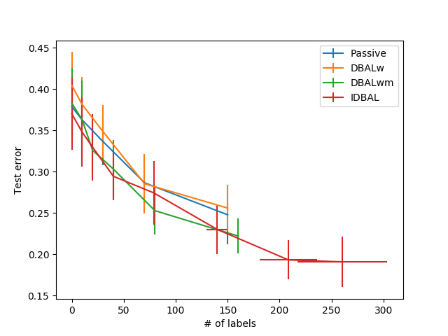
synthetic

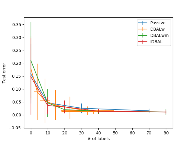
letter

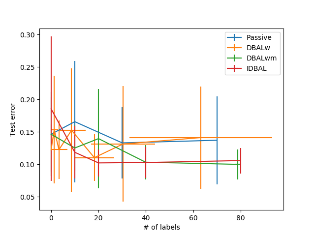
skin

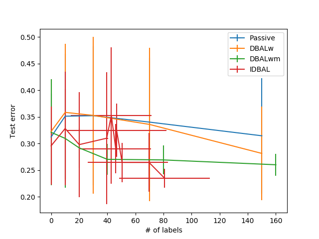
magic

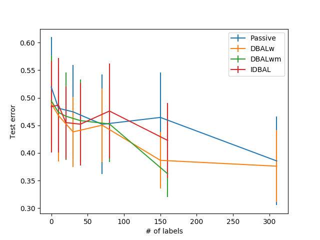
covtype

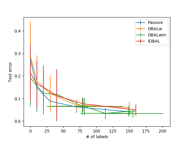
mushrooms

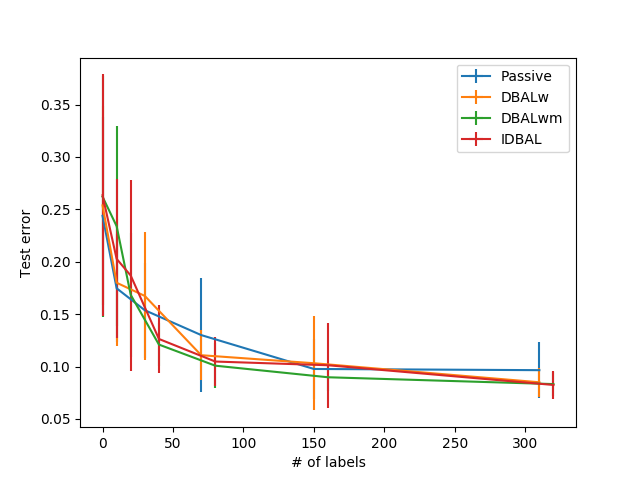
phishing

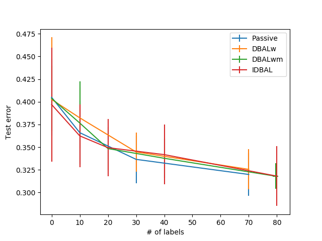
splice

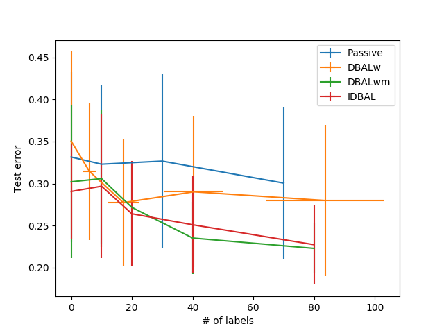
svmguide1

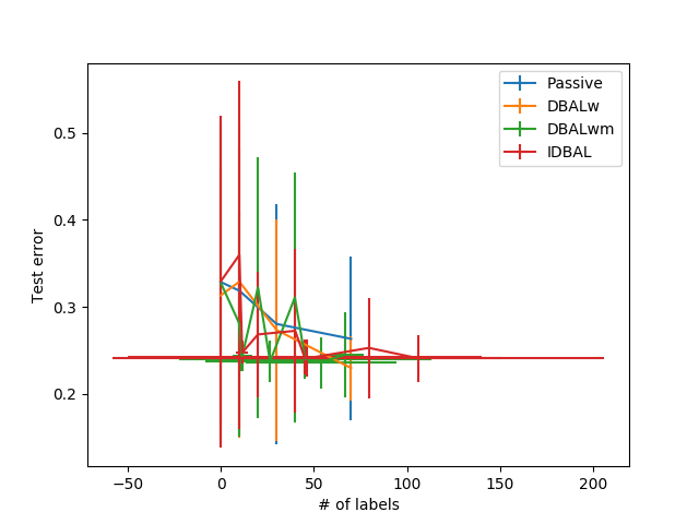
a5a

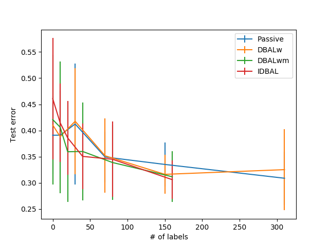
cod-rna

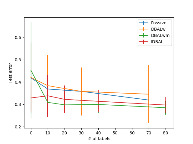
german

Figure 1: Test error vs. number of labels under the Identical policy

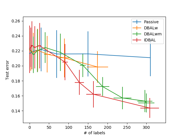
synthetic

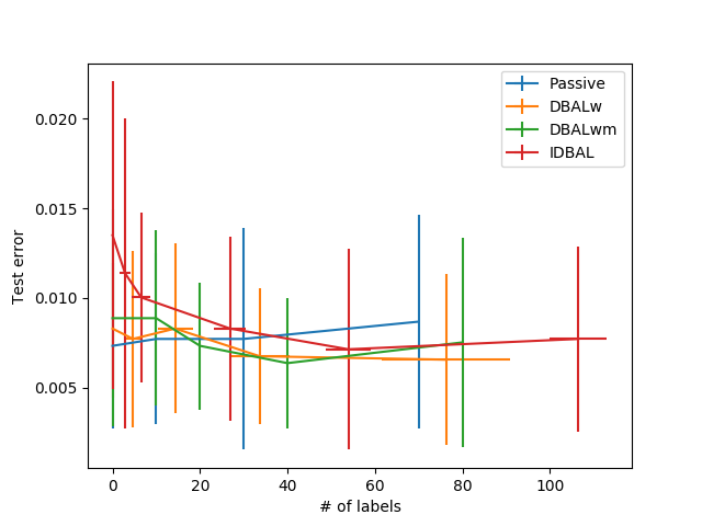
letter

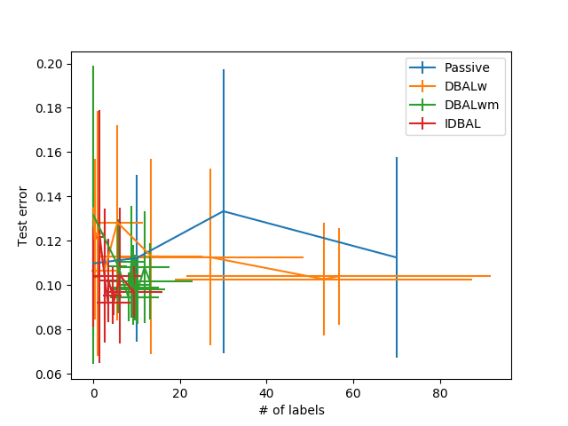
skin

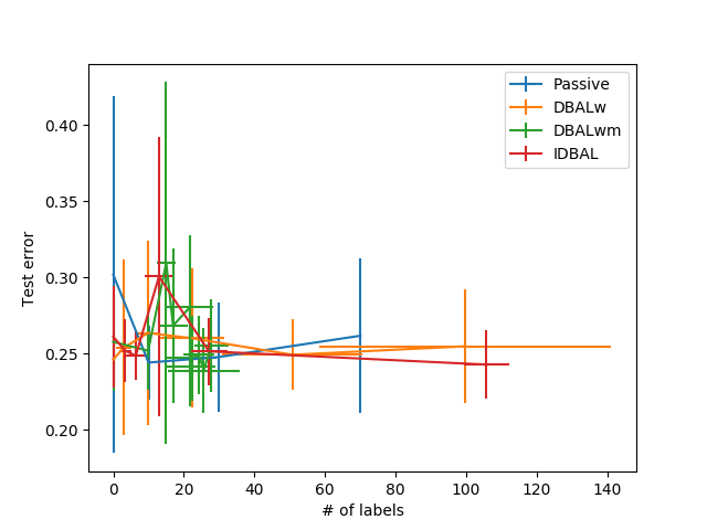
magic

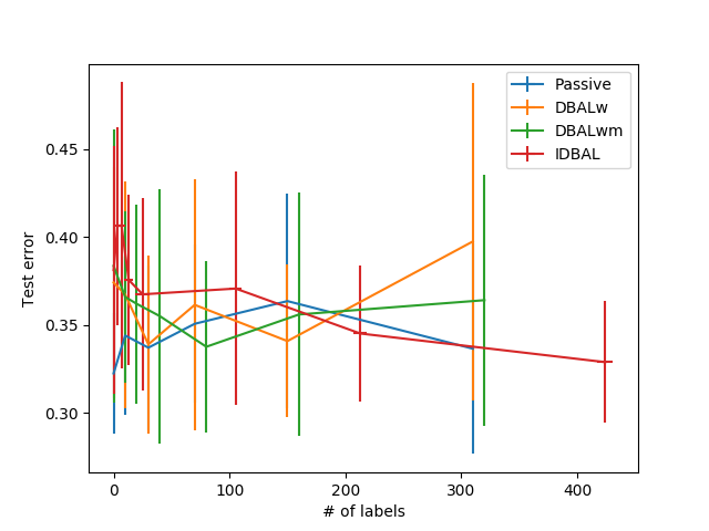
covtype

mushrooms

phishing

splice

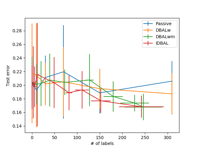
svmguide1

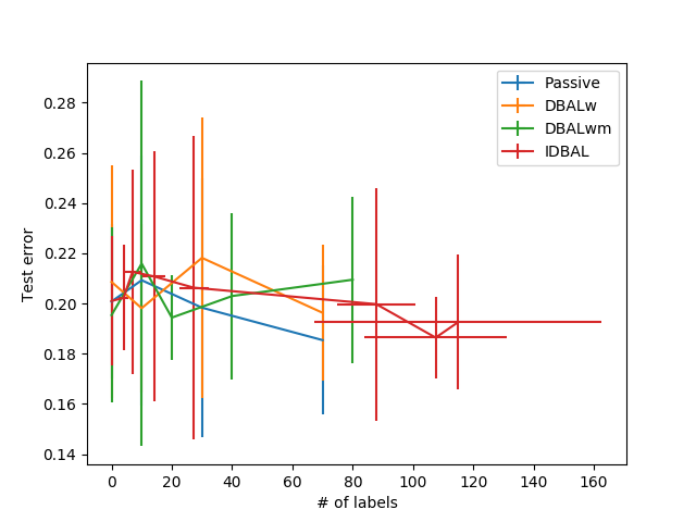
a5a

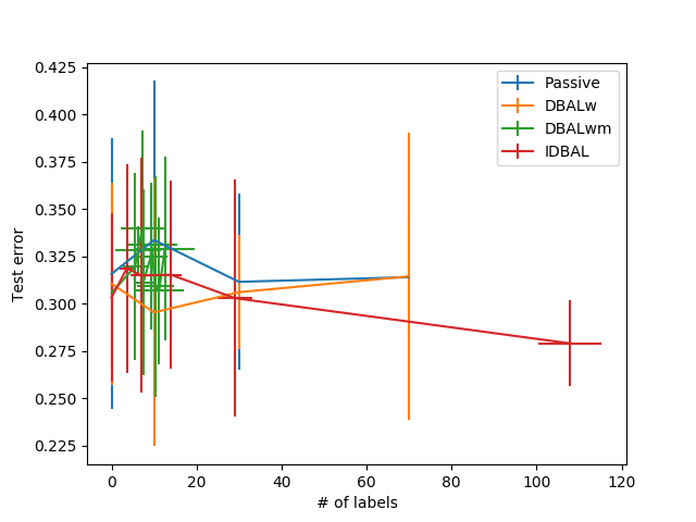
cod-rna

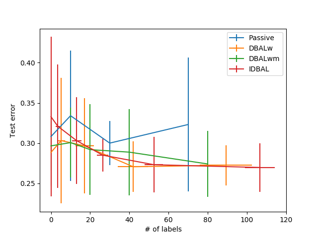
german

Figure 2: Test error vs. number of labels under the Uniform policy

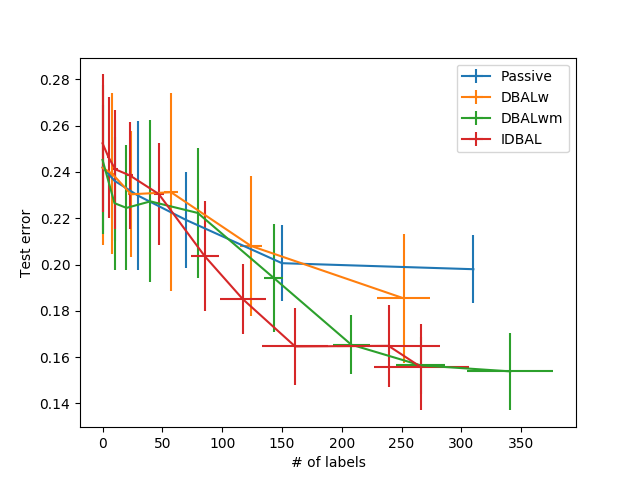
synthetic

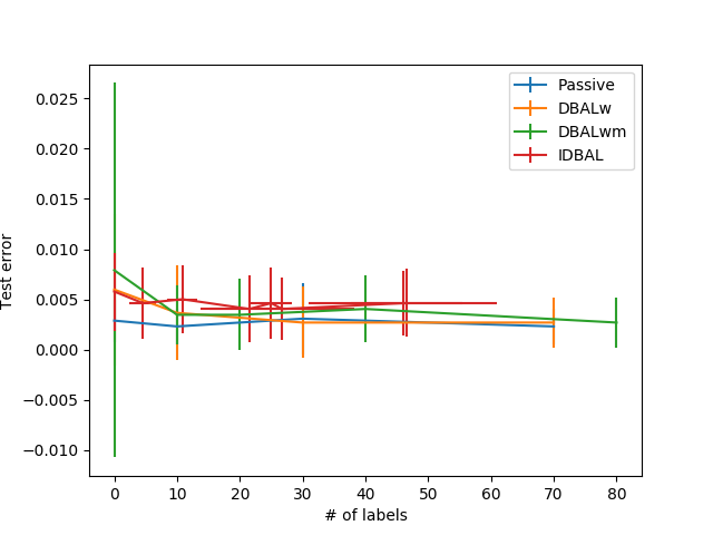
letter

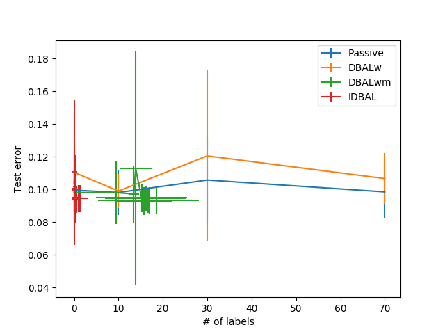
skin

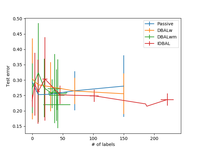
magic

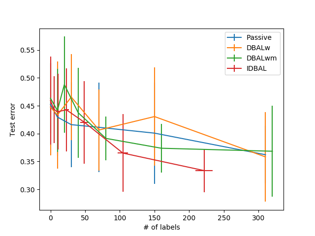
covtype

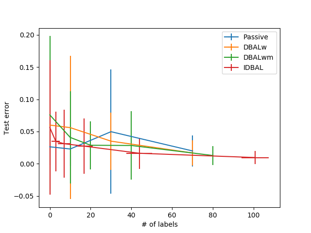
mushrooms

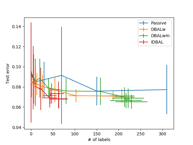
phishing

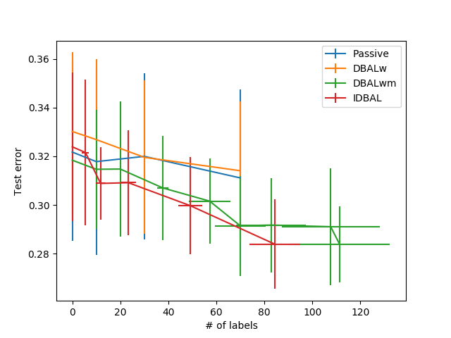
splice

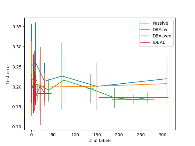
svmguide1

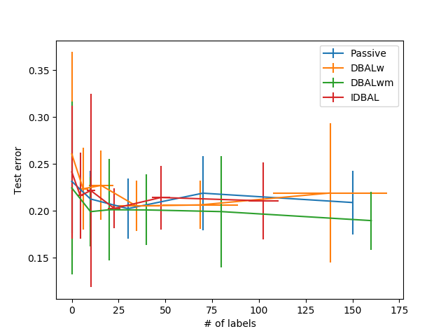
a5a

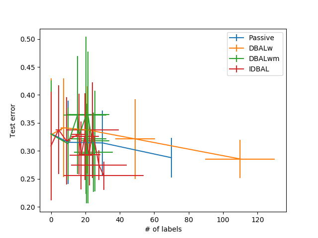
cod-rna

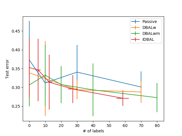
german

Figure 3: Test error vs. number of labels under the Uncertainty policy

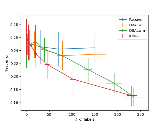
synthetic

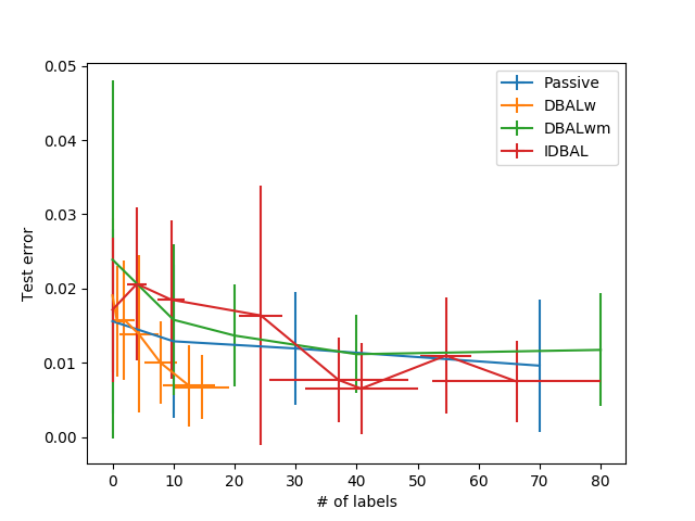
letter

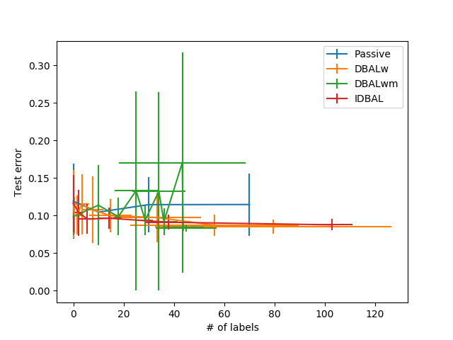
skin

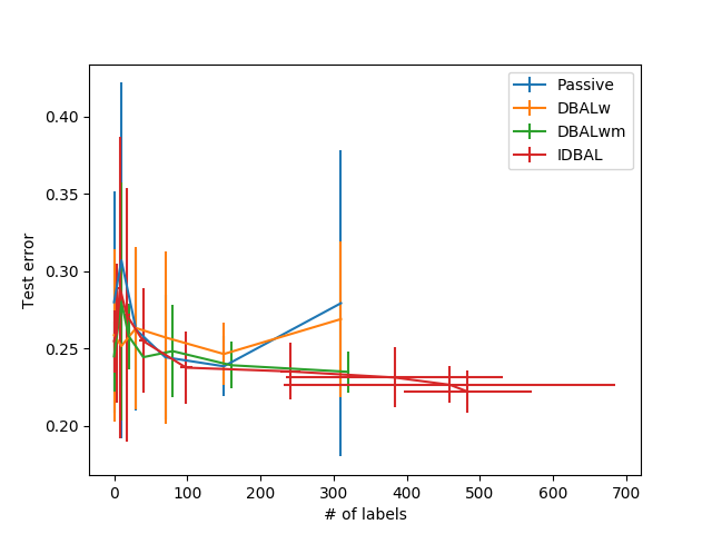
magic

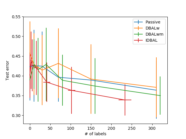
covtype

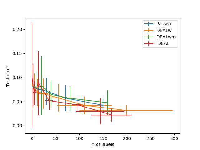
mushrooms

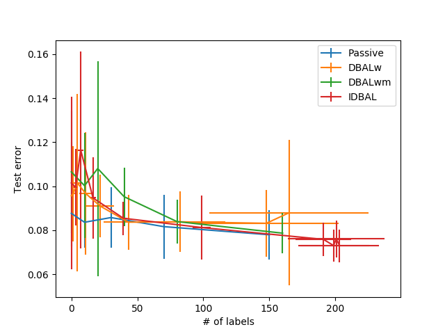
phishing

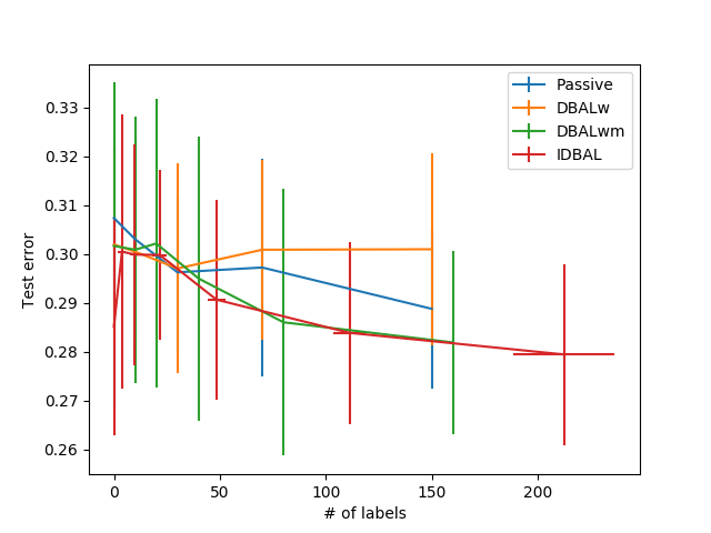
splice

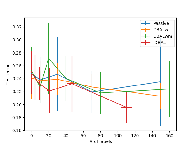
svmguide1

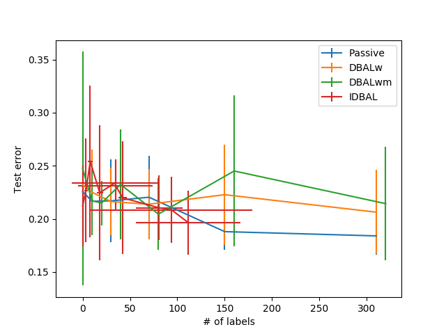
a5a

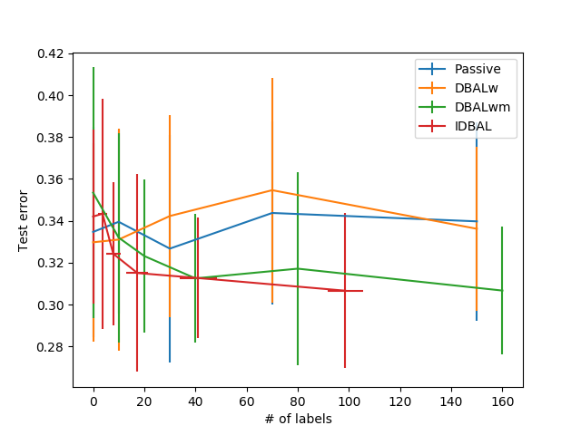
cod-rna

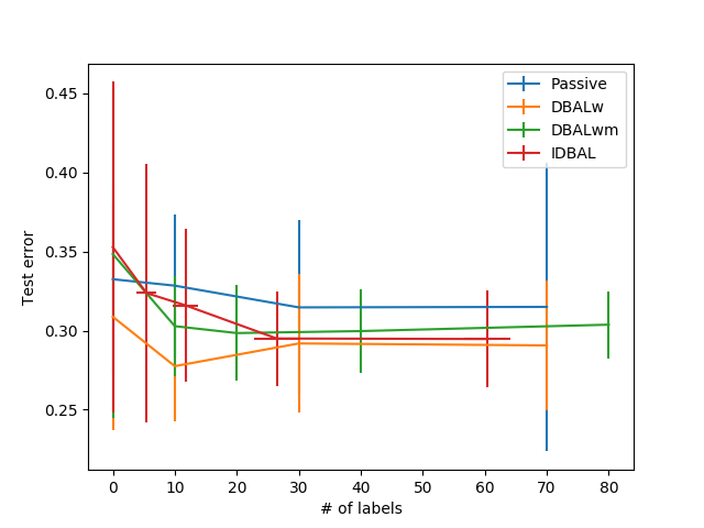
german

Figure 4: Test error vs. number of labels under the Certainty policy

References

• (1) Vowpal Wabbit. https://github.com/JohnLangford/vowpal_wabbit/.
• Agarwal et al. (2014) Agarwal, A., Hsu, D., Kale, S., Langford, J., Li, L., and Schapire, R. Taming the monster: A fast and simple algorithm for contextual bandits. In International Conference on Machine Learning, pp. 1638–1646, 2014.
• Agarwal et al. (2017) Agarwal, A., Basu, S., Schnabel, T., and Joachims, T. Effective evaluation using logged bandit feedback from multiple loggers. arXiv preprint arXiv:1703.06180, 2017.
• Athey & Imbens (2016) Athey, S. and Imbens, G. Recursive partitioning for heterogeneous causal effects. Proceedings of the National Academy of Sciences, 113(27):7353–7360, 2016.
• Balcan et al. (2009) Balcan, M.-F., Beygelzimer, A., and Langford, J. Agnostic active learning. J. Comput. Syst. Sci., 75(1):78–89, 2009.
• Ben-David et al. (2010) Ben-David, S., Blitzer, J., Crammer, K., Kulesza, A., Pereira, F., and Vaughan, J. W. A theory of learning from different domains. Machine learning, 79(1-2):151–175, 2010.
• Beygelzimer et al. (2009) Beygelzimer, A., Dasgupta, S., and Langford, J. Importance weighted active learning. In ICML, 2009.
• Beygelzimer et al. (2010) Beygelzimer, A., Hsu, D., Langford, J., and Zhang, T. Agnostic active learning without constraints. In NIPS, 2010.
• Bottou et al. (2013) Bottou, L., Peters, J., Quiñonero-Candela, J., Charles, D. X., Chickering, D. M., Portugaly, E., Ray, D., Simard, P., and Snelson, E. Counterfactual reasoning and learning systems: The example of computational advertising. The Journal of Machine Learning Research, 14(1):3207–3260, 2013.
• Chang & Lin (2011) Chang, C.-C. and Lin, C.-J. Libsvm: a library for support vector machines. ACM transactions on intelligent systems and technology (TIST), 2(3):27, 2011.
• Cornuet et al. (2012) Cornuet, J., MARIN, J.-M., Mira, A., and Robert, C. P. Adaptive multiple importance sampling. Scandinavian Journal of Statistics, 39(4):798–812, 2012.
• Cortes et al. (2010) Cortes, C., Mansour, Y., and Mohri, M. Learning bounds for importance weighting. In Advances in neural information processing systems, pp. 442–450, 2010.
• Dudík et al. (2011) Dudík, M., Langford, J., and Li, L. Doubly robust policy evaluation and learning. In Proceedings of the 28th International Conference on International Conference on Machine Learning, pp.  1097–1104. Omnipress, 2011.
• Hanneke (2007) Hanneke, S. A bound on the label complexity of agnostic active learning. In ICML, 2007.
• Hanneke & Yang (2015) Hanneke, S. and Yang, L. Minimax analysis of active learning. Journal of Machine Learning Research, 16(12):3487–3602, 2015.
• Hanneke et al. (2014) Hanneke, S. et al. Theory of disagreement-based active learning. Foundations and Trends® in Machine Learning, 7(2-3):131–309, 2014.
• Hofmann et al. (2016) Hofmann, K., Li, L., Radlinski, F., et al. Online evaluation for information retrieval. Foundations and Trends® in Information Retrieval, 10(1):1–117, 2016.
• Hsu (2010) Hsu, D. Algorithms for Active Learning. PhD thesis, UC San Diego, 2010.
• Huang et al. (2015) Huang, T.-K., Agarwal, A., Hsu, D. J., Langford, J., and Schapire, R. E. Efficient and parsimonious agnostic active learning. In Advances in Neural Information Processing Systems, pp. 2755–2763, 2015.
• Jiang & Li (2016) Jiang, N. and Li, L. Doubly robust off-policy value evaluation for reinforcement learning. In Proceedings of the 33rd International Conference on International Conference on Machine Learning-Volume 48, pp.  652–661. JMLR. org, 2016.
• Johansson et al. (2016) Johansson, F., Shalit, U., and Sontag, D. Learning representations for counterfactual inference. In International Conference on Machine Learning, pp. 3020–3029, 2016.
• Kallus (2017) Kallus, N. Recursive partitioning for personalization using observational data. In International Conference on Machine Learning, pp. 1789–1798, 2017.
• Karampatziakis & Langford (2011) Karampatziakis, N. and Langford, J. Online importance weight aware updates. In Proceedings of the Twenty-Seventh Conference on Uncertainty in Artificial Intelligence, pp.  392–399. AUAI Press, 2011.
• Krishnamurthy et al. (2017) Krishnamurthy, A., Agarwal, A., Huang, T.-K., Daumé, III, H., and Langford, J. Active learning for cost-sensitive classification. In Precup, D. and Teh, Y. W. (eds.), Proceedings of the 34th International Conference on Machine Learning, volume 70 of Proceedings of Machine Learning Research, pp.  1915–1924, International Convention Centre, Sydney, Australia, 06–11 Aug 2017. PMLR.
• Li et al. (2010) Li, L., Chu, W., Langford, J., and Schapire, R. E. A contextual-bandit approach to personalized news article recommendation. In Proceedings of the 19th international conference on World wide web, pp.  661–670. ACM, 2010.
• Li et al. (2015) Li, L., Chen, S., Kleban, J., and Gupta, A. Counterfactual estimation and optimization of click metrics in search engines: A case study. In Proceedings of the 24th International Conference on World Wide Web, pp.  929–934. ACM, 2015.
• Lichman (2013) Lichman, M. UCI machine learning repository, 2013. URL http://archive.ics.uci.edu/ml.
• Mandel et al. (2016) Mandel, T., Liu, Y.-E., Brunskill, E., and Popovic, Z. Offline evaluation of online reinforcement learning algorithms. 2016.
• Owen & Zhou (2000) Owen, A. and Zhou, Y. Safe and effective importance sampling. Journal of the American Statistical Association, 95(449):135–143, 2000.
• Rosenbaum & Rubin (1983) Rosenbaum, P. R. and Rubin, D. B. The central role of the propensity score in observational studies for causal effects. Biometrika, 70(1):41–55, 1983.
• Schnabel et al. (2016) Schnabel, T., Swaminathan, A., Singh, A., Chandak, N., and Joachims, T. Recommendations as treatments: Debiasing learning and evaluation. arXiv preprint arXiv:1602.05352, 2016.
• Shalit et al. (2017) Shalit, U., Johansson, F. D., and Sontag, D. Estimating individual treatment effect: generalization bounds and algorithms. In Precup, D. and Teh, Y. W. (eds.), Proceedings of the 34th International Conference on Machine Learning, volume 70 of Proceedings of Machine Learning Research, pp.  3076–3085, International Convention Centre, Sydney, Australia, 06–11 Aug 2017. PMLR.
• Strehl et al. (2010) Strehl, A., Langford, J., Li, L., and Kakade, S. M. Learning from logged implicit exploration data. In Advances in Neural Information Processing Systems, pp. 2217–2225, 2010.
• Sugiyama et al. (2007) Sugiyama, M., Krauledat, M., and MÞller, K.-R. Covariate shift adaptation by importance weighted cross validation. Journal of Machine Learning Research, 8(May):985–1005, 2007.
• Swaminathan & Joachims (2015a) Swaminathan, A. and Joachims, T. Counterfactual risk minimization: Learning from logged bandit feedback. In International Conference on Machine Learning, pp. 814–823, 2015a.
• Swaminathan & Joachims (2015b) Swaminathan, A. and Joachims, T. The self-normalized estimator for counterfactual learning. In Advances in Neural Information Processing Systems, pp. 3231–3239, 2015b.
• Thomas & Brunskill (2016) Thomas, P. and Brunskill, E. Data-efficient off-policy policy evaluation for reinforcement learning. In International Conference on Machine Learning, pp. 2139–2148, 2016.
• Thomas (2015) Thomas, P. S. Safe reinforcement learning. 2015.
• Thomas et al. (2015) Thomas, P. S., Theocharous, G., and Ghavamzadeh, M. High-confidence off-policy evaluation. In AAAI, pp.  3000–3006, 2015.
• Vapnik & Chervonenkis (1971) Vapnik, V. and Chervonenkis, A. Y. On the uniform convergence of relative frequencies of events to their probabilities. Theory of Probability and its Applications, 16(2):264, 1971.
• Veach & Guibas (1995) Veach, E. and Guibas, L. J. Optimally combining sampling techniques for monte carlo rendering. In Proceedings of the 22nd annual conference on Computer graphics and interactive techniques, pp.  419–428. ACM, 1995.
• Wang et al. (2017) Wang, Y.-X., Agarwal, A., and Dudik, M. Optimal and adaptive off-policy evaluation in contextual bandits. In International Conference on Machine Learning, pp. 3589–3597, 2017.
• Zadrozny (2004) Zadrozny, B. Learning and evaluating classifiers under sample selection bias. In Proceedings of the twenty-first international conference on Machine learning, pp.  114. ACM, 2004.
• Zhang & Chaudhuri (2014) Zhang, C. and Chaudhuri, K. Beyond disagreement-based agnostic active learning. In Advances in Neural Information Processing Systems, pp. 442–450, 2014.