KMT-2016-BLG-0212: First KMTNet-Only Discovery of a Substellar Companion

1 Introduction

The Korea Microlensing Telescope Network (KMTNet, Kim et al. 2016) was originally designed to detect and characterize microlensing planets without the need for followup observation.

Gould & Loeb (1992) had originally advocated a two-stage approach to finding microlens planets: in the first stage, a low-cadence, wide-area survey operating from a single site would detect microlensing events in real time and issue alerts to the microlensing community, while in the second stage, a broadly distributed network of narrow-angle telescopes would intensively monitor individual events discovered in the first stage. This strategy was well-matched to the facilities that were available or were considered feasible at that time. Because microlensing events have typical Einstein timescales $t_{\rm E}\sim 20\,$day, they can be reliably discovered in surveys with cadences $\Gamma\sim 1\,{\rm day}^{-1}$. However, because the optical depth to microlensing $\tau\sim 10^{-6}$ is low (even in the densest star fields toward the Galactic bulge), 10–100 square degrees must be monitored to find a large number of events. This is essential for finding planets, because the probability of detecting a planet within a given microlensing event is roughly $q^{1/2}$, where $q$ is the planet/host mass ratio. For relatively common planets $q\sim 10^{-4}$ (Gould et al., 2006, 2010; Sumi et al., 2010; Shvartzvald et al., 2016; Suzuki et al., 2016; Udalski et al., 2018), this probability is therefore 1%. That is, the probability that any given observed star will give rise to a planetary signal is $\sim\tau\sqrt{q}\sim 10^{-8}$, meaning that one must observe several $10^{8}$ stars to have a few events per year with potential planetary signals. On the other hand, to detect a planetary signals requires a cadence $\Gamma$ that is sufficiently high to characterize the brief planetary signal $t_{p}\sim t_{\rm E}\sqrt{q}\rightarrow 5(q/10^{-4})^{1/2}\,{\rm hr}$. That is $\Gamma\sim 1\,{\rm hr}^{-1}$ would be required to characterize “Neptunes” and $\Gamma\sim 4\,{\rm hr}^{-1}$ would be required to detect Earths (Henderson et al., 2014).

The strategy advocated by Gould & Loeb (1992) was successful at finding planets, beginning with OGLE-2005-BLG-071 (Udalski et al., 2005). However, it was fundamentally limited by scarce telescope resources for “stage two” (followup) observations. Indeed, it was only by focusing on high-magnification events, as advocated by Griest & Safizadeh (1998), that the method proved to be as successful as it did.

Second generation surveys by the Microlensing Observations in Astrophysics (MOA, 2006+) and the Optical Gravitational Lensing Experiment (OGLE, 2010+) teams were able to cover very large areas at high cadence $\Gamma=1$–$4\,{\rm hr}^{-1}$, and therefore became capable of both finding microlensing events and characterizing planets without the need for followup observations. For example, Poleski et al. (2014) were able to find and characterize OGLE-2012-BLG-0406Lb based on OGLE data alone. Moreover, by combining the OGLE, MOA, and Wise surveys, Shvartzvald et al. (2016) were able to conduct a survey-only microlensing-planet search with 24-hour coverage, albeit over a limited area.

By combining three 1.6m telescopes with $4\,\deg^{2}$ fields of view on three continents (CTIO, Chile (KMTC), SAAO, South Africa (KMTS), and SSO, Australia (KMTA)), KMTNet is able to monitor about $12\,\deg^{2}$ at $\Gamma=4\,{\rm hr}^{-1}$, $41\,\deg^{2}$ at $\Gamma>1\,{\rm hr}^{-1}$, $85\,\deg^{2}$ at $\Gamma>0.4\,{\rm hr}^{-1}$, and $97\,\deg^{2}$ at $\Gamma>0.2\,{\rm hr}^{-1}$, making it sensitive to, respectively, Earth-mass, Neptune-mass, Saturn-mass, and Jupiter-mass planets over these areas. In the past, this capability has led to the discovery of planets whose perturbations were either inadequately covered (e.g., Han et al. 2017) or not covered at all (e.g., Hwang et al. 2018) by other surveys. However, in these other cases, the event itself was discovered by other surveys, and the planet was found by examining KMTNet data.

Although such combined discoveries are an important contribution, KMTNet also has the potential to independently discover microlensing events, including some with planets and other interesting companions. To date, KMTNet has focused on finding completed events (Kim et al., 2018a) rather than issuing real-time alerts of ongoing events, as for example OGLE has been doing for almost 25 years (Udalski et al., 1994). As discussed by Kim et al. (2018a), this partly reflects the original design of KMTNet as narrowly focused on four fields, for which it had been expected that there would be relatively little role for real-time followup observations. However, even taking account of the revised strategy described above, the decision was still made to focus initially on completed events, simply to catch up with the rapidly accumulating KMTNet light-curve database. While this approach is finding many events that were previously identified by other groups (and so, usually, already examined in KMTNet data), it is also yielding a substantial number of new events that were missed by OGLE and MOA for a variety of reasons, usually non-coverage or coverage that was not adequate to reliably identify the event.

Kim et al. (2018a) developed a new algorithm for finding completed events and applied it to the 2015, i.e., commissioning-year, KMTNet data. In 2016, the observation strategy was substantially changed to that above, covering a roughly six times larger area than the 2015 survey. In addition, the algorithm was upgraded to enable event detection from combined light curves of all three observatories and of overlapping fields. Both changes are likely to lead to a substantial increase in the number of “new events” detected by KMTNet. However, they also both contributed to considerable delay in the public release of the 2016 data relative to the KMTNet goal of releasing within six months of the end of each season (Kim et al., 2018a). Hence, for 2016, we focused initially on an expedited release (Kim et al., 2018b) of KMTNet events in the Kepler-K2 Campaign 9 field (Gould & Horne, 2013; Henderson et al., 2016). This is not a particularly promising domain for new KMTNet events simply because it was heavily covered by all microlensing surveys, including several that were created especially to support Kepler-K2 C9. Nevertheless Kim et al. (2018b) do report a number of such discoveries, including KMT-2016-BLG-0212.

2 Observations and Event Recognition

KMT-2016-BLG-0212 lies at equatorial coordinates (RA, Dec)$=$(17:53:45.42,$-29$:05:12.80), corresponding to Galactic coordinates $(l,b)=(0.79,-1.60)$. It therefore lies in two overlapping KMTNet fields, BLG02 and BLG42. Because these fields strongly overlap the K2 C9 footprint, they were observed at a higher-than-usual combined cadence $\Gamma=6\,{\rm hr}^{-1}$ from KMTS and KMTA beginning April 23 (${\rm HJD}^{\prime}\equiv{\rm HJD}-2450000\sim 7501$). However, because the event had already essentially returned to baseline by this date, this enhanced cadence has almost no practical importance for the present study. Hence, the relevant observations were basically all taken at the standard cadence for BLG02/BLG42 in 2016, $\Gamma=4\,{\rm hr}^{-1}$. As mentioned in Section 1, KMTNet observations are carried out with three identical 1.6m telescopes, each equipped with a $4\,{\rm deg}^{2}$ camera. The cameras are each comprised of four chips (K,M,T,N). The event is located near the chip boundaries so that, by chance, it falls in BLG02T, but in BLG42K, within these two slightly offset fields. The great majority of data were taken in the $I$ band, with about 10% of the KMTC images and 5% of the KMTS images taken in the $V$ band, solely to determine the colors of microlensed sources. For the light curve analysis, the data were reduced using the pySIS software package (Albrow et al., 2009).

KMT-2016-BLG-0212 was originally recognized as “possible microlensing” in the summer of 2017, during a human review of $\sim 5\times 10^{5}$ candidates found by an automatic classifier from among $\sim 3\times 10^{8}$ light curves. The light curves were obtained from difference image analysis (DIA) as implemented using publicly available code from Woźniak (2000). Whenever possible, the DIA input catalog is extracted from the OGLE-III star catalog (Szymański et al., 2011). Otherwise, much shallower, DoPhot (Schechter et al., 1993) catalogs are derived from KMTNet images. KMT-2016-BLG-0212 was identified on the light curve of an $I=19.2$ OGLE-III catalog star. It was judged as “possible” rather than “clear” microlensing because its amplitude is relatively low and the light curve is relatively noisy. Indeed for these reasons, the algorithm found $\Delta\chi^{2}=1521$ (relative to a flat line), which is fairly close to the $\Delta\chi^{2}=1000$ threshold. The anomaly that we will investigate in this paper is not discernible in the DIA light curve, for reasons that we discuss immediately below.

The anomaly was discovered in the course of routine vetting for false positives of all candidates that had been identified in the human review, which was the final step in preparation for the KMTNet-K2 data release (Kim et al., 2018b). This review consisted of viewing side-by-side, an automated pySIS re-reduction of the light curve in the neighborhood of the putative event and a 2016-2017 joint DIA light curve.

The anomaly is quite obvious in the pySIS reductions, which have substantially less noise than the DIA reductions. This is partly because the pySIS “kernel” is better matched to the point spread function (PSF), but mainly because the input catalog star is displaced from the true position of the microlensed source by $0.45^{\prime\prime}$. In particular, the KMTA data that contain the anomaly had exceptionally good seeing (for SSO), as low as FWHM$\sim 1.3^{\prime\prime}$, which (due to the astrometric offset) led to a poor fit, as recorded by the program, and so to photometry that was even noisier than usual. In brief, the re-reductions were essential to the discovery of the anomaly. Note that although the automated pySIS reductions are quite good, the final pySIS reductions were carried out by hand for optimal photometry.

3 Light Curve Analysis

3.1 Heuristic Analysis

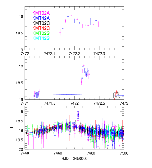
Figure 1: Lightcurve and with single lens (1L1S) model for KMTNet observations of KMT-2016-BLG-0212. The top panel shows the caustic crossing, which is excluded from the fit, while the middle panel shows surrounding regions. The magnitude of the flux variation, $I_{\rm flux-var}\equiv-2.5\log(10^{-0.4I_{\rm peak}}-10^{-0.4I_{\rm base}})\sim 20$ is quite low by the standards of published microlensing events. Here $I_{\rm peak}=18.8$ and $I_{\rm base}=19.2$ are resepectively the peak and baseline of the underlying Paczyński (1986) event.

[h]

Figure 1 shows the KMTNet data with a single-lens single-source (1L1S) model, for which the caustic-region (top panel) data are excluded. The overall characteristics of these data are broadly similar to those of OGLE-2017-BLG-0373 (Skowron et al., 2018): a low-amplitude event with a short, incompletely covered anomaly that appears to be consistent with a planetary caustic. For that event, Skowron et al. (2018) found that there were five different topologies that were roughly consistent with the data, although in the end all but one of these were excluded at $\Delta\chi^{2}\gtrsim 100$. In the present case, the interior of the caustic appears to be more completely covered, but in contrast to OGLE-2017-BLG-0373, neither the caustic entrance nor exit is fully covered. Thus, we proceed cautiously to evaluate all potentially viable topologies. As in the case of OGLE-2017-BLG-0373, we begin with a heuristic analysis of the event (Gould & Loeb, 1992).

The point-lens fit yields Paczyński (1986) parameters $(t_{0},t_{\rm eff},t_{\rm E})=(7465.2,11.2,17.1)\pm(0.2,1.2,2.9)\,$day. Here, $t_{0}$ is the time of lens-source closest approach, $t_{\rm E}$ is the Einstein crossing time, $t_{\rm eff}\equiv u_{0}t_{\rm E}$ is the effective timescale, and $u_{0}$ is the impact parameter (normalized to the angular Einstein radius $\theta_{\rm E}$). From Figure 1, the perturbation is centered at $t_{\rm anom}\simeq{\rm HJD}^{\prime}=7472.3$, implying an offset from the peak of $\delta t=+7.1\,$day. Therefore, if this perturbation is due to a planetary anomaly, then the angle of the source trajectory relative to the binary axis is $\alpha=\tan^{-1}(t_{\rm eff}/\delta t)=57.6^{\circ}\pm 3.0^{\circ}$, and the lens-source separation at the time of the anomaly is $u_{\rm caust}=\sqrt{t_{\rm eff}^{2}+(\delta t)^{2}}/t_{\rm E}=0.78\pm 0.16$. We can then evaluate $s$, the projected separation of the host and companion normalized to $\theta_{\rm E}$, from $|s-s^{-1}|=u_{\rm caust}$, which yields either $s=1.46\pm 0.11$ or $s=0.68\pm 0.05$. Naively, the anomaly in Figure 1 “looks like” a major-image planetary perturbation. Then following the analysis of Skowron et al. (2018) of OGLE-2017-BLG-0373, we note that the above value of $\alpha$ would imply a diagonal caustic crossing and hence a caustic-crossing size best-estimated from the minor diameter $\Delta\eta_{c}=\sqrt{16q/(s^{4}+s^{2})}=1.55q^{1/2}$ (Han, 2006). The caustic coverage is incomplete, but appears to be slightly more than half over when the KMTA data end. We therefore estimate $t_{\rm caust}=0.3$ days, from which we derive $q=((t_{\rm caust}/t_{\rm E})/1.55)^{2}=1.3\times 10^{-4}$.

3.2 Grid Search

The exercise in Section 3.1 shows, based on cursory inspection of the light curve, that there is likely to be a $q\sim 10^{-4}$ major-image solution, but it does not show that this solution is either unique or best. Indeed, Skowron et al. (2018) showed that for the qualitatively similar case OGLE-2017-BLG-0373, there were four additional topologies that yielded viable fits to the data.

We therefore undertake a systematic grid search to find all such topologies. We first hold $(s,q)$ fixed at $100^{2}$ pairs of values [$(-1\leq\log s\leq 1)\times(-5\leq\log q\leq 0)$], while seeding the other parameters at $(t_{0},u_{0},t_{\rm E})$ as derived above, $\rho=10^{-3}$, and $\alpha$ at 10 equally spaced values around a circle. We employ Markov Chain Monte Carlo (MCMC) $\chi^{2}$ minimization to find the best grid-point model. We then seed new MCMCs with local minima on the $(s,q)$ plane derived from this grid search. We find that there are six other viable topologies (in addition to the one heuristically derived in Section 3.1). Moreover, very similar to OGLE-2017-BLG-0373, we find two different geometries (“wide 2” and “wide 3”) within the topology identified in Section 3.1). We further divide “wide 2” into “wide 2a” and “wide 2b” because this broad minimum in the $\chi^{2}$ surface weakly separates into two sub-minima. Figure 2 shows the source trajectories for these nine different solutions.

Figure 2: Source trajectory and caustic geometries for nine solutions, representing seven different topologies.

[h]

3.3 Elimination of Some Topologies

Table 1: Lensing parameters of close models

Parameters	close 1	close 2	close 3	close 4
$\chi^{2}$	9150.54	9216.07	9173.89	9316.97
$\rm{dof}$	9147	9147	9147	9147
$t_{0}$ $(\rm{HJD}^{\prime})$	7463.052$\pm$0.249	7465.385$\pm$0.193	7465.209$\pm$0.195	7463.171$\pm$0.260
$u_{0}$	0.328$\pm$0.013	0.591$\pm$0.037	0.515$\pm$0.029	0.418$\pm$0.020
$t_{\rm E}$ $(\rm{days})$	26.616$\pm$0.880	17.860$\pm$0.763	19.896$\pm$0.781	19.906$\pm$0.718
$s$	0.829$\pm$0.007	0.709$\pm$0.013	0.735$\pm$0.011	0.791$\pm$0.005
$q$ $(10^{-4})$	368$\pm$61	8.889$\pm$1.395	3.054$\pm$0.475	2467$\pm$205
$\alpha$ $(\rm{rad})$	3.131$\pm$0.060	4.044$\pm$0.017	4.168$\pm$0.017	5.086$\pm$0.034
$\rho$ $(10^{-3})$	1.192$\pm$0.207	1.173$\pm$0.203	1.371$\pm$0.218	–

Table 2: Lensing parameters of wide models

Parameters	wide 1	wide 2a	wide 2b	wide 3	wide 4
$\chi^{2}$	9183.84	9157.18	9159.21	9158.52	9214.34
$\rm{dof}$	9147	9147	9147	9147	9147
$t_{0}$ $(\rm{HJD}^{\prime})$	7466.971$\pm$0.217	7465.316$\pm$0.192	7465.250$\pm$0.197	7465.276$\pm$0.189	7466.843$\pm$0.204
$u_{0}$	0.224$\pm$0.010	0.615$\pm$0.020	0.617$\pm$0.022	0.619$\pm$0.018	0.160$\pm$0.014
$t_{\rm E}$ $(\rm{days})$	36.288$\pm$1.210	17.764$\pm$0.476	17.801$\pm$0.478	17.584$\pm$0.440	38.853$\pm$2.457
$s$	1.070$\pm$0.005	1.427$\pm$0.014	1.430$\pm$0.015	1.434$\pm$0.012	1.685$\pm$0.060
$q$ $(10^{-4})$	359$\pm$39	0.490$\pm$0.079	0.828$\pm$0.153	0.484$\pm$0.110	1153$\pm$216
$\alpha$ $(\rm{rad})$	0.013$\pm$0.022	1.004$\pm$0.0145	1.001$\pm$0.0153	1.005$\pm$0.014	0.867$\pm$0.022
$\rho$ $(10^{-3})$	0.791$\pm$0.139	1.378$\pm$0.278	1.666$\pm$0.283	1.874$\pm$0.430	–

Table 3: Physical properties

Quantity	close 1	wide 2a	wide 2b	wide 3
Is - Iclump	4.645$\pm$0.080	3.558$\pm$0.077	3.551$\pm$0.077	3.550$\pm$0.077
(V-I)s - (V-I)clump	-0.29$\pm$0.12	-0.23$\pm$0.11	-0.23$\pm$0.11	-0.24$\pm$0.11
$\theta_{\rm E}$ [mas]	0.42$\pm$0.10	0.64$\pm$0.22	0.53$\pm$0.14	0.47$\pm$0.15
$\mu$ [mas]	8.1$\pm$1.9	13.2$\pm$4.5	10.9$\pm$2.9	9.8$\pm$3.1
$M$ [$M_{\odot}$]	0.49${}_{-0.26}^{+0.37}$	0.38${}_{-0.22}^{+0.38}$	0.41${}_{-0.23}^{+0.38}$	0.373${}_{-0.21}^{+0.37}$
$m_{\rm p}$	19${}_{-12}^{+20}\,M_{\rm Jup}$	6.2${}_{-4.0}^{+8.2}\,M_{\oplus}$	11.3${}_{-7.2}^{+14.4}\,M_{\oplus}$	6.0${}_{-4.0}^{+8.6}\,M_{\oplus}$
$D_{\rm L}$ [kpc]	6.3${}_{-1.5}^{+1.1}$	6.1${}_{-1.7}^{+1.3}$	5.9${}_{-1.6}^{+1.3}$	6.2${}_{-1.6}^{+1.2}$
$a_{\perp}$ [AU]	2.2${}_{-0.5}^{+0.5}$	5.5${}_{-1.9}^{+2.0}$	4.5${}_{-1.2}^{+1.2}$	4.2${}_{-1.4}^{+1.4}$

These nine solutions are given in Tables LABEL:tab:close and LABEL:tab:wide. Three of these solutions (“close 2”, “close 4” and “wide 4”) have $\chi^{2}$ values that are substantially higher than the others. Figure 3, which shows the light-curve fits over the anomaly, implies that a major reason for this is a very poor fit of the latter two (“close 4” and “wide 4”) to the anomaly. We consider that these are eliminated. The remaining solutions fit the anomaly reasonably well.

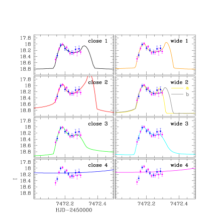
Figure 3: Zoom of fits for nine different model geometries of KMT-2016-BLG-0212 over the anomaly. Solutions “close 4” and “wide 4” have poor fits and are excluded.

[h]

Figure 4 shows the overall form of the nine models, and Figure 5 shows the residuals of the data for each model.

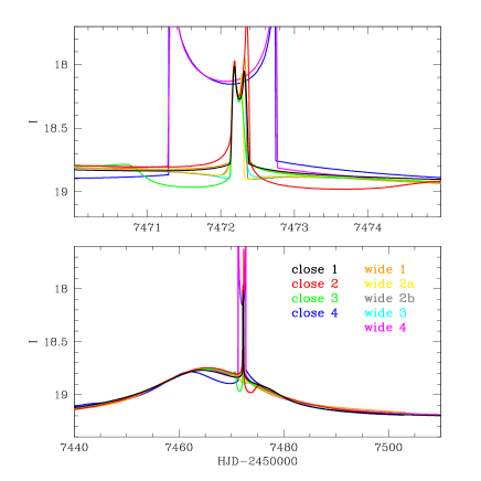
Figure 4: Comparison of nine models (without data) that are broadly compatible with the data. The upper panel is a zoom of the region near the caustic.

[h]

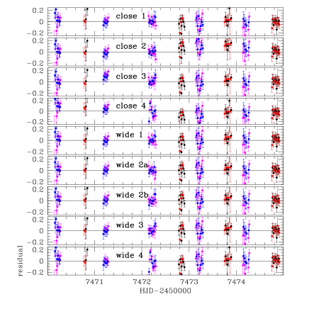
Figure 5: Residuals of the data relative to the nine models shown in Figure 4. The quite poor match of model “close 2” during the 1.5 days centered on HJD${}^{\prime}\sim 7473.5$ explains the high $\chi^{2}$ of this model. The origin of the relatively high $\chi^{2}$ of “close 3” model is the systematic deviation of the model in KMTA data near HJD${}^{\prime}\sim 7471.2$. The mismatch of models “close 4” and “wide 4” are noticeable here but are more apparent in Figure 3.

[h] Figure 5 shows that the high $\chi^{2}$ of model “close 2” is due to systematically high residuals during four consecutive episodes of KMTC, KMTA, KMTC, KMTA observations beginning HJD${}^{\prime}\sim 7472.8$, which is explained by the long post-caustic “dip” of this model in Figure 4. It also shows that the relatively high $\chi^{2}$ of model “close 3” is primarily due to systematic residuals near HJD${}^{\prime}\sim 7471.2$. Comparing to Figure 4, we see that this is due to the strong “dip” in this model just prior to the caustic crossing. Finally, we note that although “wide 1” has even higher $\chi^{2}$ than “close 3”, there are no strong residuals within the range displayed in Figure 5. The main problem for this model comes from its long “relative trough” (compared to “close 1”) after the caustic exit, $7473\lesssim{\rm HJD^{\prime}}\lesssim 7480$. See Figure 4. This issue also impacts “close 3”, albeit at a lower level.

3.4 Summary of Surviving Models

This series of rejections leaves models “close 1”, “wide 2a”, “wide 2b”, and “wide 3”, which have mass ratios, $q=3.7\times 10^{-2}$, $q=4.9\times 10^{-5}$, $q=8.3\times 10^{-5}$, and $q=4.8\times 10^{-5}$, respectively. The first solution (“Class I”) which, depending on the host mass, could be a brown dwarf or a high-mass planet, is preferred over the other three by $\Delta\chi^{2}\geq 6.8$. Hence, it is favored, but not decisively. The other three solutions have $q\lesssim 10^{-4}$.

This second class of solutions (“Class II”) are part of the same topology, namely the one that was naively investigated in Section 3.1. Comparison to Table LABEL:tab:wide shows that the simple reasoning in that section predicted the parameters of these solutions reasonably well.

This event is similar to the case of OGLE-2017-BLG-0373 (Skowron et al., 2018). Also similar to that case, there are multiple geometries within this topology that are qualitatively similar but can differ significantly in the mass ratio $q$. However, what is fundamentally different about the present case is that one of the alternate topologies (which were not anticipated by the naive reasoning of Section 3.1) is competitive with (and indeed slightly preferred over) the naive solution.

We note, however, that the two classes of solutions differ by a factor 2.5 in their source flux $f_{s}$, i.e., by $\sim 1\,$mag in source magnitude (see Section 4.1). As we discuss in Section 5, this will ultimately enable one to distinguish between these two classes of solutions.

4 Physical Parameters

As just discussed, there are two classes of solutions with very different topologies and very different planet-host mass ratios $q$. The first class has only one local minimum (“close 1”), with $q=0.037$. The second class has three local minima (“wide 2a”, “wide 2b”, “wide 3”), with $q$ ranging from $4.8\times 10^{-5}$ to $8.3\times 10^{-5}$. For the second class, all the remaining parameters are essentially the same with the exception of $\rho$, and even the three values of $\rho$ are basically consistent with one another within their rather large errors. See Table LABEL:tab:wide. Therefore, there are likewise two classes of physical parameters for the host, with a factor $\sim 1.8$ range in planet-host mass ratio within the second class.

4.1 Color-Magnitude Diagram

The first step toward estimating the physical parameters is to locate the source star on a color-magnitude diagram. The source color should be independent of the model and should, in fact, be measurable without reference to any model, i.e., by regression. However, this proves not to be the case for KMT-2016-BLG-0212. In 2016, KMTNet took $V$-band data from KMTC and KMTS. Since the source lies in two overlapping fields (BLG02 and BLG42), the source color can in principle be determined independently from four different data sets. However, the faintness of the source in $V$-band and the low-amplitude of the event together render regression-based $(V-I)$ color estimates unstable. Hence, we must measure both the source color and magnitude from each of the four $V/I$ data sets within the framework of specific models. We perform a special set of pyDIA reductions of the data (i.e., different from the pySIS reductions from the main light-curve analysis) because these simultaneously yield field-star photometry on the same system as the light curve. Unfortunately, the $V$-band light curve from KMTS02 is not usable. Hence, for each of the four surviving models, we have three independent measures of the source color $(V-I)_{s}$ and four independent measures of the source magnitude $I_{s}$. In each case, we find the offset of these quantities from the clump. In Table LABEL:tab:quant we present the means and standard errors of the mean for these three (color) or four (magnitude) measures. Figure 6 shows the pyDIA color-magnitude calibrated to OGLE-III (Szymański et al., 2011) including the position of the red clump and the locations of the source for the two classes of solution.

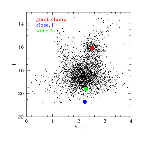
Figure 6: Color-magnitude diagram (CMD) from pyDIA reductions of KMTNet data, calibrated to OGLE-III (Szymański et al., 2011). The positions of the clump and of the source for two of the solutions (“close 1” and “wide 2a”) are shown. The source positions for the other two “Class II” solutions (“wide 2b” and “wide 3”) are nearly identical to “wide 2a”.

[h]

We see from these results that from the standpoint of the source color and magnitude, there are essentially two classes of solutions, close BD-class companion (Class I) and wide sub-Neptune-class companion (Class II). We adopt the dereddened clump color and magnitude $[(V-I),I]_{\rm clump,0}=(1.06,14.44)$ from Bensby et al. (2013) and Nataf et al. (2013), convert from $V/I$ to $V/K$ using the color-color relations of Bessell & Brett (1988), and then apply the color/surface-brightness relations of Kervella et al. (2004) to obtain

$$\theta_{*}=0.51\pm 0.09\,{\mu\rm as}\quad({\rm I}),\quad\theta_{*}=0.89\pm 0.19\,{\mu\rm as}\quad({\rm II})$$ (1)

Then using the values (and errors) of $\rho$ and $t_{\rm E}$ from Tables LABEL:tab:close and LABEL:tab:wide, one obtains the Einstein radius $\theta_{\rm E}=\theta_{*}/\rho$ and proper motion $\mu=\theta_{\rm E}/t_{\rm E}$, as given in Table LABEL:tab:quant. We note that these two physical quantities are unusually poorly constrained. This is partly due to the large errors in $\theta_{*}$, which is caused by the relatively poor measurement of $(V-I)_{s}$, and partly due to the large errors in $\rho$, which is caused by the incomplete coverage of the caustic entrance.

We can nevertheless make a Bayesian estimate of the physical parameters, i.e., the lens mass $M$, the companion mass $m_{p}$, the lens distance $D_{L}$ and the companion-host projected separation $a_{\perp}$. To do so, we draw lens and source kinematics randomly from a Han & Gould (1995) Galactic model and draw host masses randomly from a Chabrier (2003) mass function. We then weight these by how well they match the measured $t_{\rm E}$ and $\mu$ and also by the microlensing rate $\propto\mu\theta_{\rm E}$. The distributions of the host-mass and system distance for the two classes of solutions are illustrated in Figures 7 and 8. These distributions peak near $M\sim 0.5\,M_{\odot}$ and $D_{L}\sim 6\,{\rm kpc}$, but are quite broad.

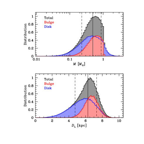
Figure 7: Bayesian estimates, based on the Han & Gould (1995) Galactic model for the host mass and system distance of KMT-2016-BLG-0212 for the “close 1” (BD-class) solution. The distributions are quite broad.

[h]

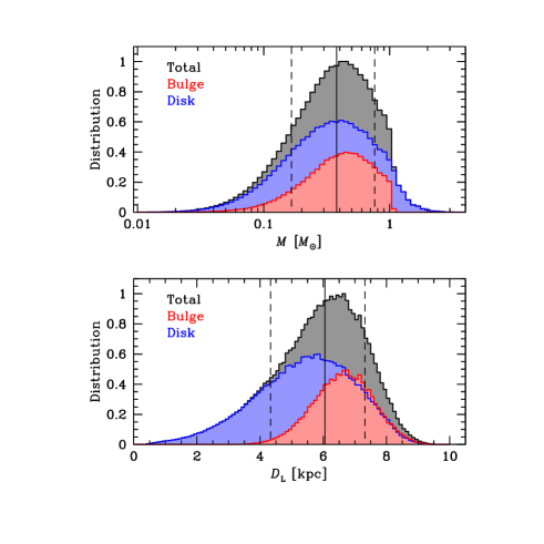
Figure 8: Bayesian estimates, based on the Han & Gould (1995) Galactic model, for the host mass and system distance of KMT-2016-BLG-0212 for the “wide 2a” (sub-Neptune-class) solution. The distributions are qualitatively similar to those of the “close 1” solution (Figure 7). They are also extremely similar to the distributions for the “wide 2b” and “wide 3” solutions, for which reason these latter are not shown.

[h]

We find estimated parameter ranges as described in Table LABEL:tab:quant. As expected, the companion of “close 1” (“BD”) solution peaks at a value typical of low-mass BDs, although it overlaps the “traditional planetary” range $m_{p}<13\,M_{\rm jup}$. The companions for the three “Class II” (“sub-Neptune”) solutions peak in the Super-Earth regime but are also quite broad. In Section 5, we discuss how these two classes of solutions can be distinguished by future high-resolution imaging of the source. While this is the main outstanding issue in the interpretation of this event, we note that by also resolving the lens, such observations would simultaneously allow much more precise determination of the host mass than is returned from the Bayesian analysis presented in this section. For the case that such imaging favors the “Class I” solution, the mass of the companion will be determined quite precisely. However, for the “Class II” solutions, the companion mass will still be uncertain by a factor $\sim 2$ because the values of $q$ differ by this amount between solution “wide 2b” on the one hand, and the solutions “wide 2a” and “wide 3” on the other. See Table LABEL:tab:wide.

5 Future Resolution

The $q=0.037$ (“brown dwarf”) solution is favored over the $q\lesssim 10^{-4}$ (“sub-Neptune”) solutions by $\Delta\chi^{2}=6.64$, which formally corresponds to $p=\exp(-\Delta\chi^{2}/2)=3.6\%$. This would not be enough to decisively rule out the latter even if the statistics of the data were strictly Gaussian. Moreover, systematics at this level are quite common in microlensing. However, because these two classes of solutions differ in their source flux by $\Delta I_{s}\simeq 1\,$mag, it will be straightforward to distinguish between them with high-resolution imaging, i.e., either adaptive optics (AO) imaging from the ground or with a high-resolution space telescope, e.g., the Hubble Space Telescope (HST). This can certainly be done once the source and lens separate, but there is a good chance that an observation taken immediately could distinguish between the two classes of solutions. In particular, if the flux at the position of the source is significantly below the level expected for the brighter (“sub-Neptune”) solution, then this would confirm the fainter (“brown dwarf”) solution. However, if the measured flux is consistent with or brighter than the brighter solution, then the excess may be due to the lens (or possibly a companion to the source or the lens). In this case, additional observations would be required once the source and lens have separated.

One potential difficulty with ground-based AO observations is that these are essentially always done in the near-IR. Since we do not have a good measurement of the source color, we cannot directly predict the source flux in IR bands. However, if the AO observations were conducted in two IR band passes (e.g., $J$ and $K$), then the $I$-band source flux could be determined by making use of an $IJK$ color-color diagram. For reference, we note that based on OGLE-III data (Szymański et al., 2011) within $75^{\prime\prime}$ of the lens, the clump lies at $[(V-I),I]_{\rm clump}=(2.52,16.06)$.