The Progenitor Age and Mass of the Black Hole Formation Candidate N6946-BH1

Abstract

The failed supernova N6946-BH1 likely formed a black hole (BH); we age-date the surrounding population and infer an age and initial mass for the progenitor of this BH formation candidate. First, we use archival Hubble Space Telescope imaging to extract broadband photometry of the resolved stellar populations surrounding this event. Using this photometry, we fit stellar evolution models to the color-magnitude diagrams to measure the recent star formation history (SFH). Modeling the photometry requires an accurate distance; therefore, we measure the tip of the red giant branch (TRGB) and infer a distance modulus of $29.47\pm 0.079$ to NGC 6946, or a metric distance of $7.83\pm 0.29$ Mpc. To estimate the stellar population’s age, we convert the SFH and uncertainties into a probabilistic distribution for the progenitor’s age. The region in the immediate vicinity of N6946-BH1 exhibits the youngest and most vigorous star formation for several hundred pc. This suggests that the progenitor is not a runaway star. From these measurements, we infer an age for the BH progenitor of $10.6^{+14.5}_{-5.9}$ Myr. Assuming that the progenitor evolved effectively as a single star, this corresponds to an initial mass of $17.9^{+29.9}_{-7.6}$ $M_{\odot}$. Previous spectral energy distribution (SED) modeling of the progenitor suggests a mass of $\sim$27 $M_{\odot}$. Formally, the SED-derived mass falls within our narrowest 68% confidence interval; however, $91\%$ of the probability distribtuion function we measure lies below that mass, putting some tension between the age and the direct-imaging results.

1 Introduction

In general, stellar evolution theory predicts that stars with masses above about 8 $M_{\odot}$ undergo core collapse (Woosley et al., 2002). Even though most of these likely explode, it is not entirely clear which actually do. Therefore, observations are crucial for identifying which stars do or do not explode.

Although the details vary, theories suggest that black hole (BH) formation should be primarily seen for more massive progenitors. At the low-mass end, both theory (Woosley et al., 2002; Ugliano et al., 2012; Sukhbold et al., 2016; Bruenn et al., 2016; Burrows et al., 2018) and observations (Jennings et al., 2014; Smartt, 2015; Davies & Beasor, 2018) suggest that there is a minimum mass for core collapse and most progenitors above this minimum mass explode and do not form BHs (Woosley et al., 2002, 7-8 $M_{\odot}$). CCSN simulations suggest that stars near the minimum mass explode quite easily (Radice et al., 2017), even in one-dimensional simulations. Slightly higher mass stars, above an initial mass (the zero-age main-sequence (MS) mass, $M_{\rm ZAMS}$) of $\sim$9 $M_{\odot}$, require the extra boost given by multidimensional simulations (Murphy & Burrows, 2008; Melson et al., 2015; Roberts et al., 2016; Bruenn et al., 2016; Mabanta & Murphy, 2018). Therefore, according to single-star stellar evolution theory and bolstered by the large number of observations of low-mass progenitors of supernovae (SNe) and SN remnants (Smartt, 2009; Davies & Beasor, 2018; Maund, 2017; Jennings et al., 2012, 2014; Díaz-Rodríguez et al., 2018) , it is unlikely that BH formation will be seen in the lowest-mass stars.

In contrast, CCSN simulations find that the most massive stars have difficulty exploding (Ugliano et al., 2012; Sukhbold et al., 2016). Instead, a fair fraction of these most massive stars fail to explode and form BHs. These investigations also suggest that the mapping between $M_{\rm ZAMS}$ and final outcome may not be entirely correlated or monotonic (Sukhbold et al., 2017). There are islands of failed SNe as a function of mass, and these islands tend to become larger and more frequent toward the highest masses. These analyses present a very clear prediction: that the distribution of progenitors that fail to explode should be heavily skewed toward the most massive progenitors. Testing this prediction requires measuring a large number of progenitor masses for CCSNe and/or BH formation events.

While significant progress has been made in building up statistics of progenitor masses for successful CCSNe (Smartt, 2009; Jennings et al., 2012, 2014; Williams et al., 2014a, 2018), measurements of failed explosions have only just begun. Kochanek et al. (2008) proposed to identify “failed” explosions by monitoring nearby galaxies for massive stars that disappear without a SN and instead form a BH. From this survey, Gerke et al. (2015) identified several candidates for further monitoring. Of these, Adams et al. (2017) identified the vanishing star, N6946-BH1, as the most promising BH formation candidate. In addition, Reynolds et al. (2015) performed a similar but more limited survey using Hubble archival imaging of 15 galaxies. They reported a failed SN candidate, which will require further monitoring. In this paper, we provide an independent measure of the age and $M_{\rm ZAMS}$ for N6946-BH1 by age-dating the surrounding stellar population using techniques developed in Gogarten et al. (2009); Murphy et al. (2011); Jennings et al. (2012, 2014); Williams et al. (2014a).

Measuring a mass for N6946-BH1 is of the highest importance for core-collapse theory. By modeling the color and magnitude of the progenitor, Adams et al. (2017) estimated the progenitor’s initial mass to be $M_{\rm ZAMS}\sim 25M_{\odot}$. This technique of interpreting precursor imaging is based on using stellar evolutionary tracks to model the observed magnitude and color of the progenitor. If the observations include most of the bolometric luminosity, then estimating the progenitor mass is straightforward. For the most part, the luminosity of a post-MS star is determined by the mass of the helium core and hydrogen-burning shell (Woosley et al., 2002). In turn, the helium core size is set by the zero-age MS mass. Hence, with broad spectral coverage, one can directly infer the progenitor mass. However, more frequently, one only has observations in just a few spectral bands, making modeling the luminosity extremely sensitive to mass-loss history and dust formation in the last uncertain stages of stellar evolution. As a result, the mass inferred for the progenitor depends sensitively on uncertain bolometric corrections (see, for example, the Davies & Beasor (2018) reanalysis of Smartt (2009) data on red supergiant progenitors).

Given the importance of measuring the mass of N6946-BH1, we take an independent approach to constraining the progenitor mass: we age-date the stellar population, and from this age, we infer the mass of the star that would reach the end of its lifetime at that age. This technique has the advantage that the age is sensitive to many phases of stellar evolution and features in the color-magnitude diagram (CMD), not just the final uncertain stage of stellar evolution. For example, the tip of the MS provides an upper limit on the age, and the presence of helium burners helps to constrain specific ages. The tip of the MS is dependent upon the well-understood physics of the MS, and helium burners are an early, more certain post-MS stage. This technique has now been used and validated extensively (Gogarten et al., 2009; Murphy et al., 2011; Jennings et al., 2012, 2014; Williams et al., 2014a).

In this manuscript, we age-date the stellar population in the vicinity of N6946-BH1. We age-date the stellar population for two reasons. One, it provides an independent check on the direct technique that relies on modeling the uncertain physics of late-stage evolution. Two, even if there is an inconsistency between the two techniques, it may further illuminate the evolutionary scenario – for example, by pointing toward binary evolution models. Assuming single-star evolution for the progenitor, we then infer the progenitor mass and compare it to the mass derived directly from the spectral energy distribution (SED) of the progenitor.

The presentation of this manuscript is as follows. In the method section ( § 2), we describe the parameters of N6946-BH1, including those previously determined. We also describe the method for our age-dating technique. In particular, we formalize how to transform the star formation history (SFH) and uncertainties into an age distribution for the progenitor. In the results section (§ 3) we determine the age, infer a progenitor mass, and consider how various biases (such as kicks) may affect the age and mass. Finally, we conclude that the age is $10.6^{+14.5}_{-5.9}$ Myr and the progenitor mass is $17.9^{+29.9}_{-7.6}$ $M_{\odot}$.

2 Method

To derive the progenitor mass of N6946-BH1, we employ the following procedure. We first derive F438W, F606W, and F814W photometry for Hubble Space Telescope (HST) observations covering the location of N6946-BH1 (§ 2.1). We then characterize the completeness, biases, and uncertainties in the photometry by successfully inserting and recovering artificial stars. We use the resulting model of photometric effects to derive the SFH (§ 2.3) by modeling the F606W-F814W CMD for stars surrounding N6946-BH1 using the fitting program MATCH (Dolphin, 2002a, 2012, 2013). To derive a full probability distribution for the stellar population that produced N6946-BH1, we consider a variety of assumptions for choice of analysis area (§ 2.1), distance (§ 2.2), and dust (§ 2.3). We then translate this age distribution into a distribution for the progenitor mass (§ 2.4).

2.1 Photometry

We used pipeline-calibrated HST Wide Field Camera 3 (WFC3) UVIS images from several general observing campaigns. See Table 1 for the proposal IDs, PI, filters, and total exposure times. Figure 1 shows an image for the region surrounding N6946-BH1. The location of the progenitor for N6946-BH1 was at the center of the red circle, R.A. 20:35:27.56 and decl. +60:08:08.29. The GO-13392 images were taken on 2014 February 21, the GO-14266 images were observed on 2015 October 8, and the GO-14786 images were taken on 2016 October 26, which is 5-7 yr after the observations in which the N6946-BH1 had disappeared (2009).

We derived photometry from the images using a modified version of the PHAT pipeline, which is built around DOLPHOT (Dolphin, 2002b; Williams et al., 2014b). We selected stars with signal-to-noise ratio ${\rm SNR}>4$, sharpness squared $<0.15$, and crowding $<1.3$. We combined the photometry from all epochs of imaging; the resulting data reach a depth of 27.64, 28.23, and 26.74 in F438W, F606W, and F814W, respectively. These correspond to the brightness of a solar-metallicity MS star with mass 12, 9, and 15 $M_{\odot}$ respectively (Marigo et al., 2017). To convert these magnitude depths into MS mass, we assume a distance to NGC 6946 of $7.83\pm 0.29$ Mpc (see the derivation of the distance in § 2.2) and total foreground extinction of $A(V)=0.94$ (Schlafly & Finkbeiner, 2011; Adams et al., 2017).

Table 1: Data sets for inferring the SFH in the vicinity of the vanisher, N6946-BH1

Prop ID	PI	Filter	Exposure Time (s)
13392	B. Sugerman	F438W	2768
13392	B. Sugerman	F606W	1744
13392	B. Sugerman	F814W	1744
14266	C. Kochanek	F606W	1233
14266	C. Kochanek	F814W	1233
14786	B. Williams	F438W	2670
14786	B. Williams	F606W	2800

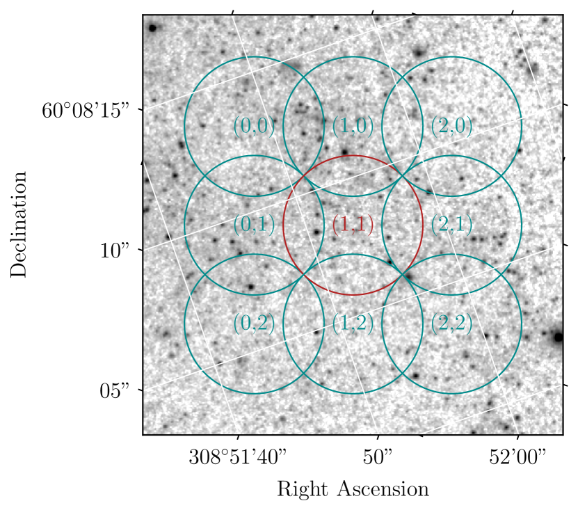
Figure 1: HST F606W drizzled image showing the region surrounding the vanishing star and BH candidate, N6946-BH1. We identify all of the stars in this region, model the color-magnitude diagram, and infer the age of the stellar population surrounding the vanisher. The central red circle is a region surrounding the vanisher with a radius of 100 pc (the distance to NGC 6496 is $7.83\pm 0.29$ Mpc). It is possible that the vanisher was born in another nearby region and received a kick to its current location. Later, we model this uncertainty by inferring the star formation region for the eight surrounding regions (blue circles), each with a radius of 100 pc.

Gerke et al. (2015) measured the photometry for the progenitor of N6946-BH1 from HST archival images. The resulting magnitudes are $23.09\pm 0.01$ in F606W and $20.77\pm 0.01$ in F814W.

Figure 1 also shows regions for which we characterize the stellar populations. The red circle is centered on the vanisher. We adopt a radius of 100 pc for these regions. Early experiments on the size of the region (Gogarten et al., 2009) suggested that $\sim$50 pc is big enough to include a significant number of MS stars for age-dating but not too big to include too many stars from neighboring populations. However, that exploration was for one region of one galaxy, and the optimum size will likely differ depending upon the local stellar density. For now, we adopt 100 pc radii and leave a more thorough analysis on the dependence of size for future work. In addition to the region centered on the vanisher, we also infer the age of eight nearby 100 pc radius regions (blue circles), which allows us to consider scenarios in which the vanisher was ejected from a neighboring star-forming region. For a characteristic ejected velocity of $\sim$10 km s^-1 and a lifetime of $\sim$10 Myr, the vanisher could have traveled 100 pc before undergoing core collapse.

In Figure 2, we plot the F814W versus F606W-F814W (top panel) and F606W versus F438W-F606W (bottom panel) CMDs for the central region colocated with the vanisher. The star in the top plot represents the photometry of N6946-BH1 before it vanished in the optical bands (Gerke et al., 2015). Before N6946-BH1 vanished, it was the brightest star in the F814W filter in this region. In fact, it is the brightest star within 300 pc. Later, we find the SFH both with and without the progenitor; it made no real difference in the resulting SFH. For reference, we plot isochrones for six ages (7, 10, 14, 19, 25, and 50 Myr) assuming solar metallicity and a foreground reddening of $A(V)=0.94$ and $R(V)=3.1$ (Marigo et al., 2017).

We infer the SFH for both F438W versus F438W-F606W and F606W versus F606W-F814W CMDs independently, but we only report the more accurate SFH for F606W vs. F606W-F814W. In principle, one may use MATCH to infer an SFH based upon all three bands. However, MATCH is not able to calculate the uncertainty in the SFH based upon three bands. It calculates the uncertainty for two or four bands. We find that the SFH is a little more accurate when using the F606W and F814W bands. Furthermore, the progenitor is extremely red and only has upper limits for F438W (Adams et al., 2017). To give a broader sense of the CMD, we report both CMDs, but for inferring SFHs and ages, we primarily report ages using the F606W and F814W CMD.

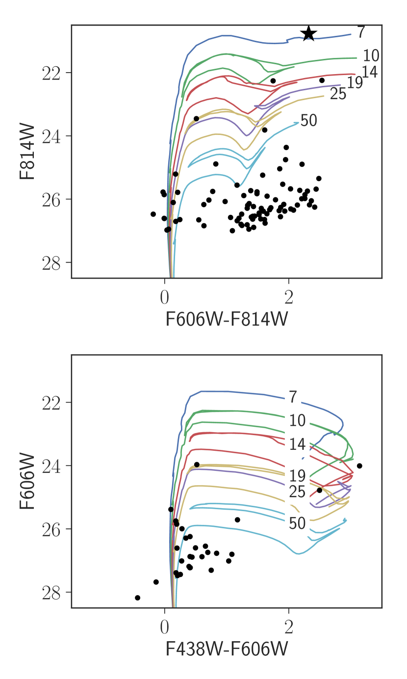
Figure 2: The CMDs for a region within 100 pc of the vanisher. The bottom panel shows F606W vs. F438W-F606W, and the top panel shows F814W vs. F606W-F814W. The star in the top panel shows the photometry for N6946-BH1 before it vanished (Gerke et al., 2015). For comparison, both plots also show model isochrones for 7, 10, 14, 19, 25, and 50 Myr. The distance is $7.83\pm 0.29$ Mpc with an $A(V)$ of 0.94. We use MATCH to infer the SFH from the F606W-F814W CMD.

2.2 Distance to NGC 6946

When inferring the SFH, one must convert model luminosities into model fluxes; this requires an accurate distance to NGC 6946. NGC 6946 has had roughly 10 observed SNe in the last 50 yr, so deriving an accurate distance to this one galaxy will greatly improve the statistics of many local SNe. Here we describe our method to calculate the distance to NGC 6946 using the tip of the red giant branch (TRGB).

There are 32 distance estimates in the NASA/IPAC Extragalactic Database (NED) with a mean of 5.5 Mpc and a standard deviation of 1.5 Mpc. A variety of techniques were used to determine these distances; they include the brightest blue stars, Tully-Fischer, TRGB, and the expanding photosphere for SN Type II methods. The reported uncertainties on most of the distance moduli are of order 0.1. Gerke et al. (2015) and Adams et al. (2017) used a distance of 5.9 Mpc derived from the brightest blue stars method (Karachentsev et al., 2000). However, we note that Karachentsev et al. (2000) actually reported a distance of 6.8 Mpc for NGC 6946. The confusion in distance from Karachentsev et al. (2000) is understandable. The text of that manuscript only refers to the average distance to the NGC 6946 group (5.9 Mpc), but Table 4 of Karachentsev et al. (2000) explicitly gives the distance to NGC 6946 as 6.8 Mpc. More recently, Tikhonov (2014) used the expanding photosphere method and inferred a distance of $6.72\pm 0.15$ Mpc. In any case, these distance measures are fairly uncertain compared to a well-calibrated TRGB distance estimate.

McQuinn et al. (2016) described a precise method for determining the distance from the TRGB. Our first step is to use HST images to calculate accurate photometry for a large number of stars in NGC 6946. The images were taken in the F606W and F814W bands by program HST-GO-14786 (PI: B. Williams). They contain 5470 s of exposure in F606W and 5538 s of exposure in F814W. They reach 27.5 in F814W and 28.6 in F606W. They were observed on 2016-11-02 pointed at R.A. = 308.8530225, decl. = 60.040649634. We derived F606W and F814W photometry from the images using a modified version of the PHAT pipeline, which is built around DOLPHOT (Dolphin, 2002b; Williams et al., 2014b). The TRGB location was measured using a Bayesian maximum-likelihood technique described in McQuinn et al. (2016), which is based on Makarov et al. (2006).

The measured TRGB magnitude is $26.004\pm 0.035$ at a color of ${\rm F606W}-{\rm F814W}=1.71$. The fit is clean; in particular, there are no secondary peaks that might indicate issues. With a total foreground extinction of $A(V)=0.94$ (Schlafly & Finkbeiner, 2011; Adams et al., 2017), the corresponding reddenings are $A({\rm F606W})=0.88$ and $A({\rm F814W})=0.57$. Therefore, the reddened-corrected TRGB is 25.44 with a color of 1.40. Rizzi et al. (2007) provided a calibration for the absolute magnitude for the TRGB: $M({\rm ACS}\,{\rm F814W})=-4.06+0.20[({\rm F606W}-{\rm F814W})-1.23]$. Given the reddening-corrected color, the F814W absolute magnitude is $M({\rm ACS}\,{\rm F814W})=-4.03.$ Sources of uncertainty in the Rizzi et al. (2007) calibration and its underlying horizontal-branch (HB) calibration (Carretta et al., 2000) add 0.05 mag of uncertainty, while an adopted 10% uncertainty in the foreground extinction adds another 0.05 mag of uncertainty (Schlafly & Finkbeiner, 2011). Combined with the measurement uncertainty, we calculate a distance modulus of $m-M=29.47\pm 0.079$. The corresponding metric distance is $7.83\pm 0.29$ Mpc.

This new distance for NGC 6946 suggests that the vanisher was intrinsically 1.3 times more luminous than assumed in Adams et al. (2017). According to the Marigo et al. (2017) models, the larger distance would shift their mass estimate from $\sim$25 $M_{\odot}$ to $\sim$27 $M_{\odot}$. As a rough measure of systematics in the stellar evolution models, Adams et al. (2017) also estimated the mass using rotating models. Their SED-derived mass from the rotating models was $\sim$22 $M_{\odot}$. With the new distance, this would shift to $\sim$24 $M_{\odot}$.

2.3 Star Formation History

We derive SFHs from the F606W-F814W CMD using the program MATCH (Dolphin, 2002a, 2012, 2013), which generates model CMDs that include the effects of observational errors (as characterizing the artificial star tests), foreground and internal dust extinction, and distance and then adjusts the SFHs to maximize the likelihood of the observed CMD. We run MATCH using logarithmically spaced age bins, $\Delta\log_{10}(t\text{yr}^{-1})=0.05$, and the left edge of the minimum age bin is $\log_{10}(t\text{yr}^{-1})=6.6$). Using the TRGB distance, we fix the distance to be 7.83 Mpc.

We assume an extinction law with $R(V)=A(V)/E(B-V)=3.1$ (Cardelli et al., 1989; O’Donnell, 1994) and use the same galactic foreground reddening as Adams et al. (2017) of $E(B-V)=0.303$ (Schlafly & Finkbeiner, 2011) to fix the foreground extinction in MATCH to be $A(V)=0.94$. However, we allow MATCH to fit for a distribution of internal extinctions; the default model in MATCH uses a top-hat distribution of extinction, with width $dA_{V}$. This is designed to approximate the behavior of young stars enshrouded in a layer of patchy dust. We infer $dA_{V}$ for each region in Figure 1. Starting from the top left, the values for $dA_{V}$ are 0.00, 0.19, and 0.00 (top row); 0.70, 0.39, and 0.00 (middle row); and 0.05, 0.17, and 0.00 (bottom row). Taking the internal extinction as a tracer of the presence of molecular gas, one might expect the youngest population to be in the region containing the vanisher and the region to its left in Figure 1.

2.4 Deriving the Age PDF from the SFH and Uncertainties

The SFH provides the stellar mass formed as a function of age. To estimate the age probability distribution function (PDF), we assume that the probability is proportional to the mass of stars formed. If one knows the exact SFH, then the age PDF would simply be proportional to the best-fit SFH. However, MATCH provides a hybrid Markov chain Monte Carlo (MCMC) algorithm, which returns a distribution of SFHs given the photometric data of the surrounding stars. Therefore, one must derive the age distribution given the distribution of accepted SFHs.

The goal is to derive the marginalized age distribution $P(\tau)$, given the distribution of SFHs ($\{S_{j}(\tau)\}$) that MATCH returns; $j$ indexes each MCMC sample. When converting an SFH to a PDF, one must choose a maximum age for the normalization. A reasonable choice for this maximum age is the maximum age for core collapse, $T_{\rm max}$. Given these assumptions and dependencies, the joint probability for observing a burst of star formation is $P(\tau,S,T_{\rm max})$. Marginalizing this distribution gives the age PDF

$$P(\tau)=\int P(\tau,S,T_{\rm max})\,dS\,dT_{\rm max}\,.$$ (1)

To derive the joint probability distribution, we use the conditional probability theorem, which states that

$$P(\tau,S,T_{\rm max})=P(\tau|S,T_{\rm max})P(S)P(T_{\rm max})\,.$$ (2)

Here $P(\tau|S,T_{\rm max})$ is the likelihood for $\tau$ given the SFH, $S$, and maximum age in converting the SFH into a PDF, $T_{\rm max}$:

$$P(\tau|S,T_{\rm max})=\frac{S(\tau)}{M_{\star}(T_{\rm max})}\,,$$ (3)

where $M_{\star}=\int_{0}^{T_{\rm max}}S(\tau)\,d\tau$ is the total stellar mass formed in the last $T_{\rm max}$ years. Here $P(S)$ represents the distribution of SFHs from MATCH hybrid MCMC runs, and $P(T_{\rm max})$ represents a prior on $T_{\rm max}$. Díaz-Rodríguez et al. (2018) recently found the maximum age for core collapse to be $50.3^{+2.5}_{-0.5}$ Myr, and one could use this distribution as the prior. However, this distribution is preliminary in that the Díaz-Rodríguez et al. (2018) analysis does not include the uncertainties in the SFH in the conversion from SFH to PDF. The work of this section will provide the foundation for a more thorough analysis. Therefore, for the purposes of this manuscript, we will employ the same prior that was used in previous studies (Gogarten et al., 2009; Murphy et al., 2011; Williams et al., 2014a); we will only consider ages below $\widetilde{T}_{\rm max}$ in the conversion from an SFH to a PDF. Hence, the prior for $T_{\rm max}$ is a delta function at $\widetilde{T}_{\rm max}$:

$$P(T_{\rm max})=\delta(T_{\rm max}-\widetilde{T}_{\rm max})\,,$$ (4)

where $\widetilde{T}_{\rm max}=50$ Myr. This prior simplifies the marginalization in eq. (1) to

$$P(\tau)=\int P(\tau|S,\widetilde{T}_{\rm max})P(S)\,dS\,.$$ (5)

MATCH returns discreet samples of SFHs with star formation rates (SFRs) at discreet ages; hence, the age PDF will be discreet. In general, samples returned by MCMC algorithms are designed so that the density of the samples is proportional to the probability density function. Therefore, the probability of each SFH sample is

$$P(S)=\frac{1}{N}\,,$$ (6)

where $N$ is the number of samples. The discreet marginalized PDF for the age then becomes

$$P(\tau_{i})=\frac{1}{N}\sum_{j=1}^{N}\frac{S_{j}(\tau_{i})}{M_{j}(\widetilde{T}_{\rm max})}\,.$$ (7)

The index $i$ specifies the age bin, $j$ specifies the MCMC sample, and $M_{j}(\widetilde{T}_{\rm max})$ is the total stellar mass formed in the last $\widetilde{T}_{\rm max}$ yr. If the total mass formed is the same for each sample, then the discreet marginalized PDF is equal to the average SFH divided by the total stellar mass formed in the last $\widetilde{T}_{\rm max}$ years.

2.5 Reporting the Confidence Interval

In this manuscript, we report the most likely age and the narrowest 68% confidence interval (CI). Alternatively, one might report the 68% CI bounded by the 16th and 84th percentiles. However, this often-used technique is prone to several biases when applied to real data. If the PDF has exceptionally large wings, as real data often do, then the 16th and 84th percentiles tend to be centered around the median, not the mode. The age PDF in Figure 3 has a relatively narrow mode but very large wings. Therefore, if we simply report the 16th and 84th percentiles, then the CI will be strongly biased to the middle of the age range that we consider. Effectively, this CI will be centered around $\widetilde{T}_{\rm max}/2$, making the CI strongly dependent upon the maximum age chosen for normalization. Reporting the narrowest 68% CI mitigates these problems. The narrowest 68% CI is less sensitive to the large wings in the PDF, is much less dependent on $\widetilde{T}_{\rm max}$, and naturally centers on the mode of the distribution.

3 Results and Discussion

Figure 3 shows the SFH and the age distribution, $P(\tau)$, based upon the F606W-F814W CMD for the central 100 pc radius region in the vicinity of N6946-BH1. The top panel shows the best-fit SFH (blue bars) and uncertainties (gray regions). The uncertainties represent the distribution of MCMC sample SFHs. The top panel also shows the best-fit cumulative distribution function (CDF) within the last 50 Myr (black line). The gray region represents the 68% CI on the cumulative distribution. Along the top horizontal axis, this figure shows the $M_{\rm ZAMS}$ that dies at the age of the lower horizontal axis. For this age-to-mass mapping, we use the results of PARSEC v1.2S isochrones (Marigo et al., 2017). There are two bursts of star formation within the last 50 Myr; the highest SFR is found in the most recent one, at $\sim$10 Myr. This age corresponds to a progenitor mass of $\sim$18 $M_{\odot}$. The next oldest burst, at $\sim$23 Myr, would correspond to a much lower mass ($\sim$10 $M_{\odot}$).

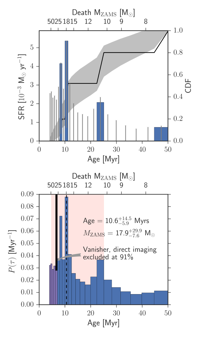
Figure 3: Age distribution for the 100 pc region surrounding the vanisher, N6946-BH1. The top panel shows the SFH. The blue bars show the best-fit SFH from MATCH, and the gray uncertainties represent the distribution of SFHs from MCMC runs. The top panel also shows the CDF in the last 50 Myr (black line with 68% CI in gray). The bottom panel shows the marginalized age distribution, the most likely age (vertical dashed line), and the narrowest 68% CI (rose band). We find the most likely age to be $10.6^{+14.5}_{-5.9}$ Myr, and the corresponding birth mass is $M_{\rm ZAMS}=17.9^{+29.9}_{-7.6}$ $M_{\odot}$. The vertical black bar shows the SED-derived mass (Adams et al., 2017). The SED-derived mass is different than the best-fit age-derived mass, but the results are formally consistent.

To test the sensitivity of the SFH to the presence of the vanisher, we derived the SFH for two scenarios. In one, we included the photometric properties of the vanisher. In the second, we omitted the vanisher. The resulting SFHs and uncertainties were nearly identical. These results suggest that the SFH is not sensitive to the presence or absence of the progenitor.

The bottom panel of Figure 3 shows the marginalized age distribution for the stellar population, $P(\tau)$ (blue bars). Assuming that the progenitor evolved as a single star and was born with the surrounding population, then the most likely age for the progenitor is $10.6^{+14.5}_{-5.9}$ Myr. This corresponds to an $M_{\rm ZAMS}=17.9^{+29.9}_{-7.6}$. The dashed line shows the most likely age and mass, and the rose-colored region shows the narrowest 68% CI. The vertical black bar shows the SED-derived mass estimate for the vanisher (Adams et al., 2017). Formally, the SED-derived mass falls within the narrowest 68% CI; however, $91\%$ of the PDF we measure lies below that mass, putting some tension between the age and the direct-imaging results.

The narrowest 68% CI for the age lies between 4.7 and 25.1 Myr. In contrast, the 16% and 84% percentiles are 8.4 and 34.1 Myr. While the SED-derived mass and age lie within the narrowest 68% CI, it lies outside the 68% range based upon the percentiles. The narrowest 68% CI is a more reliable estimator of the distribution’s width near the mode because the large tails heavily bias the calculation of the percentiles toward the middle of the distribution.

Figure 4 compares the model CMD (Hess diagram) with the observed F606W versus F606W-F814W CMD. The background blue-scale image represents the Hess diagram for the best-fit model in the top panel of Figure 3. The shade of blue represents the number of expected stars per Hess bin, where each Hess bin is 0.1 mag in height and 0.05 mag in the width (color). The black circles are the observed stars within 100 pc of the vanisher, and the star shows the color and magnitude of the vanisher. In general, the model accurately represents the density of stars along the MS and the helium burners. The low-luminosity red giants in the lower right contribute to ages in the star formation that are older than 50 Myr. The upper MS and the few bright yellow and red supergiants constrain the young ages.

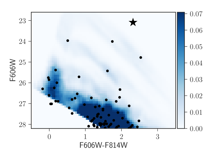
Figure 4: Comparison between the Hess diagram (modeled CMD) and the observed CMD. The points show the observed CMD and the F606W magnitude vs. the color, F606W-F814W. The color map represents the model. The blue shading presents the expected number of stars per Hess bin; each Hess bin has a width in color of 0.05 and a height in magnitude of 0.1. This modeled CMD represents the best-fit SFH in the top panel of Figure 3. The model accurately represents the observed MS, including the MS turnoff, the red helium burners (the four or five red and yellow supergiants), and the swarm of red giants (lower right) associated with older ages. The star represents the magnitude and color of the vanisher.

It is possible that the progenitor is not coeval with the surrounding stellar population, which could impact the certainty of the age and progenitor mass. For example, stellar dispersion and kicks are two mechanisms that may cause the progenitor to no longer be located with its coeval birth population. The birth velocity dispersions of massive stars is of order 5 or 10 km s^-1 (Oh et al., 2015; Aghakhanloo et al., 2017), reflecting the gravitational potential of the molecular clouds from which they form. After 10 Myr, such a velocity dispersion would mean that the star has moved 50 – 100 pc. Fortunately, if one star disperses, many stars might disperse as well, and in this case, the progenitor’s birth companions would still be within the central 100 pc. Even if one considers more significant kicks, it is likely that many of the coeval birth population received kicks, and again, the progenitor’s birth companions would be found in the same region (Eldridge et al., 2011). Still, it is possible that the progenitor was in a binary companion and received a large kick, propelling it 100 pc or more before collapse.

To assess the uncertainties associated with this scenario, we calculate the SFH and ages for the eight regions adjacent to the central one. Figures 5 and 6 show the CMDs for the surrounding regions, along with the same isochrones as in Figure 2, for reference. Of all the CMDs, the central region has the highest number of bright MS stars, which is a clear indication that the central region has a best-fit SFH with the youngest and most prominent burst of star formation. Also, note that the progenitor (the star in Figure 6) is the brightest star in all regions, which makes it the brightest star within 100 pc. One has to go 300 pc before finding a star at least as bright.

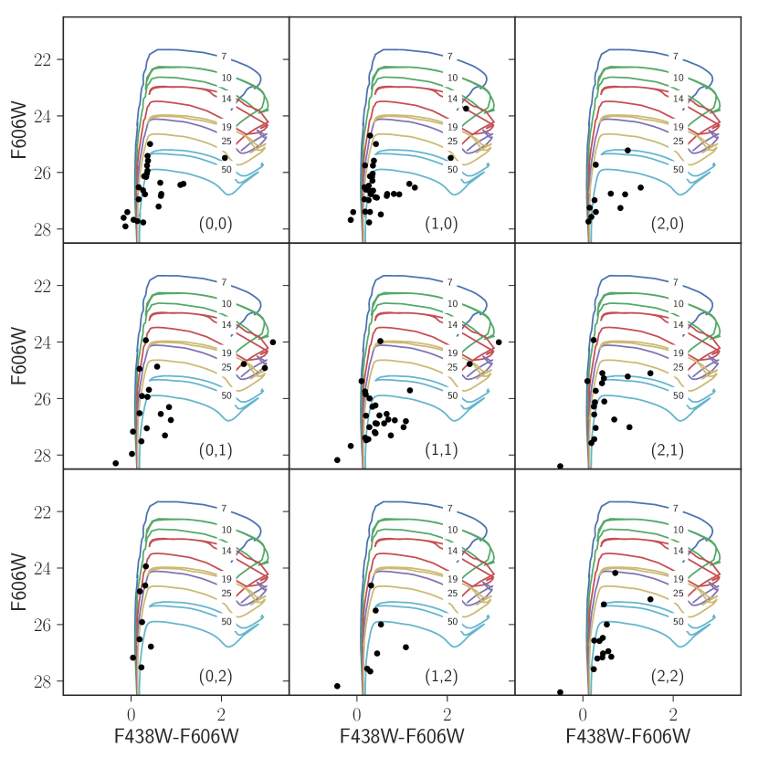
Figure 5: The F438W-F606W CMD for the nine regions near the vanisher. The progenitor could have been born in a neighboring region. To estimate the likelihood of this, we calculate the SFH for the eight regions surrounding the location of the vanisher (central panel). The central region has the highest number of bright MS stars, suggesting that it will have the largest and youngest SFR.

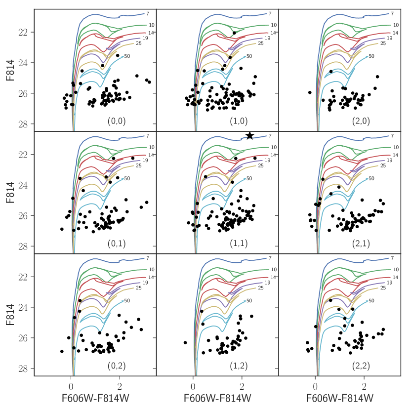
Figure 6: The F606W-F814W CMD for the nine regions near the vanisher. The star in the central panel is the vanisher, N6946-BH1. This star is the brightest red star in all regions, a region that is a couple hundred pc on a side. In fact, there is no star as bright as the vanisher for 300 pc.

Figure 7 shows the SFR as a function of age for each region. Each panel also shows the total stellar mass formed in the last 50 Myr. As supported by the CMDs, the most prominent burst of star formation is the youngest burst in the central region. Therefore, that burst’s age is also the most likely age of the progenitor.

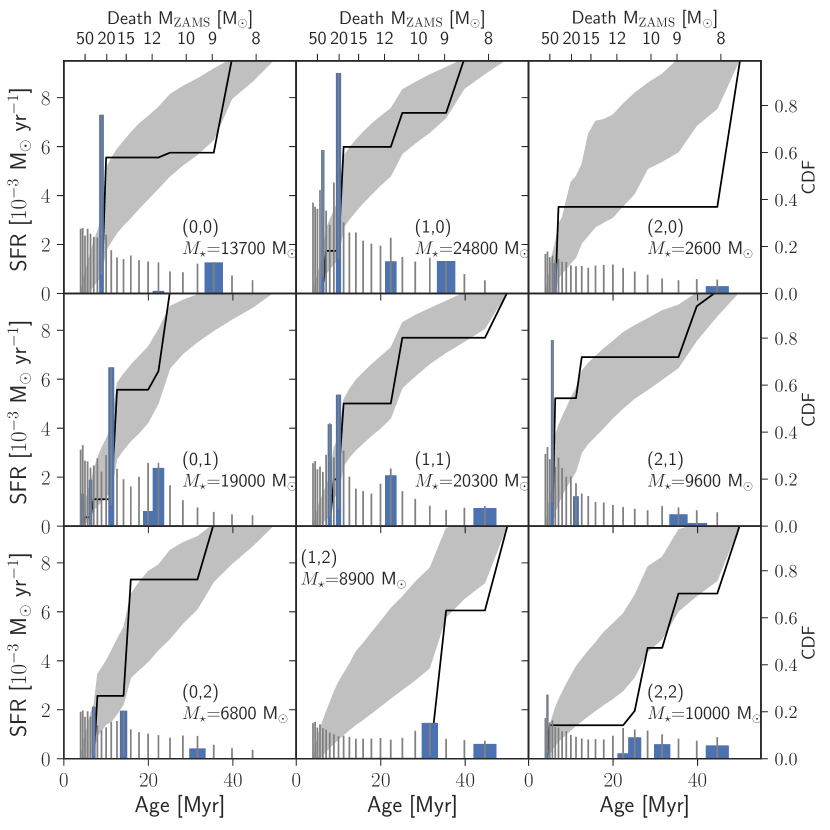
Figure 7: The SFHs for the nine regions near the vanisher. These plots show both the SFR (blue bars) and the cumulative distribution in the last 50 Myr. Each panel also shows the total amount of stars formed ($M_{\star}$) in that region in the last 50 Myr. The central region has the most prominent young burst of star formation and the most stars formed. While there is a possibility that the vanisher was born in association with other stars and kicked to this region, the intensity of recent star formation associated with the central region suggests that the vanisher was born with the stars of the central region.

Figure 8 shows the probability distribution for each region’s age. The PDF in the central panel is normalized to one. All other regions are renormalized by the ratio of their total stellar mass ($M_{\star}$) to the central region’s $M_{\star}$. This gives a visual representation of which regions are most likely associated with the progenitor. Again, the central region has the most recent and vigorous recent SF, which reflects the fact that the central region contains the most number of young MS stars. The other regions have too few stars to really constrain their ages well. In summary, because the central panel has the largest number of young stars, reporting the age and inferred mass from the central panel most likely represents the age of the progenitor, including any possibility for dispersion or kicks.

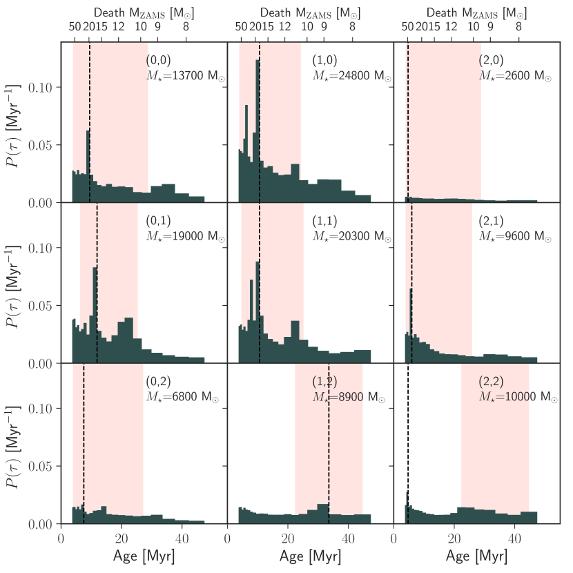
Figure 8: Marginalized age distributions for the nine regions surrounding the vanisher. The dashed line in each panel shows the most likely age, the rose vertical band highlights the narrowest 68% CI, and $M_{\star}$ indicates the total stellar mass formed in the last 50 Myr. The central panel is normalized to one, and the other eight are renormalized by the total mass of stars formed in that region compared to the central region. The central region contains the most young stars and has the youngest most likely age.

3.1 Comparison with SED-fitting Results

N6946-BH1 offers a unique opportunity to compare the SED-fitting and age-dating methods.

From SED fitting, Adams et al. (2017) infer a progenitor mass of $25^{+2}_{-1}$ $M_{\odot}$. With the more accurate TRGB-derived distance, the SED-derived mass becomes $27^{+2}_{-1}$ $M_{\odot}$ (the vertical black bar in Figure 3). Formally, they derived an uncertainty that is quite small, but this uncertainty in mass only accounts for the relatively small random uncertainty in the photometry of the progenitor. However, the last stages of stellar evolution are the most difficult to model, and so the systematic uncertainties associated with modeling the SED are likely much larger. For example, Beasor & Davies (2016, 2018) found that a combination of significant mass loss, dust formation, and/or extreme bolometric correction in the last stages of red supergiants (RSGs) can dramatically reduce the flux in the most easily accessible visible and near IR bands. Hence, the SED-to-progenitor mass mapping can be quite uncertain.

It is also not entirely clear that the progenitor would be in hydrostatic equilibrium just before collapse. The relative steadiness of the progenitor’s luminosity (Adams et al., 2017) supports that the progenitor was likely in a hydrostatic state, but this is not entirely certain. Theoretical models suggest that there is a great deal of convective energy in the cores, enough to unbind the outer envelope if that energy can couple efficiently (Quataert & Shiode, 2012; Fuller, 2017).

The observed CMD is consistent with a population with an age of $10.6^{+14.5}_{-5.9}$ Myr. Within the assumption of single-star evolution, this age corresponds to an initial mass of $17.9^{+29.9}_{-7.6}$ $M_{\odot}$. By contrast, the SED-derived mass, $\sim$27 $M_{\odot}$, experiences core collapse at 7 Myr (Marigo et al., 2017) (7.6 Myr for the SED-derived mass, $\sim$24, from the rotating models). Formally, these ages and masses are consistent within our uncertainties. If the progenitor is truly associated with the burst at $\sim$10 Myr, then the most likely age either requires an $\sim$27 $M_{\odot}$ progenitor to live 40% longer than standard evolution theories predict or an $\sim$18 $M_{\odot}$ progenitor must have a luminosity 2.5 times brighter than predicted just before collapse. This discrepancy could be explained by either binary evolution or episodic eruptions at the end of the progenitor’s life.

Unfortunately, in the central 100 pc, there are only a handful of bright MS stars to constrain the age of the stellar population. As a result, while the best-fit SFH does not show any populations younger than 10 Myr, $91\%$ of the age PDF (Figure 3) has ages older than 7 Myr, making the brightness of the progenitor marginally consistent with the age PDF of the surrounding stars. In this case, standard single-star evolutionary models may be appropriate in describing the fate of the progenitor.

3.2 N6946-BH1 in the Context of Core-collapse Progenitor Theory and Observations

In general, theory predicts that the explodability of a star depends upon these parameters: the neutron star mass ($M_{\rm NS}$), neutron star radius ($R_{\rm NS}$), the neutrino luminosity ($L_{\nu}$), and the amount of mass accreting during collapse ($\dot{\mathcal{M}}$) (Murphy & Dolence, 2017). In the context of these important parameters, there is a critical hypersurface that divides nonexploding and explosive solutions. During collapse, these parameters evolve over time, and if the evolution crosses the critical threshold, then the star explodes. The progenitor’s structure prior to collapse likely determines the evolution in these parameters and whether the evolution crosses the critical hypersurface for explosion. To date, there is no direct mapping between the progenitor structure and whether the evolution crosses the critical hypersurface. However, there are many studies exploring more approximate explodability conditions (Burrows & Goshy, 1993; Janka, 2001; Murphy & Burrows, 2008; O’Connor & Ott, 2011; Ugliano et al., 2012; Ertl et al., 2016; Müller et al., 2016; Sukhbold et al., 2016).

In one such study, Sukhbold et al. (2016) explored the explodability of progenitors from 9 to 120 $M_{\odot}$; they found a general trend that the least massive stars explode more easily, but they also found that the explodability may not be entirely monotonic with mass. More specifically, they found islands of SN production. Generically, their simulations indicate that all masses below 15 $M_{\odot}$ explode. Above this mass, there are islands of failed explosions and BH formation. The existence of these islands seems to be robust to the details of stellar evolution assumptions, but the size and frequency of these islands depends upon progenitor prescription. For typical stellar evolution assumptions, the region between 15 and 22 $M_{\odot}$ shows both explosions and failed explosions. Between 22 and 25 $M_{\odot}$, there seems to be a robust region of failed SNe. Above 28 $M_{\odot}$ most models fail to explode. Considering all results, the minimum progenitor to exhibit a failed SN is 15 $M_{\odot}$. This prediction is consistent with our best-fit progenitor mass for N6946-BH1, $17.9^{+29.9}_{-7.6}$ $M_{\odot}$.

If the explodability mostly depends upon the progenitor’s initial mass, then constraining the progenitor distribution of SNe could constrain the the progenitor distribution of failed SNe. For example, Smartt (2015) constrained the progenitor distribution for 18 SNe IIP (plus 27 upper limits on progenitors). Assuming a Salpeter mass function, they found a minimum mass of $9.5^{+0.5}_{-2}$ $M_{\odot}$ and a maximum mass of $16.5^{2.5}_{-2.5}$ $M_{\odot}$. This maximum mass for SNe IIP is consistent with the theoretical minimum mass for failed SNe. It is also consistent with our best-fit mass for N6946-BH1. However, one should note that the maximum mass for SNe IIP may not be the maximum mass for explosion. Progenitors above this mass may explode as other types of SNe. Complicating this interpretation, Davies & Beasor (2018) recently reanalyzed the progenitor masses of the SNe IIP using bolometric corrections that are derived from very red supergiants near death. With these new bolometric corrections, they found a higher upper mass ($19.0^{+2.5}_{-1.3}$ $M_{\odot}$) for the progenitor masses of SNe IIP.

The distribution of masses from the age-dating technique does not show a maximum mass for explosion. However, the distributions are consistent with the most massive stars failing to explode more often than the least massive stars. Williams et al. (2018) age-dated the stellar populations for 25 SNe and found a distribution of median masses that is consistent with a wide range of masses. However, all 25 SNe have uncertainties that extend below 18 $M_{\odot}$, so the masses are also consistent with lower masses exploding and higher masses failing to explode. Díaz-Rodríguez et al. (2018) inferred the progenitor mass distribution for 94 SNRs. They found a very well-constrained minimum mass ($7.33^{+0.02}_{-0.16}$ $M_{\odot}$) and a power-law slope that is steeper than Salpeter ($-2.96^{+0.45}_{-0.25}$) but a maximum mass that is $>$59 $M_{\odot}$. While the maximum mass is well above the best-fit mass for N6946-BH1, the steeper-than-Salpeter (-2.35) slope could suggest that the most massive stars explode less frequently.

Both observations and theory of SN progenitors suggest that the least massive stars tend to explode more readily than the most massive stars. This implies that the most massive stars are more likely to form black holes by a failed supernova. Our best-fit mass of N6946-BH1 is consistent with this general trend.

4 Conclusion

The vanishing star, N6946-BH1, is the first BH formation candidate and provides the first constraints on which stars fail to explode and form BHs. Using stellar evolution models, Adams et al. (2017) modeled the SED and inferred an $M_{\rm ZAMS}$ of $\sim$25. These SED-to-progenitor mass mappings rely on modeling the most uncertain stage of stellar evolution: the last stage. The accuracy of these models could be dramatically affected by circumstellar dust obscuration, extreme mass loss, or extreme bolometric corrections (Beasor & Davies, 2018; Davies & Beasor, 2018), or even a violation of hydrostatic equilibrium (Quataert & Shiode, 2012; Fuller, 2017). In either case, these uncertainties are difficult to model and quantify, making it important to constrain the progenitor mass with another technique.

We age-date the surrounding stellar population, which is most sensitive to modeling the MS and helium-burning phases; both are more certain phases of stellar evolution. We find a progenitor age of $10.6^{+14.5}_{-5.9}$ Myr and an $M_{\rm ZAMS}$ of $17.9^{+29.9}_{-7.6}$ $M_{\odot}$. Even though the best-fit age-derived and the SED-derived masses differ, formally, the SED-derived mass falls within the 68% CI of the age-derived mass. We find that $91\%$ of our PDF lies below this mass, hinting at a slight tension between the age and the direct-imaging result.

To infer the age, MATCH models the magnitude and color of stars; a fundamental parameter in modeling magnitudes is the distance. We use a Bayesian maximum-likelihood method to fit for the TRGB (Makarov et al., 2006; McQuinn et al., 2016). We find a distance modulus of $m-M=29.47\pm 0.079$, which corresponds to $7.83\pm 0.29$ Mpc.

The primary systematic and modeling uncertainties that affect the age-dating method are binary evolution and runaway stars. Mergers and mass transfer modify both the mass and stellar lifetimes in a way that is inconsistent with the predictions of single-star stellar evolution. If the progenitor of N6946-BH1 was a runaway star, then the age of the nearby stars may not be coeval. However, we derived the SFHs for eight regions within a 100 pc, but we find that the region colocated with the vanisher has the youngest and most active recent star formation. This result suggests that the vanisher is not a runaway star. On the other hand, the slight difference between the most likely age and the SED-derived mass hints that binary evolution may have played a role in the progenitor of N6946-BH1. But, once again, the SED-derived mass is only marginally inconsistent with the age-derived mass.

In summary, the age of the BH formation candidate, N6946-BH1, was likely $10.6^{+14.5}_{-5.9}$ Myr. Assuming single-star evolution, this age corresponds to a star with a mass of $17.9^{+29.9}_{-7.6}$ $M_{\odot}$ at birth. To better constrain the age and uncertainty will require photometry that includes more stars in association. This will happen in one of three ways. One, a larger optical, UV, and IR space telescope will provide more MS stars. Two, we are lucky, and a failed SN occurs in a closer galaxy. Three, the region surrounding N6946-BH1 is remarkably sparse. If the next BH formation candidate, occurs in a more populated region, then it might be possible to have a larger sample of main sequence stars to constrain the age. In any case, the next BH-formation candidate could better constrain the progenitor and any differences between the techniques.

References

- Adams et al. (2017) Adams, S. M., Kochanek, C. S., Gerke, J. R., Stanek, K. Z., & Dai, X. 2017, MNRAS, 468, 4968
- Aghakhanloo et al. (2017) Aghakhanloo, M., Murphy, J. W., Smith, N., & Hložek, R. 2017, MNRAS, 472, 591
- Beasor & Davies (2016) Beasor, E. R., & Davies, B. 2016, MNRAS, 463, 1269
- Beasor & Davies (2018) —. 2018, MNRAS, 475, 55
- Bruenn et al. (2016) Bruenn, S. W., Lentz, E. J., Hix, W. R., et al. 2016, ApJ, 818, 123
- Burrows & Goshy (1993) Burrows, A., & Goshy, J. 1993, ApJ, 416, L75
- Burrows et al. (2018) Burrows, A., Vartanyan, D., Dolence, J. C., Skinner, M. A., & Radice, D. 2018, Space Sci. Rev., 214, doi:10.1007/s11214-017-0450-9
- Cardelli et al. (1989) Cardelli, J. A., Clayton, G. C., & Mathis, J. S. 1989, ApJ, 345, 245
- Carretta et al. (2000) Carretta, E., Gratton, R. G., Clementini, G., & Fusi Pecci, F. 2000, ApJ, 533, 215
- Davies & Beasor (2018) Davies, B., & Beasor, E. R. 2018, MNRAS, 474, 2116
- Díaz-Rodríguez et al. (2018) Díaz-Rodríguez, M., Murphy, J. W., Rubin, D. A., et al. 2018, ArXiv e-prints, arXiv:1802.07870
- Dolphin (2002a) Dolphin, A. E. 2002a, MNRAS, 332, 91
- Dolphin (2002b) —. 2002b, MNRAS, 332, 91
- Dolphin (2012) —. 2012, ApJ, 751, 60
- Dolphin (2013) —. 2013, ApJ, 775, 76
- Eldridge et al. (2011) Eldridge, J. J., Langer, N., & Tout, C. A. 2011, MNRAS, 414, 3501
- Ertl et al. (2016) Ertl, T., Janka, H.-T., Woosley, S. E., Sukhbold, T., & Ugliano, M. 2016, ApJ, 818, 124
- Fuller (2017) Fuller, J. 2017, MNRAS, 470, 1642
- Gerke et al. (2015) Gerke, J. R., Kochanek, C. S., & Stanek, K. Z. 2015, MNRAS, 450, 3289
- Gogarten et al. (2009) Gogarten, S. M., Dalcanton, J. J., Murphy, J. W., et al. 2009, ApJ, 703, 300
- Janka (2001) Janka, H.-T. 2001, A&A, 368, 527
- Jennings et al. (2012) Jennings, Z. G., Williams, B. F., Murphy, J. W., et al. 2012, ApJ, 761, 26
- Jennings et al. (2014) —. 2014, ApJ, 795, 170
- Karachentsev et al. (2000) Karachentsev, I. D., Sharina, M. E., & Huchtmeier, W. K. 2000, A&A, 362, 544
- Kochanek et al. (2008) Kochanek, C. S., Beacom, J. F., Kistler, M. D., et al. 2008, ApJ, 684, 1336
- Mabanta & Murphy (2018) Mabanta, Q. A., & Murphy, J. W. 2018, ApJ, 856, 22
- Makarov et al. (2006) Makarov, D., Makarova, L., Rizzi, L., et al. 2006, AJ, 132, 2729
- Marigo et al. (2017) Marigo, P., Girardi, L., Bressan, A., et al. 2017, ApJ, 835, 77
- Maund (2017) Maund, J. R. 2017, MNRAS, 469, 2202
- McQuinn et al. (2016) McQuinn, K. B. W., Skillman, E. D., Dolphin, A. E., Berg, D., & Kennicutt, R. 2016, ApJ, 826, 21
- Melson et al. (2015) Melson, T., Janka, H.-T., & Marek, A. 2015, ApJ, 801, L24
- Müller et al. (2016) Müller, B., Heger, A., Liptai, D., & Cameron, J. B. 2016, MNRAS, 460, 742
- Murphy & Burrows (2008) Murphy, J. W., & Burrows, A. 2008, ApJ, 688, 1159
- Murphy & Dolence (2017) Murphy, J. W., & Dolence, J. C. 2017, ApJ, 834, 183
- Murphy et al. (2011) Murphy, J. W., Jennings, Z. G., Williams, B., Dalcanton, J. J., & Dolphin, A. E. 2011, ApJ, 742, L4
- O’Connor & Ott (2011) O’Connor, E., & Ott, C. D. 2011, ApJ, 730, 70
- O’Donnell (1994) O’Donnell, J. E. 1994, ApJ, 422, 158
- Oh et al. (2015) Oh, S., Kroupa, P., & Pflamm-Altenburg, J. 2015, ApJ, 805, 92
- Quataert & Shiode (2012) Quataert, E., & Shiode, J. 2012, MNRAS, 423, L92
- Radice et al. (2017) Radice, D., Burrows, A., Vartanyan, D., Skinner, M. A., & Dolence, J. C. 2017, ApJ, 850, 43
- Reynolds et al. (2015) Reynolds, T. M., Fraser, M., & Gilmore, G. 2015, MNRAS, 453, 2885
- Rizzi et al. (2007) Rizzi, L., Tully, R. B., Makarov, D., et al. 2007, ApJ, 661, 815
- Roberts et al. (2016) Roberts, L. F., Ott, C. D., Haas, R., et al. 2016, ArXiv e-prints, arXiv:1604.07848
- Schlafly & Finkbeiner (2011) Schlafly, E. F., & Finkbeiner, D. P. 2011, ApJ, 737, 103
- Smartt (2009) Smartt, S. J. 2009, ARA&A, 47, 63
- Smartt (2015) —. 2015, PASA, 32, e016
- Sukhbold et al. (2016) Sukhbold, T., Ertl, T., Woosley, S. E., Brown, J. M., & Janka, H.-T. 2016, ApJ, 821, 38
- Sukhbold et al. (2017) Sukhbold, T., Woosley, S., & Heger, A. 2017, ArXiv e-prints, arXiv:1710.03243
- Tikhonov (2014) Tikhonov, N. A. 2014, Astronomy Letters, 40, 537
- Ugliano et al. (2012) Ugliano, M., Janka, H.-T., Marek, A., & Arcones, A. 2012, ApJ, 757, 69
- Williams et al. (2018) Williams, B. F., Hillis, T. J., Murphy, J. W., et al. 2018, ArXiv e-prints, arXiv:1803.08112
- Williams et al. (2014a) Williams, B. F., Peterson, S., Murphy, J., et al. 2014a, ApJ, 791, 105
- Williams et al. (2014b) Williams, B. F., Lang, D., Dalcanton, J. J., et al. 2014b, ApJS, 215, 9
- Woosley et al. (2002) Woosley, S. E., Heger, A., & Weaver, T. A. 2002, Reviews of Modern Physics, 74, 1015