Casimir force in dense confined electrolytes

Abstract

Understanding the force between charged surfaces immersed in an electrolyte solution is a classic problem in soft matter and liquid-state theory. Recent experiments showed that the force decays exponentially but the characteristic decay length in a concentrated electrolyte is significantly larger than what liquid-state theories predict based on analysing correlation functions in the bulk electrolyte. Inspired by the classical Casimir effect, we consider an alternative mechanism for force generation, namely the confinement of density fluctuations in the electrolyte by the walls. We show analytically within the random phase approximation, which assumes the ions to be point charges, that this fluctuation-induced force is attractive and also decays exponentially, albeit with a decay length that is half of the bulk correlation length. These predictions change dramatically when excluded volume effects are accounted for within the mean spherical approximation. At high ion concentrations the Casimir force is found to be exponentially damped oscillatory as a function of the distance between the confining surfaces. Our analysis does not resolve the riddle of the anomalously long screening length observed in experiments, but suggests that the Casimir force due to mode restriction in density fluctuations could be an hitherto under-appreciated source of surface-surface interaction.

I Introduction

Understanding the structure, phase behaviour and dynamics of ionic liquids and concentrated electrolytes, both in the bulk and near interfaces, is a longstanding challenge. Since the pioneering work of Helmholtz helmholtz1853 , Debye and Hückel debye1923 , Onsager onsager1934deviations and many others, much recent progress has been made using the statistical mechanics tools of the theory of classical liquids hansen2013theory . A large body of “exact” results and sum-rules was established martin1988sum , while the Ornstein-Zernike (OZ) formalism ornstein1914accidental and classical density functional theory percus1962approximation became the basis of numerous approximate theories of the structure, including non-linear integral equations for the pair correlation functions hansen2013theory ; amongst these theories the mean spherical approximation (MSA) plays an important role, since it allows for analytic solutions of simple, semi-realistic models of ionic liquids waisman1972mean ; waisman1972mean1 , which will be used in the present paper. The OZ formalism was also put to good use to examine the asymptotic decay of pair correlation functions and density profiles at interfaces attard1993asymptotic ; leote1994decay ; attard1996electrolytes . Although different analytical or numerical theories predict different dependences of the correlation (or screening) length on ion concentration, the theoretical predictions converge on two qualitative features: (1) the decay of the correlation is exponential; and (2) the longest correlation length in a concentrated electrolyte is of the same order of magnitude as the (mean) ion diameter.

However, recent experiments suggest an “underscreening” phenomenon, namely the existence of an anomalously large decay length which is incongruent with the above mentioned theoretical predictions gebbie2013ionic ; gebbie2015long ; smith2016electrostatic . Surface force balance experiments reveal hat the force acting between negatively charged mica surfaces immersed in an electrolyte decays exponentially with surface separation $L$, but the decay (or screening) length $\lambda_{S}$ scales as lee2017scaling :

$$\frac{\lambda_{S}}{\lambda_{D}}\sim\begin{cases}1,&a/\lambda_{D}\ll 1\\ (a/\lambda_{D})^{3},&a/\lambda_{D}\gg 1,\end{cases}$$ (1)

with

$$\lambda_{D}=\frac{1}{\sqrt{4\pi l_{B}(\rho_{+}z_{+}^{2}+\rho_{-}z_{-}^{2})}}$$ (2)

the Debye length, $\rho_{\pm}$ ($z_{\pm}$) the number density (valence) of the cations/anions, $a$ the ionic radius, while $l_{B}=e^{2}/(4\pi\epsilon\epsilon_{0}k_{B}T)$ is the Bjerrum length with $\epsilon$ the dielectric constant of the electrolyte, which depends on ion concentration This scaling relation has been verified for various electrolyte chemistries, ranging from pure ionic liquids (e.g. room temperature molten salts) and ionic liquid-organic solvent mixtures to aqueous alkali halide solutions. A scaling theory has been proposed, based on identifying solvent molecules as effective charge carriers, with an effective charge determined by thermal fluctuations lee2017scaling ; lee2017underscreening . More recently, a first-principles analysis based on Landau fluctuation theory and the MSA has been put forward, which confirms that $\lambda_{S}/\lambda_{D}$ has a power law dependence on $a/\lambda_{D}$, albeit with a considerably smaller exponent compared to the experimental findings summarised in Equation (1) rotenberg2017underscreening .

In this paper, we explore an additional mechanism of force generation in confined systems, namely the classical counterpart of the celebrated quantum Casimir effect of an electromagnetic field fluctuation-induced force acting between the confining surfaces casimir1948attraction . The classical Casimir effect is observed in high temperature confined systems, where the thermal fluctuations now play the role of quantum field fluctuations. Restrictions on the possible Fourier components (or modes) of thermal fluctuations imposed by spatial confinement generate the classical Casimir force. Large amplitude critical fluctuations in a fluid close to a thermodynamic critical point strongly enhance the classical Casimir effect, where the universality of critical scaling laws entails a corresponding universality of the Casimir force fisher1978 (for a recent review of the classical Casimir force, see gambassi2009casimir ).

We examine the possibility of an observable Casimir force in confined ionic fluids under conditions inspired by the aforementioned experimental setups gebbie2013ionic ; gebbie2015long ; smith2016electrostatic . No critical fluctuations are involved, but the infinite range of the Coulombic interactions is expected to significantly affect the resulting Casimir force. This question has already been explored in the high temperature limit within Debye-Hückel theory of point ions, for a variety of boundary conditions, and using a microscopic description of the confining metallic or dielectric media jancovici2004screening ; jancovici2005casimir ; buenzli2005casimir ; hoye2009casimir .

This paper describes an attempt to go beyond the point ion description by considering finite size ions to account for excluded volume effects which are crucial for concentrated electrolytes. In Section II, we first consider the point ion limit using a systematic approach inspired by a paper dealing with Casimir force in confined non-equilibrium systems brito2007generalized , while excluded volume effects are included within the MSA in Section III. Some concluding remarks are made in Section IV.

II The free energy of fluctuation modes

We begin our analysis by expressing the free energy in terms of fluctuation modes. Let $F=F(\rho_{+},\rho_{-})$ be the free energy of a bulk electrolyte with cation density $\rho_{+}$ and anion density $\rho_{-}$. We expand around the mean density, i.e. $\rho_{\alpha}=\rho_{\alpha}^{0}+\delta\rho_{\alpha}$, and write

$$F=F(\rho_{+}^{0},\rho_{-}^{0})+\sum_{\alpha=\pm}\delta\rho_{\alpha}\frac{\partial F}{\partial\rho_{\alpha}}\Bigg{|}_{\rho_{+}^{0},\rho_{-}^{0}}+\frac{1}{2}\sum_{\alpha,\beta=\pm}\delta\rho_{\alpha}\delta\rho_{\beta}\frac{\partial^{2}F}{\partial\rho_{\alpha}\partial\rho_{\beta}}\Bigg{|}_{\rho_{+}^{0},\rho_{-}^{0}}$$ (3)

Defining $\Delta F=F-F(\rho_{+}^{0},\rho_{-}^{0})$, and noting that $\left<\delta\rho_{\alpha}\right>=0$, where $\left<\cdot\right>$ denotes thermal average, we obtain

$$\Delta F=\frac{1}{2}\sum_{\alpha,\beta=\pm}\left<\delta\rho_{\alpha}\delta\rho_{\beta}\right>\frac{\partial^{2}F}{\partial\rho_{\alpha}\partial\rho_{\beta}}\Bigg{|}_{c_{+}^{0},c_{-}^{0}}=\frac{1}{2}\sum_{\alpha,\beta=\pm}\left<\delta\rho_{\alpha}\delta\rho_{\beta}\right>\chi^{-1}_{\alpha\beta}$$ (4)

where we have defined the partial response functions rotenberg2017underscreening

$$\frac{\partial^{2}F}{\partial\rho_{\alpha}\partial\rho_{\beta}}\Bigg{|}_{\rho_{+}^{0},\rho_{-}^{0}}=\chi_{\alpha\beta}^{-1}.$$ (5)

We can express the fluctuations in terms of Fourier modes $\delta\rho_{\alpha}(\mathbf{r})=\frac{1}{V}\sum_{\mathbf{k}}e^{-i\mathbf{k}\cdot\mathbf{r}}\delta\rho_{\alpha,\mathbf{k}}$, and the correlations of the fluctuations are related to the structure factors $S_{\alpha\beta}(\mathbf{k})=\left<\delta\rho_{\alpha,\mathbf{k}}\delta\rho_{\beta,\mathbf{-k}}\right>/V$, which are in principle experimentally measurable using techniques such as neutron scattering.

We now consider an electrolyte solution confined between two infinite charged walls separated by a distance $L$. For a strongly charged surface, one might imagine that the concentration fields of the cations and anions are pinned on the surface, or at the very least the surface anchors the fields and significantly reduces the magnitude of fluctuations. Assuming that the fields are pinned at the walls (i.e. $\delta\rho_{\alpha}=0$ at the walls), the wavenumber of the fluctuation modes normal to the surfaces can only take discrete values $k_{n}=n\pi/L$. Therefore, the fluctuation energy inside the slit is given by

$$\Delta F_{\mathrm{in}}=\int\frac{\mathrm{d}^{2}\mathbf{k}}{(2\pi)^{2}}\left[\frac{\pi}{L}\sum_{n=1}^{\infty}\sum_{\alpha,\beta=\pm}\chi^{-1}_{\alpha\beta}S_{\alpha\beta}\left(\sqrt{k^{2}+\left(\frac{n\pi}{L}\right)^{2}}\right)-\int_{0}^{\infty}\mathrm{d}p\sum_{\alpha,\beta=\pm}\chi^{-1}_{\alpha\beta}S_{\alpha\beta}\left(\sqrt{k^{2}+p^{2}}\right)\right]$$ (6)

where we have subtracted the energy in the limit when $L\rightarrow\infty$, and exploited the symmetry of the summand and integrand with respect to negative $n$ and $p$. We note that the $n=0$ term is irrelevant since it is independent of $L$. The resulting Casimir force is simply the derivative of the fluctuation energy with respect to the surface separation

$$f_{\mathrm{Casimir}}=-\frac{\partial\Delta F_{\mathrm{in}}}{\partial L}.$$ (7)

Note that we have implicitly assumed that charged surfaces do not affect the structure factors $S_{\alpha\beta}(k)$ – this assumption restricts the validity of our analysis to the far field limit when the walls are far apart.

Equations (6)-(7) relate the bulk response functions and the structure factors to the Casimir force. We next turn to estimating those quantities for a two-component electrolyte. Following ref. rotenberg2017underscreening , we introduce the wavenumber-dependent partial response functions $\hat{\chi}_{\alpha\beta}$, defined by

$$\hat{\chi}^{-1}_{\alpha\beta}(k)=\frac{\delta_{\alpha\beta}}{\rho_{\alpha}}-\hat{c}_{\alpha\beta}(k),$$ (8)

where $\hat{c}_{\alpha\beta}(k)$ is the Fourier transform of the OZ direct correlation function. Using the definition of the structure factor in terms of the total correlation function $\hat{h}_{\alpha\beta}(k)$

$$S_{\alpha\beta}(k)=\rho_{\alpha}\delta_{\alpha\beta}+\rho_{\alpha}\rho_{\beta}\hat{h}_{\alpha\beta}(k)$$ (9)

it can be shown hansen2013theory ; rotenberg2017underscreening that

$$\begin{pmatrix}S_{++}&S_{+-}\\ S_{-+}&S_{--}\end{pmatrix}=\frac{1}{\hat{\chi}^{-1}_{++}\hat{\chi}^{-1}_{--}-\hat{\chi}^{-1}_{+-}\hat{\chi}^{-1}_{-+}}\begin{pmatrix}\hat{\chi}^{-1}_{++}&-\hat{\chi}^{-1}_{+-}\\ -\hat{\chi}^{-1}_{-+}&\hat{\chi}^{-1}_{--}\end{pmatrix}.$$ (10)

To make further progress, we can split the direct correlation functions into the Coulomb part and the short-range part:

$$\hat{c}_{\alpha\beta}(k)=-\frac{4\pi z_{\alpha}z_{\beta}l_{B}}{k^{2}}+\hat{c}^{s}_{\alpha\beta}(k).$$ (11)

The Random Phase Approximation (RPA) assumes that $\hat{c}^{s}_{\alpha\beta}(k)=0$, and in this limit Equation (8) can be substituted into Equation (10) to yield analytical expressions for the structure factors.

The partial response functions, Equation (5), can be evaluated by noting that the free energy density of an electrolyte in the random phase approximation reads

$$\frac{F}{k_{B}TV}=\rho_{+}\left[\log(a^{3}\rho_{+})-1\right]+\rho_{-}\left[\log(a^{3}\rho_{-})-1\right]-\frac{1}{12\pi\lambda_{D}^{3}}.$$ (12)

Taking derivatives with respect to $\rho_{+}$ and $\rho_{-}$, we thus arrive at

$$\chi^{-1}_{\alpha\beta}=Vk_{B}T\left(\frac{\delta_{\alpha\beta}}{\rho_{\alpha}}-\pi\lambda_{D}l_{B}^{2}z^{2}_{\alpha}z^{2}_{\beta}\right)\;.$$ (13)

For a $1:1$ electrolyte, $z_{+}=-z_{-}=1$, $\rho_{+}=\rho_{-}=\rho/2$, and the sum of structure factors can be written as

$$\sum_{\alpha,\beta=\pm}\chi^{-1}_{\alpha\beta}S_{\alpha\beta}\left(k\right) = \frac{Vk_{B}T}{2}\left[\left(2-\frac{l_{B}}{4\lambda_{D}}\right)\frac{2\lambda_{D}^{2}k^{2}+1}{\lambda_{D}^{2}k^{2}+1}-\frac{l_{B}}{4\lambda_{D}}\frac{1}{1+\lambda_{D}^{2}k^{2}}\right]$$ (14)

$$= Vk_{B}T\left(2-\frac{l_{B}}{4\lambda_{D}}-\frac{1}{1+\lambda_{D}^{2}k^{2}}\right)$$

we first note that the constant term drops out of the Casimir force as the sum and the integral cancel out,

$$\sum_{n=1}^{\infty}\frac{\pi}{L}-\int_{0}^{\infty}\mathrm{d}p=\sum_{n=1}^{\infty}\left(\frac{\pi}{L}-\int_{\frac{(n-1)\pi}{L}}^{\frac{n\pi}{L}}\mathrm{d}p\right)=0.$$ (15)

The crucial step of our analysis is to note that

$$\frac{\pi}{L}\sum_{n=1}^{\infty}\frac{1}{1+\lambda_{D}^{2}k^{2}+\lambda_{D}^{2}\left(\frac{n\pi}{L}\right)^{2}}=\frac{\pi}{L}\frac{1}{2(1+\lambda_{D}^{2}k^{2})}\left[\frac{L}{\lambda_{D}}\sqrt{1+\lambda_{D}^{2}k^{2}}\coth\left(\frac{L}{\lambda_{D}}\sqrt{1+\lambda_{D}^{2}k^{2}}\right)-1\right]$$ (16)

and

$$\int_{0}^{\infty}\mathrm{d}p\frac{1}{1+\lambda_{D}^{2}k^{2}+\lambda_{D}^{2}p^{2}}=\frac{\pi}{2\lambda_{D}\sqrt{1+\lambda_{D}^{2}k^{2}}},$$ (17)

Substituting the difference between Equations (16) and (17) into Equation (6), and multiplying by $L$, we obtain the free energy per unit area (instead of volume):

$$\frac{\Delta F_{\mathrm{in}}}{Ak_{B}T}=\frac{1}{4}\left(\int_{0}^{\infty}\frac{k}{1+\lambda_{D}^{2}k^{2}}\mathrm{d}k-L\int_{0}^{\infty}k\frac{\coth\left(\frac{L}{\lambda_{D}}\sqrt{1+k^{2}\lambda_{D}^{2}}\right)-1}{\lambda_{D}\sqrt{1+\lambda_{D}^{2}k^{2}}}\mathrm{d}k\right),$$ (18)

with $A$ the plate area. While the first term of Equation (18) diverges logarithmically, it is $L$-independent and therefore does not contribute to the disjoining force. The second term can be integrated analytically to give

$$\frac{\Delta F_{\mathrm{in}}}{Ak_{B}T}=-\frac{1}{4}\left[\frac{L}{\lambda_{D}^{3}}-\frac{1}{\lambda_{D}^{2}}\log\left(2\sinh\frac{L}{\lambda_{D}}\right)\right].$$ (19)

Therefore, the Casimir force per unit area is

$$\frac{f_{\mathrm{Casimir}}}{A}=\frac{k_{B}T}{4\lambda_{D}^{3}}\left(1-\coth\frac{L}{\lambda_{D}}\right).$$ (20)

Perhaps surprisingly, Equation (20) reveals that the Casimir force is attractive, and has an asymptotic decay length of of $\lambda_{D}/2$.

III Hard core repulsion and the Mean-Spherical Approximation

The RPA ignores hard-core interactions and assumes point-like ions. This approximation is unreasonable in dense ionic systems such as ionic liquids and concentrated electrolytes. To include hard-core interactions, we consider the Mean Spherical Approximation (MSA). The MSA direct correlation function for a two component hard sphere electrolyte with cations and anions having equal diameters $\sigma$ has been derived in pioneering papers wertheim1963exact ; thiele_equation_1963 ; waisman1972mean ; waisman1972mean1 , and reads

$$\hat{c}^{s}_{\alpha\beta}(k) =\frac{4\pi\sigma^{3}}{(k\sigma)^{6}}\left[24d_{\alpha\beta}-2b_{\alpha\beta}(k\sigma)^{2}+e_{\alpha\beta}(k\sigma)^{4}\right.$$

$$-\left\{24d_{\alpha\beta}-2(b_{\alpha\beta}+6d_{\alpha\beta})(k\sigma)^{2}+(a_{\alpha\beta}+b_{\alpha\beta}+d_{\alpha\beta}+e_{\alpha\beta})(k\sigma)^{4}\right\}\cos(k\sigma)$$

$$\left.+\left\{-24d_{\alpha\beta}(k\sigma)+(a_{\alpha\beta}+2b_{\alpha\beta}+4d_{\alpha\beta})(k\sigma)^{3}\right\}\sin(k\sigma)\right]$$ (21)

where

$$a_{\alpha\beta}=-\frac{(1+2\eta)^{2}}{(1-\eta)^{4}}-2B\left(\frac{\sigma}{\lambda_{D}}\right)\frac{l_{B}}{\sigma}z_{\alpha}z_{\beta},$$

$$b_{\alpha\beta}=-\frac{6\eta(1+\frac{\eta}{2})^{2}}{(1-\eta)^{4}}+\left[B\left(\frac{\sigma}{\lambda_{D}}\right)\right]^{2}\frac{l_{B}}{\sigma}z_{\alpha}z_{\beta},$$

$$d_{\alpha\beta}=-\frac{\eta(1+2\eta)^{2}}{2(1-\eta)^{4}},$$

$$e_{\alpha\beta}=\frac{l_{B}}{\sigma}z_{\alpha}z_{\beta},$$

$$B(x)=\frac{x^{2}+x-x\sqrt{1+2x}}{x^{2}},$$

with $\eta=(\pi/6)\sum_{\alpha}\rho_{\alpha}\sigma^{3}$ the total packing fraction. Substituting Equation (21) into Equation (11) yields the full direct correlation function. Unlike the RPA, the hard core repulsion causes the MSA structure factor to be oscillatory and to decay to zero in the $k\rightarrow\infty$ limit.

To proceed further, we first evaluate numerically the difference between the sum and the integral

$$G_{\alpha\beta}(k_{\parallel},L)=\frac{\pi}{L}\left(\sum_{n=1}^{\infty}S_{\alpha\beta}\left(\sqrt{k_{\parallel}^{2}+\frac{n\pi}{L}}\right)-\int_{0}^{\infty}\;S_{\alpha\beta}\left(\sqrt{k_{\parallel}^{2}+\frac{n\pi}{L}}\right)\mathrm{d}n\right).$$ (22)

and note that both the sum and the integral are convergent since the structure factors decay asymptotically as:

$$\sigma^{3}S_{\alpha\beta}(k)\sim\frac{3\eta}{\pi}\delta_{\alpha\beta}-\frac{36\eta^{2}}{\pi}(a_{\alpha\beta}+b_{\alpha\beta}+d_{\alpha\beta}+e_{\alpha\beta})\frac{\cos(k\sigma)}{(k\sigma)^{2}},\;\mathrm{when}\;k\rightarrow\infty.$$ (23)

and we showed in Equation (15) that a constant term has no bearing on the Casimir force and can be ignored. Using the Euler-Maclaurin formula, we can expand $G_{\alpha\beta}(k_{\parallel},L)$ asymptotically in $1/L$:

$$G_{\alpha\beta}(k_{\parallel},L)=-\frac{1}{2}\frac{\pi}{L}S_{\alpha\beta}\left(k_{\parallel}\right)+o(L^{-1}).$$ (24)

Since the relevant quantity is the Casimir energy per unit area, we need to multiply Equation (22) by $L$ at the end of the calculation, such that the first term in (24) becomes actually a (diverging) constant independent of $L$ (c.f. the first term in Equation (18)). As such, we must subtract it before numerically integrating over $k_{\parallel}$. All in all, the Casimir energy (per unit volume) reads

$$E_{\mathrm{Casimir}}(L)=\sum_{\alpha\beta}\chi_{\alpha\beta}^{-1}F_{\alpha\beta}(L)$$ (25)

where

$$F_{\alpha\beta}(L)=\frac{1}{(2\pi)^{2}}\int_{0}^{\infty}2\pi k_{\parallel}\left[G_{\alpha\beta}(k_{\parallel},L)+\frac{1}{2L}S_{\alpha\beta}\left(k_{\parallel}\right)\right]\mathrm{d}k_{\parallel}$$ (26)

and

$$\chi^{-1}_{\alpha\beta} =\chi^{-1}_{\alpha\beta,RPA}+\hat{c}^{s}_{\alpha\beta}(0)$$

$$=Vk_{B}T\left[\frac{\delta_{\alpha\beta}}{\rho_{\alpha}}-\pi\lambda_{D}l_{B}^{2}z^{2}_{\alpha}z^{2}_{\beta}-\frac{\pi}{3}\sigma^{3}(4a_{\alpha\beta}+3b_{\alpha\beta}+2d_{\alpha\beta}+6e_{\alpha\beta})\right].$$ (27)

We note that although the structure factor has a slow $\cos(k\sigma)/(k\sigma)^{2}$ decay, the integrand $G_{\alpha\beta}(k_{\parallel},L)+\frac{1}{2L}S_{\alpha\beta}\left(k_{\parallel}\right)$ decays rapidly with $k_{\parallel}$, making the numerical integration in Equation (26) particularly easy. We also note that the integral over $k_{\parallel}$ must be performed last since the divergent part needs to be subtracted off by exploiting the asymptotic expansion of the difference between a Riemann sum and the integral provided by the Euler-Maclaurin formula. Finally, the force per unit area is obtained by numerically differentiating Equation (25) with respect to $L$.

As an illustration, we consider aqueous sodium chloride solutions, and use the ion diameter and dielectric constant estimates from ref smith2016electrostatic . Figure 1 shows that the predicted Casimir force as a function of surface separation is attractive for low concentration, confirming the RPA result, but oscillates between attraction and repulsion as a function of surface separation for concentrated electrolytes. Figure 1b shows that the decay length close to saturation concentration is still comparable to the ion diameter, and at 4.9 M the screening length is $\approx 0.32\sigma$, well below experimentally measured values smith2016electrostatic .

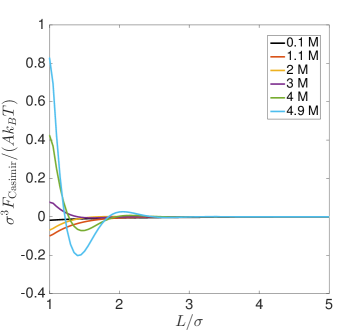
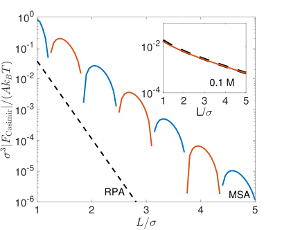
Figure 1: The electrolyte Casimir force for concentrated electrolytes oscillates between attraction and repulsion as a function of surface separation due to hard core repulsion. (a) The predicted electrolyte Casimir force for aqueous sodium chloride solutions. The ion diameter and dielectric constant estimates are taken from ref smith2016electrostatic . (b) The main panel shows the electrolyte Casimir force at 4.9M, a concentration close to saturation, plotted on a log scale. The blue (red) portions denote repulsion (attraction), while the dashed line indicates the RPA result at the same concentration. The inset shows the Casimir force at 0.1M.

IV Conclusion

We have used a second order expansion of the free energy of a binary ionic liquid, confined between two charged insulating surfaces, in powers of the fluctuating ion density modes, for a given spacing $L$ between the surfaces. The resulting Casimir force acting between the surfaces is the derivative of this free energy with respect to $L$ (cf. Equation (7)). The required input is provided by the partial structure factors $S_{\alpha\beta}(k)$. We have examined two cases:

• When the ions are assumed to be point charges, which amounts to the RPA, valid for very low ion concentrations only, the calculations can be carried out analytically, leading to the result in Equation (20); the Casimir force is attractive, and decreases with a decay length equal to one half the Debye length. This prediction agrees with earlier calculations based on a different, fully microscopic Debye-Hückel approach jancovici2004screening ; jancovici2005casimir ; buenzli2005casimir .

• At higher concentrations, finite size (excluded volume) effects become predominant; we have included them within the MSA, which includes a short-range contribution to the partial direct correlation functions, as shown in Equation (21). The resulting expressions for the free energy and Casimir force must now be evaluated numerically. The results for concentrated aqueous NaCl solutions, within an implicit solvent model of oppositely charged hard spheres, are summarized in Fig. 1. Instead of the exponential decay of the Casimir force predicted by the RPA (point charges), the force now exhibits a striking, exponentially damped oscillatory decay as a function of $L$ at the highest, physically relevant concentrations. The periodicity of the oscillations is comparable to the mean ion diameter, reflecting the structural ordering of the ions. To the best of our knowledge, no such oscillatory Casimir force in electrolyte solutions has been reported before, although oscillatory Casimir forces have been theoretically predicted for active matter systems with a non-monotonic energy fluctuation spectrum lee2017fluctuation .

It must be stressed, however, that the Casimir force reported here is not directly related to the “underscreening” phenomenon discovered recently in experiments gebbie2013ionic ; gebbie2015long ; smith2016electrostatic ; lee2017scaling ; lee2017underscreening . Note that the “first principles” theory of this phenomenon rotenberg2017underscreening is based on the same microscopic model and on the same theoretical tools employed in this paper. The present calculations of the Casimir force can be readily extended to asymmetric electrolytes (ions of different valences and diameters), as well as to models of ionic solutions with explicit solvent rotenberg2017underscreening , within the same theoretical framework presented in Sections II and III. Work along these lines is in progress. As a final remark, we note that the electrolyte fluctuation induced force discussed here has to be considered even in the absence of a mean-field interaction arising from surface charges, and that other forces induced by surface-charge fluctuations may also have to be taken into account under confinement by conducting walls in or out of equilibrium drosdoff_charge-induced_2016 ; dean_nonequilibrium_2016 .

- (1) H. Helmholtz, Annalen der Physik und Chemie 165 (6), 211 (1853).
- (2) P. Debye and E. Hückel, Physikalische Zeitschrift 24 (9), 185 (1923).
- (3) L. Onsager, The Journal of Chemical Physics 2 (9), 599 (1934).
- (4) J.P. Hansen and I.R. McDonald, Theory of simple liquids: with applications to soft matter, 4th ed. (Elsevier, Amsterdam, 2013).
- (5) P.A. Martin, Reviews of Modern Physics 60 (4), 1075 (1988).
- (6) L.S. Ornstein, Proc. Akad. Sci. 17, 793 (1914).
- (7) J. Percus, Physical Review Letters 8 (11), 462 (1962).
- (8) E. Waisman and J.L. Lebowitz, The Journal of Chemical Physics 56 (6), 3086 (1972).
- (9) E. Waisman and J.L. Lebowitz, The Journal of Chemical Physics 56 (6), 3093 (1972).
- (10) P. Attard, Physical Review E 48 (5), 3604 (1993).
- (11) R.J.F. Leote de Carvalho and R. Evans, Molecular Physics 83 (4), 619 (1994).
- (12) P. Attard, Advances in Chemical Physics 92, 1 (1996).
- (13) M.A. Gebbie, M. Valtiner, X. Banquy, E.T. Fox, W.A. Henderson and J.N. Israelachvili, Proceedings of the National Academy of Sciences 110 (24), 9674 (2013).
- (14) M.A. Gebbie, H.A. Dobbs, M. Valtiner and J.N. Israelachvili, Proceedings of the National Academy of Sciences 112 (24), 7432 (2015).
- (15) A.M. Smith, A.A. Lee and S. Perkin, The journal of physical chemistry letters 7 (12), 2157 (2016).
- (16) A.A. Lee, C.S. Perez-Martinez, A.M. Smith and S. Perkin, Physical review letters 119 (2), 026002 (2017).
- (17) A.A. Lee, C.S. Perez-Martinez, A.M. Smith and S. Perkin, Faraday discussions 199, 239 (2017).
- (18) B. Rotenberg, O. Bernard and J.P. Hansen, Journal of Physics: Condensed Matter 30, 54005 (2018).
- (19) H.B. Casimir, Proceedings of the Koninklijke Nederlandse Akademie van Wetenschappen 51, 793 (1948).
- (20) M.E. Fisher and P.G. de Gennes, C. R. Acad. Sc. Paris B 287, 207 (1978).
- (21) A. Gambassi, The Casimir effect: From quantum to critical fluctuations. in Journal of Physics: Conference Series, Vol. 161, p. 012037.
- (22) B. Jancovici and L. Šamaj, Journal of Statistical Mechanics: Theory and Experiment 2004 (08), P08006 (2004).
- (23) B. Jancovici and L. Šamaj, EPL (Europhysics Letters) 72 (1), 35 (2005).
- (24) P.R. Buenzli and P.A. Martin, EPL (Europhysics Letters) 72 (1), 42 (2005).
- (25) J.S. Høye and I. Brevik, Physical Review E 80 (1), 011104 (2009).
- (26) R. Brito, U.M.B. Marconi and R. Soto, Physical Review E 76 (1), 011113 (2007).
- (27) M. Wertheim, Physical Review Letters 10 (8), 321 (1963).
- (28) E. Thiele, The Journal of Chemical Physics 39 (2), 474 (1963).
- (29) A.A. Lee, D. Vella and J.S. Wettlaufer, Proceedings of the National Academy of Sciences 114 (35), 9255 (2017).
- (30) D. Drosdoff, I.V. Bondarev, A. Widom, R. Podgornik and L.M. Woods, Physical Review X 6 (1), 011004 (2016).
- (31) D.S. Dean, B.S. Lu, A. Maggs and R. Podgornik, Physical Review Letters 116 (24) (2016).