Materials data validation and imputation with an artificial neural network

Abstract

We apply an artificial neural network to model and verify material properties. The neural network algorithm has a unique capability to handle incomplete data sets in both training and predicting, so it can regard properties as inputs allowing it to exploit both composition-property and property-property correlations to enhance the quality of predictions, and can also handle a graphical data as a single entity. The framework is tested with different validation schemes, and then applied to materials case studies of alloys and polymers. The algorithm found twenty errors in a commercial materials database that were confirmed against primary data sources.

1 Introduction

Through the stone, bronze, and iron ages the discovery of new materials has chronicled human history. The coming of each age was sparked by the chance discovery of a new material. However, materials discovery is not the only challenge: selecting the correct material for a purpose is also crucial[1]. Materials databases curate and make available properties of a vast range of materials[2, 3, 4, 5, 6]. However, not all properties are known for all materials, and furthermore, not all sources of data are consistent or correct, introducing errors into the data set. To overcome these shortcomings we use an artificial neural network (ANN) to uncover and correct errors in the commercially available database MaterialUniverse[5] and Prospector Plastics[6].

Many approaches have been developed to understand and predict materials properties, including direct experimental measurement[7], heuristic models, and first principles quantum mechanical simulations[8]. We have developed an ANN algorithm that can be trained from materials data to rapidly and robustly predict the properties of unseen materials.[9] Our approach has a unique ability to handle the data sets that typically have incomplete data for input variables. Such incomplete entries would usually be discarded, but the approach presented will exploit it to gain deeper insights into material correlations. Furthermore, the tool can exploit the correlations between different materials properties to enhance the quality of predictions. The tool has previously been used to propose new optimal alloys[9, 10, 11, 12, 13, 14], but here we use it to impute missing entries in a materials database and search for erroneous entries.

Often, material properties cannot be represented by a single number, as they are dependent on other test parameters such as temperature. They can be considered as a graphical property, for example yield stress versus temperature curves for different alloys[15]. In order to handle this type of data more efficiently, we treat the data for these graphs as vector quantities, and provide the ANN with information of that curve as a whole when operating on other quantities during the training process. This requires less data to be stored than the typical approach to regard each point of the graph as a new material, and allows a generalized fitting procedure that is on the same footing as the rest of the model.

Our proposed framework is first tested and validated using generated exemplar data, and afterwards applied to real-world examples from the MaterialUniverse and Prospector Plastics databases. The ANN is trained on both the alloys and polymers data sets, and then used to make predictions to identify incorrect experimental measurements, which we correct using primary source data. For materials with missing data entries, for which the database provides estimates from modeling functions, we also provide predictions, and observe that our ANN results offer an improvement over the established modeling functions, while also being more robust and requiring less manual configuration.

In Section 2 of this paper, we cover in detail the novel framework that is used to develop the ANN. We compare our methodology to other approaches, and develop the algorithms for computing the outputs from the inputs, iteratively replacing missing entries, promoting graphing quantities to become vectors, and the training procedure. Section 3 focuses on validating the performance of the ANN. The behavior as a function of the number of hidden nodes is investigated, and a method of choosing the optimal number of hidden nodes is presented. The capability of the network to identify erroneous data points is explained, and a method to determine the number of erroneous points in a data set is presented. The performance of the ANN for training and running on incomplete data is validated, and tests with graphing data are performed. Section 4 applies the ANN to real-world examples, where we train the ANN on MaterialUniverse[5] alloy and Prospector Plastics[6] polymer databases, use the ANN’s predictions to identify erroneous data, and extrapolate from experimental data to impute missing entries.

2 Framework

Our knowledge of experimental properties of materials starts from a database, a list of entries (from now on referred to as the ‘data set’), where each entry corresponds to a certain material. Here, we take a property to be either a defining property (such as the chemical formula, the composition of an alloy, or heat treatment), or a physical property (such as density, thermal conductivity, or yield strength)[1]. The following approach treats all of these properties on an equal footing.

To predict the properties of unseen materials a wide range of machine learning techniques can be applied to such databases[16]. Machine learning predicts based purely on the correlations between different properties of the training data, which imbues the understanding of the physical phenomena involved. We first define the ANN algorithm in Section 2.1, and explain its implementation to incomplete data in Section 2.2. Our extension to the ANN to account for graphing data is described in Section 2.3. The training process is laid out in Section 2.4. Finally, we critically compare our ANN approach to other algorithms in Section 2.5.

2.1 Artificial Neural Network

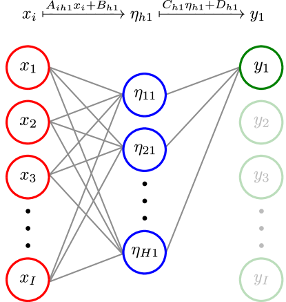
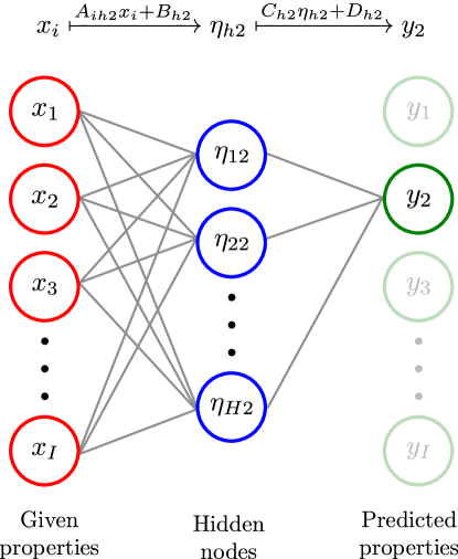
Figure 1: Artificial Neural Network (ANN) to interpolate data sets of materials properties. The graphs show how the outputs for $y_{1}$ (top) and $y_{2}$ (bottom) are computed from all the inputs $x_{i}$. $I-2$ similar graphs can be drawn for all other $y_{j}$ to compute all the predicted properties. Linear combinations (gray lines on the left) of the given properties (red) are taken by the hidden nodes (blue), a non-linear tanh operation is applied, and a linear combination (gray lines on the right) of those is returned as the predicted property (green).

We now define the framework that is used to capture the functional relation between all materials properties, and predict these relations for materials for which no information is available in the data set. The approach builds on the formalism used to design new nickel-base superalloys [9]. We intend to find a function $f$ that satisfies the fixed-point equation $\textbf{f}(\textbf{x})\equiv\textbf{x}$ as closely as possible for all elements x from the data set. There a total of $N$ entries in the data-set. Each entry $\textbf{x}=(x_{1},\ldots,x_{I})$ is a vector of size $I$, and holds information about $I$ distinct properties. The trivial solution to the fixed-point equation is the identity operator, so that $\textbf{f}(\textbf{x})=\textbf{x}$. However, this solution does not allow us to use the function $f$ to impute data, and so we seek a solution to the fixed-point equation that by construction is orthogonal to the identity operator. This will allow the function to predict a given component of x from some or all other components.

We choose a linear superposition of hyperbolic tangents to model the function f,

$$\textbf{f}:(x_{1},\ldots,x_{i},\ldots,x_{I})\mapsto(y_{1},\ldots,y_{j},\ldots,y_{I})$$ (1)

$$\begin{array}[]{lrl}\qquad\mathrm{with}&y_{j}&=\sum_{h=1}^{H}C_{hj}\eta_{hj}+D_{j},\\ \qquad\mathrm{and}&\eta_{hj}&=\tanh\left(\sum_{i=1}^{I}A_{ihj}x_{i}+B_{hj}\right)\,.\end{array}$$ (4)

This is an ANN with one layer of hidden nodes, and is illustrated in Fig. 1. Each hidden node $\eta_{hj}$ with $1\leq h\leq H$ and $1\leq j\leq I$ performs a $\tanh$ operation on a superposition of input properties $x_{i}$ with parameters $A_{ihj}$ and $B_{hj}$ for $1\leq i\leq I$. Each property is then predicted as a superposition of all the hidden nodes with parameters $C_{hj}$ and $D_{j}$. This is performed individually for each predicted property $y_{j}$ for $1\leq j\leq I$. There are exactly as many given properties as predicted properties, since all types of properties (defining and physical) are treated equally by the ANN. Provided a set of parameters $A_{ihj}$, $B_{hj}$, $C_{hj}$, and $D_{j}$, the predicted properties can be computed from the given properties. The ANN always sets $A_{khk}=0$ for all $1\leq k\leq I$ to ensure that the solution of the fixed-point equation is orthogonal to the identity, and so we derive a network that can predict $y_{k}$ without the knowledge of $x_{k}$.

2.2 Handling incomplete data

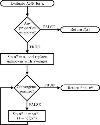
Figure 2: If we want to evaluate the ANN for a data point x which has some of the entries for its properties missing, we will follow the process described by this graph. After checking for the trivial case where all entries are existent, we set $\textbf{x}^{0}=\textbf{x}$, and replace all the missing entries by averages from the training data set. We then iteratively compute $\textbf{x}^{n+1}$ as a combination $\textbf{x}^{n}$ and f applied to $\textbf{x}^{n}$ until a certain point of convergence is reached, and return the final $\textbf{x}^{n}$ as a result instead of $\textbf{f}(\textbf{x})$.

Typically, materials data that has been obtained from experiments is incomplete, i.e. not all properties are known for every material, but the set of missing properties is different for each entry. However, there is information embedded within property-property relationships: for example ultimate tensile strength is three times hardness. A typical ANN formalism requires that each property is either an input or an output of the network, and all inputs must be provided to obtain a valid output. In our example composition would be inputs, whereas ultimate tensile strength and hardness are outputs. To exploit the known relationship between ultimate tensile strength and hardness, and allow either the hardness and ultimate tensile strength to inform missing data in the other property, we treat all properties as both inputs and outputs of the ANN. We have a single ANN rather than an exponentially large number of them (one for each combination of available composition and properties). We then adopt an expectation-maximization algorithm[17]. This is an iterative approach, where we first provide an estimate for the missing data, and then use the ANN to iteratively correct that initial value.

The algorithm is shown in Fig. 2. For any material x we check which properties are unknown. In the non-trivial case of missing entries, we first set missing values to the average of the values present in the data set. An alternative approach would be to adopt a value suggested by that of a local cluster. With estimates for all values of the neural network we then iteratively compute

$$\textbf{x}^{n+1}=\gamma\textbf{x}^{n}+(1-\gamma)\textbf{f}(\textbf{x}^{n})\,.$$ (5)

The converged result is then returned instead of $\textbf{f}\textbf{(}\textbf{x})$. The function f remains fixed on each iteration of the cycle.

We include a softening parameter $0\leq\gamma\leq 1$. With $\gamma=0$ we ignore the initial guess for the unknowns in x and determine them purely by applying f to those entries. However, introducing $\gamma>0$ will prevent oscillations and divergences of the sequence, typically we set $\gamma=0.5$.

2.3 Functional properties

Many material properties are functional graphs, for example to capture the variation of the yield stress with temperature[15]. To handle this data efficiently, we promote the two varying quantities to become interdependent vectors. This will reduce the amount of memory space and computation time used by a factor roughly proportional to the number of entries in the vector quantities. It also allows the tool to model functional properties on the same footing as the main model, rather than as a parameterization of the curve such as mean and gradient. The graph is represented by a series of points indexed by variable $\ell$. Let x be a point from a training data set. Let $x_{1,\ell}$ and $x_{2,\ell}$ be the varying graphical properties, and let all other properties $x_{3},x_{4},\ldots$ be normal scalar quantities. When $\textbf{f}(\textbf{x})$ is computed, the evaluation of the vector quantities is performed individually for each component of the vector,

$$y_{1,l}=f_{1}(x_{1,\ell},x_{2,\ell},x_{3},x_{4},\ldots)\,.$$ (6)

When evaluating the scalar quantities, we aim to provide the ANN with information of the $x_{2}(x_{1})$ dependency as a whole, instead of the individual data points (i.e. parts of the vectors $x_{1,\ell}$, and $x_{2,\ell}$). It is reasonable to describe the curve in terms of different moments with respect to some basis functions for modeling the curve. For most expansions, the moment that appears in lowest order is the average $\left\langle x_{1}\right\rangle$, or $\left\langle x_{2}\right\rangle$ respectively. We therefore evaluate the scalar quantities by computing,

$$y_{3}=f_{3}(\left\langle x_{1}\right\rangle,\left\langle x_{2}\right\rangle,x_{3},x_{4},\ldots)\,.$$ (7)

This can be extended by defining a function basis for expansion, and include their higher order moments. This approach automatically removes the bias due to differeing numbers of points in the graphs.

2.4 Training process

The ANN has to first be trained on a provided data set. Starting from random values for $A_{ihj}$, $B_{hj}$, $C_{hj}$, and $D_{j}$, the parameters are varied following a random walk, and the new values are accepted, if the new function f models the fixed-point equation $\textbf{f}(\textbf{x})=\textbf{x}$ better. This is quantitatively measured by the error function,

$$\delta=\sqrt{\frac{1}{N}\sum_{x\in X}\sum_{j=1}^{I}\left[f_{j}(\textbf{x})-x_{j}\right]^{2}}\,.$$ (8)

The optimization proceeds by a steepest descent approach[18], where the number of optimization cycles $C$ is a run-time variable.

In order to calculate the uncertainty in the ANN’s prediction, $\textbf{f}^{\sigma}(\textbf{x})$, we train a whole suite of ANNs simultaneously, and return their average as the overall prediction and their standard deviation as the uncertainty[19]. We choose the number of models $M$ to be between $4$ and $64$, since this should be sufficient to extract the mean and uncertainty. In Section 3 we show how the uncertainty reflects the noise in the training data and uncertainty in interpolation. Moreover, on systems that are not uniquely defined, knowledge of the full distribution of models will expose the degenerate solutions.

2.5 Alternative approaches

ANNs like the one proposed in this paper (with one hidden layer and a bounded transfer function; see Eq. (1)) can be expressed as a Gaussian process using the construction first outlined by Neal [20] in 1996. Gaussian processes were considered as an alternative to building the framework in this paper, but were rejected for two reasons. Firstly, the ANNs have a lower computational cost, which scales linearly with the number of entries $N$, and therefore ANNs are feasible to train and run on large-scale databases. The cost for Gaussian processes scales as $N^{3}$, and therefore does not provide the required speed. Secondly, materials data tends to be clustered. Often, experimental data is easy to produce in one region of the parameter space, and hard to produce in another region. Gaussian processes can only define a unique length-scale of correlation and consequently fail to model clustered data whereas ANNs perform well.

3 Testing and validation

Having developed the ANN formalism, we proceed by testing it on exemplar data. We will take data from a range of models to train the ANN, and validate its results. We validate the ability of the ANN to capture functional relations between materials properties, handle incomplete data, and calculate graphical quantities.

In Section 3.1, we interpolate a set of 1-dimensional functional dependencies (cosine, logarithmic, quadratic), and present a method to determine the optimal number of hidden nodes. In Section 3.2, we demonstrate how to determine erroneous entries in a data set, and to predict the number of remaining erroneous entries. Section 3.3 provides an example of the ANN performing on incomplete data sets. Finally, in Section 3.4, we present a test for the ANN’s graphing capability.

3.1 One-dimensional tests

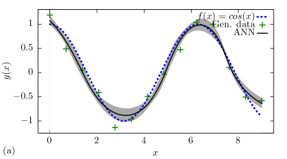
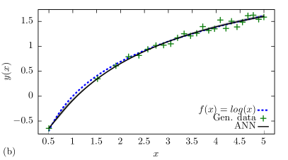
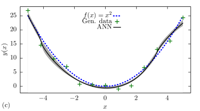
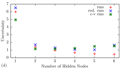
Figure 3: Training an ANN on toy-model data for (a) a cosine function, (b) a logarithmic function with unequally distributed data, and (c) a quadratic function with Gaussian noise. (d) For the quadratic function, the performance with different number of hidden nodes is tested, and the rms (Eq. (8)), the reduced rms (Eq. (9)), and the cross-validation rms are computed and plotted.

Table 1: The results of cross-validation testing for the three models (a) a cosine function, (b) a logarithmic function with unequally distributed data, and (c) a quadratic function with Gaussian noise. The second column gives the error when the ANN is trained on all of the data, and the third column the error in points unseen in training during cross-validation.

Data set	Error all	Error cross-validation
Cosine	$0.06$	$0.07$
Logarithm	$0.05$	$0.06$
Quadratic	$1.2$	$1.4$

The ANN was trained on a (a) cosine function, (b) logarithmic function with unequally distributed data, and (c) quadratic function with results shown in Fig. 3. All of the data is generated with Gaussian distributed noise to reflect experimental uncertainty in real-world material databases. The cosine function is selected to test the ability to model a function with multiple turning points, and was studied with $H=3$ hidden nodes. The logarithmic function is selected because it often occurs in physical examples such as precipitate growth, and is performed with $H=1$. The quadratic function is selected because it captures the two lowest term in a Taylor expansion, and is performed with $H=2$.

Fig. 3 shows that the ANN recovers the underlying functional dependence of the data sets well. The uncertainty of the model is larger at the boundaries, because the ANN has less information about the gradient. The uncertainty also reflects the Gaussian noise in the training data, as can be observed from the test with the $\log$ function, where we increased the Gaussian noise of the generated data from left to right in this test. For the test on the $\sin$ function, the ANN has a larger uncertainty for maxima and minima, because these have higher curvature, and are therefore harder to fit. The correct modeling of the smooth curvature of the cosine curve could not be captured by simple linear interpolation.

The choice of the number of hidden nodes $H$ is critical: Too few will prevent the ANN from modeling the data accurately; too many hidden nodes leads to over-fitting. To study the effect of changing the number of hidden nodes, we repeat the training process for the quadratic function with $1\leq H\leq 6$, and determine the error $\delta$ in three ways. Firstly, the straight error $\delta$. The second approach is cross-validation by comparing to additional unseen data[21]. The third and final approach is evaluate the reduced error

$$\delta^{*}=\frac{\delta}{\sqrt{1-2H/N}}\,,$$ (9)

which assumes that the sum of the squares in Eq. (8) is $\chi^{2}$-distributed, so we calculate the error per degree of freedom, which is $N-2H$, where the $2H$ parameters in the ANN arise because each of the $H$ indicator functions in Eq. (1) has two degrees of freedom: a scaling factor and also a shift. The results are presented in Fig. 3(d).

The error, $\delta$, monotonically falls with more hidden nodes. This is expected as more hidden nodes gives the model the flexibility to describe the training data more accurately. However, it is important that the ANN models the underlying functional dependence between those data points well, and does not introduce overfitting. The cross-validation results increase above $H=2$ hidden nodes, which implies that overfitting is induced beyond this point. Therefore, $H=2$ is the optimal number of hidden nodes for the quadratic test. This is expected since we choose $\tanh$ as the basis functions to build our ANN, which is a monotonic function, and the quadratic consists of two parts that are decreasing and increasing respectively.

In theory, performing a cross-validation test may provide more insight into the performance of the ANN on a given data set, however, this is usually not possible because it has a high computational cost. We therefore turn to the reduced error, $\delta^{*}$. This also has a minimum at $H=2$, and represents a quick and robust approach to determine the optimal number of hidden nodes.

Cross-validation also provides an approach to confirm the accuracy of the ANN predictions. For the optimal number of hidden nodes we perform a cross-validation analysis by taking the three examples in Fig. 3, remove one quarter of the points at random, train a model on the remaining three quarters of the points, and then re-predict the unseen points. We then compare the error to the predictions of an ANN trained on the entire data set. The results are summarized in Table 1. The error in the cross-validation analysis is only slightly larger than the error when trained off all entries, confirming the accuracy of the ANNs.

In this section, we were able to prove that the ANN is able to model data accurately, and laid out a clear prescription for determining the optimal number of hidden nodes by minimizing $\delta^{*}$.

3.2 Erroneous entries

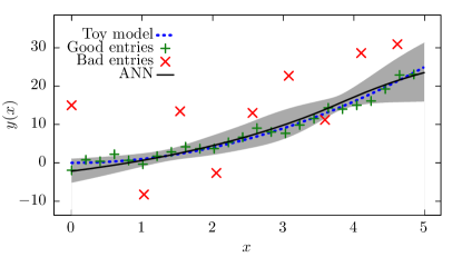
Figure 4: Blue dashed line: Quadratic curve for generating data. Red/green points: Data points generated from the blue line with Gaussian noise that have/have not been identified as erroneous. Black line: Prediction of the model with uncertainty. The Gaussian noise of the generated data increases proportional to the value of the toy-model function. Observe that less points are identified as erroneous at the right end of the plot, since the certainty of the ANN is lower in that region.

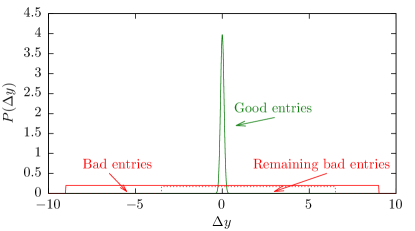
Figure 5: Theory of how many entries should be left using a uniform distribution of ’bad’ entries.

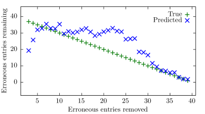
Figure 6: Blue points: the neural network prediction of, after removing a certain number of erroneous entries (x-axis), how many erroneous entries remain in the data set. A perfect prediction of the remaining number of erroneous entries would be the green points.

The ANN can be used to search for erroneous entries in a data set. As the ANN captures the functional dependence of the training data and the uncertainty in the estimate, the likelihood of an entry being erroneous can be determined by computing the number of standard deviations that this entry lies away from the ANN’s prediction,

$$\Delta_{\sigma}(\textbf{x})=\sum_{j=1}^{G}\frac{f_{j}(\textbf{x})-x_{j}}{f^{\sigma}_{j}(\textbf{x})}\,.$$ (10)

For a well-behaved data set with no errors the average absolute value of $\Delta_{\sigma}$ should be approximately unity. However, in the presence of erroneous entries, those entries with anomalously large $\Delta_{\sigma}(\textbf{x})$ can be identified, removed, or corrected. In this section, we will analyze the ability of the ANN to uncover erroneous entries in an exemplar set of data.

The case study is based on a quadratic function shown in Fig. 4 containing $N_{\textrm{g}}$ ‘good’ points and $N_{\textrm{b}}$ ‘bad’ points. Good points would be the experimental data with small Gaussian distributed noise, whereas bad points would occur through strong systematic mistakes modeled with a broad uniform distribution shown in Fig. 5. The results are shown in Fig. 4, where only $25\text{\,}\mathrm{\char 37\relax}$ of the data is plotted. The ten points that are identified to be the most erroneous ones in this set are removed first, and have been highlighted in the graph.

The upper limit of $\Delta_{\sigma}$ that we use to extract erroneous entries from the data set has to be chosen correctly. We want to eliminate as many erroneous entries as possible, while not removing any entries that hold useful information. We therefore proceed by developing a practical method to analyze how many erroneous data entries are expected to remain in the data set after extracting a certain number of entries. In a practical application, the maintainer of a large materials database might opt to continue removing erroneous entries from the database until the expected number of erroneous entries that a user would encounter falls below 1.

The probability density for finding erroneous entries in the region where erroneous entries have been removed from the sample is approximately equal to the probability density for finding further erroneous entries in the region of remaining entries. Therefore, the expected number of remaining erroneous entries is

$$N_{\textrm{rem}}=\frac{N_{\textrm{found}}}{1-\frac{\Delta y_{\textrm{rem}}}{\Delta y_{\textrm{tot}}}}\,,$$ (11)

where $N_{\textrm{rem,found}}$ are the number of remaining and found erroneous data entries respectively, and $\Delta y_{\textrm{tot,rem}}$ refer to the range over which the total and remaining entries are spread respectively.

Returning to the exemplar data set, we compare $N_{\textrm{rem}}$ with the true number of remaining erroneous entries in Fig. 6. The method provides a good prediction for the actual number of remaining erroneous entries.

The neural network can identify the erroneous entries in a data set. Furthermore, the tool can predict which are the entries most likely to be erroneous allowing the end user to prioritize their attention on the worse entries. The capability to predict the remaining number of entries allows the end user to search through and correct erroneous entries until a target quality threshold is attained.

3.3 Incomplete data

In the following section, we investigate the capability of the ANN to train on and analyze incomplete data. This requires at least three different properties to study, and therefore our tests will be on three-dimensional data sets. This procedure can be studied for different levels of correlation between the properties, and we study two limiting classes: completely uncorrelated, and completely correlated data. In the uncorrelated data set the two input variables are uncorrelated with each other, but still correlated to the output. In the correlated data set the input variables are now correlated with each other, and also correlated to the output. We focus first on the uncorrelated data.

3.3.1 Fully uncorrelated data

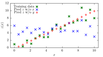
Figure 7: The toy-model data that is used for training of the ANN is shown as $Z$ as a function of $X$ together with the predictions of the ANN without providing $X$ or $Y$ respectively. The ANN learns the $Z=X+Y$ dependence, and uses the average of $X$ or $Y$ values respectively to replace the unknown values.

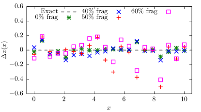
Figure 8: Deviation $\Delta z$ of the predicted values of $Z$ from the true values from the training data set as a function of $X$. An exact prediction would be represented by $\Delta z=0$ as indicated by the dashed gray line. The accuracy of the ANN predictions get worse with increasing level of fragmentation of the training data set.

To study the performance on uncorrelated data we perform the following two independent tests: we first train the ANN on incomplete uncorrelated data, and run it on complete data, and secondly train on complete uncorrelated data, and run on incomplete data.

For $N=20$ points $X=\{x_{1},\ldots,x_{N}\}$ distributed evenly in the interval $0\leq x\leq 10$ we generate a set of random numbers $Y=(y_{1},\ldots,y_{N})$ uniformly distributed between $-2.52.5$. We let $Z=X+Y=(x_{1}+y_{1},\ldots,x_{N}+z_{N})$, which is shown in Fig. 7. This data set is uncorrelated because the values of $Y$, a set of random numbers, are independent of the values $X$; therefore a model needs both $x$ and $y$ to calculate $z$.

We first train the ANN on all of the training data, and ask it to predict $z$ while providing (i) $x$ and $y$, (ii) $x$ only, and (iii) $y$ only. The results of (ii) and (iii) are shown in Fig. 8 alongside the training data, where $z$ is plotted as a function of $x$. Fig. 8 reveals that when provided with both $x$ and $y$ the ANN is able to capture the full $z=x+y$ dependence for the complete training data with maximum deviation $|\Delta z|\leq 0.13$. However, when the ANN is provided only with the $x$ values, but not $y$, the best that the ANN could do is replace $y$ with its average value, $0$. Fig. 7 confirms that the ANN returns $z=x+\left\langle Y\right\rangle=x$. However, when the ANN is provided with the $y$ values but not the $x$, the best that the ANN could do is replace $x$ with its average value, $5$. Fig. 7 shows that it returns $z=\left\langle X\right\rangle+y=5+y$. This confirms that after training off a complete uncorrelated data set, that when confronted with incomplete data, the ANN delivers the best possible predictions given the data available. The analysis also confirms the behavior of the ANN when presented with completely randomly distributed data: it correctly predicts the mean value as the expected outcome.

The second scenario is to train the ANN on an incomplete data set. Later, when using the neural network to predict values of $z$, values for both $x$ and $y$ are provided. We take the original training data, and randomly choose a set of entries (in any of $X$, $Y$, or $Z$), and set them as blank. We train the ANN on data sets that are (i) complete, (ii) $40\text{\,}\mathrm{\char 37\relax}$, (iii) $50\text{\,}\mathrm{\char 37\relax}$, and (iv) $60\text{\,}\mathrm{\char 37\relax}$ missing values. The ANN is then asked to predict $z$ for given $x$ and $y$, and the error in the predicted value of $z$ shown in Fig. 8. The accuracy of the ANN predictions decreases with increasing fragmentation of the training data. Yet, even with $60\text{\,}\mathrm{\char 37\relax}$ fragmentation the ANN is still able to capture the $z=x+y$ accurately with $\left|\Delta z\right|\leq 0.41$ $60\text{\,}\mathrm{\char 37\relax}$. This is less than the separation of $0.5$ between adjacent points in $Z$, so despite over half of the data missing the ANN is still able to distinguish between adjacent points.

3.3.2 Fully correlated data

We next turn to a data set in which given just one parameter, either $x$ or $y$, it is possible to recover $z=x+y$. This requires that $y$ is a function of $x$, and so is fully correlated. We now set $y=x^{2}$, and perform the tests as above. Now after training on a complete data set, the ANN is able to predict values for $z$ when given only $x$ or $y$. The ANN also performs well when trained from an incomplete data set.

3.3.3 Summary

We have successfully tested the capability of the ANN to handle incomplete data sets. We performed tests for both training and running the ANN with incomplete data. The ANN performs well when the training data is both fully correlated and completely uncorrelated, so should work well on real-life data.

3.4 Functional properties

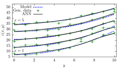
Figure 9: Training data, true function and predicted ANN function for different values of $x$.

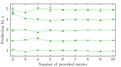
Figure 10: Predict $x$ from the training data with different number of $(y,z)$- pairs provided. The gray dotted lines indicate the true value of $x$.

We now test the capability for the ANN to handle data with functional properties (also referred to as graphing data) as a single entity. As before we have a functional variable $X=\{x_{1},\ldots,x_{N}\}$ with $N=5$ equidistant points in the interval from 1 to 5. At each value of $x$ point we introduce a vector quantity, dependent on a variable $Y=\{y_{1},\ldots,y_{\ell}\}$ that can have up to $\ell=10$. We compute the vector function $z_{\ell}=4x+y_{\ell}^{2}/4$, with additional Gaussian noise of width 1 and train an ANN on this data set. We show the training data as well as the ANN prediction for $z$ in Fig. 9, which confirms that the ANN is able to predict the underlying functional dependence correctly.

The real power of the graphing capability is to predict $x$ with different number of elements provided in the vector $(y,z)$. We show the predictions of the ANN in Fig. 10. With all 10 components of the vector provided the ANN makes accurate predictions for $x$. With fewer components provided the accuracy of the predictions for $x$ falls, but even if just 2 elements are provided the ANN is still able to distinguish between the discrete values of $x$.

We confirm that the ANN is able to fully handle vector and graphical data. The ANN gives accurate predictions for both the functional properties when providing non-functional properties only, and vice-versa. This new capability allows the ANN to handle a new form of real-world problems, for example the temperature dependence of variables such as yield stress. Temperature can be used only as an input for the yield stress, without the need to replicate other properties that are not temperature dependent, for example cost. The reduction in the amount of data required will increase the efficiency of the approach and therefore the quality of the predictions.

4 Applications

With the testing on model data complete we now present case studies of applying the ANN to real-life data. In this section, we will use the ANN framework to analyze the MaterialUniverse and Prospector Plastics databases. We first focus on a data set of 1641 metal alloys with a composition space of 31 dimensions (that is each metal is an alloy of potentially 31 chemical elements). We train neural networks of 4 hidden nodes to predict properties such as the density, the melting point temperature, the yield stress, and the fracture toughness of those materials. Secondly, we examine a system where not all compositional variables are available: a polymer data set of 5656 entries, and focus on the modeling of its tensile modulus.

We use the trained ANN to uncover errors by searching for entries multiple standard deviations $\Delta_{\sigma}$ away from the ANN predictions. We compare the results to primary sources referenced from the MaterialUniverse data set to determine whether the entry was actually erroneous: a difference could only be due to a transcription error from that primary data set into the MaterialUniverse database.

When analyzing the density data, we can confirm the ability of the ANN to identify erroneous entries with a fidelity of over $50\text{\,}\mathrm{\char 37\relax}$. For the melting temperature data, we show that for missing entries the ANN yields a significant improvement in the estimates provided by the curators of the database. When advancing to the yield stress properties of the materials, we observe that our methods can only be applied when additional heat treatment data is made available for training the ANN. Unlike established methods, our framework is uniquely positioned to include such data for error-finding and extrapolation. For the fracture toughness data, we exploit correlations with other known properties to provide more accurate estimation functions compared to established ones. Finally, in the polymer data, we exploit the capability of our ANN to handle an incomplete data set without compositional variables, and instead characterize polymers by their properties.

4.1 Density

Table 2: A list of MaterialUniverse entries (source) for density in $\mathrm{g}\text{\,}{\mathrm{cm}}^{-3}$ that were identified by the ANN as being potentially erroneous by the number of standard deviations $\Delta_{\sigma}$, and then subsequently confirmed to be incorrect by a primary source database (actual).

Alloy	Source	ANN	$\Delta_{\sigma}$	Actual
Stainless steel, Ilium P	$7.6$	$7.9$	$12$	$7.758.0$[4]
Tool steel, AISI M43	$8.4$	$8.0$	$-12$	$7.78.0$[4]
Copper-nickel, C70400	$8.5$	$8.9$	$11$	$8.9$[4]
Tool steel, AISI A3	$8.0$	$7.7$	$-20$	$8.9$[4]
Tool steel, AISI A4	$7.9$	$7.8$	$9$	$8.0$[4]
Tool steel, AISI M6	$8.5$	$8.0$	$11$	$7.78.0$[4]
Aluminum, 8091, T6	$2.6$	$2.5$	$10$	$2.5$[4]

The density of an alloy is set primarily by its composition, the data for which can be provided in a convenient form for training the ANN. This makes the density data set an attractive starting point for our investigation.

We first construct a model following the rule of mixtures by calibrating a weighted average of the densities of each constituent element to the MaterialUniverse density data. This model offers an average rms error of $0.19\text{\,}\mathrm{g}\text{\,}{\mathrm{cm}}^{-3}$. We then construct a data set that is the difference between the model and the original density data and compositions, and use this to train the ANN. The resulting rms error in the ANN prediction was $0.12\text{\,}\mathrm{g}\text{\,}{\mathrm{cm}}^{-3}$, a significant improvement on the rule of mixtures.

With an ANN model for density in place, we use it to search for erroneous entries within the density training set. For each entry we calculate the number of standard deviations from the ANN prediction, with the top 20 being considered as candidates for being erroneous. Of the 20 entries with highest $\Delta_{\sigma}$, 7 were found to be incorrect after comparing to a primary data source, these entries tabulated in Table 2. Of the remaining 13, 7 are found to be correct, and no source of primary data could be found for the remaining 6. The ANN detected errors with a fidelity of $50\text{\,}\mathrm{\char 37\relax}$. Following these amendments, using Eq. (11), we predict that the the number of remaining erroneous entries to be 17.

The ability to identify erroneous entries in a materials database, as well as the ability to assess the overall quality should be of interest to the curators of such databases. We therefore now use the ANN to search for errors in other quantities in the MaterialUniverse data set.

4.2 Melting temperature

Table 3: Erroneous entries for melting temperature in $\mathrm{K}$ from the MaterialUniverse database (source) alongside predictions from the ANN, that differ by $\Delta_{\sigma}$ standard deviations, subsequently confirmed to be incorrect by a primary source databases (actual).

Alloy	Source	ANN	$\Delta_{\sigma}$	Actual
Wrought iron	$1973$	$1760$	$-37$	$1808$[4]
Nickel, INCOLOY840	$1419$	$1661$	$8$	$17241784$[22]
Titanium, $\alpha$-$\beta$	$1593$	$1878$	$17$	$1866$[4]
Steel, AISI 1095	$1650$	$1699$	$13$	$1788$[23]

Table 4: Differences in the estimates of the melting temperature in $\mathrm{K}$ from the actual value for the 7 points where the established fitting function (EFF), and the ANN differ the most and primary source data is available.

Alloy	$\Delta_{\textrm{EFF}}$	$\Delta_{\textrm{ANN}}$
Steel Fe-9Ni-4Co-0.2C, quenched[24]	-94	9
Tool steel, AISI W5, water-hardened[24]	48	-19
Tool steel, AISI A4, air-hardened[24]	56	16
Tool steel, AISI A10, air-hardened[23]	59	-61
Tool steel, AISI L6, $650\text{\,}\mathrm{\SIUnitSymbolCelsius}$ tempered[24]	59	14
Tool steel, AISI L6, annealed[24]	59	14
Tool steel, AISI L6, $315\text{\,}\mathrm{\SIUnitSymbolCelsius}$ tempered[24]	59	14

The melting point of a material is a complex function of its composition so modeling it is a stern test for the ANN formalism. Furthermore, the melting temperature data set in the MaterialUniverse database has $80\text{\,}\mathrm{\char 37\relax}$ of its data taken from experiments with the remaining $20\text{\,}\mathrm{\char 37\relax}$ estimated from a fitting function by the database curators. This means that we have to handle data with underlying differing levels of accuracy.

We begin by training the ANN on only the experimental data. We seek to improve the quality of the data set by searching and correcting erroneous entries as was done for density. After identifying and correcting the 4 incorrect entries listed in Table 3, we estimate that there are still 5 erroneous entries in the data set. This leaves us with just $0.3\text{\,}\mathrm{\char 37\relax}$ of the database being erroneous, and hence with a high-quality data set of experimental measurements to study the accuracy of the MaterialUniverse fitting function.

We now wish to quantify the improvement in accuracy of the ANN model over the established MaterialUniverse fitting model for those entries for which no experimental data is available. We do so by analyzing the 30 entries where the ANN and the fitting function are most different. By referring to primary data sources we confirmed that the ANN predictions are closer to the true value than the fitting function’s prediction in 20 cases, further away in 4 cases, and no conclusion is possible in 4 cases due to a lack of primary data.

Sometimes there are two sources of primary data that are inconsistent. In these cases we can use the ANN to determine which source is correct. Assuming that out of several experimental results only one can be correct, we can decide which one it is by evaluating $\Delta_{\sigma}$ for each entry, and comparing the resulting difference in likelihood for each of the values being correct. For example, for the alloy AISI O1 Tool steel, the value from one source is $1694\text{\,}\mathrm{K}$, only $0.6$ standard deviations away from the ANN prediction of $1698\text{\,}\mathrm{K}$, whereas the value given by the other source, $1723\text{\,}\mathrm{K}$, is $4.5$ standard deviations away. The value of $1694\text{\,}\mathrm{K}$ $\exp{(-0.6^{2})}/\exp{(-4.5^{2})}\approx 10^{9}$-times more likely to be correct and we can therefore confidently adopt this value.

The ANN yields a clear improvement over the established fitting model. Having accurate modeling functions available for is crucial for operators of materials databases, and improvements over current modeling functions will greatly benefit usage of those databases in industrial applications.

4.3 Yield stress

Table 5: The effect of adding heat treatment into the training set on the average error in the ANN predictions of yield stress. Separate results for ferrous and non-ferrous alloys as well as the entire metals data set are shown. The error from the established fitting model used within MaterialsUniverse is also shown.

Data set	Error
Composition alone	$0.349$
Composition and elongation	$0.092$
Composition, elongation, and heat treatment	$0.052$
Established model	$0.072$

Table 6: Erroneous entries for yield stress in $\mathrm{MPa}$ from the MaterialUniverse database (source) alongside predictions from the ANN, that differ by $\Delta_{\sigma}$ standard deviations, subsequently confirmed to be incorrect by a primary source databases (actual).

Alloy	Source	ANN	$\Delta_{\sigma}$	Actual
Stainless steel, AISI 301L	$193$	$269$	$5$	$238$[23]
Stainless steel, AISI 301	$193$	$267$	$5$	$221$[23]
Aluminum, 1080, H18	$51$	$124$	$5$	$120$[23]
Aluminum, 5083, wrought	$117$	$191$	$14$	$300$,$190$[4, 23]
Aluminum, 5086, wrought	$110$	$172$	$11$	$269$,$131$[4, 23]
Aluminum, 5454, wrought	$102$	$149$	$14$	$124$[23]
Aluminum, 5456, wrought	$130$	$201$	$11$	$165$[23]
Nickel, INCONEL600	$223$	$278$	$10$	$\geq 550$[23]

We now study yield stress, a property of importance for many engineering applications, and therefore one that must be recorded with high accuracy in the MaterialUniverse database. Yield stress is strongly influenced by not only the composition but also the heat treatment routine. Initial attempts to use composition alone produces an inaccurate ANN with relative error of $0.349$ because alloys with similar or identical compositions had undergone a different heat treatment and so have quite different yield stress. To capture the consequences of the heat treatment routine additional information can be included in the training set. For example, the elongation depends on similar microscopic properties to yield stress, such as the bond strength between atoms and the ease of dislocation movement, and so has a weak inverse correlation with yield stress. Elongation was therefore included in the training set, and as summarized in Table 5 we observed a reduction in the average error to $0.092$ as a result.

To directly include information about the heat treatment a bit-wise representation for encoding information on the range of different heat treatments into input data readable by the ANN was devised. This was achieved by representing the heat-treatment routine of an alloy bit-wise, indicating whether or not the alloy had undergone the possible heat treatments: tempering, annealing, wrought, hot or cold worked, or cast. Table 5 shows that including this heat treatment data allows the ANN to model the data better than established modeling frameworks, with the average error reduced to $0.052$. This error can be compared with the standard polynomial fitting model previously used by MaterialUniverse, which has an error of $0.072$. This confirms the increased accuracy offered by the ANN.

With the ANN model established, we can then use it to search for erroneous entries within the MaterialUniverse database. Following the prescription developed in density and melting point, of the twenty alloys with the largest $\Delta_{\sigma}$ in the estimate of yield stress, eight were confirmed by comparison to primary sources to be erroneous, and are included in Table 6. The other twelve entries could not be checked against primary sources, resulting in an fidelity in catching errors that could be confirmed of $100\text{\,}\mathrm{\char 37\relax}$.

4.4 Fracture toughness

Table 7: Error in the ANN when different quantities are used in the training data set to fit fracture toughness.

Data set	Relative error
Composition alone	$0.144$
Composition & elongation	$0.113$
Composition & young modulus	$0.136$
Composition & yield stress	$0.132$
Composition & UTS	$0.134$
Composition, elongation & yield stress	$0.106$

Table 8: Relative error in the available models for fracture toughness, calculated over only the experimentally determined data.

Model	ANN	Steels	Nickel	Aluminium
Logarithmic error	$0.065$	$0.188$	$0.102$	$0.086$
Data points	$202$	$81$	$5$	$57$

Fracture toughness indicates how great a load a material containing a crack can withstand before brittle fracture occurs. Although it is an important quantity it has proven to be difficult to model from first principles. We therefore turn to our ANN. Fracture toughness depends on both the stress required to propagate a crack and the initial length of the crack. We can therefore identify the UTS and yield stress as likely correlated quantities. Additionally, elongation a measure of the material’s ability to deform plastically, is also relevant for crack propagation.

The model functions fitted by the curator of MaterialUniverse all use composition as an input so we follow their prescription. An efficient way to identify the properties most strongly correlated to fracture toughness is to train the ANN with each quantity in turn (in addition to the composition data), and then evaluate the deviation from the fracture toughness data. The properties for which the error is minimized are the most correlated. Table 7 shows that elongation is the property most strongly correlated to fracture toughness. Whilst yield stress, Young modulus, and UTS offer some reduction in the error, including these quantities to the training data will not lead to a significant improvement on the average error obtained from composition and elongation alone.

The MaterialUniverse fracture toughness data contains only around $200$ values that have been determined experimentally, with the remaining $1400$ values estimated by fitting functions. These are polynomial functions which take composition and elongation as input, and are fitted to either steels, nickel, or aluminum separately. We train the ANN over just the experimentally determined data, and compare the error in its predictions to those from the known fitting functions. Table 8 shows that the ANN is the most accurate, having a smaller error than the fitting function for all three alloy families. While the different fitting functions are ‘trained’ only on the subset of the data for which they are designed, the ANN is able to use information gathered from the entire data set to produce a better model over each individual subset. This is one of the key advantages of a ANN over traditional data modeling methods.

4.5 Polymers

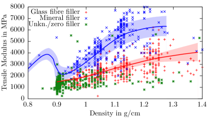
Figure 11: Polymer tensile modulus against density with glass fiber filler (blue) and mineral filler (red). The input information includes not only the filler type but also the filler amount (weight in %).

Table 9: A list of three ProspectorPlastics entries (source) for polymer flexural modulus/strength in $\mathrm{MPa}$ that were identified by the ANN as being potentially erroneous and then subsequently confirmed to be incorrect by a primary source databases (actual). The final five entries had missing filler type and amount in $\%$ that imputed by the ANN and then confirmed against a primary data source.

Polymer	Property	Source	ANN	Actual
4PROP25C21120	Modulus	$2\,300\,000$	$2186$	$2300$[25]
AZDELU400-B01N	Modulus	$8\,000\,000$	$8189$	$8000$[25]
Hyundai HT340	Strength	$469$	$46.1$	$46.9$[25]
Borealis NJ201AI	Mineral filler	-	$20\pm 4$	$20$[25]
Daplen EE168AIB	Mineral filler	-	$11\pm 3$	$10$[25]
Maxxam NM-818	Glass filler	-	$18\pm 4$	$20$[25]
FORMULA P 5220	Mineral filler	-	$19\pm 3$	$20$[25]
4PROP 9C13100	Mineral filler	-	$13\pm 3$	$10$[25]

In this section, we study polymers, which is an incomplete data set. Polymer composition cannot be described simply by percentage of constituent elements (as in the previous example with metals) due to the complexity of chemical bonding, so we must characterize the polymers by their properties. Some properties are physical, such as tensile modulus and density; others take discrete values, such as type of polymer or filler used, and filler percentage. As the data [6] was originally compiled from manufacturer’s data sheets, not all entries for these properties are known, rendering the data set incomplete.

We analyze a database of polymers that has the filler type as a class-separable property. Many other properties exhibit a split based on filler type, such as tensile modulus, flexural strength, or heat deflection temperature. We first focus on the tensile modulus shown in Fig. 11. Analysis of the predicted entries in Table 9 uncovers three erroneous entries that could be confirmed against primary source data. All three of these polymers had been entered into the database incorrectly, being either one or three orders of magnitude too large.

The data set is incomplete so many polymers have unknown filler type. The vast majority of entries sit at the expected density of $0.9\text{\,}\mathrm{g}\text{\,}{\mathrm{cm}}^{-3}$. However, some entries sit well away from there. Since the data set includes no other properties that can account for this discrepancy, a reasonable assumption is that these entries do not have zero filler, but instead are lacking filler information. The ANN applies this observation to predict the filler type and fraction. In Table 9 we show five polymers for which the filler type and fraction were correctly predicted when compared to primary sources of data.

Having successfully confirmed the ANN’s ability to model incomplete data, we have completed our tests on real-life data. The ANN can perform materials data analysis that has so far not been possible with established methods, and hence our framework yields an important improvement in operating large-scale materials databases. With polymers being another class of materials of great importance to industry, we have again shown how our approach will have an impact across a broad range industrial fields.

5 Conclusions

We developed an artificial intelligence algorithm and extended it to handle incomplete data, functional data, and to quantify the accuracy of data. We validated its performance for model data to confirm that the framework delivers the expected results in tests on the error-prediction, incomplete data, and graphing capabilities. Finally, we applied the framework to the real-life MaterialUniverse and Prospector Plastics databases, and were able to showcase the immense utility of the approach.

In particular, we were able to propose and verify erroneous entries, provide improvements in extrapolations to give estimates for unknowns, impute missing data on materials composition and fabrication, and also help the characterization of materials by identifying non-obvious descriptors across a broad range of different applications. Therefore, we were able to show how artificial intelligence algorithms can contribute significantly to innovation in researching, designing, and selecting materials for industrial applications.

The authors thank Bryce Conduit, Patrick Coulter, Richard Gibbens, Alfred Ireland, Victor Kouzmanov, Hauke Neitzel, Diego Oliveira Sánchez, and Howard Stone for useful discussions, and acknowledge the financial support of the EPSRC [EP/J017639/1] and the Royal Society. There is Open Access to this paper and data available at https://www.openaccess.cam.ac.uk.

References

- Ashby [2004] M. Ashby, Materials Selection in Mechanical Design, Butterworth-Heinemann, 2004.
- Jain et al. [2013] A. Jain, S. P. Ong, G. Hautier, W. Chen, W. D. Richards, S. Dacek, S. Cholia, D. Gunter, D. Skinner, G. Ceder, K. a. Persson, APL Materials 1 (2013) 011002. URL: http://link.aip.org/link/AMPADS/v1/i1/p011002/s1&Agg=doi. doi:10.1063/1.4812323.
- NoMaD [2017] NoMaD, http://nomad-repository.eu/, 2017.
- MatWeb, LLC [2017] MatWeb, LLC, http://www.matweb.com/, 2017.
- Granta Design [2017a] Granta Design, MaterialUniverse, CES EduPack 2017, https://www.grantadesign.com/products/data/materialuniverse.htm, 2017a.
- Granta Design [2017b] Granta Design, Prospector Plastics, CES EduPack 2017, https://www.grantadesign.com/products/data/ul.htm, 2017b.
- Zhang et al. [2008] S. Zhang, L. Li, A. Kumar, Materials Characterization Techniques, CRC, 2008.
- Tadmor and Miller [2011] E. Tadmor, R. Miller, Modeling Materials: Continuum, Atomistic and Multiscale Techniques, Cambridge University Press, 2011.
- Conduit et al. [2017] B. Conduit, N. Jones, H. Stone, G. Conduit, Materials & Design 131 (2017) 358.
- Conduit et al. [2014] B. Conduit, G. Conduit, H. Stone, M. Hardy, Development of a new nickel based superalloy for a combustor liner and other high temperature applications, Patent GB1408536, 2014.
- Conduit et al. [2013] B. Conduit, G. Conduit, H. Stone, M. Hardy, Molybdenum-niobium alloys for high temperature applications, Patent GB1307535.3, 2013.
- Conduit et al. [2014a] B. Conduit, G. Conduit, H. Stone, M. Hardy, Molybdenum-hafnium alloys for high temperature applications, Patent EP14161255, US 2014/223465, 2014a.
- Conduit et al. [2014b] B. Conduit, G. Conduit, H. Stone, M. Hardy, Molybdenum-niobium alloys for high temperature applications, Patent EP14161529, US 2014/224885, 2014b.
- Conduit et al. [2014c] B. Conduit, G. Conduit, H. Stone, M. Hardy, A nickel alloy, Patent EP14157622, amendment to US 2013/0052077 A2, 2014c.
- Ritchie and Knott [1973] R. Ritchie, J. Knott, J. Me. Phys. Solids 21 (1973) 395–410.
- Oliveira Jr. et al. [2016] O. Oliveira Jr., J. Rodrigues Jr., M. de Oliveira, Neural Networks (2016).
- Krishnan and McLachlan [2008] T. Krishnan, G. McLachlan, The EM Algorithm and Extensions, Wiley, 2008.
- Floudas and Pardalos [2008] C. Floudas, P. Pardalos, Encyclopedia of Optimization, Springer, 2008.
- Steck and Jaakkola [2003] H. Steck, T. Jaakkola, in: Advances in Neural Information Processing Systems 16: Proceedings of the 2003 Conference, p. 521.
- Neal [1996] R. Neal, Bayesian learning for neural networks, Lecture notes in statistics ; 118, Springer, New York, 1996.
- Hill and Lewicki [2005] T. Hill, P. Lewicki, Statistics: Methods and Applications, StatSoft, 2005.
- Longhai Special Steel Co., Ltd [2017] Longhai Special Steel Co., Ltd, China steel suppliers, http://www.steelgr.com/Steel-Grades/High-Alloy/incoloy-alloy-840.html, 2017.
- AZoM [2017] AZoM, https://www.azom.com/, 2017.
- Metal Suppliers Online, LLS [2017] Metal Suppliers Online, LLS, www.metalsuppliersonline.com/, 2017.
- PolyOne [2017] PolyOne, http://www.polyone.com/resources/technical-data-sheets/, 2017.