Minimizing the number of 5-cycles in graphs with given edge-density

Abstract

Motivated by the work of Razborov about the minimal density of triangles in graphs we study the minimal density of the 5-cycle $C_{5}$. We show that every graph of order $n$ and size $\left(1-\frac{1}{k}\right)\binom{n}{2}$, where $k\geqslant 3$ is an integer, contains at least

$$\left(\frac{1}{10}-\frac{1}{2k}+\frac{1}{k^{2}}-\frac{1}{k^{3}}+\frac{2}{5k^{4}}\right)n^{5}+o(n^{5})$$

copies of $C_{5}$. This bound is optimal, since a matching upper bound is given by the balanced complete $k$-partite graph. The proof is based on the flag algebras framework. We also provide a stability result. An SDP solver is not necessary to verify our proofs.

1 Introduction

It is believed that extremal graph theory was started by Turán [29] when he proved that any graph on $n$ vertices with more than $\frac{r-2}{2(r-1)}n^{2}$ edges must contain a copy of $K_{r}$ (i.e. a clique with $r$ vertices). The case $r=3$ was earlier proved by Mantel [17]. The general Turán problem is to determine the minimum number $\mathrm{ex}(n,H)$ of edges in an $n$ vertex graph that guarantees a copy of a graph $H$, and has been very widely studied. The Erdős–Stone Theorem [6] was a major breakthrough which asymptotically determined the value of $\mathrm{ex}(n,H)$ for all nonbipartite $H$. For such $H$ we have

$$\mathrm{ex}(n,H)=\frac{\chi(H)-2}{2(\chi(H)-1)}n^{2}+o(n^{2}).$$

The natural quantitative question that arises is how many copies of $H$ must be contained in a graph $G$ on $n$ vertices with $m>\mathrm{ex}(n,H)$ edges. This question has also been well studied. Obviously the number of edges $m$ can be expressed as a density parameter $p$ such that $m=p\binom{n}{2}$. Therefore, we will use the following notation. Let $G$ be a (large) graph of order $n$ and $H$ a small one. Define $\nu_{H}(G)$ to be the number of unlabeled copies (not necessary induced) of $H$ in $G$ and the corresponding density as

$$d_{H}(G)=\frac{\nu_{H}(G)}{|V(G)|^{|V(H)|}}.$$

Furthermore, for a given number $p\in[0,1]$ let

$$d_{H}(p)=\lim_{n\to\infty}\min_{G}d_{H}(G),$$

where the minimum is taken over all graphs $G$ of order $n$ and size $(p+o(1))\binom{n}{2}$. It is not hard to show by double-counting that the limit exists, see e.g. [23, Lemma 2.2].

When $H=K_{3}$ (that means it is a triangle) Moon and Moser [18] and also independently Nordhaus and Stewart [20] determined $d_{K_{3}}(p)$ for any $p=1-\frac{1}{k}$, where $k$ is a positive integer. We call such $p=1-\frac{1}{k}$ a Turán density. Some other partial results for the general $r$-clique $H=K_{r}$ were established by Lovász and Simonovits [14]. However, for arbitrary $p$ these problems remained open for over 50 years.

Then Razborov in his seminal paper [25] introduced the so-called flag algebras and, using them, determined $d_{K_{3}}(p)$ for any $p$ in [26]. Subsequently, Pikhurko and Razborov [22] characterized all almost extremal graphs. Very recently, Liu, Pikhurko and Staden [12] found the precise minimum number of triangles among graphs with a given number of edges in almost all range. Nikiforov [19] determined $d_{K_{4}}(p)$ for all $p$, and then Reiher [27] determined $d_{K_{r}}(p)$ for all $r$ and $p$.

In this paper we address the minimum density of the 5-cycle, $C_{5}$, in a graph with given edge density. We chose to investigate $C_{5}$ instead of $C_{4}$ since it is known due to Sidorenko [28] that for any fixed constant edge density $p$, the minimum $C_{4}$-density is achieved asymptotically by the random graph $G_{n,p}$. It is worth mentioning some other research related to 5-cycles. Specifically, Grzesik [8] and independently Hatami, Hladký, Král’, Norine and Razborov [9] proved that the maximum density of 5-cycles in a triangle-free graph that is large or its number of vertices is a power of 5 is achieved by the balanced blow-up of a 5-cycle. The extension to graphs of all sizes, with one exception on 8 vertices, was done by Lidický and Pfender [10]. This settled in the affirmative a conjecture of Erdős [5]. On the other hand, Balogh, Hu, Lidický, and Pfender [2] studied the problem of maximizing induced 5-cycles, and proved that this is achieved by the balanced iterated blow-up of a 5-cycle. This confirmed a special case of a conjecture of Pippinger and Golumbic [24].

The main result of this paper is as follows.

Theorem 1.

Let $k\geqslant 3$ be an integer. Define

$$p=1-\frac{1}{k}\quad\mbox{and}\quad\lambda=\frac{1}{10}-\frac{1}{2k}+\frac{1}{k^{2}}-\frac{1}{k^{3}}+\frac{2}{5k^{4}}.$$ (1)

Then

$$d_{C_{5}}(p)=\lambda.$$

We also have the following stability result. Let the Turán graph $T_{k}^{n}$ be the complete $k$-partite graph on $n$ vertices with part sizes as equal as possible.

Theorem 2.

For every integer $k\geqslant 3$ and real $\delta>0$ there is $\epsilon>0$ such that every graph $G$ with $n\geqslant 1/\epsilon$ vertices, at least $(p-\epsilon){n\choose 2}$ edges and at most $(\lambda+\epsilon)n^{5}$ copies of $C_{5}$ is within edit distance $\delta n^{2}$ from the Turán graph $T_{k}^{n}$, where $p$ and $\lambda$ are as in (1).

Observe that the above theorems (as stated) also hold in the case $k=2$ for which $d_{C_{5}}(\frac{1}{2})=0$. However, their validity in this case easily follows from known standard results. Although the proofs of Theorems 1 and 2 are based on the flag algebras framework, their verification does not require using any SDP solver.

Theorems 1 and 2 are proved in respectively Sections 2 and 3. Finally, in Section 4, we discuss the general edge density and provide an upper bound on $d_{C_{5}}(p)$ for any $p\in[0,1]$.

2 Proof of the main theorem

2.1 Upper bound

By considering the sequence of graphs $T_{k}^{n}$ as $n\to\infty$, we get

$$d_{C_{5}}(T_{k}^{n})=\frac{\left[\frac{1}{10}(k)_{5}+\frac{1}{2}(k)_{4}+\frac{1}{2}(k)_{3}\right]\left(\frac{n}{k}\right)^{5}}{n^{5}}+o(1),$$

where $(k)_{\ell}=k(k-1)\cdots(k-\ell+1)$ is the falling factorial. To justify the numerator, we count the number of $C_{5}$ copies with vertices in parts $V_{1},V_{2},V_{3},V_{4},V_{5}$ of the partition. These parts may not all be distinct: for example we may have $V_{1}=V_{3}$. However $T_{k}^{n}$ has no edges within these parts and so we know $V_{i}\neq V_{i+1}$. We count copies of $C_{5}$ by grouping them according to how many distinct parts there are among $V_{1},\ldots,V_{5}$. Now there are asymptotically $\frac{1}{10}(k)_{5}\left(\frac{n}{k}\right)^{5}$ copies that hit 5 different parts (label 5 distinct parts, choose one vertex in each part, and divide by 10 for overcounting). Also, there are asymptotically $\frac{1}{2}(k)_{4}\left(\frac{n}{k}\right)^{5}$ copies hitting 4 parts, and $\frac{1}{2}(k)_{3}\left(\frac{n}{k}\right)^{5}$ copies hitting 3 parts.

Simplifying, we get that $d_{C_{5}}(T_{k}^{n})=\lambda+o(1)$, which implies the upper bound in Theorem 1.

2.2 Lower bound

2.2.1 Preliminaries

The proof of the lower bound in Theorem 1 relies on the celebrated flag algebra method introduced by Razborov [25]. Here we briefly discuss the main idea behind this approach, referring the reader to [25] for all details. Alternatively, our lower bound is rephrased at the beginning of Section 3 by means of a combinatorial identity (namely (12)) whose statement does not use any flag algebra formalism.

Let $(G_{n})_{n\in\mathbb{N}}$ be a sequence of graphs, such that order of $G_{n}$ increases. Such a sequence is called convergent if for every fixed graph $H$, the density of $H$ in $G_{n}$ converges, i.e., for every $H$ there exists some number $\phi(H)$, such that

$$\lim_{n\to\infty}p(H,G_{n})=\phi(H),$$

where $p(H,G)$ is the probability that $|H|=|V(H)|$ vertices chosen uniformly at random from $V(G)$ induce a copy of $H$. (Here, it will be more convenient to count induced copies of $H$; see e.g. Equations (5.19)–(5.21) in [13] that show how to switch between induced and non-induced versions.) Notice that any sequence of graphs whose orders increase has a convergent subsequence. Thus, without loss of generality we assume $G_{n}$ is convergent. Note that $\phi$ cannot be an arbitrary function since it must satisfy many obvious identities such as $\phi(edge)+\phi(nonedge)=1$.

Interestingly, these $\phi$ exactly correspond to homomorphisms that we now describe. Denote by $\mathcal{F}$ the set of all graphs and by $\mathcal{F}_{\ell}$ the set of graphs of order $\ell$, up to an isomorphism. Let $\mathbb{R}\mathcal{F}$ be the set of all finite formal linear combinations of graphs in $\mathcal{F}$ with real coefficients. It comes with the natural operations of addition and multiplication by a real number. Let $\mathcal{K}$ be a linear subspace generated by all linear combinations

$$F-\sum_{H\in\mathcal{F}_{\ell}}p(F,H)\cdot H,$$ (2)

where $\ell>|F|$. Notice that $\phi$ evaluated at any element of $\mathcal{K}$ gives 0. Finally, let $\mathcal{A}$ be $\mathbb{R}\mathcal{F}$ factorized by $\mathcal{K}$. It is possible to define multiplication on $\mathcal{A}$, which we do in Section 2.2.3. It can be proved that $\mathcal{A}$ is indeed an algebra. Now limits of convergent graph sequences correspond to homomorphism $\phi$ from $\mathcal{A}$ to $\mathbb{R}$ such that $\phi(F)\geqslant 0$ for all $F\in\mathcal{F}$. Denote the set of all such homomorphisms by $Hom^{+}(\mathcal{A},\mathbb{R})$.

Let $OPT$ be the following linear combination, which counts the $C_{5}$ copies using induced subgraphs:

$$OPT=\vbox{\hbox{ \leavevmode\hbox to31.54pt{\vbox to31.54pt{\text{[drawing]}}}}}+\vbox{\hbox{ \leavevmode\hbox to31.54pt{\vbox to31.54pt{\text{[drawing]}}}}}+\vbox{\hbox{ \leavevmode\hbox to31.54pt{\vbox to31.54pt{\text{[drawing]}}}}}+2\vbox{\hbox{ \leavevmode\hbox to31.54pt{\vbox to31.54pt{\text{[drawing]}}}}}+2\vbox{\hbox{ \leavevmode\hbox to31.54pt{\vbox to31.54pt{\text{[drawing]}}}}}+4\vbox{\hbox{ \leavevmode\hbox to31.54pt{\vbox to31.54pt{\text{[drawing]}}}}}+6\vbox{\hbox{ \leavevmode\hbox to31.54pt{\vbox to31.54pt{\text{[drawing]}}}}}+12\vbox{\hbox{ \leavevmode\hbox to31.54pt{\vbox to31.54pt{\text{[drawing]}}}}},$$

where the coefficient of each graph is the number of copies of $C_{5}$ it contains. Thus,

$$\phi(OPT)=120\lim_{n\rightarrow\infty}d_{C_{5}}(G_{n}).$$ (3)

The factor $120=5!$ comes from the fact that $p(F,G_{n})$ for $F\in{\mathcal{F}}_{5}$ is the number of copies of $F$ divided by ${n\choose 5}$ whereas our scaling for $d_{C_{5}}$ was chosen as $n^{-5}$. Notice that $OPT$ can be written as a linear combination of all 34 graphs on 5-vertices, where 26 graphs have coefficient 0. Namely,

$$OPT=\sum_{F\in\mathcal{F}_{5}}c_{F}^{OPT}F,$$ (4)

where the nonzero entries $c_{F}^{OPT}$ are as above.

Our goal is to prove a good lower bound on

$$\min_{\phi\in Hom^{+}(\mathcal{A},\mathbb{R})}\phi(OPT),$$

given that that the edge density is $p$, that is, we have

$$\phi\left(\vbox{\hbox{ \leavevmode\hbox to24.93pt{\vbox to24.93pt{\text{[drawing]}}}}}\right)=p.$$ (5)

For this we find suitable $A\in\mathcal{A}$, such that $\phi(A)\geqslant 0$ for all $\phi\in Hom^{+}(\mathcal{A},\mathbb{R})$ with $\phi(K_{2})=p$, and use it in calculations. In particular, we will use it as $\phi(OPT)\geqslant\phi(OPT)-\phi(A)=\phi(OPT-A)\geqslant c$, where $c$ is the smallest coefficient $c_{F}$ when we express $OPT-A$ as $\sum_{F\in{\mathcal{F}}_{\ell}}c_{F}F$. Note that $A$ may contain both positive and negative coefficients, and these coefficients combine with coefficients in $OPT$.

When $p=1-\frac{1}{k}$ for integer $k\geqslant 3$, it is possible to prove the sharp lower bound as above by considering graphs of order 5 with only one labeled vertex. Similarly to defining the algebra $\mathcal{A}$ and limits of convergent graph sequences, one can define limits of sequences from the set $\mathcal{F}^{1}$ which consists of graphs with exactly one labeled vertex up a label-preserving isomorphism. This gives an algebra $\mathcal{A}^{1}$ and homomorphisms $Hom^{+}(\mathcal{A}^{1},\mathbb{R})$. In the following, we depict the labeled vertex by a square.

Let $X$ be the following column vector

$$X=(X_{1},\dots,X_{6})^{T}=\left(\vbox{\hbox{ \leavevmode\hbox to28.61pt{\vbox to28.61pt{\text{[drawing]}}}}},\vbox{\hbox{ \leavevmode\hbox to28.61pt{\vbox to28.61pt{\text{[drawing]}}}}},\vbox{\hbox{ \leavevmode\hbox to28.61pt{\vbox to28.61pt{\text{[drawing]}}}}},\vbox{\hbox{ \leavevmode\hbox to28.61pt{\vbox to28.61pt{\text{[drawing]}}}}},\vbox{\hbox{ \leavevmode\hbox to28.61pt{\vbox to28.61pt{\text{[drawing]}}}}},\vbox{\hbox{ \leavevmode\hbox to28.61pt{\vbox to28.61pt{\text{[drawing]}}}}}\right)^{T}.$$ (6)

Notice that $X$ is the vector of all graphs on 3 vertices with exactly one labeled vertex (the yellow square). For isomorphism, the labeled vertex must be preserved but the remaining two vertices may be swapped. If $M$ is a positive semidefinite matrix in $\mathbb{R}^{6\times 6}$, then for every $\phi^{1}\in Hom^{+}(\mathcal{A}^{1},\mathbb{R})$ it holds that

$$\phi^{1}\left(X^{T}MX\right)=\phi^{1}\left(X^{T}\right)M\phi^{1}\left(X\right)\geqslant 0,$$

where by $\phi^{1}\left(X\right)$ we mean the vector that results from applying $\phi^{1}$ to each coordinate of $X$.

Also, there is a linear operator $\left\llbracket\ \cdot\ \right\rrbracket_{1}:\mathbb{R}\mathcal{F}^{1}\to\mathbb{R}\mathcal{F}$ (which, roughly speaking, “unlabels” each $F\in\mathcal{F}^{1}$) such that for all $\phi\in Hom^{+}(\mathcal{A},\mathbb{R})$ we have $\phi\left(\llbracket X^{T}MX\rrbracket_{1}\right)\geqslant 0$. Furthermore, we have

$$\llbracket X^{T}MX\rrbracket_{1} =\sum_{F\in\mathcal{F}_{5}}c_{F}^{M}\cdot F,$$ (7)

see Section 2.2.3 for more details, in particular on how to calculate coefficients $c_{F}^{M}$.

Also, the relation (2) for cliques $K_{2}$ and $K_{1}$ gives that respectively $K_{2}=\sum_{H\in\mathcal{F}_{5}}p(K_{2},H)\cdot H$ and $1=K_{1}=\sum_{H\in\mathcal{F}_{5}}H$. Thus (5) can be written as an identity involving densities of $5$-vertex graphs.

Next, we take the sum of equations (4), (5) multiplied by some $\alpha$, and $\phi\left(\llbracket X^{T}MX\rrbracket_{1}\right)\geqslant 0$ expanded using (7), and obtain

$$\phi(OPT) \geqslant\phi(OPT)+\alpha\left(p-\phi\left(\vbox{\hbox{ \leavevmode\hbox to24.93pt{\vbox to24.93pt{\text{[drawing]}}}}}\right)\right)-\phi\left(\llbracket X^{T}MX\rrbracket_{1}\right)$$

$$=\phi\left(OPT+\alpha p-\alpha\vbox{\hbox{ \leavevmode\hbox to24.93pt{\vbox to24.93pt{\text{[drawing]}}}}}-\llbracket X^{T}MX\rrbracket_{1}\right)$$

$$=\phi\left(\sum_{F\in\mathcal{F}_{5}}\left(c_{F}^{OPT}+\alpha p-\alpha\cdot p(K_{2},F)-c_{F}^{M}\right)\cdot F\right)$$

(In Appendix A we provide $c_{F}^{OPT}$ and $p(K_{2},F)$ for each $F\in\mathcal{F}_{5}$.) For $F\in\mathcal{F}_{5}$, define

$$c_{F}=c_{F}^{OPT}+\alpha p-\alpha\cdot p(K_{2},F)-c_{F}^{M}.$$ (8)

With this notation

$$\phi(OPT)\geqslant\phi\left(\sum_{F\in\mathcal{F}_{5}}c_{F}\cdot F\right)\geqslant\min_{F\in\mathcal{F}_{5}}c_{F}\cdot\phi\left(\sum_{F\in\mathcal{F}_{5}}F\right)=\min_{F\in\mathcal{F}_{5}}c_{F},$$ (9)

where $c_{F}$ is a number that depends on the choice of $M$ and $\alpha$. Let us transfer this back to our extremal graph problem:

Lemma 3.

For every $p\in[0,1]$, $M\succcurlyeq 0$ and $\alpha\in{\mathbb{R}}$, with $c_{F}=c_{F}(p,M,\alpha)$ as in (8), we have

$$d_{C_{5}}(p)\geqslant\frac{1}{120}\min_{F\in\mathcal{F}_{5}}c_{F}.$$

Proof.

Suppose on the contrary we can find an increasing sequence of graphs $G_{n}$ with edge density $p+o(1)$ such that $d_{5}(G_{n})$ stays strictly below the stated bound. Take a convergent subsequence and let $\phi\in Hom^{*}({\mathcal{A}},{\mathbb{R}})$ be its limit. It satisfies (5) so the bound in (9) applies to $\phi$. However, this contradicts (3).∎

2.2.2 Finding the optimum

Let an integer $k\geqslant 3$ be fixed. Let $p$ and $\lambda$ be as in (1). By Lemma 3, in order to finish the proof of Theorem 1, it is enough to present some $M\succcurlyeq 0$ and $\alpha\in{\mathbb{R}}$ with $c_{F}\geqslant 5!\,\lambda$ for every $F\in\mathcal{F}_{5}$. Let

$$\alpha=\frac{1}{k^{3}}\left(60k^{3}-240k^{2}+360k-192\right).$$

In order to define the matrix $M$ we define first two matrices $A$ and $B$ as follows:

$$A=\begin{pmatrix}32k^{2}-96k+96&0&4k^{2}-16k\\ 0&10k^{4}-30k^{3}-8k^{2}+96k-96&-10k^{4}+35k^{3}-4k^{2}-80k+96\\ 4k^{2}-16k&-10k^{4}+35k^{3}-4k^{2}-80k+96&10k^{4}-40k^{3}+24k^{2}+64k-96\end{pmatrix}$$

and

$$B=\begin{pmatrix}k-1&1&k-2&0&k-3&-1\\ 0&2&k-2&0&2k-4&-2\\ 0&0&k-1&-1&2k-2&-2\end{pmatrix}.$$

It is easy to verify (by checking principal minors) that $A$ is positive definite for any $k\geqslant 3$. Therefore, the matrix

$$M=\frac{3}{2k^{4}}B^{T}AB$$ (10)

is positive semidefinite. In Section 2.2.4 we briefly describe how we determined matrices $A$ and $B$. With this choice of $M$ and $\alpha$, one can verify using for example Maple (see Appendix B) that coefficients $c_{F}$ satisfy:

$$c_{\scalebox{0.3}{ \leavevmode\hbox to31.54pt{\vbox to31.54pt{\text{[drawing]}}}}}=c_{\scalebox{0.3}{ \leavevmode\hbox to31.54pt{\vbox to31.54pt{\text{[drawing]}}}}}=c_{\scalebox{0.3}{ \leavevmode\hbox to31.54pt{\vbox to31.54pt{\text{[drawing]}}}}}=c_{\scalebox{0.3}{ \leavevmode\hbox to31.54pt{\vbox to31.54pt{\text{[drawing]}}}}}=c_{\scalebox{0.3}{ \leavevmode\hbox to31.54pt{\vbox to31.54pt{\text{[drawing]}}}}}=c_{\scalebox{0.3}{ \leavevmode\hbox to31.54pt{\vbox to31.54pt{\text{[drawing]}}}}}=c_{\scalebox{0.3}{ \leavevmode\hbox to31.54pt{\vbox to31.54pt{\text{[drawing]}}}}} =c_{\scalebox{0.3}{ \leavevmode\hbox to31.54pt{\vbox to31.54pt{\text{[drawing]}}}}}=c_{\scalebox{0.3}{ \leavevmode\hbox to31.54pt{\vbox to31.54pt{\text{[drawing]}}}}}=c_{\scalebox{0.3}{ \leavevmode\hbox to31.54pt{\vbox to31.54pt{\text{[drawing]}}}}}=c_{\scalebox{0.3}{ \leavevmode\hbox to31.54pt{\vbox to31.54pt{\text{[drawing]}}}}}=c_{\scalebox{0.3}{ \leavevmode\hbox to31.54pt{\vbox to31.54pt{\text{[drawing]}}}}}=$$

$$c_{\scalebox{0.3}{ \leavevmode\hbox to31.54pt{\vbox to31.54pt{\text{[drawing]}}}}}=c_{\scalebox{0.3}{ \leavevmode\hbox to31.54pt{\vbox to31.54pt{\text{[drawing]}}}}}=c_{\scalebox{0.3}{ \leavevmode\hbox to31.54pt{\vbox to31.54pt{\text{[drawing]}}}}}=c_{\scalebox{0.3}{ \leavevmode\hbox to31.54pt{\vbox to31.54pt{\text{[drawing]}}}}}=c_{\scalebox{0.3}{ \leavevmode\hbox to31.54pt{\vbox to31.54pt{\text{[drawing]}}}}}=c_{\scalebox{0.3}{ \leavevmode\hbox to31.54pt{\vbox to31.54pt{\text{[drawing]}}}}} =\frac{1}{5k^{4}}(60k^{4}-300k^{3}+600k^{2}-600k+240)$$

$$c_{\scalebox{0.3}{ \leavevmode\hbox to31.54pt{\vbox to31.54pt{\text{[drawing]}}}}}=c_{\scalebox{0.3}{ \leavevmode\hbox to31.54pt{\vbox to31.54pt{\text{[drawing]}}}}}=c_{\scalebox{0.3}{ \leavevmode\hbox to31.54pt{\vbox to31.54pt{\text{[drawing]}}}}}=c_{\scalebox{0.3}{ \leavevmode\hbox to31.54pt{\vbox to31.54pt{\text{[drawing]}}}}} =\frac{1}{5k^{4}}(66k^{4}-300k^{3}+600k^{2}-600k+240)$$

$$c_{\scalebox{0.3}{ \leavevmode\hbox to31.54pt{\vbox to31.54pt{\text{[drawing]}}}}} =\frac{1}{5k^{4}}(68k^{4}-300k^{3}+600k^{2}-600k+240)$$

$$c_{\scalebox{0.3}{ \leavevmode\hbox to31.54pt{\vbox to31.54pt{\text{[drawing]}}}}}=c_{\scalebox{0.3}{ \leavevmode\hbox to31.54pt{\vbox to31.54pt{\text{[drawing]}}}}}=c_{\scalebox{0.3}{ \leavevmode\hbox to31.54pt{\vbox to31.54pt{\text{[drawing]}}}}}=c_{\scalebox{0.3}{ \leavevmode\hbox to31.54pt{\vbox to31.54pt{\text{[drawing]}}}}} =\frac{1}{5k^{4}}(64k^{4}-300k^{3}+600k^{2}-600k+240)$$

$$c_{\scalebox{0.3}{ \leavevmode\hbox to31.54pt{\vbox to31.54pt{\text{[drawing]}}}}} =\frac{1}{5k^{4}}(65k^{4}-300k^{3}+600k^{2}-600k+240)$$

$$c_{\scalebox{0.3}{ \leavevmode\hbox to31.54pt{\vbox to31.54pt{\text{[drawing]}}}}}=c_{\scalebox{0.3}{ \leavevmode\hbox to31.54pt{\vbox to31.54pt{\text{[drawing]}}}}}=c_{\scalebox{0.3}{ \leavevmode\hbox to31.54pt{\vbox to31.54pt{\text{[drawing]}}}}}=c_{\scalebox{0.3}{ \leavevmode\hbox to31.54pt{\vbox to31.54pt{\text{[drawing]}}}}} =\frac{1}{5k^{4}}(62k^{4}-300k^{3}+600k^{2}-600k+240)$$

$$c_{\scalebox{0.3}{ \leavevmode\hbox to31.54pt{\vbox to31.54pt{\text{[drawing]}}}}}=c_{\scalebox{0.3}{ \leavevmode\hbox to31.54pt{\vbox to31.54pt{\text{[drawing]}}}}} =\frac{1}{5k^{4}}(61k^{4}-300k^{3}+600k^{2}-600k+240).$$

Since the entries only ever disagree in the $k^{4}$ coefficient, it is easy to see that the smallest $c_{F}$’s are in the first two rows and are equal to $5!\,\lambda$, as desired. (Recall that this proves the lower bound on $d_{C_{5}}(p)$ of Theorem 1 by Lemma 3.)

2.2.3 Products of graphs and determining $c_{F}^{M}$ coefficients

First, we define the product of unlabeled graphs. Recall that for a graph $G$ we denote $|V(G)|$ by $|G|$. Let $F_{1},F_{2},F$ in $\mathcal{F}$ be such that $|F_{1}|+|F_{2}|\leqslant|F|$. Choose uniformly at random two disjoint subsets $X_{1}$ and $X_{2}$ of $V(F)$ of sizes $|F_{1}|$ and $|F_{2}|$, respectively. Denote by $p(F_{1},F_{2};F)$ the probability that $F[X_{1}]$ is isomorphic to $F_{1}$ and $F[X_{2}]$ is isomorphic to $F_{2}$. Finally, the product of $F_{1}$ and $F_{2}$ is defined as

$$F_{1}\times F_{2}=\sum_{F\in\mathcal{F}_{|F_{1}|+|F_{2}|}}p(F_{1},F_{2};F)\cdot F.$$

The product can be extended to linear combinations of graphs and gives a multiplication operation in $\mathcal{A}$.

The product in $\mathcal{A}^{1}$ is defined along the same lines as in $\mathcal{A}$ but the intersection of $X_{1}$ and $X_{2}$ is exactly the labeled vertex. A more precise definition follows. Let $F_{1},F_{2},F$ in $\mathcal{F}^{1}$ such that $|F_{1}|+|F_{2}|\leqslant|F|-1$. Choose uniformly at random subsets $X_{1}$ and $X_{2}$ of $V(F)$ of sizes $|F_{1}|$ and $|F_{2}|$, respectively whose intersection is exactly the one labeled vertex. Denote by $p(F_{1},F_{2};F)$ the probability that $F[X_{1}]$ is isomorphic to $F_{1}$ and $F[X_{2}]$ is isomorphic to $F_{2}$, where isomorphism preserves the labeled vertex. Finally, the product of $F_{1}$ and $F_{2}$ is defined as

$$F_{1}\times F_{2}=\sum_{F\in\mathcal{F}_{|F_{1}|+|F_{2}|-1}}p(F_{1},F_{2};F)\cdot F.$$

Next we define the unlabeling operator $\left\llbracket\ \cdot\ \right\rrbracket_{1}:\mathcal{F}^{1}\to\mathbb{R}\mathcal{F}$. We extend $\left\llbracket\ \cdot\ \right\rrbracket_{1}$ to a linear function $\mathbb{R}\mathcal{F}^{1}\to\mathbb{R}\mathcal{F}$ which we also call $\left\llbracket\ \cdot\ \right\rrbracket_{1}$. Let $F\in\mathcal{F}^{1}$. Denote by $G\in\mathcal{F}$ the graph obtained from $F$ by unlabeling the labeled vertex. Let $v$ be a vertex in $G$ chosen uniformly at random. Let $q$ be the probability that $G$ with labeled $v$ is isomorphic to $F$. Then

$$\left\llbracket F\right\rrbracket_{1}=q\cdot G.$$

Recall that $X$ is the vector of all 3-vertex labeled graphs from ${\mathcal{F}}^{1}$:

$$X=(X_{1},X_{2},X_{3},X_{4},X_{5},X_{6})^{T}=\left(\vbox{\hbox{ \leavevmode\hbox to28.61pt{\vbox to28.61pt{\text{[drawing]}}}}},\vbox{\hbox{ \leavevmode\hbox to28.61pt{\vbox to28.61pt{\text{[drawing]}}}}},\vbox{\hbox{ \leavevmode\hbox to28.61pt{\vbox to28.61pt{\text{[drawing]}}}}},\vbox{\hbox{ \leavevmode\hbox to28.61pt{\vbox to28.61pt{\text{[drawing]}}}}},\vbox{\hbox{ \leavevmode\hbox to28.61pt{\vbox to28.61pt{\text{[drawing]}}}}},\vbox{\hbox{ \leavevmode\hbox to28.61pt{\vbox to28.61pt{\text{[drawing]}}}}}\right)^{T}.$$

In Appendix A we list all coefficients for products in $\mathcal{F}^{1}_{3}$, after unlabeling and multiplying by a scaling factor of 30 to clear denominators. Then we obtain that

$$\llbracket X^{T}MX\rrbracket_{1}=\sum_{i=1}^{6}\sum_{j=1}^{6}M_{i,j}\llbracket X_{i}\times X_{j}\rrbracket_{1}=\sum_{F\in\mathcal{F}_{5}}c_{F}^{M}\cdot F,$$

since each $\llbracket X_{i}\times X_{j}\rrbracket_{1}$ is a linear combination of graphs in $\mathcal{F}_{5}$.

2.2.4 Guessing matrices $A$ and $B$

In this paragraph we describe how we obtained the matrices $A$ and $B$. First, we used semidefinite programming to find a matrix $M$ for several small odd values of $k$. Notice that if (9) is applied to the extremal construction, then the left-hand side is equal to the right-hand side. That means that all inequalities used are actually equalities. In particular, $\phi\left(\llbracket X^{T}MX\rrbracket_{1}\right)=0$. Since $M$ is a positive semidefinite matrix, $X$ evaluated on our extremal example (the limit of $T_{k}^{n}$ as $n\to\infty$) must give an eigenvector of $M$ corresponding to the eigenvalue 0. The matrix $B$ was obtained by projecting onto the space orthogonal to three zero eigenvectors of $M$. As noted before, we had one zero eigenvector to start with. By looking at all eigenvectors of $M$, we managed to guess another zero eigenvector. We tried projection with the two zero eigenvectors and found the third one in the projection. After having obtained matrices $B$, we observed that a suitable $A$ exists even if we set the coordinate $[1,2]$ and $[2,1]$ to 0. With proper scaling of the objective function, we were getting nice matrices from the CSDP [3] solver with all entries integers. By using the solutions for several values of $k$, we calculated a polynomial function of $k$ fitting each entry in matrix $A$. Finally we observed that the same matrices $A$ and $B$ also work for even values of $k$.

3 Stability

In this section we prove Theorem 2. For this purpose it will be convenient to rewrite our lower bound as an asymptotic identity valid for an arbitrary graph. Fix $k\geqslant 3$. Let $p$ and $\lambda$ be as in (1). Let the matrix $M\succcurlyeq 0$, $\alpha\in{\mathbb{R}}$, and the reals $c_{F}^{M},c_{F}^{OPT},c_{F}$, indexed by $F\in{\mathcal{F}}_{5}$, be as previously.

Recall that $X=(X_{1},\dots,X_{6})^{T}$ is the vector of $3$-vertex rooted graphs defined in (6). For a graph $G=(V,E)$ of order $n\geqslant 5$ and a vertex $r\in V$, let $Y_{r}$ be the column vector whose $i$-th component is the number of unordered 2-sets $\{u,v\}\subseteq V\setminus\{r\}$ such that the induced graph $G[\{r,u,v\}]$ rooted at $r$ is isomorphic to $X_{i}$. Define $\overline{Y}=\frac{4}{5!}\,\sum_{r\in V}Y_{r}^{T}MY_{r}\geqslant 0.$

Let us argue that

$$\overline{Y}=\sum_{F\in{\mathcal{F}}_{5}}c_{F}^{M}P(F,G)+O(n^{4}),$$ (11)

where for $F\in{\mathcal{F}}_{\ell}$ we let $P(F,G)={n\choose\ell}p(F,G)$ be the number of $\ell$-sets inducing a copy of $F$ in $G$. Indeed, the $i$-th entry of $Y_{r}$ can be written as a double sum $\frac{1}{2}\sum_{u\in V}\sum_{v\in V}$ of the indicator function that $r,u,v$ are distinct and the graph $G[\{r,u,v\}]$ when rooted at $r$ is isomorphic to $X_{i}$. Using this representation of $Y_{r}$ and expanding everything, we can write $\overline{Y}$ as a sum over all $(r,u,v,u^{\prime},v^{\prime})\in V^{5}$ of some function that depends only on the graph induced by the (multi)set $(r,u,v,u^{\prime},v^{\prime})$ inside $G$. Apart of $O(n^{4})$ terms when some of the vertices coincide, the remaining ones can be grouped by the isomorphism type $F\in{\mathcal{F}}_{5}$ of $G[\{r,u,v,u^{\prime},v^{\prime}\}]$. For $F\in{\mathcal{F}}_{5}$, each unordered $5$-set spanning an induced copy of $F$ in $G$ contributes the same amount (depending only on $F$ and $M$) and the coefficient $c_{F}^{M}$ was in fact defined by us to be equal to this common value. Thus (11) holds.

Likewise, $P(K_{2},G){n-2\choose 3}$ and ${n\choose 5}$ can be written as fixed linear combinations of $P(F,G)$ over $F\in{\mathcal{F}}_{5}$. Also, $d_{C_{5}}(G)n^{5}=\sum_{F\in{\mathcal{F}}_{5}}c_{F}^{OPT}P(F,G)$ is the number of $5$-cycles in $G$. Putting all together, we obtain the following identity valid for an arbitrary graph $G$:

$$d_{C_{5}}(G)\,n^{5}+\frac{\alpha}{5!}\left(2P(K_{2},G)n^{3}-pn^{5}\right)-\overline{Y}+O(n^{4})=\sum_{F\in{\mathcal{F}}_{5}}c_{F}P(F,G),$$ (12)

where $c_{F}$ for $F\in{\mathcal{F}}_{5}$ was defined to be exactly the contribution of each induced copy of $F$ in $G$ to the left-hand side while all combinations when some vertices in the underlying 5-fold sum coincide are absorbed into the error term $O(n^{4})$.

Note that if we multiply (12) by ${n\choose 5}^{-1}$ then the scaled terms in (12) will be asymptotically the same as in (9) when $n\to\infty$. Since $\sum_{F\in{\mathcal{F}}_{5}}P(F,G)={n\choose 5}$, the right-hand size of (12) can be lower bounded by ${n\choose 5}\min_{F\in{\mathcal{F}}_{5}}c_{F}$, giving the required lower bound in Theorem 1 since each $c_{F}$ is at least $5!\,\lambda$.

Let us turn to stability. Take any sequence of graphs $G_{m}$ of strictly increasing orders such that

$$|E(G_{m})|\geqslant\left(p-\frac{1}{m}\right){|G_{m}|\choose 2}\quad\mbox{and}\quad d_{C_{5}}(G_{m})\leqslant\lambda+\frac{1}{m},\qquad\mbox{for all }m\in{\mathbb{N}}.$$ (13)

Observe that if $c_{F}>\lambda$ for some $F\in{\mathcal{F}}_{5}$, then the right-hand side of (12) is at least $(\lambda+(c_{F}-\lambda)p(F,G)){n\choose 5}.$ Thus we have that $p(F,G_{m})=o(1)$ as $m\to\infty$ for every such $F$. By looking at the explicit formulas for $c_{F}$ near the end of Section 2.2.2, we see that there are 16 such graphs. They are collected into the list $\mathcal{L}$ in Figure 1, and are denoted by $L_{1},\dots,L_{16}$ in this order.

Figure 1: The list $\mathcal{L}=(L_{1},\dots,L_{16})$

Let the co-cherry $\overline{P_{2}}$ be the complement of the 2-edge path $P_{2}$, that is, $\overline{P_{2}}$ is the graph with 3 vertices and 1 edge. Next, we show that its density in $G_{m}$ must also be $o(1)$. Note that there are 5-vertex graphs not in the list ${\mathcal{L}}$ that contain the co-cherry. Thus the naive approach does not work and a slightly more involved argument is needed.

Lemma 4.

For every sequence of graphs $G_{m}$ as in (13), we have that

$$\lim_{m\to\infty}p(\overline{P_{2}},G_{m})=0.$$

Proof.

Let $m$ be sufficiently large, $G=G_{m}$, $V=V(G)$ and $n=|V|$. For $i\in\{0,1,2\}$, let $F_{i}$ be the (unique) graph of order 4 with $i$ disjoint edges. Let ${\mathcal{L}}^{\prime}={\mathcal{L}}\cup\{F_{0},F_{1},F_{2}\}$.

Apply the induced removal lemma (see, e.g., [1, 4]) to $G$ to destroy all induced graphs in ${\mathcal{L}}^{\prime}$ whose density is $o(1)$. Formally, let $f=n^{-1}+\max\{p(L,G_{m}):L\in{\mathcal{L}}\}$ (and let initially $G=G_{m}$). As long as there is at least one $F\in{\mathcal{L}}^{\prime}$ with $0<p(F,G)\leqslant f$, change as few as possible adjacencies in $G$ to destroy all copies of all such $F$ so that, additionally, no graph in ${\mathcal{L}}^{\prime}$ absent from $G$ is introduced. Since $f$ tends to $0$ as $m\to\infty$ and the above iteration is applied at most $|{\mathcal{L}}^{\prime}|$ times (in fact, at most $|{\mathcal{L}}^{\prime}\setminus{\mathcal{L}}|+1=4$ times), we change $o(n^{2})$ edges in total by the induced removal lemma. Also, the final graph $G$ contains no graph from the list ${\mathcal{L}}$ since the first iteration destroyed all such subgraphs by our choice of $f$.

Claim 4.1.

$G$ contains no induced $F_{1}$ (i.e., 4 vertices spanning exactly one edge).

Proof.

Take a copy of $F_{1}$ and add one new vertex $x$ of degree $d$. If $d\in\{0,1,2,3\}$, then the sets of possible obtained graphs up to isomorphism are respectively $\{L_{1}\}$, $\{L_{2},L_{5}\}$, $\{L_{4},L_{6},L_{8}\}$, and $\{L_{7},L_{9}\}$. We see that each 1-vertex extension of $F_{1}$ is in ${\mathcal{L}}$ except when $d=4$ (that is, when $x$ is adjacent to every vertex of $F_{1}$). This means that for every copy of $F_{1}$, say on $A\subseteq V$, the set $A$ is complete to $V\setminus A$ in $G$. It follows that every two distinct induced copies of $F_{1}$ are vertex-disjoint and thus $G$ has at most $n/4$ such copies. This is at most $f{n\choose 4}$, so $G$ has no copy of $F_{1}$ at all.∎

Claim 4.2.

$G$ contains no induced $F_{2}$ (which is the matching with two edges).

Proof.

If we extend a copy of $F_{2}$ by adding a vertex $x$ of degree $d\in\{0,1,2,3\}$, then we obtain graphs in respectively $\{L_{5}\}$, $\{L_{8}\}$, $\{L_{11},L_{14}\}$ and $\{L_{15}\}$. Thus the only extension that does not lead to a graph in ${\mathcal{L}}$ is to connect $x$ to every vertex of $F_{2}$. This gives that every two distinct induced copies of $F_{2}$ in $G$ are vertex-disjoint. Thus we have at most $O(n)\leqslant f{n\choose 4}$ copies of $F_{2}$, that is, none at all.∎

Consider the edgeless 4-vertex graph $F_{0}$. If we add a vertex $x$ of degree $d\in\{1,2,3\}$, then we get respectively $L_{1}$, $L_{2}$ and $L_{3}$. The only remaining ways are to have $x$ empty or complete to $F_{0}$. Now, consider any copy of $F_{0}$ in $G$, say with vertex set $A_{0}\subseteq V(G)$. By above, every vertex outside of $A_{0}$ is empty or complete to $A_{0}$. Let $A\supseteq A_{0}$ consist of all vertices of $G$ that send no edges to $A_{0}$. Note that $A$ is an independent set: if we had an edge $xy$ inside $A$ then $x$, $y$ plus some two extra vertices from $A_{0}$ would span a copy of $F_{1}$ in $G$, contradicting Claim 4.1. Moreover, $A$ is complete to $V\setminus A$. Indeed, for every pair $(a,b)\in A\times(V\setminus A)$, the subgraph of $G$ induced by $a$ and some further three vertices of $A_{0}$ has no edges; thus the vertex $b\not\in A$ must be complete to it.

It follows that we can find disjoint independent sets $A_{i}$, $i\in I$, in $V$ such that each $A_{i}$ is complete to $V\setminus A_{i}$ while every copy of $F_{0}$ in $G$ is inside one of these sets $A_{i}$. Define $B=V\setminus(\cup_{i\in I}A_{i})$.

By the definition of $B$ and the above claims, we have that $H=G[B]$ is $\{F_{0},F_{1},F_{2}\}$-free. This means that the complement $\overline{H}$ of $H$ cannot have a (not necessarily induced) 4-cycle $C_{4}$ because for any way of filling its diagonals we get $F_{0}$, $F_{1}$ or $F_{2}$ in $H$. Thus $|E(\overline{H})|$ is at most the Turán function $\operatorname{ex}(n,C_{4})=O(n^{3/2})$, that is, $H$ is $O(n^{3/2})$-close in the edit distance to being a complete graph. We see that $G$ is $O(n^{3/2})$-close to the complete partite graph $G^{\prime}$ with parts $A_{i}$, $i\in I$, and $\{x\}$, $x\in B$. As every co-cherry in $G$ has to contain at least one pair where $E(G)$ and $E(G^{\prime})$ differ, $G$ has at most $O(n^{5/2})$ co-cherries.

Since the original graph $G_{m}$ and $G$ differ in $o(n^{2})$ adjacencies, the co-cherry density in $G_{m}$ is $o(1)$, as required.∎

Thus, another application of the induced removal lemma gives that we can change $o(1)$-fraction of adjacencies in $G_{m}$ and make it $\overline{P_{2}}$-free, that is, complete partite. Thus, in order to finish the proof of Theorem 2, it is enough to argue that each of the $k$ largest parts of $G_{m}$ has $(\frac{1}{k}+o(1))|G_{m}|$ vertices. We present two proofs of this. The first proof is more direct but longer. The second one is shorter but assumes some known facts about graphons.

3.1 First proof

We need the following auxiliary result.

Lemma 5.

Suppose a graph $J$ on $n$ vertices has a subgraph $X$ such that

1. $X$ has $x$ vertices where $\epsilon^{\prime}n\leqslant x\leqslant(1-\epsilon^{\prime})n$ and edge density $q\leqslant\frac{1}{2}$

2. $X$ is complete to $V(J)\setminus X$

3. $X$ contains at least $\frac{1}{2}x^{4}q^{3}+\epsilon^{\prime}x^{4}$ copies of $P_{4}$.

Then there exists a graph $J^{\prime}$ on $n$ vertices with asymptotically the same edge density as $J$ and

$$d_{C_{5}}(J^{\prime})\leqslant d_{C_{5}}(J)-\frac{1}{2}(\epsilon^{\prime})^{6}.$$

Proof.

Note first that conditions (i) and (ii) imply that $J$ is dense since it has at least $\epsilon^{\prime}(1-\epsilon^{\prime})n^{2}$ edges. We make $J^{\prime}$ by replacing $X$ with a $X^{\prime}$, which is a random balanced bipartite graph with edge probability $2q$. We will not change the rest of the graph, so $J^{\prime}-X^{\prime}=J-X$. W.h.p. $X^{\prime}$ has edge density asymptotically $q$ and so $J^{\prime}$ has asymptotically the same edge density as $J$. We will argue that $J^{\prime}$ has much fewer copies of $C_{5}$ than $J$ has, by considering several possible types of $C_{5}$ copies.

We will compare the copies according to how they intersect $X$ (for counting copies of $C_{5}$ in the graph $J$) or $X^{\prime}$ (in $J^{\prime}$). Specifically, since $X$ is complete to the rest of $J$ we have

$$\nu_{C_{5}}(J)=\sum_{H}m_{H}\nu_{H}(X)\cdot\nu_{C_{5}-H}(J-X)$$

where the sum is over all induced subgraphs $H\subseteq C_{5}$, and the coefficient $m_{H}$ is the number of $C_{5}$ copies contained in the graph formed by taking a copy of $H$ and a copy of $C_{5}-H$ with every possible edge in between. Recall that $\nu_{H}(G)$ counts the number of (not necessarily induced) copies of $H$ in $G$. Similarly, we have

$$\nu_{C_{5}}(J^{\prime})=\sum_{H}m_{H}\nu_{H}(X^{\prime})\cdot\nu_{C_{5}-H}(J^{\prime}-X^{\prime})=\sum_{H}m_{H}\nu_{H}(X^{\prime})\cdot\nu_{C_{5}-H}(J-X),$$

since $J^{\prime}-X^{\prime}=J-X$. So we will compare $\nu_{H}(X)$ with $\nu_{H}(X^{\prime})$ for each $H$. Specifically we will show that $\nu_{H}(X^{\prime})\leqslant(1+o(1))\nu_{H}(X)$ for each $H$, and that this inequality holds with some room for $H=P_{4}$.

Some easy cases: when $H$ has no vertices, $\nu_{H}(X)=\nu_{H}(X^{\prime})=1$. When $H$ is a single vertex, $\nu_{H}(X)=\nu_{H}(X^{\prime})=x$. When $H$ is just an edge, $\nu_{H}(X)=(1+o(1))\nu_{H}(X^{\prime})=(1+o(1))\binom{x}{2}q$. When $H$ has 2 vertices and no edge we have $\nu_{H}(X^{\prime})=\nu_{H}(X)=\binom{x}{2}$. When $H$ is the graph on 3 vertices consisting of an edge and an isolated vertex, we have $\nu_{H}(X^{\prime})=(1+o(1))\nu_{H}(X)=(1+o(1))x\binom{x}{2}q$.

When $H=P_{3}$ (the path of length 2) we have

$$\nu_{P_{3}}(X^{\prime})=2\binom{\frac{x}{2}}{2}\frac{x}{2}(2q)^{2}=(1+o(1))\frac{1}{2}x^{3}q^{2}$$

which we compare to

$$\nu_{P_{3}}(X)=\sum_{v\in X}\binom{|N(v)\cap X|}{2}\geqslant x\cdot\binom{\frac{2q\binom{x}{2}}{x}}{2}=(1+o(1))\frac{1}{2}x^{3}q^{2}.$$

Finally we consider the case $H=P_{4}$. We have

$$\nu_{P_{4}}(X^{\prime})=2\binom{\frac{x}{2}}{2}\cdot 2\binom{\frac{x}{2}}{2}(2q)^{3}=(1+o(1))\frac{1}{2}x^{4}q^{3}$$

which we compare to

$$\nu_{P_{4}}(X)=\frac{1}{2}x^{4}q^{3}+\epsilon^{\prime}x^{4}.$$

Taking all possible $H$ into account, we see that

$$\nu_{C_{5}}(J)-\nu_{C_{5}}(J^{\prime}) =\sum_{H}\left[\nu_{H}(X)-\nu_{H}(X^{\prime})\right]\cdot\nu_{C_{5}-H}(J-X)$$

$$\geqslant\left[\nu_{P_{4}}(X)-\nu_{P_{4}}(X^{\prime})\right]\cdot\nu_{C_{5}-P_{4}}(J-X)$$

$$\geqslant(1+o(1))\epsilon^{\prime}x^{4}\cdot(n-x)$$

$$>\frac{1}{2}(\epsilon^{\prime})^{6}n^{5}$$

and so

$$d_{C_{5}}(J^{\prime})\leqslant d_{C_{5}}(J)-\frac{1}{2}(\epsilon^{\prime})^{6}.$$

∎

Proof of Theorem 2.

Let $G_{m}$ be as in (13). Let $m\to\infty$. By the induced graph removal lemma and Lemma 4 we can eliminate all co-cherries in the graph $G=G_{m}$ of order $n\to\infty$ by adding or removing at most $\alpha n^{2}$ edges, for some $\alpha=\alpha(\epsilon)\rightarrow 0$ as $\epsilon\rightarrow 0$. Call this new graph $G^{\prime}$, which has edge density $p^{\prime}$, where $p-2\alpha\leqslant p^{\prime}\leqslant p+2\alpha$. Moreover, $G^{\prime}$ is a complete $k^{\prime}$-partite graph for some $k^{\prime}$. Say the parts of $G^{\prime}$ are $X_{1},\ldots,X_{k^{\prime}}$. Also, note that since adding (or removing) one edge to $G$ creates (or destroys) at most $n^{3}$ copies of $C_{5}$, we have

$$d_{C_{5}}(G)=d_{C_{5}}(G^{\prime})+O(\alpha),$$

and

$$d_{C_{5}}(p)=d_{C_{5}}(p^{\prime})+O(\alpha)$$

(recall that we use big-O notation to replace quantities that are bounded in absolute value, and the quantity being replaced may be negative). Now

$$d_{C_{5}}(G^{\prime})\leqslant d_{C_{5}}(G)+O(\alpha)\leqslant d_{C_{5}}(p)+\epsilon+O(\alpha)\leqslant d_{C_{5}}(p^{\prime})+O(\epsilon+\alpha)$$ (14)

and so $G^{\prime}$ has nearly the minimum $C_{5}$-density among graphs with edge density $p^{\prime}$.

In the following, we will need a parameter $\beta=\beta(\epsilon)=(\epsilon+\alpha(\epsilon))^{1/100}$.

Claim 5.1.

We are done unless we have the following. For any $i\neq j$, $|X_{i}|+|X_{j}|\leqslant(1-\beta)n$.

Proof.

Without loss of generality, suppose for contradiction that $|X_{1}|+|X_{2}|\geqslant(1-\beta)n$, so the number of edges in $G^{\prime}$ is at most

$$\binom{n}{2}-\binom{|X_{1}|}{2}-\binom{|X_{2}|}{2}\leqslant\binom{n}{2}-2\binom{\frac{(1-\beta)n}{2}}{2}\leqslant\frac{1}{2}n^{2}-\frac{1}{4}(1-\beta)^{2}n^{2}=\left(\frac{1}{4}+O(\beta)\right)n^{2}$$

and so we must have $k=2$ since throughout the proof we assume $\epsilon$ (and therefore $\alpha$ and $\beta$) are sufficiently small. Now if $||X_{1}|-|X_{2}||>\beta^{1/3}n$, say without loss of generality $|X_{1}|>|X_{2}|+\beta^{1/3}n$ then the number of edges in $G^{\prime}$ is at most

$$|X_{1}||X_{2}|+\beta n(|X_{1}|+|X_{2}|)+\binom{\beta n}{2} \leqslant\left(\frac{n}{2}+\frac{1}{2}\beta^{1/3}n\right)\left(\frac{n}{2}-\frac{1}{2}\beta^{1/3}n\right)+\beta n^{2}+\binom{\beta n}{2}$$

$$=\left(\frac{1}{4}-\frac{1}{4}\beta^{2/3}+O(\beta)\right)n^{2},$$

which is a contradiction for small $\epsilon$ since $G^{\prime}$ has at least $\binom{n}{2}p-\alpha n^{2}$ edges (where $p=\frac{1}{2}$ since $k=2$) and $\frac{1}{4}\beta^{2/3}+O(\beta)>\alpha$ for small $\epsilon$. To summarize, $G^{\prime}$ is a complete partite graph that has two large parts $X_{1},X_{2}$ which differ in size by at most $\beta^{1/3}n$, and together the rest of the parts make up at most $\beta n$ vertices. It is easy to see then that $G^{\prime}$ can be changed into a balanced complete bipartite graph by editing $O(\beta^{1/3}n^{2})$ edges. ∎

Thus, we henceforth assume that for any $i\neq j$, $|X_{i}|+|X_{j}|\leqslant(1-\beta)n$.

Claim 5.2.

For all $i,j$, if $|X_{i}|,|X_{j}|\geqslant\beta n$, then $||X_{i}|-|X_{j}||\leqslant\beta n$.

Proof.

Suppose for contradiction that there are two parts (without loss of generality say $X_{1},X_{2}$) such that $|X_{1}|,|X_{2}|\geqslant\beta n$ and $||X_{1}|-|X_{2}||>\beta n$. We will derive a contradiction by arguing that $G^{\prime}$ can be modified by Lemma 5 to form another graph $G^{*}$ of asymptotically the same edge density but with significantly smaller $C_{5}$-density than $G^{\prime}$.

We apply Lemma 5 with $J=G^{\prime}$, $X=X_{1}\cup X_{2}$, $\epsilon^{\prime}=\frac{1}{2}\beta^{6}$ and

$$q=\frac{x_{1}x_{2}}{\binom{x}{2}}=(1+o(1))\frac{2x_{1}x_{2}}{x^{2}}$$

where $|X_{i}|=x_{i}$ and $x=x_{1}+x_{2}$. Let us check the conditions of the lemma. Clearly we have

$$\beta n\leqslant x\leqslant(1-\beta)n,$$

and $X$ is complete to the rest of the graph (since $X$ is composed of two parts of a complete partite graph). Finally, the number of copies of $P_{4}$ in $X$ is

$$\nu_{P_{4}}(X)=2\binom{x_{1}}{2}\cdot 2\binom{x_{2}}{2}=(1+o(1))x_{1}^{2}x_{2}^{2}$$

which we compare to

$$\frac{1}{2}x^{4}q^{3}=(1+o(1))\frac{1}{2}x^{4}\left(\frac{2x_{1}x_{2}}{x^{2}}\right)^{3}=(1+o(1))\frac{4x_{1}^{3}x_{2}^{3}}{x^{2}}.$$

From here we can see that

$$\nu_{P_{4}}(X)-\frac{1}{2}x^{4}q^{3} \geqslant(1+o(1))\left(x_{1}^{2}x_{2}^{2}-\frac{4x_{1}^{3}x_{2}^{3}}{x^{2}}\right)$$

$$\geqslant\frac{1}{2}\cdot\frac{x_{1}^{2}x_{2}^{2}}{x^{2}}(x^{2}-4x_{1}x_{2})$$

$$=\frac{1}{2}\cdot\frac{x_{1}^{2}x_{2}^{2}}{x^{2}}(x_{1}-x_{2})^{2}$$

$$\geqslant\frac{1}{2}\frac{(\beta n)^{4}}{n^{2}}(\beta n)^{2}=\frac{1}{2}\beta^{6}n^{4}\geqslant\frac{1}{2}\beta^{6}x^{4}$$

and so Lemma 5 applies, implying that $J=G^{\prime}$ must have $C_{5}$-density at least

$$d_{C_{5}}(p^{\prime})+\frac{1}{2}\left(\frac{1}{2}\beta^{6}\right)^{6}=d_{C_{5}}(p^{\prime})+\frac{1}{128}\beta^{36}.$$

But then from (14), we have

$$d_{C_{5}}(p^{\prime})+\frac{1}{128}\beta^{36}\leqslant d_{C_{5}}(G^{\prime})\leqslant d_{C_{5}}(p^{\prime})+O(\epsilon+\alpha),$$

a contradiction for small $\epsilon$ since $\beta=(\epsilon+\alpha)^{1/100}$. ∎

Without loss of generality say that $|X_{1}|,\ldots,|X_{\ell}|\geqslant\beta n$ and $|X_{i}|<\beta n$ for any $i>\ell$. By Claim 5.2, there is some value $x$ such that $|X_{i}|\in[(x-\beta)n,(x+\beta)n]$ for $1\leqslant i\leqslant\ell$. Then the number of edges in $G^{\prime}$ is at most

$$\binom{n}{2}-\sum\binom{|X_{i}|}{2} \leqslant\binom{n}{2}-\ell\binom{(x-\beta)n}{2}$$

$$=\frac{1}{2}n^{2}(1-\ell x^{2}+O\left(\beta\right)).$$

We will now show a lower bound matching the above upper bound. Since for any numbers $a\geqslant b$ and $\delta>0$, we have $(a+\delta)^{2}+(b-\delta)^{2}>a^{2}+b^{2}$ the following holds. Since $\sum_{i>\ell}|X_{i}|\leqslant n$, and for $i>\ell$ we have $|X_{i}|\leqslant\beta n$, the maximum possible value of $\sum_{i>\ell}|X_{i}|^{2}$ occurs when all the terms are either $0$ or $(\beta n)^{2}$, meaning that the number of positive terms would be at most $\frac{1}{\beta}$, so we have

$$\sum_{i>\ell}|X_{i}|^{2}\leqslant\frac{1}{\beta}\cdot(\beta n)^{2}=\beta n^{2}$$

the number of edges in $G^{\prime}$ is then at least

$$\binom{n}{2}-\sum\binom{|X_{i}|}{2} \geqslant\binom{n}{2}-\ell\binom{(x+\beta)n}{2}-\frac{1}{2}\beta n^{2}$$

$$=\frac{1}{2}n^{2}(1-\ell x^{2}+O(\beta)).$$

But we know $G^{\prime}$ has edge density $p^{\prime}=1-\frac{1}{k}+O(\alpha)=1-\ell x^{2}+O(\beta)$ and so we get

$$x=\frac{1}{\sqrt{k\ell}}+O(\beta)$$

and in particular $\ell\leqslant k$ since otherwise $|X_{1}|+\ldots+|X_{\ell}|\geqslant(\ell x+O(\beta))n>n$. To summarize, at this point we know that the graph must have $\ell\leqslant k$ “large” parts which each have about $\frac{1}{\sqrt{k\ell}}n$ vertices, and the rest of the parts are “small” and each have at most $\beta n$ vertices. We would like to show that $\ell=k$, so assume for contradiction that $\ell<k$.

Claim 5.3.

$\sum_{i>\ell}|X_{i}|>\beta n$.

Proof.

Observe that

$$\sum_{i>\ell}|X_{i}|=n-\sum_{i\leqslant\ell}|X_{i}|=n-\ell\left(\frac{1}{\sqrt{k\ell}}+O(\beta)\right)n=\left(1-\frac{\sqrt{\ell}}{\sqrt{k}}+O(\beta)\right)n>\beta n$$

since $\ell<k$ and we may assume $\beta>0$ is arbitrarily small. ∎

Now we will use Lemma 5 on $J=G^{\prime}$ and $X$ being $X_{1}$ together with several of the small $X_{i}$s, which will finish the proof. Recall we have $|X_{1}|$ of size $\left(\frac{1}{\sqrt{kl}}+O(\beta)\right)n$. We know $|X_{i}|<\beta n$ for all $i>\ell$ and at the same time $|\cup_{i>\ell}X_{i}|>\beta n$. Hence there exists an integer $z$ such that $\beta n\leqslant|\cup_{z\geqslant i>\ell}X_{i}|\leqslant 2\beta n$. Let $Y=\cup_{z\geqslant i>\ell}X_{i}$. In order to apply Lemma 5 to $X=X_{1}\cup Y$, we need to count the number of copies of $P_{4}$ in $X$, the other assumptions of Lemma 5 are clearly satisfied. Notice that $\nu_{P_{4}}(X)$ is bounded from below by the number of copies of $P_{4}$ that alternate vertices in $X_{1}$ and in $Y$, which gives

$$\nu_{P_{4}}(X)\geqslant|X_{1}|^{2}|Y|^{2}\geqslant|X_{1}|^{2}(\beta n)^{2}=\frac{\beta^{2}}{kl}n^{4}+O(\beta^{3})n^{4}.$$ (15)

Denote $|X|$ by $x$. Notice that

$$x=|X_{1}|+|Y|=\left(\frac{1}{\sqrt{kl}}+O(\beta)\right)n.$$

Let $e$ be the number of edges in $X$. It can be bounded from above by pretending that $Y$ is a complete graph, which gives

$$e\leqslant|X_{1}|\cdot|Y|+|Y|^{2}/2\leqslant\frac{2\beta n^{2}}{\sqrt{kl}}+O(\beta^{2})n^{2}.$$

This gives

$$q=\frac{2e}{x^{2}}\leqslant 4\beta\sqrt{kl}+O(\beta^{2}).$$

Hence $X$ satisfies of Lemma 5(iii) with $\epsilon^{\prime}=\frac{\beta^{2}kl}{2}$, since

$$\frac{1}{2}x^{4}q^{3}\leqslant\frac{32\beta^{3}}{\sqrt{kl}}n^{4}+O(\beta^{4})n^{4}$$

is significantly smaller than $\nu_{P_{4}}(X)$ (see (15)) and $\epsilon^{\prime}x^{4}\leqslant\frac{\beta^{2}}{2kl}n^{4}+O(\beta^{4})n^{4}$ is about $\frac{1}{2}\nu_{P_{4}}(X)$. Hence Lemma 5 implies

$$d_{C_{5}}(G^{\prime})\geqslant d_{C_{5}}(p^{\prime})+\frac{\beta^{12}(kl)^{6}}{2^{7}}>d_{C_{5}}(p^{\prime})+\beta^{19}.$$

Combining this with (14) gives the final contradiction

$$d_{C_{5}}(p^{\prime})+\beta^{19}\leqslant d_{C_{5}}(G^{\prime})\leqslant d_{C_{5}}(p^{\prime})+O(\epsilon+\alpha)$$

for a small $\epsilon$ since $\beta=(\epsilon+\alpha)^{1/100}$. ∎

Summarizing, we just showed that $G$ can be transformed into the Turán graph $T_{n}^{k}$ by adding or deleting at most $o(n^{2})$ edges.

3.2 Second proof

Here we use some notions related to graphons. An introduction to graphons and further details can be found in the excellent book by Lovász [13]. In general, a graphon is a quadruple $Q=(\Omega,{\mathcal{B}},\mu,W)$, where $(\Omega,{\mathcal{B}},\mu)$ is a standard probability space and $W:\Omega\times\Omega\to[0,1]$ is a symmetric measurable function, see [13, Section 13.1]. For a graph $F$ on $[k]$, its induced homomorphism density in $Q$ is

$$t_{\mathrm{ind}}(F,Q)=\int_{\Omega^{k}}\prod_{ij\in E(F)}W(x_{i},x_{j})\prod_{ij\in E(\overline{F})}(1-W(x_{i},x_{j}))\,\mathrm{d}\mu(x_{1})\ldots\mathrm{d}\mu(x_{k}).$$

Here we identify two graphons $Q$ and $Q^{\prime}$ if $t_{\mathrm{ind}}(F,Q)=t_{\mathrm{ind}}(F,Q^{\prime})$ for every graph $F$, calling them equivalent.

The relevance of graphons comes from the result of Lovász and Szegedy [15] that positive homomorphisms $\phi:Hom^{+}({\mathcal{A}},{\mathbb{R}})\to{\mathbb{R}}$ are in one-to-one correspondence with graphons $Q$ (up to equivalence) so that, for every graph $F$, we have $\phi(F)=p(F,Q)$, where we let $p(F,Q)=\frac{|F|!}{|\operatorname{aut}(F)|}\,t_{\mathrm{ind}}(F,Q)$ with $\operatorname{aut}(F)$ being the group of automorphisms of $F$. Also, let

$$d_{C_{5}}(Q)=\frac{1}{5!}\sum_{F\in{\mathcal{F}}_{5}}c_{F}^{OPT}p(F,Q).$$

We correspond to a graph $G=(V,E)$ the graphon $Q_{G}=(V,2^{V},\mu,A)$ where $\mu$ is the uniform measure and $A:V\times V\to\{0,1\}$ is the adjacency function of $G$. Then, for example, $t_{\mathrm{ind}}(F,Q_{G})$ is the probability that a uniform random map $f:V(F)\to V(G)$ is an induced homomorhism, that is, for all $i,j\in V(F)$, $\{i,j\}\in E(F)$ if and only if $\{f(i),f(j)\}\in E(G)$. We say that a sequence of graphons $Q_{n}$ converges to $Q$ if, for every graph $F$, we have $\lim_{n\to\infty}t_{\mathrm{ind}}(F,Q_{n})=t_{\mathrm{ind}}(F,Q)$. In particular, if $Q_{n}=Q_{G_{n}}$ for some increasing sequence of graphs $G_{n}$, then this gives the same convergence of graphs that we used.

Since, by Lemma 4, we will be seeing only the limits of (almost) complete partite graphs, the following more restrictive class ${\mathcal{P}}$ of “complete partite” graphons will suffice for our purposes. Namely, from now on, we fix $\Omega$ to be the set $\{0,1,2,\dots\}$ of non-negative integers with the discrete topology (thus all subsets of $\Omega$ or $\Omega^{2}$ are measurable) and fix $W(i,j)$ to be 0 if $i=j\geqslant 1$ and be 1 otherwise (i.e., if $i\not=j$ or if $i=j=0$). Only the measure $\mu$ will vary, and the measures that we consider are as follows. Let

$${\mathcal{R}}=\left\{\rho\in[0,1]^{{\mathbb{N}}}:\rho_{1}\geqslant\rho_{2}\geqslant\dots,\ \sum_{i=1}^{\infty}\rho_{i}\leqslant 1\right\}.$$

For $\rho=(\rho_{1},\rho_{2},\dots)\in{\mathcal{R}}$, define the probability measure $\mu_{\rho}$ on $(\Omega,2^{\Omega})$ by $\mu_{\rho}(\{i\})=\rho_{i}$ for $i\geqslant 1$. Thus $\mu_{\rho}(\{0\})=\rho_{0}$, where $\rho_{0}$ is always a shorthand for $1-\sum_{i=1}^{\infty}\rho_{i}$ (but is not an entry of the vector $\rho=(\rho_{1},\rho_{2},\dots)$). Also, define

$$P_{\rho}=(\Omega,2^{\Omega},\mu_{\rho},W),\qquad\mbox{for $\rho\in{\mathcal{R}}$}$$

and let ${\mathcal{P}}=\{P_{\rho}:\rho\in{\mathcal{R}}\}$ consist of all graphons that arise this way.

For example, a complete partite graph $G$ gives a graphon $P_{G}\in{\mathcal{P}}$ as follows. Order the parts $V_{1},\dots,V_{s}$ of $G$ non-increasingly by their size, let $\rho_{G}=(|V_{1}|/|G|,\dots,|V_{s}|/|G|,0,0,\dots)$, and take $P_{G}=(\Omega,2^{\Omega},\mu_{\rho_{G}},W)$. Since all vertices inside a part $V_{i}$ are twins in $G$, we have that $t_{\mathrm{ind}}(F,Q_{G})=t_{\mathrm{ind}}(F,P_{G})$ for every $F\in{\mathcal{F}}$. Thus $Q_{G}$ and $P_{G}$ are equivalent graphons.

One should think of $P_{\rho}$ as the limit of complete partite graphs where, for $i\geqslant 1$, $\rho_{i}$ is the fraction of vertices in the $i$-th largest part while $\rho_{0}$ is the total fraction of vertices in parts of relative size $o(1)$.

Lemma 6.

If a sequence of vectors $\rho_{n}\in{\mathcal{R}}$ converges to $\rho\in[0,1]^{{\mathbb{N}}}$ in the product topology (that is, pointwise), then $\rho\in{\mathcal{R}}$ and the corresponding graphons $P_{\rho_{n}}$ converge to $P_{\rho}$.

Proof.

If $\sum_{i=1}^{\infty}\rho_{i}>1$, then $\sum_{i=1}^{m}\rho_{i}>1$ for some $m$ and thus $\sum_{i=1}^{m}\rho_{n,i}>1$ for sufficiently large $n$, a contradiction. Thus $\rho\in{\mathcal{R}}$.

We have to show that the graphons $P_{n}=(\Omega,2^{\Omega},\mu_{n},W)$ converge to $P_{\rho}$, where $\mu_{n}=\mu_{\rho_{n}}$. Take any $F\in{\mathcal{F}}$ and $\epsilon>0$. Let $k=|F|$ and fix an integer $m>3{k\choose 2}/\epsilon$.

For any $Q=(\Omega,2^{\Omega},\mu,W)\in{\mathcal{P}}$, define $Q^{\prime}=(\Omega,2^{\Omega},\mu^{\prime},W)\in{\mathcal{P}}$, where $\mu^{\prime}$ is the push-forward of the measure $\mu$ under the map that sends each $i>m$ to $0$ and is the identity otherwise. (In the ${\mathcal{R}}$-domain, this corresponds to truncating $x\in{\mathcal{R}}$ to $x^{\prime}=(x_{1},\dots,x_{m},0,\dots)\in{\mathcal{R}}$.) Let us show that

$$|t_{\mathrm{ind}}(F,Q)-t_{\mathrm{ind}}(F,Q^{\prime})|\leqslant\epsilon/3,\qquad\mbox{for every $Q\in{\mathcal{P}}$.}$$ (16)

This inequality becomes more obvious if we allow general graphons and observe that the graphon $Q^{\prime}$ is equivalent to $(\Omega,2^{\Omega},\mu,W^{\prime})$, where $W^{\prime}(i,j)$ is defined to be $0$ if $1\leqslant i=j\leqslant m$ and $1$ otherwise. Thus when we pass from $W$ to $W^{\prime}$ on the same probability space $(\Omega,2^{\Omega},\mu)$, then for every $i\in\Omega$ the measure of $j$ with $W(i,j)\not=W^{\prime}(i,j)$ is always at most $\frac{1}{m+1}\leqslant\epsilon/3{k\choose 2}$. By Tonelli’s theorem, this also upper bounds the $\mu^{2}$-measure of the set $Z$ of pairs in $\Omega^{2}$ where $W$ and $W^{\prime}$ differ. Now, $t_{\mathrm{ind}}(F,\cdot)$ is an integral of a $[0,1]$-valued function over $\Omega^{k}$ and, by the Union Bound, the probability that some pair hits $Z$ is at most ${k\choose 2}\mu^{2}(Z)\leqslant\epsilon/3$, giving the desired.

Note that $\mu_{n}^{\prime}(\{i\})=\mu_{n}(\{i\})$ converges to $\mu_{\rho}^{\prime}(\{i\})=\mu_{\rho}(\{i\})$ for each $i\in[m]$. It follows that $\mu_{n}^{\prime}(\{0\})$ converges to $\mu_{\rho}^{\prime}(\{0\})$, since the support of probability measures $\mu_{\rho}^{\prime}$ and any $\mu_{n}^{\prime}$ is a subset of $\{0\}\cup[m]$. For such measures $t_{\mathrm{ind}}(F,\cdot)$ is a polynomial (and thus continuous) function of the measures of singletons $0,\dots,m$. Thus, for all large $n$, we have that $|t_{\mathrm{ind}}(F,P_{n}^{\prime})-t_{\mathrm{ind}}(F,P_{\rho}^{\prime})|\leqslant\epsilon/3$; then it holds by (16) that $|t_{\mathrm{ind}}(F,P_{n})-t_{\mathrm{ind}}(F,P_{\rho})|\leqslant\epsilon$. Since $\epsilon>0$ and $F$ were arbitrary, $P_{n}\to P_{\rho}$ as required.∎

Remark 1.

Using some standards facts about graphons, one can prove the converse implication of Lemma 6 (namely that the graphon convergence $P_{\rho_{n}}\to P_{\rho}$ implies that $\rho_{n}\to\rho$), see [11] where the space ${\mathcal{P}}$ is studied in more detail.

Note that the limit of the Turán graphs $T^{k}_{n}$ as $n\to\infty$ is $Q_{K_{k}}$ (or, equivalently, $P_{\rho}$ for $\rho=(\frac{1}{k},\dots,\frac{1}{k},0,\dots)\in{\mathcal{R}}$).

Lemma 7.

For every $k\geqslant 3$, every sequence of graphs as in (13) converges to $Q_{K_{k}}$.

Proof.

Let us first show that $(G_{n})_{n=1}^{\infty}$ has a subsequence convergent to $Q_{K_{k}}$. By Lemma 4 and the induced removal lemma, we can make each $G_{n}$ complete partite, without changing the convergence of any subsequence. Recall that $\rho_{G_{n}}\in{\mathcal{R}}$ is the vector encoding the part ratios of $G_{n}$. Since the product space $[0,1]^{{\mathbb{N}}}$ is compact, some subsequence of $\rho_{G_{n}}\in[0,1]^{{\mathbb{N}}}$ converges to some $\rho$. By Lemma 6, we have that $\rho\in{\mathcal{R}}$ and the corresponding subsequence of graphs $G_{n}$ converges to $Q=P_{\rho}$. Thus the graphon $Q$ satisfies that $p(K_{2},Q)=p$ and $d_{C_{5}}(Q)=\lambda$.

The identity in (12) can be re-written as an identity valid for every graphon. Since we need to analyse it only for $Q$, let us state a version that uses the (very special) structure of graphons in ${\mathcal{P}}$. We need a few definitions first.

For a graph $F\in{\mathcal{F}}^{1}$ on $[k]$ rooted at $1$ and $j\in\Omega$, define the rooted density of $F$ in $(Q,j)$ as $t_{\mathrm{ind}}(F,(Q,j))=\sum_{f}\prod_{i=2}^{k}\rho_{f(i)}$, where $f$ in the sum ranges over all maps $V(F)\to\Omega$ such that $f(1)=j$ and, for all distinct $u,v\in V(F)$, we have that $W(f(u),f(v))=1$ if and only if $\{u,v\}\in E(F)$. Equivalently, this is the limit as $n\to\infty$ of the probability of the following event $\mathcal{E}$. Suppose we choose $k-1$ independent uniform vertices in $G_{n}$ together with another vertex we call the root which we make adjacent to everybody else if $j=0$ or $G_{n}$ has fewer than $j$ parts, and otherwise we put the root in the $j$-th largest part of $G_{n}$. Then we let $\mathcal{E}$ be the event that these chosen vertices together with the root induce a vertex-labeled homomorphic copy of $F$. For example, if $H\in{\mathcal{F}}$ is the unrooted copy of $F$, then

$$t_{\mathrm{ind}}(H,Q)=\sum_{j=0}^{\infty}t_{\mathrm{ind}}(F,(Q,j))\,\rho_{j}.$$ (17)

The version for unlabeled non-roots is $p(F,(Q,j))=\frac{(k-1)!}{|\operatorname{aut}(F)|}\,t_{\mathrm{ind}}(F,(Q,j))$, where $\operatorname{aut}(F)$ is the group of root-preserving automorphisms of $F$. We also define a column vector

$$Y_{j}=\big{(}p(X_{1},(Q,j)),\dots,p(X_{6},(Q,j))\big{)}^{T}\in{\mathbb{R}}^{6},$$

where $X=(X_{1},\dots,X_{6})^{T}$ was defined in (6). With this notation, the limit version of (12) is

$$5!d_{C_{5}}(Q)-\sum_{F\in{\mathcal{F}}_{5}}c_{F}p(F,Q)+\alpha\left(p(K_{2},Q)-p\right)=\sum_{j=0}^{\infty}Y_{j}^{T}MY_{j}\,\rho_{j}.$$ (18)

Recall that each $c_{F}$ in (18) is at least $5!\lambda$ and that $p(K_{2},Q)=p$ for our $Q$ (which is the limit of some $G_{n}$); thus the left-hand size of (18) is non-positive. Also, recall that $M\succcurlyeq 0$; thus $x^{T}Mx\geqslant 0$ for every $x\in{\mathbb{R}}^{6}$ with equality if and only if $Mx=0$. As the $3\times 3$-matrix $A$ in the factorization (10) is non-singular, the null-space $N$ of $M$ is the same as that of $B$. Calculations (see e.g. the Maple code in Appendix B) show that the 3-dimensional vector space $N$ can be spanned by ${z}_{1},{z}_{2},{z}_{3}\in{\mathbb{R}}^{6}$ where

$$\left(\begin{array}[]{c}{z}_{1}^{T}\\ {z}_{2}^{T}\\ {z}_{3}^{T}\end{array}\right)=\left(\begin{array}[]{cccccc}1&0&0&2(k-1)&k-1&k^{2}-3k+2\\ 0&1&0&-2&0&1\\ 0&0&1&k-1&\frac{k-2}{2}&\frac{k^{2}-3k+2}{2}\end{array}\right).$$ (19)

By the previous paragraph, $Y_{j}\in{\mathbb{R}}^{6}$ belongs to $N$ for every $j\in\Omega$ with $\rho_{j}>0$. Since $N$ is a (finite dimensional and thus closed) linear subspace, it also contains the mean $\overline{Y}=\sum_{j=0}^{\infty}Y_{j}\,\rho_{j}$. By (17), we have that, in particular, $\overline{Y}_{2}=t_{\mathrm{ind}}(\overline{P_{2}},Q)$ and $\overline{Y}_{3}=\frac{1}{2}\,t_{\mathrm{ind}}(\overline{P_{2}},Q)$ are both 0. Since the entries in each $Y_{j}$ are non-negative, we conclude that $Y_{j}$ has its second and third coordinates zero for every $j\in\Omega$ with $\rho_{j}>0$. The row-reduced matrix in (19) shows that such $Y_{j}$ must be colinear to ${z}_{1}$. Since the sum of entries of $Y_{j}$ is 1, we have $Y_{j}=\frac{1}{k^{2}}{z}_{1}$. In particular, its first coordinate is $1/k^{2}$. On the other hand, it is $p(X_{1},(Q,j))$ which is the density of $\overline{K_{3}}$ rooted at $j$ in $Q$, that is, it is $\rho_{j}^{2}$ if $j\geqslant 1$ and 0 if $j=0$. Thus $\rho_{0}=0$ and $\rho_{j}=1/k$ for every $j$ in the support of $\mu$, so indeed $Q=Q_{K_{k}}$ is the limit of Turán graphs.

Finally, if we assume on the contrary to the lemma that the whole sequence $(G_{n})_{n=1}^{\infty}$ does not converges to $Q_{K_{k}}$, then by the compactness of the space of all graphons, some subsequence converges to a graphon non-equivalent to $Q_{K_{k}}$. But then this violates the first claim of the proof.∎

Second Proof of Theorem 2..

Lemma 7 and the fact that each graphon is the limit of some sequence of finite graphs imply that the limit version of the $C_{5}$-minimisation problem has the unique solution $Q_{K_{k}}$ whose function $W$, moreover, happens to be $\{0,1\}$-valued. These are exactly the assumptions of [21, Theorem 15] which directly gives the required stability property.

In order to give the reader some idea of what is going on, let us unfold slightly the proof of [21, Theorem 15] for this particular case. Suppose on the contrary that, for some integer $k\geqslant 3$ and $\delta>0$, a sequence $G_{n}$ of graphs as in (13) violates the stability property. By passing to a subsequence, it converges to some graphon $Q$ with $p(K_{2},Q)=p$ and $d_{C_{5}}(Q)=\lambda$. By Lemma 7, we can assume that $Q=Q_{K_{k}}$. While the convergence of $G_{n}$ to some graphon does not identify $G_{n}$ within edit distance $o(|G_{n}|^{2})$ in general, it does if the function $W$ of the graphon assumes only values $0$ and $1$, see [16, Lemma 2.9] or [21, Theorem 17]. Thus, the convergence $G_{n}\to Q_{K_{k}}$ implies that $G_{n}$ is $o(|G_{n}|^{2})$-close to $T_{k}^{|G_{n}|}$ in the edit distance, contradicting our assumption.∎

Another possible derivation of Theorem 2 from Lemma 7 is to use the known properties of the so-called cut-distance via the argument in [22, Page 146] where the description of all extremal graphons for the triangle-minimisation problem was used to describe all almost extremal graphs.

4 Remarks on the case $p\neq 1-\frac{1}{k}$

Our general upper bound construction is as follows. Suppose that $p$ is a constant satisfying $1-\frac{1}{k}<p<1-\frac{1}{k+1}$. Partition the vertices into $k-1$ sets $X_{1},\ldots,X_{k-1}$ of size $xn$ and one more set $Y$ of size $yn$. Each $X_{i}$ is an independent set. For $1\leqslant i\neq j\leqslant k-1$ we have that $X_{i}$ is complete to $X_{j}$. $Y$ is also complete to each $X_{i}$. Finally, $G[Y]$ is any graph such that for some parameter $0<\rho<\frac{1}{2}$ we have

1. $G[Y]$ has asymptotically $\frac{1}{2}y^{2}n^{2}\rho$ edges, $\frac{1}{2}y^{3}n^{3}\rho^{2}$ paths of length 2 (that means on 3 vertices), and $\frac{1}{2}y^{4}n^{4}\rho^{3}$ paths of length 3;

2. $G[Y]$ has $o(n^{5})$ copies of $C_{5}$.

(See the end of this subsection for discussion on which graphs are suitable for $G[Y]$.) We assume that

$$(k-1)x+y=1$$

so we have a total of $n$ vertices. The edge density in this construction is

$$\frac{\binom{k-1}{2}\left(xn\right)^{2}+(k-1)(xn)(yn)+(\frac{1}{2}+o(1))y^{2}n^{2}\rho}{\binom{n}{2}},$$

which tends to

$$g(x,y,\rho)=(k-1)_{2}x^{2}+2(k-1)xy+\rho y^{2}$$

as $n\rightarrow\infty$. So we also assume that the parameters $x,y,\rho$ satisfy $g(x,y,\rho)=p$.

Now we consider the ratio $f(x,y,\rho)=\lim_{n\to\infty}\frac{\nu_{G}(C_{5})}{n^{5}}$. We claim that

$$f(x,y,\rho) =\left[\frac{1}{10}(k-1)_{5}+\frac{1}{2}(k-1)_{4}+\frac{1}{2}(k-1)_{3}\right]x^{5}$$

$$\,+\left[\frac{1}{2}(k-1)_{4}+\frac{3}{2}(k-1)_{3}+\frac{1}{2}(k-1)_{2}\right]x^{4}y$$

$$\,+\left[\left(\frac{1}{2}+\frac{1}{2}\rho\right)(k-1)_{3}+\left(1+\frac{1}{2}\rho\right)(k-1)_{2}\right]x^{3}y^{2}$$

$$\,+\left[\left(\frac{1}{2}\rho+\frac{1}{2}\rho^{2}\right)(k-1)_{2}+\frac{1}{2}\rho(k-1)\right]x^{2}y^{3}$$

$$\,+\frac{1}{2}\rho^{3}(k-1)xy^{4}.$$

Note that we have grouped the terms of $f(x,y,\rho)$ according to powers of $x$ and $y$, and then according to falling factorials of $(k-1)$. To understand our formula, it helps to think of the powers of $x,y$ as specifying how many vertices come from sets of size $xn,yn$, and the falling factorial $(k-1)$ as specifying how many distinct sets of size $xn$ are involved. For example, the first term $\frac{1}{10}(k-1)_{5}\;x^{5}$ is there because there are $\frac{1}{10}(k-1)_{5}(xn)^{5}$ many copies of $C_{5}$ having vertices $v_{1},\ldots,v_{5}$ all in different parts of size $xn$. Now let us justify a more complicated term like say the second term in the third line, $\left(1+\frac{1}{2}\rho\right)(k-1)_{2}\;x^{3}y^{2}$. This term counts the copies of $C_{5}$ that have vertices $v_{1},\ldots,v_{5}$ such that $v_{1}$ and $v_{2}$ come from $Y$, $v_{3}$ and $v_{4}$ are in the same set of size $xn$, and $v_{5}$ is in some other set of size $xn$ (and $v_{1},\ldots,v_{5}$ may be in any order on the cycle). The case where $v_{1}$ and $v_{2}$ are consecutive in the cycle contributes $\frac{1}{2}(k-1)_{2}\rho(yn)^{2}(xn)^{3}$, and the other case contributes $(k-1)_{2}(yn)^{2}(xn)^{3}$.

Now for a given integer $k\geqslant 2$ and a real number $1-\frac{1}{k}<p<1-\frac{1}{k+1}$ we define an optimization problem (P):

Minimize	$f(x,y,\rho)$
subject to:	$(k-1)x+y=1$,
	$g(x,y,\rho)=p$,
	$x,y\geqslant 0$.

Let us denote its solution by $f_{\min}(p)=f(x_{0},y_{0},\rho_{0})$. Clearly, $d_{C_{5}}(p)\leqslant f_{\min}(p)$. For some certain values of $k$ and $p$ we verified that $120\cdot f_{\min}(p)$ numerically matches the lower bound on $d_{C_{5}}(p)$ given by the flag algebras. In particular, when we calculated with unlabeled flags of order $\ell$, we were getting numerically matching bounds for $p\leqslant 1-\frac{1}{\ell-2}$ and we observed a gap in the bounds for $p>1-\frac{1}{\ell-2}$ different from Turán densities. Since computer calculations can be performed with current computers in a reasonable time only for $\ell\leqslant 8$, a simple straightforward use of computer is unlikely to provide a numerical match of $d_{C_{5}}(p)$ and $f_{\min}(p)$ for all $p$. Unfortunately, we were unable to convert the numerical match to a formal proof. The main problem is that (P) has no closed solution. For example, for $k=2$ and $\frac{1}{2}<p<\frac{2}{3}$ we can plug into the objective function $y=1-x$ and $\rho=(p-x^{2}-2xy)/y^{2}$ obtaining

$$f(2,x,1-x,(p-x^{2}-2xy)/y^{2})={\frac{x(2x^{2}-2x+p)(3x^{4}-5x^{3}+(1+4p)x^{2}+(1-4p)x+p^{2})}{2\left(x-1\right)^{2}}}.$$

Now it is not difficult to show that there exists a local minimum for some $\frac{1}{3}<x<\frac{1}{2}$. Unfortunately, it looks like this minimum can be only found numerically. There might be a different parametrization of the problem that would make it possible to solve $(P)$ and formally show a match with flag algebra calculations for some range of $p$. On Figure 2 we present the shape of $f_{\min}(p)$. We conjecture that $d_{C_{5}}(p)=f_{\min}(p)$ for any $p$.

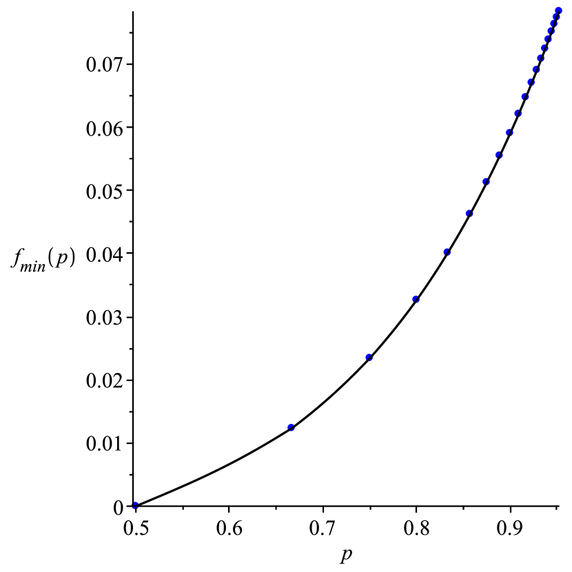
(a)

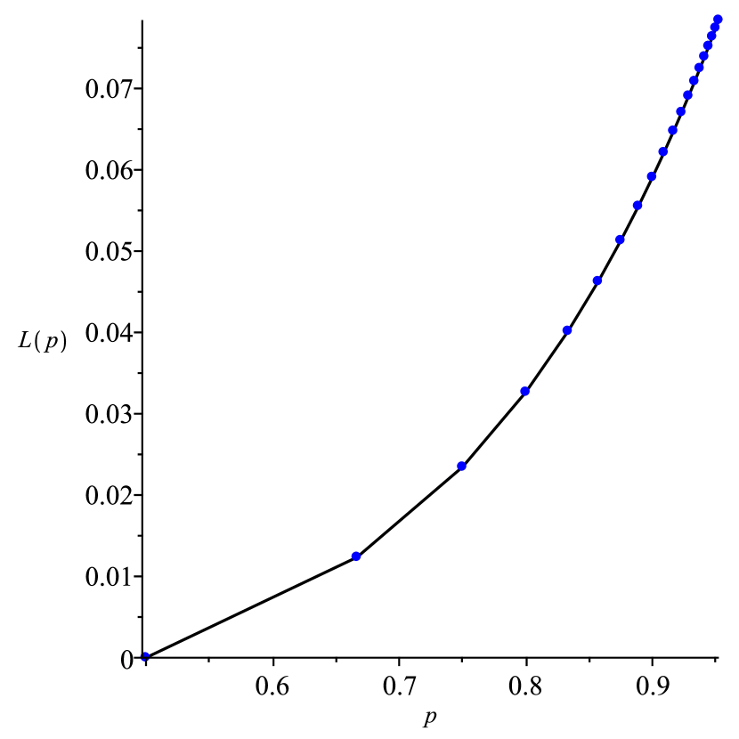
(b)

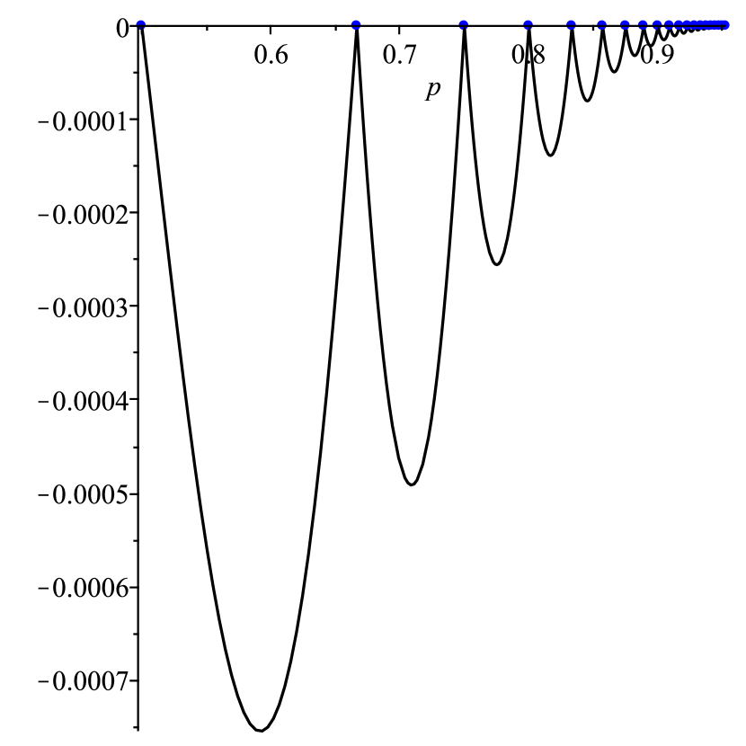
(c)

Figure 2: (2(a)) A graph of $f_{\min}(p)$ based on numerical calculations. Blue points correspond to the Turán densities (i.e. $p=1-1/k$). (2(b)) Secant lines between Turán densities. (2(c)) A graph of $f_{\min}(p)-L(p)$.

We now address what graphs are suitable for $G[Y]$, i.e. what graphs satisfy (i) and (ii). Note first that some such choice of $G[Y]$ exists, for example it can be a random bipartite graph with two parts of size $\frac{1}{2}yn$ and edge probability $2\rho$. Now we claim that $G[Y]$ satisfies (i) if and only if $G[Y]$ is almost $yn\rho$-regular, or more formally, all but $o(n)$ vertices in $G[Y]$ have degree $(1+o(1))yn\rho$. Indeed, if $G[Y]$ is almost $yn\rho$-regular then it is easy to verify the edge and path counts in (i). Conversely, suppose (i) holds, and let the random variable $Z$ represent the degree of a random vertex in $G[Y]$. Then we have $\mathbb{E}[Z]=(1+o(1))yn\rho$ and since $\sum_{v\in Y}\binom{deg(v)}{2}$ is the number of paths of length 2 we can calculate

$$\mathbb{E}[Z^{2}]= \frac{1}{yn}\sum_{v\in V(Y)}deg(v)^{2}=\frac{1}{yn}\cdot 2(1+o(1))\frac{1}{2}y^{3}n^{3}\rho^{2}=(1+o(1))y^{2}n^{2}\rho^{2}=(1+o(1))\mathbb{E}[Z]^{2}$$

so $Z$ is concentrated by Chebyshev’s inequality (see, e.g., Lemma 20.3 in [7]). In other words, $G[Y]$ is almost $yn\rho$-regular.

We believe that we have described all almost optimal graphs. Specifically, we believe that any graph with edge density $p$ and $C_{5}$-density $d_{C_{5}}(p)+o(1)$ can be transformed by adding or deleting at most $o(n^{2})$ edges into a graph with a vertex partition $X_{1},\ldots,X_{k-1},Y$ where $|X_{i}|=xn,|Y|=yn$, all $X_{i}$ are independent, all $X_{i}$ and $Y$ are complete to each other, and $G[Y]$ is $yn\rho$-regular where $x,y,\rho$ are a solution to the optimization problem (P).

Appendix A Appendix

$F$ $c_{F}^{OPT}$ 0 0 0 0 0 0 0 0 0 0 0 0 0 0 0 0 0 0 0 0 0 0 0 0 0 0 1 1 1 2 2 4 6 12 $p(K_{2},F)$ 0 1 2 3 4 3 2 3 4 3 4 5 4 5 4 5 5 6 6 7 6 4 5 6 7 6 5 6 7 7 8 8 9 10 $\llbracket X_{1}\times X_{1}\rrbracket_{1}$ 30 12 4 0 0 0 4 2 0 0 0 0 2 0 0 0 0 0 0 0 0 0 0 0 0 0 0 0 0 0 0 0 0 0 $\llbracket X_{1}\times X_{2}\rrbracket_{1}$ 0 3 4 3 0 6 0 1 2 0 0 0 0 1 0 0 0 0 0 0 0 0 0 0 0 0 0 0 0 0 0 0 0 0 $\llbracket X_{1}\times X_{3}\rrbracket_{1}$ 0 6 4 3 0 0 8 2 0 6 2 0 0 0 2 0 1 0 0 0 0 0 0 0 0 0 0 0 0 0 0 0 0 0 $\llbracket X_{1}\times X_{4}\rrbracket_{1}$ 0 0 2 6 12 0 0 2 2 0 3 4 0 0 0 2 0 1 0 0 0 0 0 0 0 0 0 0 0 0 0 0 0 0 $\llbracket X_{1}\times X_{5}\rrbracket_{1}$ 0 0 1 0 0 0 0 2 0 0 1 0 4 0 1 0 2 0 3 0 0 0 0 0 0 0 0 0 0 0 0 0 0 0 $\llbracket X_{1}\times X_{6}\rrbracket_{1}$ 0 0 0 0 0 3 0 0 2 0 0 2 0 2 0 1 0 2 0 3 0 0 0 0 0 0 0 0 0 0 0 0 0 0 $\llbracket X_{2}\times X_{2}\rrbracket_{1}$ 0 0 0 0 0 0 2 2 2 0 0 0 4 4 0 0 0 0 0 0 6 0 0 0 0 0 0 0 0 0 0 0 0 0 $\llbracket X_{2}\times X_{3}\rrbracket_{1}$ 0 0 0 0 0 0 4 2 1 4 2 0 0 0 2 2 0 0 0 0 0 6 2 1 0 0 0 0 0 0 0 0 0 0 $\llbracket X_{2}\times X_{4}\rrbracket_{1}$ 0 0 0 0 0 0 0 0 0 2 2 2 0 0 2 2 2 2 0 0 0 0 1 2 3 0 0 0 0 0 0 0 0 0 $\llbracket X_{2}\times X_{5}\rrbracket_{1}$ 0 0 0 0 0 0 0 0 0 1 0 0 0 0 2 0 1 0 0 0 0 0 1 0 0 0 5 2 0 1 0 0 0 0 $\llbracket X_{2}\times X_{6}\rrbracket_{1}$ 0 0 0 0 0 0 0 0 0 0 0 0 0 0 0 0 0 0 0 0 0 3 2 1 0 4 0 1 2 0 1 0 0 0 $\llbracket X_{3}\times X_{3}\rrbracket_{1}$ 0 0 4 0 0 12 0 4 4 4 0 0 0 0 6 2 0 0 0 0 0 12 4 0 0 0 10 2 0 0 0 0 0 0 $\llbracket X_{3}\times X_{4}\rrbracket_{1}$ 0 0 0 0 0 0 0 2 2 0 2 4 8 4 2 0 4 2 0 0 0 0 4 2 0 8 0 2 2 0 0 0 0 0 $\llbracket X_{3}\times X_{5}\rrbracket_{1}$ 0 0 0 3 0 0 0 0 2 0 2 0 0 2 0 2 1 0 0 0 0 0 2 2 0 0 0 2 0 2 0 0 0 0 $\llbracket X_{3}\times X_{6}\rrbracket_{1}$ 0 0 0 0 0 0 0 0 1 0 0 0 0 4 0 2 0 2 0 0 12 0 0 3 6 0 0 0 2 0 2 0 0 0 $\llbracket X_{4}\times X_{4}\rrbracket_{1}$ 0 0 0 0 0 0 0 0 0 0 0 0 0 0 2 2 4 4 12 12 0 0 0 0 0 0 10 6 4 4 4 0 0 0 $\llbracket X_{4}\times X_{5}\rrbracket_{1}$ 0 0 0 0 0 0 0 0 0 0 1 0 0 0 0 2 2 1 6 0 0 0 0 2 0 0 0 2 2 4 0 4 0 0 $\llbracket X_{4}\times X_{6}\rrbracket_{1}$ 0 0 0 0 0 0 0 0 0 0 0 0 0 0 0 0 0 0 0 0 0 0 1 2 3 0 0 2 2 6 4 8 6 0 $\llbracket X_{5}\times X_{5}\rrbracket_{1}$ 0 0 0 0 6 0 0 0 0 0 0 4 0 0 0 0 0 2 0 0 0 0 0 0 0 4 0 0 2 0 0 2 0 0 $\llbracket X_{5}\times X_{6}\rrbracket_{1}$ 0 0 0 0 0 0 0 0 0 0 0 1 0 0 0 0 0 2 0 6 0 0 0 0 3 0 0 0 1 0 4 0 3 0 $\llbracket X_{6}\times X_{6}\rrbracket_{1}$ 0 0 0 0 0 0 0 0 0 0 0 0 0 0 0 0 0 0 0 0 0 0 0 0 0 2 0 0 2 0 4 4 12 30

Table 1: All entries corresponding to $p(K_{2},F)$ are multiplied by 10 and all entries corresponding to $\llbracket X_{i}\times X_{j}\rrbracket_{1}$ are multiplied by 30.

Appendix B Appendix

This Maple code computes $c_{F}$ coefficients. Matrices $A$, $B$ and $M$ are defined in Subsection 2.2.2. $X$ is a matrix of size $21\times 34$ and it is defined in Appendix A (rows correspond to $\llbracket X_{i}\times X_{j}\rrbracket_{1}$). Vectors cFOPT, pF, cFM and cF (each of size 34) correspond to $\ c_{F}^{OPT},p(K_{2},F),c_{F}^{M}$ and $c_{F}$, respectively. Constant $a$ corresponds to $\alpha$.

[] restart: with(LinearAlgebra): A := Matrix([[32*k^2-96*k+96, 0, 4*k^2-16*k], [0, 10*k^4-30*k^3-8*k^2+96*k-96, -10*k^4+35*k^3-4*k^2-80*k+96], [4*k^2-16*k, -10*k^4+35*k^3-4*k^2-80*k+96, 10*k^4-40*k^3+24*k^2+64*k-96]]): B := Matrix([[k-1, 1, k-2, 0, k-3, -1], [0, 2, k-2, 0, 2*k-4, -2], [0, 0, k-1, -1, 2*k-2, -2]]): M:= (3/(2*k^4))*Matrix(Multiply(Transpose(B), Multiply(A, B))): X:=(1/30)*Matrix([[30,12,4,0,0,0,4,2,0,0,0,0,2,0,0,0,0,0,0,0,0,0,0,0,0,0,0,0,0,0,0,0,0,0], [0,3,4,3,0,6,0,1,2,0,0,0,0,1,0,0,0,0,0,0,0,0,0,0,0,0,0,0,0,0,0,0,0,0], [0,6,4,3,0,0,8,2,0,6,2,0,0,0,2,0,1,0,0,0,0,0,0,0,0,0,0,0,0,0,0,0,0,0], [0,0,2,6,12,0,0,2,2,0,3,4,0,0,0,2,0,1,0,0,0,0,0,0,0,0,0,0,0,0,0,0,0,0], [0,0,1,0,0,0,0,2,0,0,1,0,4,0,1,0,2,0,3,0,0,0,0,0,0,0,0,0,0,0,0,0,0,0], [0,0,0,0,0,3,0,0,2,0,0,2,0,2,0,1,0,2,0,3,0,0,0,0,0,0,0,0,0,0,0,0,0,0], [0,0,0,0,0,0,2,2,2,0,0,0,4,4,0,0,0,0,0,0,6,0,0,0,0,0,0,0,0,0,0,0,0,0], [0,0,0,0,0,0,4,2,1,4,2,0,0,0,2,2,0,0,0,0,0,6,2,1,0,0,0,0,0,0,0,0,0,0], [0,0,0,0,0,0,0,0,0,2,2,2,0,0,2,2,2,2,0,0,0,0,1,2,3,0,0,0,0,0,0,0,0,0], [0,0,0,0,0,0,0,0,0,1,0,0,0,0,2,0,1,0,0,0,0,0,1,0,0,0,5,2,0,1,0,0,0,0], [0,0,0,0,0,0,0,0,0,0,0,0,0,0,0,0,0,0,0,0,0,3,2,1,0,4,0,1,2,0,1,0,0,0], [0,0,4,0,0,12,0,4,4,4,0,0,0,0,6,2,0,0,0,0,0,12,4,0,0,0,10,2,0,0,0,0,0,0], [0,0,0,0,0,0,0,2,2,0,2,4,8,4,2,0,4,2,0,0,0,0,4,2,0,8,0,2,2,0,0,0,0,0], [0,0,0,3,0,0,0,0,2,0,2,0,0,2,0,2,1,0,0,0,0,0,2,2,0,0,0,2,0,2,0,0,0,0], [0,0,0,0,0,0,0,0,1,0,0,0,0,4,0,2,0,2,0,0,12,0,0,3,6,0,0,0,2,0,2,0,0,0], [0,0,0,0,0,0,0,0,0,0,0,0,0,0,2,2,4,4,12,12,0,0,0,0,0,0,10,6,4,4,4,0,0,0], [0,0,0,0,0,0,0,0,0,0,1,0,0,0,0,2,2,1,6,0,0,0,0,2,0,0,0,2,2,4,0,4,0,0], [0,0,0,0,0,0,0,0,0,0,0,0,0,0,0,0,0,0,0,0,0,0,1,2,3,0,0,2,2,6,4,8,6,0], [0,0,0,0,6,0,0,0,0,0,0,4,0,0,0,0,0,2,0,0,0,0,0,0,0,4,0,0,2,0,0,2,0,0], [0,0,0,0,0,0,0,0,0,0,0,1,0,0,0,0,0,2,0,6,0,0,0,0,3,0,0,0,1,0,4,0,3,0], [0,0,0,0,0,0,0,0,0,0,0,0,0,0,0,0,0,0,0,0,0,0,0,0,0,2,0,0,2,0,4,4,12,30]]): cFM := Vector(34): k_ind := 0: printlevel := 2: for i to 6 do for j from i to 6 do k_ind := k_ind+1; if i = j then cFM := cFM+M(i, j)*Transpose(Row(X, k_ind)); else cFM := cFM+2*M(i, j)*Transpose(Row(X,k_ind)); end if; end do; end do: cFOPT := Vector([0,0,0,0,0,0,0,0,0,0,0,0,0,0,0,0,0,0,0,0,0,0,0,0,0,0,1,1,1,2,2,4,6,12]): pF := (1/10)*Vector([0,1,2,3,4,3,2,3,4,3,4,5,4,5,4,5,5,6,6,7,6,4,5,6,7,6,5,6,7,7,8,8,9,10]): a := (1/(k^3))*(60*k^3 - 240*k^2 + 360*k - 192): cF := Vector(34): for i to 34 do cF(i) := cFOPT(i)-a*pF(i)-cFM(i)+(k-1)*a/k end do: for i to 34 do printf(”5*k^4*cF(end do: kernel := NullSpace(B): kernelMatrix := Matrix(convert(kernel, list)): ReducedRowEchelonForm(Transpose(kernelMatrix))

References

[1]
N. Alon, E. Fischer, M. Krivelevich, and M. Szegedy, Efficient testing of
large graphs, Combinatorica 20 (2000), no. 4, 451–476.
[2]
J. Balogh, P. Hu, B. Lidický, and F. Pfender, Maximum density of
induced 5-cycle is achieved by an iterated blow-up of 5-cycle, European J.
Combin. 52 (2016), no. part A, 47–58.
[3]
B. Borchers, CSDP, a C library for semidefinite programming,
Optimization Methods and Software 11 (1999), no. 1-4, 613–623.
[4]
D. Conlon and J. Fox, Graph removal lemmas, Surveys in combinatorics
2013, London Math. Soc. Lecture Note Ser., vol. 409, Cambridge Univ. Press,
Cambridge, 2013, pp. 1–49.
[5]
P. Erdős, On some problems in graph theory, combinatorial analysis
and combinatorial number theory, Graph theory and combinatorics
(Cambridge, 1983), Academic Press, London, 1984, pp. 1–17.
[6]
P. Erdős and A. H. Stone, On the structure of linear graphs, Bull.
Amer. Math. Soc. 52 (1946), 1087–1091.
[7]
A. Frieze and M. Karoński, Introduction to random graphs, Cambridge
University Press, Cambridge, 2016.
[8]
A. Grzesik, On the maximum number of five-cycles in a triangle-free
graph, J. Combin. Theory Ser. B 102 (2012), no. 5, 1061–1066.
[9]
H. Hatami, J. Hladký, D. Král’, S. Norine, and A. Razborov, On the
number of pentagons in triangle-free graphs, J. Combin. Theory Ser. A
120 (2013), no. 3, 722–732.
[10]
B. Lidický and F. Pfender, Pentagons in triangle-free graphs, European
J. Combin. 74 (2018), 85–89.
[11]
H. Liu, O. Pikhurko, M. Sharifzadeh, and K. Staden, Stability from
symmetrisation arguments, work in progress, 2019.
[12]
H. Liu, O. Pikhurko, and K. Staden, The exact minimum number of triangles
in graphs of given order and size, arXiv:1712.00633.
[13]
L. Lovász, Large networks and graph limits, Colloquium Publications,
Amer. Math. Soc., 2012.
[14]
L. Lovász and M. Simonovits, On the number of complete subgraphs of a
graph. II, Studies in pure mathematics, Birkhäuser, Basel, 1983,
pp. 459–495.
[15]
L. Lovász and B. Szegedy, Limits of dense graph sequences, J. Combin. Theory (B) 96 (2006), 933–957.
[16]
, Testing properties of graphs and functions, Israel J. Math.
178 (2010), 113–156.
[17]
W. Mantel, Problem 28, Winkundige Opgaven 10 (1907), 60–61.
[18]
J. W. Moon and L. Moser, On a problem of Turán, Magyar Tud. Akad.
Mat. Kutató Int. Közl. 7 (1962), 283–286.
[19]
V. Nikiforov, The number of cliques in graphs of given order and size,
Trans. Amer. Math. Soc. 363 (2011), no. 3, 1599–1618.
[20]
E. A. Nordhaus and B. M. Stewart, Triangles in an ordinary graph, Canad.
J. Math. 15 (1963), 33–41.
[21]
O. Pikhurko, An analytic approach to stability, Discrete Math.
310 (2010), 2951–2964.
[22]
O. Pikhurko and A. Razborov, Asymptotic structure of graphs with the
minimum number of triangles, Combin. Probab. Comput. 26 (2017),
no. 1, 138–160.
[23]
O. Pikhurko, J. Sliacan, and K. Tyros, Strong forms of stability from
flag algebra calculations, J. Combin. Theory (B) 135 (2019),
129–178.
[24]
N. Pippenger and M. C. Golumbic, The inducibility of graphs, J.
Combinatorial Theory Ser. B 19 (1975), no. 3, 189–203.
[25]
A. Razborov, Flag algebras, J. Symbolic Logic 72 (2007), no. 4,
1239–1282.
[26]
, On the minimal density of triangles in graphs, Combin. Probab.
Comput. 17 (2008), no. 4, 603–618.
[27]
Ch. Reiher, The clique density theorem, Ann. of Math. (2) 184
(2016), no. 3, 683–707.
[28]
A.F. Sidorenko, Inequalities for functionals generated by bipartite
graphs, Diskret. Mat. 3 (1991), no. 3, 50–65.
[29]
P. Turán, Eine Extremalaufgabe aus der Graphentheorie, Mat. Fiz.
Lapok 48 (1941), 436–452.